The VLA/ALMA Nascent Disk and Multiplicity (VANDAM) Survey of Orion Protostars. A Statistical Characterization of Class 0 and I Protostellar Disks

Abstract

We have conducted a survey of 328 protostars in the Orion molecular clouds with ALMA at 0.87 mm at a resolution of $\sim$0$\farcs$1 (40 au), including observations with the VLA at 9 mm toward 148 protostars at a resolution of $\sim$0$\farcs$08 (32 au). This is the largest multi-wavelength survey of protostars at this resolution by an order of magnitude. We use the dust continuum emission at 0.87 mm and 9 mm to measure the dust disk radii and masses toward the Class 0, Class I, and Flat Spectrum protostars, characterizing the evolution of these disk properties in the protostellar phase. The mean dust disk radii for the Class 0, Class I, and Flat Spectrum protostars are 44.9${}^{+5.8}_{-3.4}$, 37.0${}^{+4.9}_{-3.0}$, and 28.5${}^{+3.7}_{-2.3}$ au, respectively, and the mean protostellar dust disk masses are 25.9${}^{+7.7}_{-4.0}$, 14.9${}^{+3.8}_{-2.2}$, 11.6${}^{+3.5}_{-1.9}$ M_⊕, respectively. The decrease in dust disk masses is expected from disk evolution and accretion, but the decrease in disk radii may point to the initial conditions of star formation not leading to the systematic growth of disk radii or that radial drift is keeping the dust disk sizes small. At least 146 protostellar disks (35% out of 379 detected 0.87 mm continuum sources plus 42 non-detections) have disk radii greater than 50 au in our sample. These properties are not found to vary significantly between different regions within Orion. The protostellar dust disk mass distributions are systematically larger than that of Class II disks by a factor of $>$4, providing evidence that the cores of giant planets may need to at least begin their formation during the protostellar phase.

1 Introduction

The formation of stars and planets is initiated by the gravitational collapse of dense clouds of gas and dust. In order for gravitational collapse to proceed, other sources of support (e.g., thermal pressure, magnetic fields, turbulence; McKee & Ostriker, 2007) must either be reduced or not significant at the onset of collapse. As the protostar is forming within a collapsing envelope of gas and dust, a rotationally-supported disk is expected to form around the protostar via conservation of angular momentum. Once a disk has formed, the majority of accretion onto the star will happen through the disk, and the disk material is expected to provide the raw material for planet formation.

The angular momentum that drives disk formation may originate from rotation of the core ($\sim$0.05 pc in diameter), but organized rotation of cores is found less frequently as cores are observed with higher angular resolution and sensitivity (e.g., Tobin et al., 2011, 2012, 2018, Chen et al. 2019). Thus, the angular momentum may not derive from organized core rotation. The origin of the net angular momentum is not specifically important, but within larger-scale molecular clouds (1 - 10 pc), the angular momentum within cores that leads to the formation of disks likely derives from the residual core-scale turbulent motion of the gas or gravitational torques between overdensities in the molecular cloud (Burkert & Bodenheimer, 2000; Offner et al., 2016; Kuznetsova et al., 2019). However, in order for conservation of angular momentum to lead to the formation of disks around protostars (e.g., Terebey et al., 1984), magnetic fields must not be strong enough or not coupled strongly enough to the gas to prevent the spin-up of infalling material as it conserves angular momentum during collapse (Allen et al., 2003; Mellon & Li, 2008; Padovani et al., 2013). On the other hand, non-ideal magneto-hydrodynamic effects (MHD) can also dissipate the magnetic flux and enable the formation of disks to proceed (e.g., Dapp & Basu, 2010; Li et al., 2014; Masson et al., 2016; Hennebelle et al., 2016), as can turbulence and/or magnetic fields misaligned with the core rotation axis (Seifried et al., 2012; Joos et al., 2012).

The youngest observationally recognized protostars are those in the Class 0 phase, in which a dense infalling envelope of gas and dust surrounds the protostar (André et al., 1993). The Class I phase follows, where the protostar is less deeply embedded, but still surrounded by an infalling envelope. The transition between Class 0 and Class I is not exact, but a bolometric temperature (T_bol) of 70 K or L_bol/L_submm $<$ 0.005 have been adopted as the divisions between the classes. T_bol is a typical diagnostic to characterize the evolutionary state of a young star (Ladd et al., 1993; Dunham et al., 2014). The envelope is expected to be largely dissipated by the end of the Class I phase, leaving a disk surrounding a pre-main sequence star, also known as Class II YSOs, which have T_bol $>$ 650 K (e.g., Dunham et al., 2014). Furthermore, a possible transition phase prior to becoming a Class II YSO, known as Flat Spectrum sources, also exists. These protostars are characterized by a flat spectral energy distribution (SED) in $\lambda$F_λ from $\sim$2 µm to 24 µm. The nature of Flat Spectrum sources with respect to Class I sources is still unclear. Some Flat Spectrum sources are suggested to be Class II based on their lack of dense molecular gas (van Kempen et al., 2009; Heiderman & Evans, 2015), but SED modeling of the Flat Spectrum sources in Orion found that they were best fit by models with an envelope in the majority of systems (Furlan et al., 2016). The length of the protostellar phase (Class 0, I, and Flat Spectrum) combined has been estimated to be $\sim$500 kyr and the Class 0 phase itself is estimated to last $\sim$160 kyr (Dunham et al., 2014). However, Kristensen & Dunham (2018) used a different set of assumptions to derive half-lives of the protostellar phase in which the Class 0, Class I, and Flat Spectrum phases have half-lives of 74 kyr, 88 kyr, and 87 kyr, respectively, 222 kyr in total.

Disks are observed nearly ubiquitously toward the youngest stellar populations that are dominated by Class II YSOs, and the frequency of disks within a population declines for older associations of YSOs (Hernández et al., 2008). This high occurrence rate of disks in later stages is an indication that disk formation is a universal process in star formation. These disks around pre-main-sequence stars have been commonly referred to as protoplanetary disks or Class II disks, and to draw distinction between disks around YSOs in the protostellar phase (Class 0, I, and Flat Spectrum), we will generically refer to the latter as protostellar disks.

The observed properties of disks throughout the protostellar phase will both inform us of the conditions of their formation as well as the initial conditions for disk evolution. The properties of Class 0 disks have been sought after with (sub)millimeter and centimeter-wave interferometry, and each increase in the capability of interferometers at these wavelengths has led to new constraints on the properties of Class 0 disks from their dust emission. Brown et al. (2000) used a single baseline interferometer formed by the James Clerk Maxwell Telescope (JCMT) and the Caltech Submillimeter Observatory (CSO) to characterize the disk radii toward a number of Class 0 protostars. Looney et al. (2000) used the Berkeley Illinois Maryland Array (BIMA) to resolve a number of Class 0, Class I, and Class II protostars, measuring disk radii, masses, and multiple systems. Harvey et al. (2003) used the Plateau de Bure Interferometer (PdBI) to characterize the unresolved disk toward B335, finding a dust disk with a radius less than 100 au and a dust mass of $\sim$4$\times$10^-5 M_☉. However, the sensitivity and resolution of these earlier instruments was not sufficient to characterize the disks with extremely high fidelity, nor were samples large enough to be statistically meaningful.

Larger samples of disks and higher-fidelity imaging with upgraded interferometers began with the Submillimeter Array (SMA), using unresolved observations to infer the masses of protostellar disks from the Class 0 to Class I phase (Jørgensen et al., 2009). Maury et al. (2010) observed 5 Class 0 protostars with the PdBI, which only had sufficient resolution to detect dust disks with radii larger than $\sim$150 au and none were positively identified. Chiang et al. (2012) used multi-configuration observations with the Combined Array for Millimeter-wave Astronomy (CARMA) toward the Class 0 protostar L1157-mm to identify a candidate unresolved disk with a radius smaller than $\sim$100 au. Also, Enoch et al. (2011) examined a sample of 9 candidate protostellar disks in Serpens, including a possible disk toward the Class 0 protostar Serpens FIRS1 (Enoch et al., 2009). Despite the improved sensitivity of these instruments, most studies were limited to characterizing disks via dust continuum emission with a best resolution of $\sim$0$\farcs$3 ($\sim$120 au). This means that these observations only primarily probed the dust disks and not the gas disks.

Molecular line observations were possible toward some of the most nearby protostellar disks with the previous generation of instruments. Tobin et al. (2012) were able to use CARMA to positively resolve the disk toward the Class 0 protostar L1527 IRS in the dust continuum and identify likely Keplerian rotation from ¹³CO emission, and Murillo & Lai (2013) detected possible evidence of disk rotation toward VLA 1623 with the SMA, which is now recognized to be a triple system with a circum-multiple disk (Harris et al., 2018; Sadavoy et al., 2018). At the same time, observations of disks toward Class I protostars had also yielded some detections of resolved disks and Keplerian rotation (Wolf et al., 2008; Takakuwa et al., 2012; Launhardt et al., 2009; Harsono et al., 2014; Harris et al., 2018; Alves et al., 2018).

The advent of the Atacama Large Millimeter/submillimeter Array (ALMA) came on the heels of these pioneering studies with more than an order of magnitude greater sensitivity and angular resolution. ALMA is leading a revolution in the characterization of individual protostellar disks, confirming and extending earlier results such as the Class 0 rotationally-supported disk around L1527 IRS (Ohashi et al., 2014; Sakai et al., 2014; Aso et al., 2017). Furthermore, a number of new Class 0 disks have been identified and confirmed to be rotationally-supported (Murillo et al., 2013; Lindberg et al., 2014; Codella et al., 2014; Yen et al., 2017; Alves et al., 2018), and some very small Class 0 disks have also been identified (Yen et al., 2015; Hsieh et al., 2019). At the same time, the characterization of Class I disks has been progressing (Yen et al., 2014; Aso et al., 2015; Sakai et al., 2016). Finally, a number of circum-binary and circum-multiple disks have been identified in both the Class 0 and Class I phase (Tobin et al., 2016a; Takakuwa et al., 2014; Harris et al., 2018; Sadavoy et al., 2018).

A trend that has emerged from the aforementioned studies of Class 0 disks is that, when a disk-like morphology is resolved in the dust continuum toward Class 0 and I protostars, this structure is a rotationally supported disk. Thus, if a disk-like continuum feature is well-resolved, then it is likely that this feature reflects a rotationally-supported disk. This has enabled larger surveys that focus primarily on continuum sensitivity to characterize larger samples of Class 0 and I disks. Segura-Cox et al. (2016, 2018) used the data from the NSF’s Karl G. Jansky Very Large Array (VLA) taken as part of the VLA Nascent Disk and Multiplicity (VANDAM) Survey, to identify a total of 18 Class 0 disk candidates (out of 37 Class 0 protostars and 8 Class 0/I protostars observed), many with radii less than 30 au, greatly increasing the range of scales at which Class 0 disk candidates have been resolved. Finally, Maury et al. (2018) used the IRAM-PdBI to conduct a survey of 16 Class 0 protostars as part of the Continuum And Lines in Young Protostellar Objects (CALYPSO) Survey in both lines and continuum. The continuum observations found that 4 out of 16 protostars have evidence for disks with radii $>$ 60 au. While these new continuum surveys are important for increasing the statistics, the CALYPSO survey was limited in both sensitivity and angular resolution (0$\farcs$3), while the VANDAM survey had excellent angular resolution ($\sim$0$\farcs$07), but limited surface brightness and dust mass sensitivity due to the 9 mm wavelength of the observations.

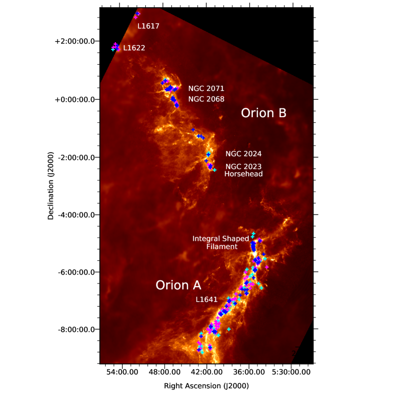
Figure 1: Overview of the Orion region and protostellar targets for the ALMA and VLA surveys (crosses). The image is the Herschel and Planck column density map from Lombardi et al. (2014) displayed on a square-root color scale. Major sub-regions within the clouds are highlighted with the sub-region labels located adjacent to their positions. The blue crosses are Class 0 protostars, magenta crosses are Class I protostars, and cyan crosses are Flat Spectrum protostars.

A principal limitation of protostellar disk studies has been the sample size. Protostars are inherently rarer than the more-evolved pre-main sequence stars with disks, making their populations in the nearby star-forming regions small. For this reason, Orion is an essential region to study in order to obtain a representative characterization of protostellar disk characteristics. Orion is the nearest region forming massive stars and richest region of low-mass star formation within 500 pc. Orion is also the best analogue for examining star and planet formation in an environment that is likely representative of most star formation in our Galaxy. Studies of Orion with the Spitzer Space Telescope and Herschel Space Observatory have identified at least 428 protostar candidates in Orion (Class 0 through Flat Spectrum), in addition to 2991 more-evolved dusty young stars (Class II and III; Megeath et al., 2012; Furlan et al., 2016). Therefore, while the more nearby regions like Taurus and Perseus enable protostellar disks to be resolved in greater detail, Orion provides a much larger sample of protostars than the nearby star-forming regions. Orion contains nearly as many protostars as the rest of the Gould Belt, which encompasses all the other star-forming regions within 500 pc (Dunham et al., 2015). Orion is composed of two main molecular clouds that are known as the Orion A and Orion B molecular clouds (see Figure 1). Orion A contains the most active region of star formation, harboring the Integral-Shaped Filament, the Trapezium, and Orion BN-KL, while Orion B also has massive star formation, as well as the second (NGC 2024) and third (NGC 2068/2071) most massive clusters in Orion (Megeath et al., 2016). The entire Orion complex spans $\sim$83 pc projected on the plane of the sky, but the protostars are preferentially located in regions of high gas column density. Both Orion A and Orion B contain clustered and isolated protostars, and the majority of protostars are not in close proximity to the Orion Nebula. Despite being a single region, there is significant distance variation across the plane of the sky. The Orion Nebula Cluster, the southern end of Orion A, and Orion B have typical distances of 389 pc, 443 pc, and 407 pc, respectively (Kounkel et al., 2017, 2018).

The high angular resolution and sensitivity to continuum emission makes ALMA uniquely suited to characterize the properties of protostellar disks for large samples such as Orion. However, even at submillimeter wavelengths the protostellar disks can be optically thick; therefore, VLA observations at 9 mm are crucial to examine the inner disks. This has motivated us to conduct the VLA/ALMA Nascent Disk and Multiplicity (VANDAM) survey toward all well-characterized protostars in the Orion A and B molecular clouds using ALMA and with VLA observations toward all the Class 0 and the youngest Class I protostars. We have used the ALMA and VLA data to characterize the dust disk masses and radii toward a sample of 328 protostars to better understand the structure of disks throughout the entire protostellar phase. This is the largest protostellar disk survey to date by an order of magnitude. The ALMA and VLA observations are described in Section 2. The results from continuum observations toward all sources are presented in Section 3. We discuss our results in Section 4 and present our conclusions in Section 5.

2 Observations and Data Reduction

2.1 The Sample

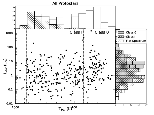
Figure 2: Bolometric luminosity (L_bol) versus bolometric temperature (T_bol) for the sample of 328 protostars surveyed by ALMA and the VLA with accompanying histograms. The histogram along the x-axis shows the full number in each bin, and the hatched region shows the number of Flat Spectrum sources, given that they overlap in this parameter space. The histogram along the y-axis shows the distribution bolometric luminosities for each protostellar class in the survey. The distributions are similar, but as shown in Fischer et al. (2017) the Class 0 protostars have slightly higher luminosities on the whole than the Class I and Flat Spectrum protostars.

The sample of protostars is drawn from the Herschel Orion Protostar Survey (HOPS; Fischer et al., 2010; Stutz et al., 2013; Furlan et al., 2016). We selected all Class 0, Class I, and Flat Spectrum protostars from the survey that had reliable measurements of bolometric temperature (T_bol), bolometric luminosity (L_bol), 70 µm detections, and were not flagged as extragalactic contaminants. From that sample of 409 HOPS protostars, we selected 320 HOPS protostars for observations with ALMA using the aforementioned criteria. We also included a few sources that were not part of the HOPS sample but are bonafide protostars in Orion B (HH270VLA1, HH270mms1, HH270mms2, HH212mms, HH111mms; Reipurth et al., 1999; Choi & Tang, 2006; Wiseman et al., 2001; Lee et al., 2017), and 3 unclassified protostellar candidates from Stutz et al. (2013) (S13-021010, S13-006006, S13-038002). This makes the total number of protostellar systems observed 328, of which 94 are Class 0 protostars, 128 are Class I protostars, 103 are Flat spectrum sources, and 3 were unclassified but expected to be Class 0 or I. The luminosity range of the sample is 0.1 L_☉ to $\sim$1400 L_☉. An overview image of the Orion region with the targeted protostars overlaid is shown in Figure 1, and we show a plot of L_bol vs. T_bol for the sample in Figure 2.

There is a distance variation on the order of $\pm$40 pc across the Orion A and B molecular clouds (Kounkel et al., 2017, 2018). To mitigate its impact on our analysis, we take advantage of the availability of Gaia data for a large sample of more evolved members within Orion, enabling us to estimate the distance toward each protostellar system. These distance estimates enable more precise calculations of the physical properties of the systems and comparison of the flux densities on a common scale. The method for estimating the distances is described in Appendix A; however, with respect to the typical distance of 400 pc to the region, the distances are all within $\sim$10% of this value.

2.2 ALMA 0.87 mm Observations

ALMA is located in northern Chile on the Chajnantor plateau at an elevation of $\sim$5000 m. The protostars in Orion selected for observations with ALMA at 0.87 mm were divided into three scheduling blocks. One scheduling block contained the selected protostars in the Orion B molecular cloud and two other scheduling blocks contained the selected protostars in the Orion A molecular cloud. Each scheduling block was successfully executed three times for nine executions in total. Six were executed in 2016 September, and three were executed in 2017 July. The date of each observation, number of antennas, precipitable water vapor, and maximum baseline are given in Table 1; the combined datasets sample baseline lengths from $\sim$15 m to $\sim$3700 m. We list the targeted protostars in Table 2; the total time on each source was $\sim$0.9 minutes.

The correlator was configured to provide high continuum sensitivity. We used two basebands set to low spectral resolution continuum mode, 1.875 GHz bandwidth divided into 128, 31.25 MHz channels, centered at 333 GHz and 344 GHz. We also observed ¹²CO ($J=3\rightarrow 2$) at 345.79599 GHz and ¹³CO ($J=3\rightarrow 2$) at 330.58797 GHz. The baseband centered on ¹²CO ($J=3\rightarrow 2$) had a total bandwidth of 937.5 MHz and 0.489 km s^-1 channels, and the baseband centered on ¹³CO ($J=3\rightarrow 2$) had a bandwidth of 234.375 MHz with 0.128 km s^-1 channels. The line-free regions of the ¹²CO and ¹³CO basebands were used for additional continuum bandwidth, resulting in an aggregate continuum bandwidth of $\sim$4.75 GHz.

The calibrators used for each execution are listed in Table 1. The data were manually reduced by the Dutch Allegro ARC Node using the Common Astronomy Software Application (CASA McMullin et al., 2007). The manual reduction was necessary to compensate for variability of the quasar J0510+1800 that was used for absolute flux calibration in some executions. The absolute flux calibration accuracy is expected to be $\sim$10%, and comparisons of the observed flux densities for the science targets during different executions are consistent with this level of accuracy. However, we only use statistical uncertainties for the flux density measurements and their derived quantities throughout the paper.

After the standard calibration, we performed up to three rounds of phase-only self-calibration on the continuum data to increase the S/N. The ability to self-calibrate depends on the S/N of the data, and we only attempted self calibration when the S/N of the emission peak was $>$10. For each successive round of self-calibration, we used solution intervals that spanned the entire scan length for the first round, as short as 12.08 s in the second round, and as short as 3.02 s in the third round, which was the length of a single integration. The solution interval was adjusted in the second and/or third round depending on the S/N of the source and the number of flagged solutions reported. We applied the self-calibration solutions using the CASA applycal task using applymode=calonly to avoid flagging data for which a self-calibration solution did not have high enough S/N to converge on a solution in a given round of self-calibration, but were otherwise good. Given the short total time on source, our observations were able to reach close to the thermal noise limit and were not strongly limited by dynamic range in most instances.

Following the continuum self-calibration, the phase solutions were then applied to the ¹²CO and ¹³CO spectral line data. The typical root-mean-squared (RMS) noise of the continuum, ¹²CO, and ¹³CO are 0.31 mJy beam^-1, 17.7 mJy beam^-1 (1 km s^-1 channels), and 33.3 mJy beam^-1 (0.5 km s^-1 channels), respectively. The spectral line observations were averaged by two and four channels for ¹²CO and ¹³CO, respectively, to reduce noise. The continuum and spectral line data cubes were imaged using the clean task of CASA 4.7.2 for all self-calibration and imaging.

The aggregate continuum image was reconstructed using Briggs weighting with a robust parameter of 0.5, yielding a synthesized beam of $\sim$0$\farcs$11 (44 au). We also made images with robust=2, 0, and -0.5, but we primarily use the robust=0.5 images in this paper, providing a compromise between sensitivity and angular resolution. For protostars that are not well-detected, we use the robust=2 images.

The continuum images are reconstructed only using uv-points at baselines $>$25 k$\lambda$ to mitigate striping resulting from large-scale emission that is not properly recovered. This data selection typically only removes a single baseline, and there is a gap between the shortest baseline and where the density of uv-points increases significantly. We used a different approach for the spectral line data because the ¹²CO and ¹³CO emission is typically much more extended than the continuum. We imaged the spectral line data using Natural weighting for baselines $>$50 k$\lambda$ to mitigate striping and with an outer taper of 500 k$\lambda$ applied to increase the sensitivity to extended structure; this yielded synthesized beams of $\sim$0$\farcs$25. However, we focus on the continuum for the remainder of this paper and do not discuss the spectral line data further.

2.3 VLA Observations

We conducted observations with the VLA in A-configuration between 2016 October 20 and 2017 January 07 in $\sim$100 individual observations; the observations are detailed in Table 3. We also conducted observations of the sources in C-configuration during February and March of 2016 with $\sim$1″ resolution, but these data were primarily used for A-configuration target selection and are not utilized in this paper except for a few upper limits. The targeted fields are detailed in Table 4.

The observations used the Ka-band receivers and the correlator was used in the wide bandwidth mode (3-bit samplers) with one 4 GHz baseband centered at 36.9 GHz (8.1 mm) and the other baseband was centered at 29 GHz (1.05 cm). Most observations were conducted in $\sim$2.5 hour scheduling blocks toward a single source with $\sim$1 hour on-source. However, a few observations were conducted in 4 hour scheduling blocks, observing two sources, each for $\sim$ 1 hr. In all observations, the absolute flux calibrator was 3C48 (J0137+3309), the bandpass calibrator was 3C84 (J0319+4130), and the complex gain calibrator was either J0552+0313 or J0541-0541 for protostars associated with Orion B or Orion A, respectively. The observations were conducted in fast-switching mode ($\sim$2.6 minute cycle times) to reduce phase decoherence in the high frequency observations, and between 25 and 27 antennas were available during each observation. The antenna pointing corrections were updated prior to observing the flux calibrator, bandpass calibrator, before the first observation of the complex gain calibrator, and after one hour had elapsed since the last pointing update. The absolute calibration uncertainty of the VLA data is expected to be $\sim$10%, and, similar to the ALMA data, we only report the statistical uncertainties in this paper.

The data were reduced using the scripted version of the VLA pipeline in CASA 4.4.0. We note that some of our observations were obtained during the period where the tropospheric delay correction was being misapplied to all VLA data; all A-configuration data prior to 2016 November 14 were affected. This resulted in a phase offset that was larger for lower elevations and when the angular separation of the source to the calibrator was large. When this error was integrated over an entire scheduling block that included observations at elevation below 30°, the continuum images would be smeared in the direction of elevation. However, we did not have a large separation between source and calibrator in most cases and the data were not taken for long periods at below 30° elevation. For sources that were determined to be strongly affected by the delay error, we utilized CASA 4.5.2 to run the VLA pipeline which incorporated a fix for the delay error.

We performed phase-only self-calibration on HOPS-370, HOPS-384, and HOPS-361 because these fields had high enough S/N to be dynamic range limited ($>$100). To perform self calibration, we used two solution intervals of 230 s (first round) and 90 s (second round), which corresponded to one solution for every two scans and one solution for each scan, respectively.

The continuum data for all sources were imaged using the clean task in CASA 4.5.1 using Natural weighting and multi-frequency synthesis with nterms=2 across both basebands. The final images have an RMS noise of $\sim$7-8 $\mu$Jy beam^-1 and a synthesized beam of $\sim$0$\farcs$08 (32 au).

2.4 Data Analysis

We fit elliptical Gaussians to each detected source using the imfit task of CASA 4.7.2. This enables us to measure the flux density of each source, its size, and its orientation from the major and minor axes of the Gaussian fits. While Gaussian fitting has limitations, its advantage lies in its simplicity and ability to rapidly fit a large number of sources. The principal metrics that we aim to derive are the protostellar disk radii and masses. Other methods used to observationally estimate disk radii include the curve of growth method used on the Lupus survey (Ansdell et al., 2016) and fitting a ‘Nuker profile’ (Tripathi et al., 2017). However, these methods are less ideal for protostellar disks. The curve of growth method works best if the orientation of the disk can be determined from its observed aspect ratio, enabling its visibility data and images to be deprojected, and the ’Nuker profile’ requires an assumption of an intensity profile. These methods and assumptions are not always possible and/or reliable for protostellar disks, due in large part to the surrounding envelope. Thus, these other methods will not necessarily lead to better results for protostellar disks.

We note that the curve of growth methodology employed by Ansdell et al. (2016) defined the disk radius as the radial point which contains 90% of the total flux density. When compared with a Gaussian fit, this is approximately the 2$\sigma$ point of a Gaussian. If one considers exponentially tapered disks, with a surface density profile defined as $\Sigma$ $\propto$ (R/R_C)^-γ, following the discussion in Bate (2018) for $\gamma$ $<$ 2, R_C always encompasses 63.2% of the dust disk mass, close to the 1$\sigma$ value of a Gaussian (68%). R_C is the critical radius, where the surface density of the disk begins to be truncated with an exponential taper. If the disks have a power-law surface density profile (exponentially-tapered or not), their intensity profile will not necessarily be well-described by a Gaussian when resolved. In fact, a Gaussian can systematically underestimate the size of an object with a power-law surface density (and intensity) profile due to a power-law decaying more slowly than a Gaussian. However, despite these caveats, we adopt the 2$\sigma$ size of the deconvolved major axis as a proxy for disk radius. Its value represents a compromise between potentially overestimating the disk radii by using a radius defined by the 90% level of the total flux density (e.g., Ansdell et al., 2018) and underestimating the disk radius by using 1$\sigma$. To convert to a radius in au, we multiply the full-width at half-maximum (FWHM) (in arcsec) by 2.0/2.355 and multiply by the estimated distance (in pc) toward the protostar. This radius will contain $\sim$95% of the flux density within the fitted Gaussian. Assuming that the submillimeter/centimeter flux density traces mass, then the 2$\sigma$ radius may be somewhat larger than the expected $R_{C}$ for exponentially tapered disks, but the 2$\sigma$ radius can also systematically underestimate the full radius of the disks if they are not well-described by Gaussians.

The integrated flux density measured with the Gaussian fit is used to analytically estimate the mass of the protostellar disks in each detected system. We make the assumption that the disk is isothermal and optically thin, enabling us to use the equation

$$M_{dust}=\frac{D^{2}F_{\nu}}{\kappa_{\nu}B_{\nu}(T_{dust})},$$ (1)

where D is the estimated distance toward the protostar, $F_{\nu}$ is the observed flux density, $B_{\nu}$ is the Planck function, $T_{dust}$ is the dust temperature, and $\kappa_{\nu}$ is the dust opacity at the observed wavelength. If the dust emission is not optically thin, then the masses will be lower limits. We adopt $\kappa_{0.87mm}$ = 1.84 cm² g^-1 from Ossenkopf & Henning (1994), and at 9.1 mm we adopt a dust opacity of 0.13 cm² g^-1 by extrapolating from the Ossenkopf & Henning (1994) dust opacity at 1.3 mm (0.899 cm² g^-1) assuming a dust opacity spectral index of 1.

In the literature, T_dust is typically assumed to be 30 K for solar-luminosity protostars (Tobin et al., 2015a, 2016b; Tychoniec et al., 2018). Given the wide range of luminosities for the protostars in Orion (see Figure 2; Fischer et al., 2017), it is essential that we scale T_dust using the bolometric luminosity for each system in order to obtain more realistic dust mass measurements. We used a grid of radiative transfer models to calculate the appropriate average temperature to use for protostellar disks found in systems with particular luminosities and radii (Appendix B). We note, however, that the dust emission from the disks can be optically thick, resulting in underestimates of the dust disk masses.

Based on these models, we adopt an average dust temperature of

$$T_{dust}=T_{0}\left(\frac{L_{bol}}{1~{}L_{\odot}}\right)^{0.25}$$ (2)

where T₀ = 43 K, and we scale this using L_bol for each protostellar system. The average dust temperature of 43 K is reasonable for a $\sim$1 L_☉ protostar at a radius of $\sim$50 au (see Appendix B; Whitney et al., 2003; Tobin et al., 2013). While Tazzari et al. (2017) demonstrated that the dust temperature of Class II disks is typically independent of total luminosity, the dust temperature of disks embedded within envelopes are not independent of luminosity due to the surrounding envelope also illuminating the disk (see also Osorio et al. 2003 and Appendix B for further details). Other studies have similarly employed such corrections to the average dust temperatures to obtain more realistic mass measurements (e.g., Jørgensen et al., 2009; Andrews et al., 2013; Ward-Duong et al., 2018). Our 3$\sigma$ detection limit at 0.87 mm ($\sim$1 mJy beam^-1) corresponds to $\sim$1.1 $M_{\earth}$ for a 1 L_☉ protostar (T_dust = 43 K), and the 3$\sigma$ limit at 9 mm ($\sim$25 $\mu$Jy beam^-1) corresponds to 35 $M_{\earth}$.

3 Results

The ALMA and VLA continuum images reveal compact dusty structures on scales $\lesssim$2″ toward the sampled protostars in Orion. The observations have very limited sensitivity to structure larger than 2″ due to the data being taken in high-resolution configurations with few short baselines. The ALMA and VLA surveys detected the protostellar sources (i.e., dust emission from their disks and/or inner envelopes) in their targeted fields with a small percentage of non-detections, producing a large sample of sources observed at high angular resolution from submillimeter to centimeter wavelengths.

3.1 Detection Statistics

Out of 328 protostars targeted with ALMA, 94 are Class 0 protostars, 128 are Class I protostars, 103 are Flat Spectrum protostars, and 3 are unclassified but presumed protostars. The detection statistics are summarized in Table 5. We detected continuum emission associated with the protostars in 286 fields with at least S/N $>$ 3, corresponding to a 87% detection rate. The 42 non-detections correspond to 8 Class 0 protostars, 19 Class I protostars, 12 Flat spectrum protostars, and 3 unclassified but presumed protostars (Stutz et al., 2013). However, the total number of discrete continuum sources identified by the survey is 379 when multiple protostar systems are taken into consideration and additional sources are detected within a field that targeted a protostar. Of these discrete source detections, 125 are associated with Class 0 systems, 130 are associated with Class I systems, 118 are associated with Flat spectrum systems, and 6 are unclassified. Of the unclassified sources, four are associated with the OMC2-FIR4 core and are very likely protostellar (Tobin et al., 2019), the other two (HOPS-72 and 2M05414483-0154357) are likely more-evolved YSOs due to their association with infrared sources. HOPS-72 was classified as a potential extra-galactic contaminant from its Spitzer IRS spectrum, but it is also associated with a bright near-infrared point source and may indeed be a YSO.

The VLA A-array survey targeted 88 Class 0 protostar systems, 10 early Class I protostars, and 4 fields in the OMC1N region that are known to harbor young systems (Teixeira et al., 2016) but do not have detections shortward of millimeter wavelengths. The detection statistics (again S/N $>$ 3) are also summarized in Table 5. The primary beam of the VLA at 9 mm ($\sim$45″) also encompassed many additional Class I, Flat spectrum, and more-evolved YSOs. A total of 232 discrete continuum sources were detected within all the VLA fields combined. Of these, 122 are associated with Class 0 systems, 43 with Class I systems, 26 with Flat spectrum sources, and 41 are unclassified. Within the unclassified sample, 16 are associated with OMC1N (Teixeira et al., 2016) and 3 are associated with OMC2-FIR4; these are all likely to be Class 0 or I protostars. Then, 20 are associated with near-infrared sources and are likely more-evolved YSOs. Finally, the last two unclassified sources have strong negative spectral indices with increasing frequency and are likely background quasars. There were 46 non-detections of 9 mm continuum associated with protostellar sources; this number includes additional continuum sources detected by ALMA that were not detected with the VLA. These are separated into 12 Class 0 systems (totaling 20 continuum sources), 16 Class I, 10 Flat Spectrum, and 1 unclassified source.

The non-detections of Class 0 systems with both ALMA and the VLA are of particular interest. Neither ALMA nor the VLA detected HOPS-38, HOPS-121, HOPS-316, HOPS-391, and HOPS-380. HOPS-38, HOPS-121, HOPS-316, and HOPS-391 were likely misclassified due to poor photometry (and/or blending at long wavelengths) and are likely not protostars. However, HOPS-380 could be a low-luminosity embedded source. The Class 0 systems HOPS-137, HOPS-285, and HOPS-396 were also not-detected by ALMA, but these were eliminated from the VLA Orion sample because further inspection of their photometry lead us to doubt their status of Class 0 protostars. They had point-like detections in all Spitzer IRAC and MIPS 24 µm bands and possible contamination from extended emission to their far-infrared flux densities and/or upper limits; they could be more-evolved YSOs with very low-mass disks.

The additional Class 0 non-detections with the VLA were HOPS-44, HOPS-91, HOPS-256, HOPS-243, HOPS-326, HOPS-371, and HOPS-374. These were all detected by ALMA, but did not have strong enough dust emission and/or free-free emission to enable detection with the VLA. HOPS-91 and HOPS-256 were the only non-detected Class 0 systems that were also observed in A-configuration with the VLA. The others were non-detections in C-configuration and removed from the A-array sample. The remaining 8 non-detections associated with Class 0s for the VLA are wide companions ($>$1000 au separations) associated with Class 0 systems; the companions were detected by ALMA and not the VLA. Thus, the number of complete systems classified as Class 0 that do not have detections with the VLA and ALMA are 12 and 8, respectively.

Considering each protostellar system as a whole, we detected both 0.87 mm and 9 mm continuum toward 76 Class 0 protostars, 35 Class I, and 16 Flat Spectrum, 1 Class II and 1 unclassified source (likely Class II). Note that for these statistics we did not subdivide the systems that are small clusters in and of themselves. The systems HOPS-108, HOPS-361, and HOPS-384 had many continuum sources detected toward them, but these regions are confused at near- to mid-infrared wavelengths, preventing individual classification. In total, there are 175 continuum sources detected at both 0.87 mm and 9 mm; 106 are associated with Class 0 protostars, 41 with Class I protostars, 23 with Flat Spectrum sources, 1 Class II source, and 4 unclassified sources that are likely YSOs. Our continuum depth at 0.87 mm was not extremely sensitive; therefore we do not we expect a significant number of extragalactic detections.

3.2 Continuum Emission at 0.87 mm and 9 mm

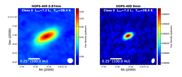
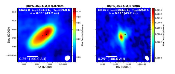
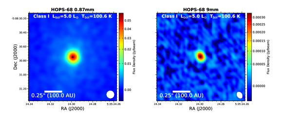
Figure 3: Example images from ALMA (left) at 0.87 mm and the VLA (right) at 9 mm toward selected sources. The top row shows HOPS-409, a Class 0 protostar with an apparent resolved disk at 0.87 mm and 9 mm. HOPS-361-C, a high-luminosity Class 0 source, is shown in the middle row and appears disk-like at 0.87 mm. However, HOPS-361-C is resolved into a close binary system by the VLA at 9 mm. The brighter source also exhibits an extended free-free jet at this wavelength. HOPS-68, a Class I source, is shown in the bottom row and appears compact and only marginally resolved at both 0.87 mm and 9 mm. The synthesized beams are drawn in the lower right; the typical ALMA synthesized beam is 0$\farcs$1 and the typical VLA beam is 0$\farcs$08. Images for the remaining protostars are shown in Appendix C. A blank panel for the ALMA 0.87 mm or VLA 9 mm panel means that observations were not taken toward that particular protostar with ALMA or the VLA.

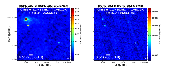
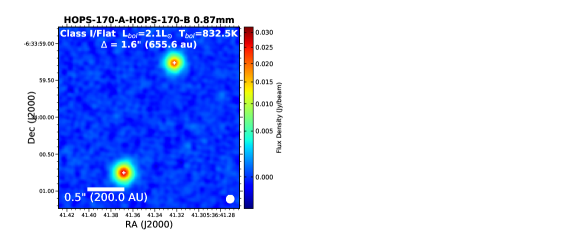
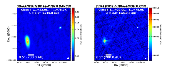
Figure 4: Example images from ALMA (left) at 0.87 mm and the VLA (right) at 9 mm toward selected wide multiple systems. The top row shows HOPS-182 (also known as L1641N), which is made up of a close and wide multiple system. The brighter sources, HOPS-182-A and -B both appear resolved at 0.87 mm and 9 mm. A binary Class I source, HOPS-170, is shown in the middle panel, these sources both show apparent resolved disks that are likely face-on. HH111mms is shown in the bottom panel, showing the brighter disk-like source with a fainter companion separated by 3″and detected at both wavelengths. Furthermore, the jet from HH111mms is also detected at 9 mm. The synthesized beams are drawn in the lower right, the typical ALMA synthesized beam is 0$\farcs$1 and the typical VLA beam is 0$\farcs$08. Images for the remaining sources are shown in Appendix C. A blank panel for the ALMA 0.87 mm or VLA 9 mm panel means that observations were not taken toward that particular protostar with ALMA or the VLA.

We show ALMA and VLA images toward a representative subset of protostars in Figures 3 and 4, while images of the full complement of detected sources are shown in Appendix C. The ALMA 0.87 mm images show extended dust emission that appears well-resolved and disk-like for many protostars, while many others show marginally-resolved and/or point-like emission. Our observations zoom in on the innermost regions of the protostars, resolving the scales on which disks are expected to be present (Tobin et al., 2012; Segura-Cox et al., 2016; Andrews et al., 2009; Hennebelle et al., 2016). Thus, for simplicity we refer to the resolved and unresolved continuum structures observed toward these protostars as disks, despite their Keplerian nature not being characterized in these observations. Seven Class 0 protostars may contain a large contribution from an envelope; we will discuss these in Section 4.5.

Some protostars in the sample exhibit close multiplicity on scales less than 1$\farcs$25 (500 au), and many of these close multiple systems can be seen in the individual panels shown in Figure 3 and Appendix C; some of these systems contain multiple resolved disks in a single system. Other protostars in the sample exhibit multiplicity on scales greater than 1$\farcs$25 (500 au), and those systems are shown in images with a larger field of view in Figure 4. We only show neighboring sources for separations less than 11″, such that they are detectable within the ALMA field of view at 0.87 mm. The multiplicity properties of the protostars, such as the distribution of separations and multiplicity frequencies, are not discussed further here and will be published in a forthcoming paper. Throughout the paper, it is useful to separate the sample into the full sample and non-multiple sample. Non-multiples refer to any system that does not have an ALMA- or VLA-detected companion within 10,000 au.

We consider each detected source, whether it is part of a multiple system or not, individually for the measurement of flux densities, computation of mass estimates, and radii measurements from Gaussian fitting. There are many cases where the companion protostars are close enough that they were not resolved in previous infrared observations from the HOPS program (Furlan et al., 2016) and Spitzer surveys of the region (Megeath et al., 2012). In those instances, we assume that the measurements of L_bol and T_bol apply to both components of the protostar system because they are embedded within a common protostellar envelope and there is no way to reliably determine the luminosity ratio of the presumed individual protostars associated with the compact dust emission from their disks (Murillo et al., 2016). Tables 2 and 4 document the observed fields and protostars associated with them, along with their corresponding L_bol, T_bol, and distance measurements for ALMA and the VLA, respectively. Tables 6 and 7 list the source positions, fields, flux densities, and orientation parameters derived from Gaussian fitting from the ALMA and VLA data, respectively. The derived properties of each source from the ALMA and VLA flux densities and sizes determined from Gaussian fitting are given in Table 8. We followed the data analysis procedures outlined in Section 2.4 to translate our flux densities and source sizes into protostellar dust disk masses and radii. We also provide the spectral indices from 0.87 mm to 9 mm and the in-band spectral indices determined from the VLA data alone.

The comparable resolution of both the ALMA and VLA images enables us to compare the structure observed at a factor of 10 difference in wavelength. In many instances, the ALMA images appear significantly more extended than the VLA images, as shown in Figures 3 and 4, and Appendix C. This may be indicative of structure whose emission has a wavelength dependence. The VLA observations at 9 mm are typically dominated by dust emission (Tychoniec et al., 2018), but there are instances where free-free emission from jets (Anglada et al., 1998) can contribute significantly to the flux density at 9 mm. This emission can be compact and point-like, or it may be extended in the jet direction (see an example in Figures 3 and 4). The emission at 9 mm can be characterized by the spectral index calculated within the Ka-band. Values greater than 2 likely reflect a dominant component of dust emission, while values less than 2 require free-free emission to explain the observed flux density.

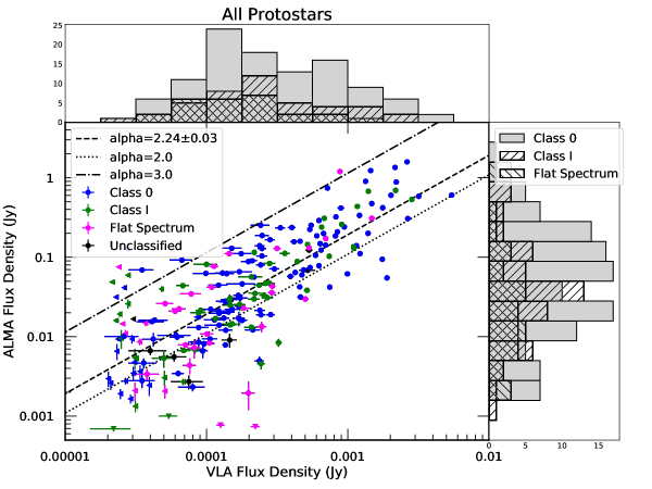
Figure 5: Plot of ALMA 0.87 mm flux density versus VLA 9.1 mm flux density in log-log space. The observational class of the sources are denoted by color where Class 0 protostars are blue, Class I protostars are green, and Flat Spectrum sources are magenta; unclassified sources are black. A strong correlation between the ALMA and VLA flux densities is present, and a constant spectral index can fit the correlation with a spectral index ($\alpha$) $\alpha$ = 2.24$\pm$0.03 (ignoring upper limits). We also plot the line representing $\alpha$ = 2, points below this line require additional free-free emission to explain their shallow spectral slopes. Most sources have $\alpha$ between 2 and 3, consistent with optically thick to optically thin dust emission. The left pointing or downward pointing triangles denote upper limits for the VLA 9 mm or ALMA 0.87 mm observations, respectively.

We show the flux densities for the ALMA and VLA data plotted together in Figure 5. There is a strong correlation between the 0.87 mm and 9 mm flux densities that in log-log space is fit with a constant spectral index ($\alpha$) of 2.24$\pm$0.03 using scipy. This indicates that the emission at the two wavelengths is tracing a similar process, likely dominated by dust emission. Deviations from the relationship are evident; excess emission at 9 mm indicates a large contribution from free-free emission (or high optical depth at 0.87 mm), and excess emission at 0.87 mm indicates that there is less flux at 9.1 mm than expected from the same emission process.

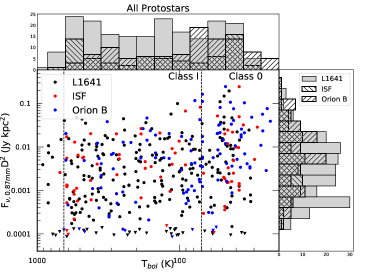
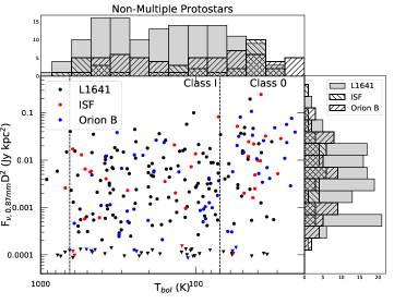
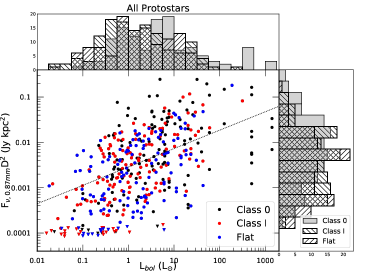
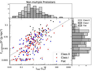
Figure 6: Comparison of 0.87 mm flux densities to T_bol (top panels) and L_bol (bottom panels); the flux densities are multiplied by the square of their distance in kpc to remove scatter due to different distances within the region. The left panels show the full survey sample with a corresponding measurement of L_bol and T_bol, while the right panels show only the non-multiple sample. The colorization and histograms associated with the top panels separates the sources by their regions (black: L1641 and southern ISF, red: Northern ISF, blue: Orion B). In the bottom panels, the colors and associated histograms separate the sources by class; black corresponds to Class 0 protostars, red corresponds to Class I protostars, and blue corresponds to Flat spectrum protostars. Upper limits are denoted as downward facing triangles. The lines in the lower panels are the fits to the 0.87 mm flux densities versus L_bol, for the full sample (left panel) we find $F_{\nu}$D² $\propto$ L${}_{bol}^{0.4\pm 0.04}$ and for the non-multiple sample (right) we find $F_{\nu}$D² $\propto$ L${}_{bol}^{0.61\pm 0.05}$. The vertical lines in the top panels denote the separations between Class 0 and Class I (70 K) and Class I and Class II (650 K).

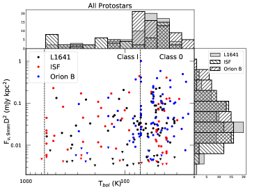
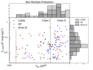
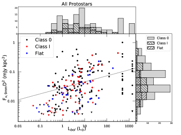
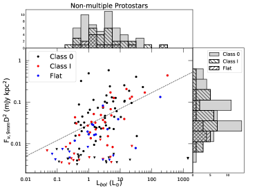
Figure 7: Same as Figure 6, but comparing the 9 mm flux densities. The lines in the lower panels are the fits to the 9 mm flux densities versus L_bol, for the full sample (left panel) we find $F_{\nu}$D² $\propto$ L${}_{bol}^{0.2\pm 0.03}$ and for the non-multiple sample (right) we find $F_{\nu}$D² $\propto$ L${}_{bol}^{0.38\pm 0.07}$.

The observed flux densities at 0.87 mm and 9 mm are compared to L_bol and T_bol of each protostellar system in Figures 6 and 7. Due to the differences in estimated distance toward each protostellar system, we multiply the flux densities by the square of the distance in kpc, yielding a luminosity at the observed wavelengths. The 0.87 mm flux densities span three orders of magnitude independent of class, and the 9 mm flux densities span about 2 orders of magnitude. There are far fewer Class I/Flat Spectrum points at 9 mm due to the selection applied for the VLA observations. It is clear that only a weak trend exists with respect to the observed flux densities and T_bol; Pearson’s R is $\sim$-0.28 for the 0.87 mm flux densities and $\sim$-0.17 for the 9 mm flux densities. This indicates a modest correlation for 0.87 mm flux densities, but a very weak correlation for the 9 mm flux densities. Upper limits were ignored in determining these correlations.

The flux densities at 0.87 mm and 9 mm show clear correlations with L_bol in Figures 6 and 7. We separately plot the full sample including all protostars and the non-multiple sample. We find that the 0.87 mm flux densities are proportional to L_bol^0.41±0.04 and L_bol^0.61±0.05 for the full sample and non-multiple sample, respectively, with Pearson’s R coefficients of 0.50 and 0.64. Similarly, the 9 mm flux densities are proportional to L_bol^0.20±0.3 and L_bol^0.38±0.07 for the full sample and non-multiple sample, respectively, with Pearson’s R coefficients of 0.39 and 0.51. The strong correlations with L_bol for both 0.87 mm and 9 mm are not surprising since higher luminosity will result in warmer dust, which will result in higher flux densities for a given dust mass. The plots only showing the non-multiple sources exhibit cleaner correlations and are likely more robust than the correlations for the full sample. This is because the same bolometric luminosity is adopted for all members of the multiple systems due to a lack of independent luminosity measurements. Analysis of the flux densities as they relate to the underlying dust masses toward the protostellar systems continues in the next subsection.

3.3 Distribution of Protostellar Dust Disk Masses

The integrated flux densities measured with ALMA and the VLA enable the dust disk masses to be estimated under the assumption of an average dust temperature and optically thin dust emission (see Section 2.4 for a more detailed discussion of our methods and assumptions). Note that throughout this section and the rest of the paper, disk masses are given in dust mass (not scaled by an estimate of the dust to gas mass ratio) unless specifically stated otherwise. In the absence of detailed radiative transfer modeling for all the sources (e.g., Sheehan & Eisner, 2017a), the dust disk masses measured from integrated flux densities are the most feasible to compute for a large sample such as the protostars in Orion. The fact that all the protostars in Orion have had their SEDs, L_bol and T_bol characterized enables us to examine trends in the protostellar dust disk masses in the context of these properties. We also note that the dust disk masses we refer to are calculated from the ALMA 0.87 mm continuum, unless specifically stated otherwise; however, we do provide dust disk masses calculated from the VLA 9 mm flux densities in Table 8 for completeness. It is possible that some of the detected emission is from an inner envelope. Also, the continuum mass does not reflect the mass already incorporated into the central protostellar object itself. We consider distributions with multiple sources included (all or full sample) and excluded (non-multiple sample) to isolate the effect(s) of multiplicity on the observed dust disk mass distributions.

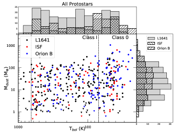
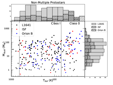
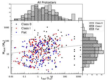
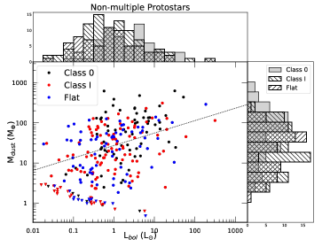
Figure 8: Comparison of dust disk masses to T_bol (top panels) and L_bol (bottom panels). The left panels include the full sample from the survey with a corresponding measurement of L_bol and T_bol, while the right panels show only the non-multiple sample. The colorization and histograms associated with the top panels separates the sources by their regions (black: L1641 and southern ISF, red: Northern ISF, blue: Orion B). In the bottom panels, the colors and associated histograms separate the sources by class; black corresponds to Class 0 protostars, red corresponds to Class I protostars, and blue corresponds to Flat spectrum protostars. Upper limits are denoted as downward facing triangles. The lines in the lower panels are the fits to the dust disk masses versus L_bol, for the full sample (left panel) we find $M_{disk}$ $\propto$ L${}_{bol}^{0.11\pm 0.04}$ and for the non-multiple sample (right) we find $M_{disk}$ $\propto$ L${}_{bol}^{0.31\pm 0.05}$. The vertical lines in the top panels denote the separations between Class 0 and Class I (70 K) and Class I and Class II (650 K).

We examine the protostellar dust disk masses with respect to T_bol and L_bol in Figure 8. We see in Figure 8 that there is significant scatter in the dust disk masses as a function of T_bol for the full sample and also non-multiples. Given the scatter and lack of clear relation between T_bol and protostellar dust disk mass, we calculated the median dust disk masses for Class 0, Class I, and Flat spectrum sources. For the full sample, we find median dust disk masses of 25.7, 15.6, and 13.8 M_⊕, respectively, calculated from sample sizes of 133, 150, and 132 systems in each class, respectively. If we only consider non-multiple sources, then we find median dust disk masses of 52.5, 15.2, and 22.0 M_⊕, respectively, calculated from sample sizes of 69, 110, and 79 systems in each class, respectively. The median dust disk masses for all and non-multiple protostars include upper limits in the calculation. The median masses for the different classes are also listed in Table 9. While there is a trend of lower dust disk mass with evolution, the amplitude of this trend is much smaller that the two orders of magnitude spread in dust disk masses for a given class (see also Segura-Cox et al., 2018). We examine the dust disk mass trends with respect to protostellar class in more detail in the following paragraphs.

The relationship between dust disk mass and L_bol is shown in Figure 8. Such a dependence for protostars could be analogous to the M_∗ - M_disk relationship for Class II YSOs where M_disk $\propto$ M${}_{*}^{1.8}$ (e.g., Ansdell et al., 2016). L_bol is the closest proxy for protostar mass available, but this is a relatively poor proxy due to a substantial (and unknown) fraction of luminosity coming from accretion (Dunham et al., 2014). We fit a linear slope in log-log space to the M_disk versus L_bol plot for the sample including all sources and find that M_disk $\propto$ L_bol^0.11±0.04, with a Pearson’s R correlation coefficient of 0.16, indicating a very weak correlation (Wall, 1996). For a sample limited to non-multiple sources, we find M_disk $\propto$ L_bol^0.31±0.05 and calculate a Pearson’s R correlation coefficient of 0.34, indicating a moderate correlation. We note, however, that by scaling the average dust temperature by L_bol^0.25 we have removed much of the apparent luminosity dependence on the dust disk mass (see previous section for relations with flux densities only), and the remaining correlation could still be affected by the adopted dust temperatures.

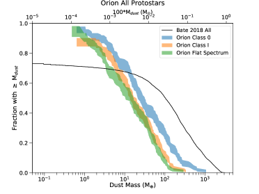
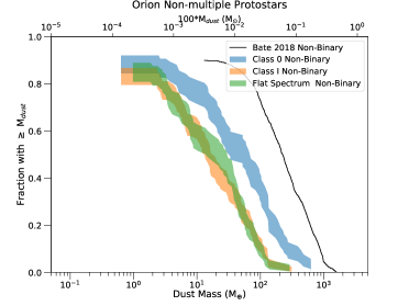
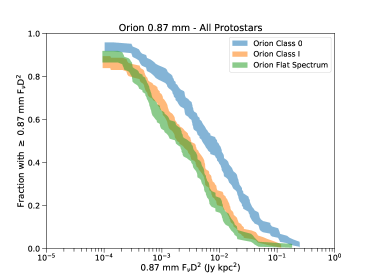
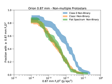
Figure 9: Cumulative distributions of dust disk masses (top row) and 0.87 mm flux densities multiplied by their distance in kpc squared (bottom row) within the Orion sample. The left panels show the full sample, while the right panels only show the non-multiple sample. Class 0 dust disk masses are drawn with a blue shaded region, Class I dust disk masses are drawn with an orange shaded region, Flat Spectrum dust disk masses are drawn with a green shaded region. The Class 0 dust disk masses clearly have their distribution shifted toward higher masses, while there is less difference between the Class I and Flat Spectrum dust disk masses; this is true for the full and non-multiple samples. The full and non-multiple samples are also compared to the dust disk masses derived from the large-scale simulations of Bate (2018). The mass distributions from the simulations have a systematic shift toward higher masses in both the full and non-multiple samples. Statistical comparisons between the dust disk masses of each class is discussed in the text. The distributions of 0.87 mm flux densities, from which the dust disk masses are derived, show the same overall trend of higher 0.87 mm flux densities for Class 0. The Class I 0.87 mm flux densities are systematically higher than Flat Spectrum sources for the population of all protostars, but have substantial overlap for the non-multiple sample.

The dust disk mass distributions can be more clearly examined as cumulative distributions shown in Figure 9. The plots were constructed using survival analysis and the Kaplan-Meier estimator as implemented in the Python package lifelines (Davidson-Pilon et al., 2019). We make use of the left censored fitting functions that account for upper limits derived from the non-detections. The width of the cumulative distributions plotted represents the 1$\sigma$ uncertainty of the distribution. The larger median masses of Class 0 disks both for the full sample and non-multiple sample are evident in Figure 9.

To statistically compare the distributions, we used the log rank test as implemented in lifelines. We found that the distribution of Class 0 masses is inconsistent with being drawn from the same distribution as the Class I and Flat spectrum sources at $>$99% confidence (p$<$0.01) for both the samples considering all sources and non-multiples. However, the differences between the Class I and Flat spectrum sources are not statistically significant. Thus, the Class I and Flat Spectrum mass distributions are consistent with being drawn from the same sample. Note that we obtained consistent results from the Anderson-Darling test (Scholz & Stephens, 1987) on the cumulative distributions alone without considering the upper limits. We list the p-values from the sample comparisons in Table 10 and also provide the p-values from the Anderson-Darling tests when conducted.

These cumulative dust disk mass distributions can also be approximated as a log-normal cumulative distribution function (CDF), which can be directly translated to a Gaussian probability density function (PDF), as has been demonstrated by Williams et al. (2019). To determine the mean and standard deviation of the Gaussian PDF, we fit the cumulative distributions derived from lifelines with the survival function (defined as 1 - Gaussian CDF) using the curve_fit function within scipy. To calculate the 1$\sigma$ uncertainties, instead of adopting the standard error from the fit, we performed the same fit on the 1$\sigma$ upper and lower bounds of the cumulative dust disk mass distributions from the survival analysis and adopted the relative values of these parameters as the uncertainties. We note, however, that the observed distributions are not precisely Gaussian, so the parameters derived from these fits may not be completely accurate, nor their uncertainties.

The mean dust disk masses for Class 0, I, and Flat Spectrum systems are 25.9${}^{+7.7}_{-4.0}$, 14.9${}^{+3.8}_{-2.2}$, 11.6${}^{+3.5}_{-1.9}$ M_⊕, respectively, for the full distributions considering all systems. Limiting the sample to non-multiple systems we find mean dust disk masses of 38.1${}^{+18.9}_{-8.4}$, 13.4${}^{+4.6}_{-2.4}$, and 14.3${}^{+6.5}_{-3.0}$ M_⊕, respectively. These mean values of the distributions are quite comparable to the median dust disk masses for the same distributions, and the uncertainties on the means further demonstrate that the Class 0 dust disk masses are systematically larger than those of Class I and Flat Spectrum and differ beyond the 1$\sigma$ uncertainties of the mean masses. The mean masses of the Class I and Flat Spectrum protostars are consistent within the uncertainties, a further indication that there is not a significant difference between the disk masses in these two classes.

3.4 Distribution of Protostellar Dust Disk Radii

We utilize the deconvolved Gaussian 2$\sigma$ radius from the fits to the continuum images as a proxy for the radius of the continuum sources, enabling us to characterize the disk radii in a homogeneous manner (see Section 2.4). These values are provided in Table 8 for both the ALMA and VLA measurements. However, we only make use of the ALMA measurements in this analysis due to the 0.87 mm continuum emission having a greater spatial extent that can more accurately reflect the full radius of the disk. The VLA continuum emission is often compact and point-like, even toward protostars with apparent resolved disks at 0.87 mm; see Figures 3 and 4 as well as Segura-Cox et al. (2016, 2018).

Visual inspection of the Gaussian fits reveals that there are often residuals outside the Gaussian model. This affects the larger disks (R $>$ 50 au) more than the compact ones, and our measured radii will be systematically underestimated in some cases. The determination of deconvolved Gaussian 2$\sigma$ radii can also be subject to some systematics. If the S/N is high enough, then a source smaller than the beam can be deconvolved from it under the assumption that the underlying source structure is also Gaussian. Trapman et al. (2019) showed that if the peak S/N of dusty disk emission was $>$10, the disk radius could be recovered reasonably well. Those authors, however, were using the curve of growth method rather than Gaussian fitting. Our sample typically has modest S/N, between 20 to 100, and we regard deconvolved radii significantly smaller than half size of the synthesized beam (0$\farcs$05, 20 au) as being possibly unreliable. In our analysis, we only include sources with strong enough emission such that an estimate of the deconvolved size could be made. Weak sources that required their major axis, minor axis, and position angle to be fixed to the synthesized beam are not included in these plots. We do, however, tabulate the fits that indicate a deconvolved radius smaller than 10 au even though these may be too small to be reliable.

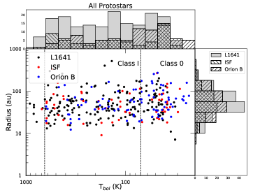
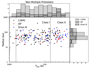
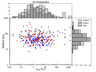
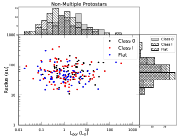
Figure 10: Comparison of protostellar disk radii to T_bol (top panels) and L_bol (bottom panels). The accompanying histograms in the top panels separate the sample by their region and in the bottom panels the sample is separated by class. The colorization and histograms associated with the top panels separates the sources by their regions (black: L1641, red: integral-shaped filament [ISF], blue: Orion B). In the bottom panels, the colors and associated histograms separate the sources by class; black corresponds to Class 0 protostars, red corresponds to Class I protostars, and blue corresponds to Flat spectrum protostars. The left panels show the full sample with a corresponding measurement of L_bol and T_bol, while the right panels show only non-multiple sample. There is no strong correlation between disk radii and T_bol or L_bol.

We compare the disk radii to T_bol in the top panels of Figure 10. The median radii for the Class 0, Class I, and Flat Spectrum sources are 48, 38, and 31 au, respectively, for the full sample, and 55, 37, and 38 au, respectively, for the non-multiple sample; we also list these values in Table 9. The amplitude of this trend is small given the order of magnitude scatter within each class. Thus, the Class 0 sources have a tendency for larger radii compared to the Class I and Flat Spectrum sources, and non-multiple sources also tend to have larger disks. The sensitivity of the current observations may not be sufficient for detecting circumbinary emission (disks), however. We do include the deconvolved radii calculated for the unresolved and marginally resolved disks, which may artificially inflate median measured disk radii if the disks are significantly smaller than their upper limits. Even if a disk radius measured from the deconvolved Gaussian is below our expected measurement limit of 10 au, we do not plot it as an upper limit and leave it at its measured value. Furthermore, we do not account for non-detections when calculating the median radii. We also compare the distribution of radii to L_bol; again, there is no clear trend, and both high- and low-luminosity sources can have large and small radii. However, the non-multiple sources with luminosity greater than 100 L_☉ have radii of $\sim$120 au, but only for a sample of 2.

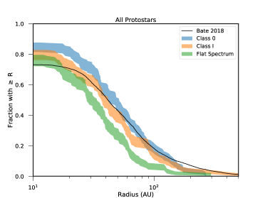
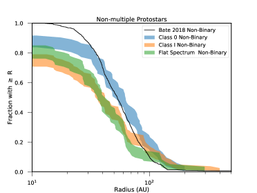
Figure 11: Cumulative distributions of disk radii within the Orion sample. The left panel shows the full sample, while the right panel only shows the non-multiple sample. Protostars with a measured dust disk radius that is $\leq$ 10 au or did not have a measurement due to low S/N is considered an upper limit for the purposes of the survival analysis produced by the lifelines package. Class 0 protostars are drawn with a blue shaded region, Class I protostars are drawn with an orange shaded region, Flat Spectrum sources are drawn with a green shaded region. The Class 0 sources clearly have their distribution shifted toward larger radii; this is more evident in the case of non-multiple sources. The distribution of Class I radii is slightly higher than the Flat spectrum radii for the full sample, but when only considering non-multiple systems, there is very little difference in the distributions. The full sample and non-multiple samples are also compared to the disk radii derived from the large-scale simulations of Bate (2018). The radii distributions from the simulations are comparable to the Class 0 and Class I disk radii for both the full sample and non-multiple cases.

The disk radii distributions are also examined as cumulative distributions using survival analysis and the Kaplan-Meier estimator as implemented in the Python package lifelines and shown in Figure 11. Here the systematically larger sizes of Class 0 disks are evident by eye. To establish the statistical significance of these differences, we compare these distributions quantitatively using a log rank test, similar to how we compared the distributions of dust disk masses. Considering all sources (multiple and non-multiple), we compared Class 0 vs. Class I, Class 0 vs. Flat Spectrum, and Class I vs. Flat Spectrum, and the likelihood that these samples are drawn from the same distribution are 0.63, 0.0002, and 0.003, respectively. Thus, there is no statistical evidence that the Class 0 and Class I radii distributions are drawn from different distributions. However, the distributions of Class 0 and Flat Spectrum and Class I and Flat Spectrum disk radii are inconsistent with being drawn from the same parent distribution from the log rank test. A summary of the sample comparison probabilities is provided in Table 10.

We then compared the radii distributions for the non-multiple sources, and we conducted the same comparisons as in the previous paragraph. These were Class 0 vs. Class I, Class 0 vs. Flat Spectrum, and Class I vs. Flat spectrum, which have likelihoods of being drawn from the same parent distribution of 0.59, 0.04, and 0.13, respectively. Thus, at the 99% confidence level the distributions of disk radii are all consistent with having been drawn from the same sample. However, looking at Figure 11 we would expect the Class 0 sample to not be consistent with having been drawn from the same distribution as the Class I and Flat Spectrum samples. This counter-intuitive result could be caused by the inaccuracy of the log rank test when the cumulative distributions cross (Davidson-Pilon et al., 2019), as the Class 0 sample does with the Class I and Flat Spectrum samples. Furthermore, the uncertainty width shown in Figure 11 is the 1$\sigma$ width, and within 2$\sigma$ the distributions would overlap significantly more. As an additional test we performed an Anderson-Darling test on the distributions, finding results consistent with the log rank test.

To characterize the distributions of disk radii further, we fit a Gaussian CDF to the cumulative distributions of disk radii from the survival analysis in the same manner as we fitted the Gaussian CDF to the dust disk mass distributions. This enabled us to derive mean radii and widths of the log-normal distributions with associated uncertainties. The mean radii for the full sample of Class 0, Class I, and Flat Spectrum protostars are 44.9${}^{+5.8}_{-3.4}$, 37.0${}^{+4.9}_{-3.0}$, and 28.5${}^{+3.7}_{-2.3}$ au, respectively, and the mean radii for non-multiple sample are 53.7${}^{+8.4}_{-4.2}$, 35.4${}^{+6.1}_{-3.5}$, and 36.0${}^{+5.9}_{-3.2}$ au, respectively. These properties of the distributions are listed in Table 9. The consistency (or lack thereof) of the mean radii when compared between classes are in line with the results from the log rank tests, except for the Class 0 to Class I disk radii for the non-multiple sample, where the log-rank test indicates that they are consistent with being drawn from the same parent distribution.

The mean radii from the Gaussian PDFs indicate that the distributions of disk radii are not extremely different between Class 0, Class I, and Flat Spectrum. For the full sample, only the Class 0 and Class I distributions of disk radii are consistent with being drawn from the same sample; the Class 0 and Flat Spectrum and Class I and Flat Spectrum distributions are inconsistent with being drawn from the same sample. The radii distributions for the non-multiple samples, however, are all consistent with having been drawn from the same samples (see Table 10).

The distributions in Figure 11 also clearly show that disks substantially larger than the median radii exist for protostars of all classes. However, taking 50 au as a fiducial number to define the qualitative distinction between large and small disks, $\sim$46% (N=61) of Class 0, $\sim$38% of Class I (N=57), and $\sim$26% (N=35) of Flat Spectrum disks have radii larger than 50 au. These percentages are calculated from (N(R$\geq$50 au)/(N(continuum sources)+N(non-detections)) (Table 5). If only non-multiples from each class are considered, the percentage of dust disks with radii $>$ 50 au are 54% (N=37), 38% (N=42), and 37% (N=29) for Class 0, Class I, and Flat Spectrum, respectively. These percentages are calculated from (N(R$\geq$50 au, non-multiple)/(N(non-multiple systems)+N(non-detections)).

3.5 Distribution of Protostellar Dust Disk Masses versus Radius and Inclinations

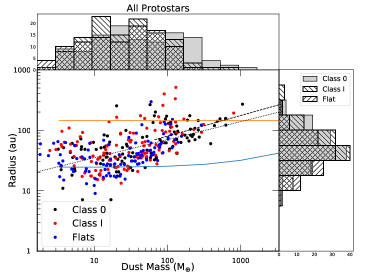
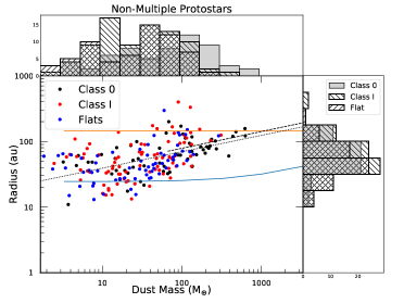
Figure 12: Comparison of disk radii versus dust disk mass for the full sample (left) and the non-multiple sample (right). The Class 0 disks are represented by black points, the Class I disks by red points, and Flat spectrum disks by blue points. There is a clear correlation in that the sources with larger disk radii have higher masses. Smaller disks could have higher masses that cannot be measured due to high optical depth. Upper limits are not shown because an upper limit on disk radius is unphysical if there is not a detection. The solid lines are the analytic prescriptions for disk radii vs. dust disk mass from Hennebelle et al. (2016). The lower line is for the case of disks formed in the presence of magnetic fields, while the upper line is for the case of a disk formed in the hydrodynamic limit; see section 4.6.2. The dotted and dashed lines in the right and left panel are fits to the correlation between radius and mass; the dotted lines only consider masses $>$33 M_⊕. The relationships are all comparable to R $\propto$ M${}_{disk}^{0.3}$, see Section 3.5 and 4.6.2 for further detail.

Lastly, we examine the relationship between dust disk mass and radius for both the full sample and non-multiple systems. Figure 12 shows that below $\sim$30 M_⊕, there is no apparent relation between dust disk mass and disk radius. In both panels of Figure 12, the radii are clustered around 35 au for dust disk masses less than $\sim$30 M_⊕, and there is a large spread in radius for a given dust disk mass. There is also not a clear distinction between the classes with all three spanning the same range of parameter space in Figure 12.

We do find that for masses greater than 30 M_⊕, there is an apparent trend of increasing radius with mass. We fit the correlation between disk radii and mass using scipy. If we include all the masses and radii in the fit, we find that R $\propto$ M_disk^0.3±0.03 (Pearson’s R = 0.54); if we only fit masses greater than 67 M_⊕, then R $\propto$ M${}_{disk}^{0.34\pm 0.09}$ (Pearson’s R = 0.37). These fits are plotted in Figure 12 as dotted and dashed lines, respectively. If we instead limit the sample to non-multiple systems, then we find that R $\propto$ M_disk^0.25±0.03 (Pearson’s R = 0.49) and R $\propto$ M_disk^0.26±0.1 (Pearson’s R = 0.27) for the same ranges of dust disk masses used for the full sample, respectively. As a limiting case, a sample of optically thick disks with a variety of radii would have a disk radius that increases with the square-root of the dust disk mass. For both fits, the relationship is more shallow than this simple case; this indicates that the disks we observe should not be optically thick at all radii.

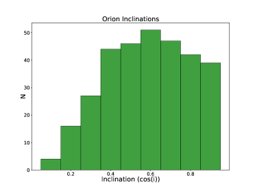
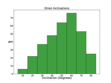
Figure 13: Histogram of inclinations derived from the deconvolved major and minor axes from Gaussian fitting in cos($i$) (left panel) and degrees (right panel). A completely random distribution would be flat in cos($i$) but peaked at 60°. We see that the distribution in cos($i$) starts to drop at values lower than 0.4, which is likely because the deconvolved minor axes fit for sources close to edge-on ($\sim$90°; cos($i$)= 0) are generally overestimated due to the resolution of the survey.

We also estimate the inclination of the protostellar systems, under the assumption of circular symmetry using the measurements of the protostellar disk radii from the deconvolved semi-major and semi-minor axis of the Gaussian fits. We show the histogram of inclinations in Figure 13 both in terms of cos($i$) and degrees; an inclination of 90° refers to viewing a disk edge-on, while 0° refers to viewing a disk face-on. A completely random distribution of inclinations should have a flat histogram with equal numbers in each bin of cos($i$). However, we can see that the histogram of cos($i$) declines at low values which corresponds to high inclinations (near edge-on). The histogram of inclinations in degrees is shown in the right panel of Figure 13, and for a flat distribution of cos($i$), reflecting a random distribution of inclinations, the average value should be 60°. The median and mean values of cos($i$) are 0.596 and 0.601, respectively, corresponding to 53.4° and 53.1°. This average value is less than 60° due to the lack of sources computed to have high inclinations. However, we do not think that this difference is significant because looking at the continuum images in Figure 3 and 5 and Appendix C, there are sources that appear to be oriented near edge-on. The reason their inclinations do not compute to edge-on is because this requires deconvolved minor to major axis ratios very near to zero. Furthermore, the disks are known to have a finite thickness to their dust emission (Lee et al., 2017); this, combined with finite resolution, will lead to the distribution being biased against edge-on sources.

3.6 Regional Comparison of Disk Properties

The Orion star-forming region, as highlighted in Figure 1, encompasses much more than just the region around the Orion Nebula. There are two giant molecular clouds in Orion denoted A and B. The Orion A molecular cloud encompasses the molecular emission south of $\sim$-4.5° declination, and we consider two regions within Orion A with distinct properties: the northern half of the Integral-Shaped Filament (ISF) and L1641. We consider protostars between -4.5° and -5.5° declination as part of the northern ISF and protostars south of -5.5° as part of the southern ISF and L1641. The ISF extends to $\sim$-6°, and the southern ISF between -5.5° and -6° has a YSO density similar to L1641, so we consider them together.

The northern half of the ISF is located between the Trapezium and NGC 1977 and has a high spatial density of protostars and high-density molecular gas (Peterson et al., 2008; Megeath et al., 2012; Stutz & Kainulainen, 2015; Stutz & Gould, 2016). This region is also referred to as Orion Molecular Cloud 2/3 (OMC2/3) and has its protostellar content well-characterized (e.g., Furlan et al., 2016; Tobin et al., 2019, Díaz-Rodríguez in prep.). The central portion of the ISF is located behind the Orion Nebula, where the SEDs of YSOs do not extend beyond 8 µm due to saturation at longer wavelengths. In contrast to the northern ISF, the southern ISF and L1641 have a much lower spatial density of protostars (Allen et al., 2008; Megeath et al., 2012).

We then consider protostars located north of -4.5° as part of Orion B, which itself contains several sub-regions that we consider together: the Horsehead, NGC 2023, NGC 2024, NGC 2068, NGC 2071, L1622, and L1617 (Megeath et al., 2012). Note that we do not have sources in our sample between declinations of -02:21:17 and -4:55:30, so the exact boundary in declination between Orion A and Orion B is not important (Figure 1). To sample a variety of environments with a reasonably large number of protostars in each sub-sample, we compared L1641 and southern ISF (low spatial density), to the northern ISF (high spatial density), and Orion B (low spatial density). We note that both L1641 and Orion B contain regions of high protostellar density, but compared to the northern ISF they have low overall spatial density of protostars (Megeath et al., 2016).

We examined the dust disk masses within L1641 and Southern ISF, the Northern ISF, and Orion B, finding median values of 14.7, 15.2, and 24.3 M_⊕, respectively, for the full sample with respective sample sizes of 235, 76, and 113 protostars, within each region. Limiting the analysis to the non-multiple sources, the median dust disk masses are 23.7, 18.7, and 28.3 M_☉, respectively, with respective sample sizes of 165, 39, 63 protostars (see also Table 9). The calculations of median mass measurements for each region include non-detections. While we find the differences in median masses between all sources and non-multiples reported earlier, there is no significant variation between the regions. A log rank test performed on the distributions reveals that the mass distributions for non-multiple sources are consistent with having been drawn from the same sample. cumulative distributions with a Gaussian CDF in the same manner as described for the full dust disk mass distributions. When comparing the means of these distributions, only Orion B vs. L1641 for the full sample differs by more than 1$\sigma$ (but less than 2$\sigma$); these values are listed in Table 9. A summary of the statistical tests and sample sizes are given in Table 10.

We also examined the disk radii within L1641 (N=181), the ISF (N=60), and Orion B (N=93), finding median radii of 45.6, 38.0, and 39.7 au, respectively, for the full sample. Limiting the analysis to the non-multiple sources, we find median radii of 54.5, 40.4, and 48.2 au, respectively, with respective sample sizes of 127, 31, and 47 protostars. The number of protostellar disks included in each region is different with respect to the number used for mass calculations, because we excluded non-detections and the low S/N sources that required Gaussian parameters to be set equivalent to the synthesized beam. The trend of larger disk radii in non-multiple systems is again evident in these median values, but there are not significant differences between regions. We confirmed that the radii distributions between the different regions were consistent using a log rank test for all sources and non-multiple sources. The distributions are consistent with being drawn from the same sample (see Table 10). Moreover, the mean disk radii for these regions, derived from fitting a Gaussian to the cumulative distributions, are consistent within their 1$\sigma$ uncertainties.

This analysis demonstrates that within the limits of our dust disk mass and radius measurements, the properties of protostellar disks do not show statistically significant differences between sub-regions within the Orion molecular clouds. We do not draw a direct comparison to the disks within the Trapezium in this section because we targeted very few protostars located within the Orion Nebula itself, under the influence of the ionizing radiation from the massive stars there. This is due in part to these sources not being targeted by the Herschel Orion Protostar survey because of the bright emission from the nebula in the mid- to far-IR, and hence the sample of protostars toward the Orion Nebula is potentially highly incomplete and poorly characterized. The Class II disks within the Orion Nebula Cluster, on the other hand, have been studied with ALMA by Mann et al. (2014) and Eisner et al. (2018).

4 Discussion

The large sample of protostellar disks detected and resolved in our survey toward the Orion protostars enables an unprecedented comparison of protostellar disk properties to SED-derived protostellar properties. The observed relation of dust disk masses and radii to evolutionary diagnostics such as L_bol and T_bol enables a better understanding of how disk evolution is coupled to protostellar evolution. While the disk radii and masses do not strongly depend on any evolutionary diagnostic, the protostars overall have lower dust disk masses and smaller dust disk radii with increased evolution. The large amount of scatter in the relations may point toward differences in the initial conditions of star formation (core mass, turbulence, magnetic fields, net angular momentum, etc.). It is important to emphasize that the protostellar classification schemes are imprecise tracers of evolution due to the viewing angle dependence of T_bol and the SED slope, but the scatter within a protostellar class is much too large to be attributed to classification uncertainty alone (e.g., see Figure 7 of Fischer et al., 2017). Furthermore, we still lack specific knowledge of the most important protostellar property, the current mass of the central protostar. Bolometric luminosity can be used as a proxy for stellar mass, but it is a very poor proxy with limited relation to the underlying protostellar mass (Dunham et al., 2014; Fischer et al., 2017). We explore these relationships in greater detail in the following section and compare them to predictions of models.

4.1 Protostellar Dust Disk Masses

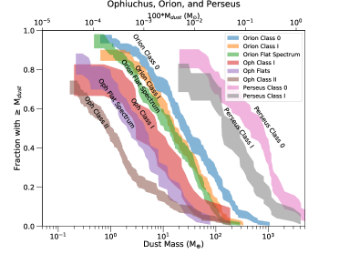
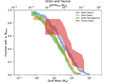
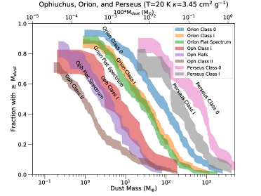
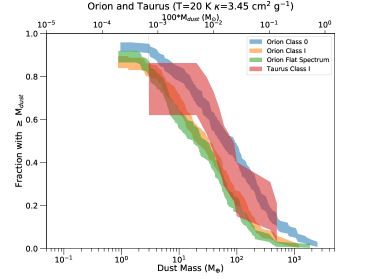
Figure 14: Cumulative distributions of dust disk masses within the Orion sample relative to other protostellar disk surveys; Perseus and Ophiuchus in the left panel and Taurus in the right panel. The top panels use the dust opacity and temperature scaling with luminosity defined in Section 2.4, while the bottom panels use the same dust opacity law as the Ophiuchus/Class II disk samples and a temperature of 20 K. This distribution is for all Orion protostars regardless of multiplicity because the other samples do not exclude multiples. Perseus appears to have higher masses than Orion, but this is likely due to an underestimate of the dust opacity at 9 mm, leading to an overestimate of the masses. The Class I and Flat Spectrum sources from Ophiuchus are significantly lower in mass with respect to Orion. The Class I protostars from Taurus (right panel) are in reasonable agreement with Orion, despite the different methods and small sample.

To better understand the evolution of dust disk masses from the protostellar to the Class II phase, it is essential to compare them to the measured distributions of dust disk masses for both other protostellar samples and Class II disk samples. We first compare the distribution of Orion protostellar dust disk masses to those of the Perseus protostellar disk sample from Tychoniec et al. (2018), the Ophiuchus sample from Williams et al. (2019), and a sample of Taurus Class I disks from Sheehan & Eisner (2017a). It is clear from Figure 14 that the Orion protostellar disks lie directly between the Perseus and Ophiuchus disk mass distributions. The Taurus protostellar disks are reasonably consistent with Orion, despite the smaller sample size and the masses derived from radiative transfer modeling and different dust opacities. The mean and median dust disk masses for the various samples are provided in Table 9.

The protostars within the Perseus sample may be similar in protostellar content to the Orion sample, since it was also an unbiased survey of the entire region, just with a smaller sample and lacking as many high-luminosity sources. However, the median dust disk mass is 25$\times$ larger than the median for Orion (or $\sim$5$\times$ for T=20 K and $\kappa$=3.45 cm² g^-1), but Tychoniec et al. (2018) used the VLA 9 mm data for Perseus, corrected for free-free emission using 4.1 and 6.4 cm data, to calculate their masses. The difference in wavelength and adopted dust opacity introduces a high likelihood of introducing systematic differences to the distribution of the Perseus dust disk masses. They used the Ossenkopf & Henning (1994) dust mass opacity at 1.3 mm (0.899 cm² g^-1) extrapolated to 8 mm by assuming a dust opacity spectral index of 1 and a constant average dust temperature of 30 K. Prior to plotting the Perseus dust disk mass distributions in Figure 14 we adjusted the masses to account for the revised distance of 300 pc to the region (Ortiz-León et al., 2018), and we scaled the dust temperature using L_bol and the same temperature normalization that was used for the Orion protostars (Section 2.4 and Appendix B). However, the dust temperature scaling did not significantly alter the distribution of Perseus dust disk masses. Another study of Perseus dust disk masses was carried out by Andersen et al. (2019) using Submillimeter Array (SMA) data from the Mass Assembly of Stellar Systems and their Evolution with the SMA (MASSES) Survey (e.g., Lee et al., 2016) using lower resolution data ($\sim$3″) to estimate dust disk masses by removing an estimated envelope contribution. We compare the VANDAM Perseus dust disk masses with those from Andersen et al. (2019) in Appendix D, but they similarly find systematically higher dust disk masses with respect to Orion.

Thus, it is unclear if the Perseus protostars really have systematically more massive dust disks. The adoption of a different dust opacity slope could easily bring the distributions into closer agreement. While we do not have complementary observations to longer centimeter wavelengths to enable a more rigorous determination of free-free contamination to the VLA Orion data, we compare our 9 mm dust disk mass measurements to the VANDAM Perseus dust disk mass measurements, 0.87 mm ALMA dust disk mass measurements, and the distributions of 9 mm flux densities in Appendix D. The results indicate Orion at 9 mm is comparable to Perseus at 9 mm, thus pointing to the adopted dust opacity leading to overestimated dust disk masses. A systematic study of the Perseus protostars using ALMA at a comparable spatial resolution, wavelength, and sensitivity to the Orion survey will be necessary to better compare these regions.

In contrast to Perseus, the Orion protostars of all classes have systematically higher dust disk masses than those in Ophiuchus (Cieza et al., 2019), despite similar observing and analysis strategies (Figure 14). Williams et al. (2019) made several different assumptions about dust temperature (adopting a uniform 20 K) and a larger dust opacity (2.25 cm² g^-1 at 225 GHz) assuming $\kappa$ = ($\nu$/100 GHz) cm² g^-1. If we make the same assumptions as Williams et al. (2019) to calculate dust masses, the Orion median masses only increase and are still inconsistent with Ophiuchus (see the bottom panels of Figure 14). This is because the adoption of a 2$\times$ higher dust opacity does lower the masses, but the uniform 20 K temperature cancels out the effect of a higher dust opacity and can significantly raise the dust disk mass for some protostars. In fact, the way to bring the distributions into as close as possible agreement is to adopt the higher mass opacity, but keep higher temperatures that are adjusted for luminosity. But even with this adjustment, the distributions of Class I and Flat Spectrum protostars are still in disagreement by about a factor of 2.

Since the dust disk masses between Ophiuchus and Orion cannot be reconciled by adopting the same set of assumptions, either the protostellar disk properties in Ophiuchus are different from Orion or there is sample contamination in Ophiuchus. Cieza et al. (2019) selected the sample used in Williams et al. (2019) from the Spitzer Cores to Disks Legacy program (Evans et al., 2009), and the YSOs were classified according to their SEDs. Williams et al. (2019) adopted 26 protostars as Class I and 50 as Flat Spectrum. However, McClure et al. (2010) analyzed the region with Spitzer IRS spectroscopy, finding that the 2 to 24 µm spectral slope used by Cieza et al. (2019) performs poorly in Ophiuchus due to the heavy foreground extinction. Thus, McClure et al. (2010) found that out of 26 sources classified as Class I protostars from their 2 to 24 µm spectral slope, only 10 remained consistent with protostars embedded within envelopes when classified using the IRS spectral slope from 5 to 12 µm, which they regarded as more robust because it is less affected by foreground extinction. In addition, van Kempen et al. (2009) examined dense gas tracers toward sources classified as Class I and Flat Spectrum in Ophiuchus, finding that only 17 had envelopes with emission in dense gas tracers. Thus, it is possible that some of the Class I and Flat Spectrum protostars in the Cieza et al. (2019) and Williams et al. (2019) samples are actually highly extincted Class II sources.

However, the dust disk mass distributions as shown indicate that accounting for contamination in Ophiuchus alone will not fully reconcile the disagreement with Orion because the high-mass end of the Ophiuchus dust disk mass distribution is still inconsistent with Orion. This may signify that there is an overall difference in the typical protostellar dust disk masses in Ophiuchus and Orion. One possibility is that the Class I and Flat Spectrum Sources in Ophiuchus could be systematically older than those found in Orion. This is plausible given the relatively small number of Class 0 protostars in Ophiuchus (Enoch et al., 2009) relative to Class I and Flat Spectrum. However, it is also possible that differences in the initial conditions of formation in Ophiuchus versus Orion could result in a different distribution of dust disk masses. What is clear from this comparison of different regions is that it is essential to compare dust disk mass distributions that utilize data at comparable wavelengths and resolution to minimize biases due to the adopted dust opacities, spatial resolution, and differences in the methods used to extract the disk properties.

4.2 Protostellar Dust Disk Masses versus Class II Dust Disk Masses

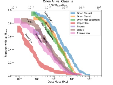
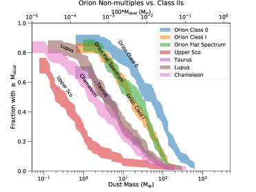
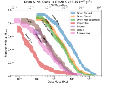
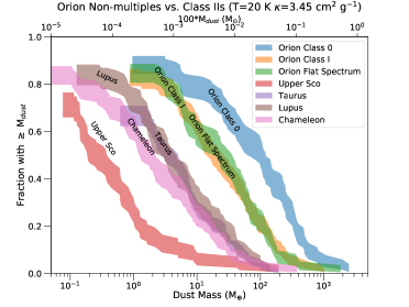
Figure 15: Cumulative distributions of dust disk masses within the Orion sample relative to Class II disk surveys. The top panels use the dust opacity and temperature scaling with luminosity defined in Section 2.4, while the bottom panels use the same dust opacity law as the Class II disk samples and a temperature of 20 K. The left panels show the full sample, while the right panels only show the non-multiple sample. The protostellar sources in Orion all have significantly higher dust disk masses than the more-evolved Class II disks from multiple star-forming regions. This suggests that the protostellar disks may be where planet formation begins, given the significantly larger reservoir of dusty material.

To further understand disk evolution past the protostellar phases, it is essential to compare protostellar disk samples to the more evolved Class II disk samples. The distribution of Orion protostellar dust disk masses is shown in Figure 15 alongside the mass distributions of Class II disks from surveys of different star-forming regions. The Class II disk surveys are reasonably complete and representative in their samples: the Lupus disks are from Ansdell et al. (2016), the Chamaeleon disks are from Pascucci et al. (2016), the Upper Sco disks are from Barenfeld et al. (2016) and the Taurus disks are from Tripathi et al. (2017). We also list the median dust disk masses from the various surveys in Table 9. There are more surveys (even in Orion itself e.g., Eisner et al., 2018; van Terwisga et al., 2019), but to avoid making the comparison plots overly complex, we limited our comparison to some of the most complete surveys.

The Class II dust disk mass distributions shown in Figure 15 have systematically lower masses with increasing age of the stellar population, with Upper Sco being the oldest. We note that these other surveys typically adopt a uniform temperature of 20 K and a dust mass opacity law of $\kappa$=($\nu$/100 GHz)^β, where $\beta$ = 1. Our main results are formulated using a different dust opacity and the assumption of average dust temperatures based on L_bol; however, for comparison we show plots in Figure 15 using the same assumptions as the Class II disk studies.

It is clear that the distribution of protostellar dust disk masses in Orion is systematically higher than the distributions found for Class II disks by a factor greater than 4 (Figure 15), depending on which samples are being compared to Orion. The lower dust masses for Class II disks are particularly important for establishing the feasibility of giant planet formation in the context of the core accretion model (e.g., Pollack et al., 1996). The formation of a 5 to 10 M_⊕ planetary cores built up from the dusty solid material within a disk is required before the gas can be accreted from the disk, enabling the formation of a giant planet (e.g., Hubickyj et al., 2005; Piso et al., 2015). Thus, most Class II disks may not have the requisite raw material within their disks (that can be detected by ALMA) to build up such large solid bodies from scratch, while many of the protostellar disks in Orion (and other regions) have sufficient raw material to form many giant planets within a single system. However, it is possible (perhaps likely) that solids have already grown beyond millimeter sizes in Class II disks, limiting the ability of millimeter/submillimeter observations to detect their emission. Thus, planetesimal formation and perhaps the cores of giant planets may have already formed within the protostellar disks prior to their evolution into Class II disks. Moreover, the disks around pre-main-sequence stars are frequently found to have substructure within them in the form of rings, gaps, cavities, and asymmetries (e.g., Andrews et al., 2018; van der Marel et al., 2019). There have even been indications of such substructures within protostellar disks (Sheehan & Eisner, 2017b, 2018, Segura-Cox et al. in prep.; Sheehan et al. in prep.). While there are multiple theoretical explanations for these structures, the most tantalizing is planet formation.

This means that protostellar disks may better represent the initial conditions for planet formation because they are more likely to have pristine environments where significant dust evolution is just beginning (e.g., Birnstiel et al., 2010). Models of dust evolution indicate that dust grains can grow to cm sizes in the protostellar phase within a few 100,000 yr. Thus, no matter if the full protostellar phase lasts $\sim$500 kyr (Dunham et al., 2014) or the sum of the half-lives ($\sim$222 kyr) (Kristensen & Dunham, 2018), it is possible that Class II disks have already been formed with large dust particles and perhaps even produced planetesimals or planets. Therefore, the dust disk masses around the protostars may provide a more accurate measurement of the amount of raw material available for planet formation.

It is important to highlight that not all samples of Class II dust disk masses follow the trend of systematically decreasing dust disk mass with the stellar population age. Both Ophiuchus and Corona Australis have Class II populations with ages comparable to Lupus and Taurus, but their dust disk mass distributions are systematically lower than Lupus and Taurus. Their mass distributions are similar to that of Upper Sco (Williams et al., 2019; Cazzoletti et al., 2019). Moreover, the Class I and Flat Spectrum dust disk masses in Ophiuchus are lower than those in Orion, possibly pointing to a global phenomenon resulting in lower dust disk masses for all YSO classes in Ophiuchus.

4.3 Protostellar Disk Radii and Their Evolution

Prior to the inclusion of non-ideal MHD processes in numerical simulations, protostellar collapse simulations with flux-frozen magnetic fields prevented the formation of disks around nascent protostars (Allen et al., 2003; Hennebelle & Fromang, 2008; Mellon & Li, 2008). On the other hand, hydrodynamic models that neglected the possible removal of angular momentum by magnetic fields as well as radiative feedback frequently produced large, gravitationally unstable disks that were prone to fragmentation (e.g., Yorke & Bodenheimer, 1999; Bate & Bonnell, 2005; Stamatellos & Whitworth, 2009; Kratter et al., 2010; Bate, 2012, 2018). Non-ideal MHD processes (i.e., Ohmic dissipation, the Hall effect, and ambipolar diffusion) are now regularly included in numerical codes and enable the formation of disks during the protostellar phase (e.g., Dapp & Basu, 2010; Machida & Matsumoto, 2011; Li et al., 2011; Masson et al., 2016; Hennebelle et al., 2016). The Hall effect depends on the magnetic field polarity; one polarity will encourage the formation of a disk, while the opposite polarity may inhibit it. Furthermore, non-idealized initial conditions that include turbulence or magnetic fields that are misaligned with respect to the rotation axis can also facilitate the formation of disks (e.g., Hennebelle & Ciardi, 2009; Seifried et al., 2012; Joos et al., 2012).

One of the principal evolutionary differences between disks that form in the hydrodynamic case and those whose formation is enabled by the dissipation of magnetic flux from non-ideal MHD processes is that the former can rapidly grow with time to 100s of au in size while the latter can have their sizes limited to a few 10s of au. Hence, protostellar disks may grow as rapidly as R_C $\propto$ t³ in a rotating, infalling envelope without consideration of magnetic fields (Ulrich, 1976; Cassen & Moosman, 1981; Terebey et al., 1984). This is because, in the context of inside-out collapse of an envelope with solid-body rotation, material from larger radii with more angular momentum will become incorporated into the disk at later times. Even though rotationally-supported disks are able to form readily in non-ideal MHD simulations, their growth is not as rapid as those disks in the pure hydrodynamic simulations (Dapp & Basu, 2010; Masson et al., 2016). Moreover, if magnetic braking plays a role in keeping the disk radius small initially, its efficiency should also be reduced with evolution (decreasing envelope mass), because angular momentum is no longer carried away as efficiently (Machida et al., 2010; Li et al., 2014) from the inner to outer envelope. This means that disk growth at later times is expected from both simple analytic models and numerical simulations that include magnetic fields.

The trend exhibited within the Orion sample, however, is that that the protostellar disk radii decrease (or are at least constant) from Class 0 to Flat Spectrum sources. This result is seemingly at odds with the predictions of non-magnetized models invoking inside-out collapse with initially solid-body rotation. It is also at odds with the predictions of disk growth with time in MHD models as the envelope dissipates and the prediction of a bimodal distribution of protostellar disk radii from the Hall effect. However, it is important to stress that our observations are providing constraints on dust disk radii and not the gas disks. This distinction is important because the dust disks can appear smaller than the gas disks due to radial drift of large dust particles (Weidenschilling, 1977). Simulations have shown that rapid dust growth and radial drift are possible in protostellar disks (Birnstiel et al., 2010), subsequently affecting the apparent radius measured from dust emission. Under the assumption that the protostellar classes reflect time evolution, we expect more radial drift to have occurred for the more evolved systems (i.e., Class I, Flat Spectrum, and Class II disks). Different grain sizes are expected to have different drift rates; thus, it is useful to examine the disk sizes at two wavelengths (e.g., 0.87 mm and 9 mm). There is some evidence for protostellar dust disks to appear more compact at longer wavelengths (e.g., Segura-Cox et al., 2016, 2018); however, the surface brightness/dust mass sensitivity difference between ALMA at 0.87 mm and the VLA at 9 mm makes a simple comparison difficult, and so this line of investigation will be pursued in future work. For the moment, assuming that the dust disk radii at 0.87 mm reflect the gas disk radii and ignoring possible radial drift, the observed distributions are inconsistent with the expectations from theory and simulations. Thus, observations of the gas disk radii are necessary to fully test the expectations from theory and simulations.

Another process that could be at work and keep the gas disk radii small is angular momentum removal by disk winds and outflows (Bai, 2016). This process may also cause disk radii to get smaller with time. However, the expected impact on disk radii in the protostellar phase is not clear, and it may be difficult to disentangle this effect from radial drift if the gas and dust disks are well-coupled.

To examine the evolution of dust disk radii beyond the protostellar phase, we compared the distributions of disk radii to samples of Class II disk radii from Taurus, Lupus, Chamaeleon, the ONC, and Upper Scorpius (Tripathi et al., 2017; Ansdell et al., 2016; Pascucci et al., 2016; Eisner et al., 2018; Barenfeld et al., 2016), as shown in Figure 16. We can see that the protostellar disk radii in Orion fall between the extremes for the protoplanetary disks. The Orion distribution does not contain as many disks with radii as large as the disks in Taurus, but the disks in Orion have radii similar to disks in Lupus and larger than those in the ONC and Upper Scorpius. The environment within the Orion molecular clouds is not as extreme as it is in the Orion Nebula Cluster, but also not as low-density as Taurus and Chamaeleon. However, different methodologies are employed within different studies to measure the disk radius. For example, Ansdell et al. (2016) adopt the radius where 90% of the flux is enclosed as an effective radius, other studies adopt Gaussian fitting (e.g., Eisner et al., 2018) similar to our methodology, and others model the disk radii (e.g., Tripathi et al., 2017). Thus, to better compare disk radii between populations, a common set of methods needs to be used.

It is necessary to understand the implications of declining disk radii with evolution for the protostars in Orion with respect to the typically larger disk radii for Class II disks (e.g., in Taurus). The apparent decrease of dust disk radii from Class 0 to Flat Spectrum could in part be a systematic bias introduced by measuring the radii from Gaussian fitting. Low intensity outer disks can often be left as residuals from fitting a single Gaussian component; however, this is probably not the case for the majority of the Class I and Flat Spectrum sources. The idea of disk radii increasing through the protostellar phase via infall of higher angular momentum material may be too simplistic for more dynamic star-forming environments. Furthermore, Offner & Arce (2014) find that the outflow from the protostar can remove a significant amount of gas from the envelope within $\sim$100,000 yr after protostar formation. In the context of an isolated, inside-out collapsing core, this could prevent high angular momentum material from being incorporated into the disk and limit the growth of the disk radius in the protostellar phase.

The different regions within Orion that reflect different environments (e.g., isolated vs. clustered) do not have statistically significant differences in their disk radii. But, we do find that non-multiples have distributions of disk radii (and masses) that are systematically larger and more massive disks with respect to the full sample. This may indicate that the formation of both wide and close multiple star systems (and their evolution) affects the observable disk radii and masses.

Following the protostellar phase, there are other mechanisms that can enable the disks to grow to larger radii. Viscous disks are expected to spread in radius due to angular momentum transfer (Shakura & Syunyaev, 1973) via the accretion process, and the protoplanetary disks with their typical ages of 2 Myr (Hernández et al., 2008; Dunham et al., 2014) have sufficient time after the protostellar phase to spread to larger radii. Whether the length of the protostellar phase is the sum of their half-lives (222 kyr for Class 0, Class I, and Flat Spectrum combined) as recently suggested by Kristensen & Dunham (2018, see Section 1) or $\sim$500,000 yr (Dunham et al., 2014), the protostellar disks have had less time to viscously spread. Thus, the systematically smaller radii of protostellar disks is not in tension with the larger disks that can be found in some Class II disk samples. Moreover, only $\sim$2% of disks within the Lupus survey have radii greater than 200 au (van Terwisga et al., 2018). Thus, large protoplanetary disks appear to be the exception rather than the rule.

It is, however, unclear if viscosity drives the evolution of Class II disks because observations attempting to characterized turbulence in Class II disks find levels too low for turbulent viscosity to be important (Flaherty et al., 2018; Teague et al., 2018). Thus, recent studies posit that angular momentum from the disks is carried away by disk winds rather than viscous spreading (Bai, 2016). If this is the case, the disk winds should cause disks to become smaller in radius with time because the angular momentum is simply being removed from the system rather than being redistributed. To minimize the impact of environmental differences in understanding the evolution of the Orion protostellar disks to Class II disks, the disk properties of the Orion Class II population must be characterized at the same resolution and in a similar environment. Current studies either lack the necessary resolution (e.g., van Terwisga et al., 2019) or are probing Class II disk properties in too extreme of an environment to compare with the protostars (Eisner et al., 2018).

Finally, the frequency of protostellar disks with radii greater than $\sim$50 au is $\sim$36% (153/(379+42)) toward the targeted protostars in our sample (46% for Class 0 protostars, 38% of Class I protostars, and 27% of Flat Spectrum sources). This finding for Class 0 protostars is not in tension with the recent results of Maury et al. (2018), where five protostars out of 16 had disks larger than 60 au. However, from our results we can conclude that protostellar (and specifically Class 0) disks larger than 50 AU are not rare.

4.4 Potential for Gravitationally Unstable Disks

The distribution of dust disk masses found in the study of Orion protostars, many of which have dust disk masses in excess of $\sim$30 M_⊕ (possibly $\sim$0.01 M_☉ in gas mass), begs the question of how likely some of these disks are to be gravitationally unstable. Considering a simplified relationship for Toomre’s Q from Kratter & Lodato (2016), we can use the distribution of dust disk masses to infer which disks are most likely to be unstable with a few assumptions. Q can be approximated as

$$Q\approx 2\frac{M_{*}}{M_{d}}\frac{H}{R},$$ (3)

where $M_{*}$ is the mass of the protostar (in solar masses), $M_{d}$ is the total mass of the disk (gas and dust) in solar masses, H is the vertical scale height of the disk, and R is the radius of the disk. A disk is considered gravitationally unstable for values of Q $<$ 1, at which point the disk is susceptible to fragmentation; in general, Q is not expected to venture far below unity because fragmentation would occur. The disk is considered marginally unstable for 2.5 $>$ Q $\geq$ 1, where gravitational instability could still transport angular momentum and excite spiral arm formation (Kratter et al., 2010). Because Toomre’s Q requires the total mass of the disk, we multiply the derived dust disk mass by 100, the gas-to-dust ratio in the interstellar medium (Bohlin et al., 1978), and convert to solar mass units.

If we consider a fiducial protostellar mass of 0.25 M_☉, we can calculate Q for the sample of protostars in Orion. We determine the scale height (H/R) using the adopted fiducial protostar mass, since H = c_s/$\Omega$ for a geometrically thin disk. We calculate c_s at the outer radius of the disk (R), which is determined from observations, based on the dust temperature. We estimate the dust temperature at this radius using both the relationship between luminosity and dust temperature and the relationship that T $\propto$ R${}_{disk}^{-0.46}$, both which were established from radiative transfer models (Appendix B). We calculate Q for each disk and provide this number in Table 8 to provide a reference for how unstable a disk might be. These should be regarded with caution and are meant to only serve as rough estimates. Values for Q significantly below 1 (e.g., $<$0.5) are likely the result of mass overestimates that could result from a combination of temperature underestimates, dust opacity underestimates, and our assumption of a constant dust-to-gas mass ratio. Furthermore, the assumption of a uniform protostellar mass of 0.25 M_☉ in Orion could be low for some of the systems with L $>$ $\sim$10 L_☉, but their higher average dust temperatures mitigate gross underestimates of Q.

We find that there are three Class 0 (HOPS-317-B, HOPS-402, HOPS-400-B) and one Class I (HH111mms-A) systems whose disks have Q $<$1 and thus could be prone to fragmentation. Disks can also be marginally unstable (1 $<$ Q $\leq$ 2.5) and develop features like spiral arms without leading to runaway fragmentation of the disk (Kratter et al., 2010). We find 7 Class 0 (HOPS-87, HOPS-224, HH212mms, HOPS-403, HOPS-124, HOPS-398, and HOPS-404) and 4 Class I (HH270mms1-A, HOPS-188, HOPS-140-B, and HOPS-65) have 1 $<$ Q $\leq$ 2.5. These systems for which we calculate Q$\leq$2.5 and do not have detected multiplicity may be ideal systems to search for spiral arms generated by self-gravity. However, HOPS-317-B, HOPS-402, HOPS-400-B, HOPS-87, HOPS-403, HOPS-398, and HOPS-404 are likely to have significant envelope contamination (see Section 4.5). Also, HOPS-140-B and HOPS-65 have large gaps in their disks (Appendix C, Sheehan et al. in prep.), making the Gaussian fit very poor and overestimating the flux density and dust disk mass, such that these disks are not likely gravitationally unstable. Thus, after the removal of the likely false positives, the remaining the Class 0 systems HOPS-124, HH212mms, and HOPS-224 and the Class I systems HH111mms-A, HH270mms1-A, and HOPS-188 have distinctly disk-like morphologies in the images shown in Appendix C. Thus, these protostars are the most likely systems for which the disks may be self-gravitating, but we cannot rule out the possibility that others are self-gravitating (or that some of these are indeed non-self gravitating) given our simple estimates of mass, radii, and temperature.

4.5 How Much Envelope Contamination is Present?

We have interpreted the continuum emission in our survey as tracing protostellar disks because the high resolution effectively resolves out the large-scale envelope, only leaving compact structure less than 2″ in diameter for most cases. Indeed, the images for many sources obviously appear disk-like, and the distribution of inclinations is nearly consistent with expectations for a random distribution of disk inclinations (Figure 13). If much of the resolved emission we trace was coming from a dense inner envelope, we expect that it would be distributed in a more symmetric manner and could mimic a face-on disk.

There are also at least two mechanisms that could produce the appearance of flattened structure within envelopes and potentially masquerade as a disk: 1) idealized magnetic collapse could produce a flattened inner envelope (e.g., Galli & Shu, 1993) and 2) rotational flattening of the infalling envelope (e.g., Ulrich, 1976; Cassen & Moosman, 1981; Terebey et al., 1984). Thus far, systems that were expected to be likely candidates for dense, small-scale flattened envelopes, based on their large-scale envelope morphology and magnetic fields, do not exhibit such structures mimicking a disk viewed at intermediate to near-edge-on viewing geometry (e.g., L1157, NGC 1333 IRAS4A; Girart et al., 2006; Looney et al., 2007; Stephens et al., 2013; Tobin et al., 2013; Cox et al., 2015). Moreover, systems with observed rotation and extended continuum emission (e.g., HH111MMS, L1527 IRS; Lee et al., 2014, 2018; Aso et al., 2017) are typically found to actually reflect rotationally-supported disks. Also, the necessary density structure of the continuum emission from the apparent disks require a significant increase in density above that of the envelope present outside the disk.

Thus, most of the compact continuum structures that we detect are likely to reflect emission from the protostellar disks. While we cannot exclude that some inner envelope emission may be present around the disks that we detect, our methods of Gaussian fitting tend to leave residuals at large radii for the most extended sources. Therefore, we expect that our methods will implicitly reduce the envelope contribution to the measured flux densities and disk radii.

Despite these arguments, inspection of the images toward the Class 0 protostars with Q $<$ 2.5 (section 4.4) reveals that there is a very bright, extended structure surrounding HOPS-317-B, HOPS-402, HOPS-400-B, HOPS-87, HOPS-403, HOPS-398, and HOPS-404 at 0.87 mm and 9 mm that is not obviously disk-like. In fact, the surface brightnesses toward HOPS-400-B, HOPS-402, and HOPS-403 appear quite uniform at 0.87 mm, while there are peaks evident at 9 mm. This is highly suggestive that the emission at 0.87 mm is optically thick. It is not likely that these are all disks viewed nearly face-on given that the outflows (when detected and resolved) are extended in the plane of the sky (Takahashi & Ho 2012; Tobin et al. 2016a; Karnath et al. submitted). Thus, for at least some of these most massive, non-disk-like sources, we may be detecting very dense, compact inner envelope emission.

It is important to point out that HOPS-398, HOPS-400, HOPS-402, HOPS-403, and HOPS-404 belong to a special subset of Class 0 protostars that collectively have very dense envelopes. These are the PACS Bright Red Sources (PBRS) that were discovered by Stutz et al. (2013) and further characterized by Tobin et al. (2015b, 2016a). Moreover, HOPS-317-B, but it was not well-resolved from HOPS-317-A by Herschel, and it has characteristics similar to the PBRS. The PBRS have luminosities between 0.5 and 5.0 L_☉ and appear to be among the youngest protostars in Orion, and HOPS-87 is likely an extremely young source as well (Takahashi & Ho, 2012).

Protostars with apparently massive inner envelopes that are not disk-like appear to be infrequent throughout the entire sample. If we remove the aforementioned sources that are likely dense inner envelopes from the statistics of disk radii and masses, the Class 0 median disk radii for the full sample (and non-multiples) are reduced from 45 au to 42 au (54 au to 52 au), and the Class 0 median dust disk masses for the full sample (and non-multiples) are reduced from 26 M_⊕ to 22 M_⊕ (53 M_⊕ to 33 M_⊕). Removing these protostars from the disk radii statistics also lowers the percentage of Class 0 disks with radii $>$ 50 au to 41% for the full sample and 46% for non-multiples. The reduction in mean radii is not substantial, but the reduction in median mass for the non-multiple sample is quite significant. However, the mean of the distribution calculated from the Gaussian PDF only changes from 25.9${}^{+7.7}_{-4.0}$ M_⊕ to 22.5${}^{+6.5}_{-3.4}$ M_⊕ for the full sample and from 38.1${}^{+18.9}_{-8.4}$ M_⊕ to 31.2${}^{+15.7}_{-6.9}$ M_⊕ for the non-multiples. These changes are well within the uncertainties of the distributions of radii, and thus the inclusion of a few protostars with significant envelope contamination does not strongly alter our conclusions.

4.6 Comparison to Simulations of Protostellar Disks

Simulations of large samples of disks with realistic global initial conditions appropriate for comparison to our survey of Orion are presently very limited. Most magneto-hydrodynamic (MHD) simulations of star formation on the molecular cloud scale use grid-based methods with adaptive mesh refinement, such as those by Li et al. (2018) with 28 au resolution, and are thus unable to resolve protostellar disks on the scales that we observe them. Only the largest protostellar disks would be resolved in those simulations; a disk with a radius of 50 au would only have $\sim$4 grid cells across its diameter. However, models using smoothed particle hydrodynamics (SPH) can achieve higher resolution while still sampling the molecular cloud scales, such as in Bate (2009, 2012). Thus, we will focus on comparing our results to those found in the Bate (2018) simulations and to a more limited set of MHD zoom-in simulations from Kuffmeier et al. (2017). We also emphasize that the disk properties from the simulations are gas disk masses and gas disk radii. For the sake of comparison with the simulations, we infer the dust disk masses from the simulations by dividing by 100 and we assume that the gas disk radius is the same as the dust disk radius.

4.6.1 Bate (2018) Cluster Simulation

Bate (2018) performed an analysis of the masses and radii of protostellar disks formed in the simulation from Bate (2012). This SPH simulation included radiative transfer and followed a 500 M_⊙ collapsing cloud, which ultimately produced 183 protostars. While the SPH method afforded relatively high resolution, the disks in the simulations are nonetheless poorly resolved due to the limited number of SPH particles per disk. For example, the lowest gas disk masses are $\sim$0.01 M_☉ (33 M_⊕ in dust) and contain only $\sim$700 SPH particles, and the scale height is not adequately resolved in any of the disks (e.g., Nelson, 2006). The simulation also did not include protostellar outflows or magnetic fields, which impact angular momentum transport and disk size (Li et al., 2014). Finally, although the simulation included radiative transfer, it neglected radiative feedback from protostars, which acts to further increase disk stability and stellar masses (Offner et al., 2010; Krumholz et al., 2016; Jones & Bate, 2018). Despite these limitations, the Bate (2018) study constitutes one of the few numerical studies of disk formation within star clusters that includes both a statistically significant sample of protostars and disks with masses down to $\sim$0.01 M_☉ (33 M_⊕ in assumed dust mass).

Class 0 protostars are likely the best sample to compare with the simulations, because the simulations run for a total time of $\sim$2.25$\times$10⁵ yr, and star formation only occurs for $\sim$95,000 yr. Dunham et al. (2014) calculated that the lifetime of a Class 0 protostar is $\sim$160,000 yr, but using a different set of assumptions Kristensen & Dunham (2018) found that the half-life of the Class 0 phase could be 47,000 yr, while the half-lives of the Class I and Flat Spectrum phases are 88,000 and 87,000 yr, respectively.

We show the distribution of disk masses and radii derived from the simulations and compared to the observations of Orion in Figures 9 and 11. In both cases, we compare to the cumulative distributions of disk radii and masses for the full Orion sample as well as for a restricted sample that excludes multiple systems detected in the observations. For the simulations, this means comparing with the set of systems that never had another protostar within 2000 au. The distribution of simulated disk radii for the full sample is in reasonable agreement with the distributions of Class 0 and Class I disk radii (see Figure 11). The distribution from the simulations does fall below our distributions at $\sim$30 au, which indicates that we detect disks with smaller radii than those found in the simulations. Considering only the non-multiple systems from the observations and non-interacting systems from the simulations, the observed distributions are again in reasonable agreement with the distribution of simulated disk radii, overlapping significantly with the Class 0 distribution. We do note, however, that the disk radii are calculated differently for the simulations and observations. The disk radius measured by Bate (2018) corresponds to the point where 63% of the mass is enclosed, which may be smaller than the Gaussian 2$\sigma$ used for measuring the size of protostellar disks from dust emission. However, gas disk radii are being measured directly from the simulations and are not post-processed to account for optical depth, observational resolution, and instrumental effects, as required to make a more detailed comparison. Thus, the general agreement between the simulations and observations should be regarded with caution.

While the radii seem to be in rough agreement between the simulations and observations, there are differences for the dust disk mass distributions. When the full sample (multiple systems included) is considered (see Figure 9), the simulations have higher masses until $\sim$50 M_⊕, and at this point the observed systems have a higher fraction of disks at masses less than $\sim$50 M_⊕ for the Class 0, Class I, and Flat Spectrum disks. If the non-interacting systems from the simulations are compared to our non-multiple sample, the distribution of simulated masses is systematically larger than the observations. This difference could be due to opacity limiting our ability to measure the masses of disks to the degree of accuracy afforded by the simulations. Alternatively, the simulations are very likely to have a deficit of low-mass disks that will also skew their disk mass distribution. Disks with masses below $\sim$33 M_⊕ do not form at all in the simulation, while disks with masses close to $\sim$33 M_⊕ suffer from high numerical viscosity, which causes the disk gas to rapidly accrete onto the protostar thereby reducing the disk lifetime. Higher SPH resolution would likely increase the number of small disks in the distribution. However, it is worth noting that higher resolution may not necessarily increase agreement with observations. Bate (2018) also performed a disk resolution study and showed that increasing the SPH resolution also increases the disk mass. Thus, the high-mass disks in the simulated sample are likely to be more discrepant with the observed disks.

Some of the disagreement between the mass may also be due to statistical bias. In order to increase the statistics, the simulation data include disks sampled from a number of different snapshots, and a disk around the same sink particle may be included multiple times in the distribution at different ages. A number of disks form and dissipate over the course of the simulation, but higher-mass disks are more likely to persist and thus be counted in more snapshots. Therefore, masses measured from the simulations may include some bias towards more massive disks and may not fully capture the evolution of disk mass or radius.

In conclusion, improved comparisons of observations to simulations will require taking into account radiative transfer effects and reconciling different methodologies. Nevertheless, the current simulations give an initial indication that the large-scale SPH simulations may be not have all the requisite physics to reproduce the distributions of observed disk radii and masses. Specifically, the simulations underpredict the number of low mass disks (less than 0.01 M_☉in gas or 33 M_⊕ in dust) and they overpredict the number of massive disks. The disk radii, on the other hand, appear to agree reasonably well.

4.6.2 MHD Simulations

Due to the greater computational requirements of MHD simulations, a large characterization of disks formed with MHD is currently difficult. Kuffmeier et al. (2017) conducted large-scale ideal MHD simulations with turbulence and zoomed in on several protostellar systems with 22 levels of refinement to have a best resolution of 2 au. As such, they could not conduct a large number of zoom-in simulations and were only able to follow 9 of these small-scale zoom-ins to examine the properties of the forming disks. Simulations can be conducted with higher resolution of individual systems using grid-based methods (e.g., Kratter et al., 2010; Machida & Matsumoto, 2011; Li et al., 2011; Tomida et al., 2015), but the context of the global star-forming environment is then lost. The results from Kuffmeier et al. (2017) are mixed with regard to the disk properties; some disks grew to 100s of au in radius, while others stayed at a few 10s of au in radius. This range of disk radii is broadly consistent with our observations, but the simulated sample was not large enough to enable a statistical comparison to our data.

Recognizing the difficulty in building up a large sample of disks formed in non-ideal MHD simulations, Hennebelle et al. (2016) derived analytic prescriptions for the radii of disks whose formation is regulated by magnetic fields that depend on the ambipolar diffusion timescale, magnetic field strength, and the combined disk mass and stellar mass. The analytic approximation of disk radius with ambipolar diffusion enabling formation is given by

$$r_{\mathrm{disk,AD}}\simeq 18~{}{\rm au}~{}\times~{}\delta^{2/9}\left({\eta_{\mathrm{AD}}\over 0.1\,{\rm s}}\right)^{2/9}\left({B_{z}\over 0.1\,{\rm G}}\right)^{-4/9}\left({M_{\mathrm{d}}+M_{*}\over 0.1\mbox{M${}_{\sun}$}}\right)^{1/3},$$ (4)

and, in the limit of hydrodynamics only, the relation is

$$r_{\mathrm{disk,HD}}\simeq 106~{}{\rm au}~{}\times~{}\frac{\beta}{0.02}\left({M_{*}\over 0.1\mbox{M${}_{\sun}$}}\right)^{1/3}\left({\rho_{\mathrm{0}}\over 10^{-18}\,{\rm g~{}cm^{-3}}}\right)^{-1/3}.$$ (5)

These equations are given in Hennebelle et al. (2016), where a more generalized form and derivation is also presented. Within these equations, $\delta$ is the scale factor of the initial density profile adopted from the density profile of the singular isothermal sphere (Shu, 1977), $\eta_{\mathrm{AD}}$ is the ambipolar diffusivity, $B_{z}$ corresponds to the poloidal magnetic field strength, $M_{d}$ is the disk gas mass, $M_{*}$ is the protostar mass, $\beta$ is the ratio of rotational energy to gravitational potential energy, and $\rho_{\mathrm{0}}$ is the central density of the protostellar cloud. For the sake of simplicity, we adopt the fiducial values for the variables in the equations (except for disk and protostar mass) and $\delta$=1. We adopt a fiducial protostar mass of 0.25 M_☉, similar to our calculation of Toomre’s Q. We plot these relations with the data in Figure 12 using the assumption that the dust mass of the disk is 100 times less than the gas mass. Variations in protostar mass only serve to shift the relationship up and down slightly and move the curvature to higher disk masses because $r_{AD}$ $\propto$ (M_disk + M_∗)^1/3. The power-law dependence of disk radii on dust disk masses found in Section 3.5 is between M_disk^0.25 and M_disk^0.34, depending on the sub-sample selected. This power-law dependence is similar to the scaling of $r_{AD}$ at high dust disk masses, but the predicted masses of the $r_{AD}$ curve only overlap with the distributions of masses and radii for dust disk masses less than $\sim$70 M_⊕. Most protostars with dust disk masses $>$ 170 M_⊕ lie above the $r_{AD}$ line with the fiducial protostar mass of 0.25 M_☉, but below the line representing the disk radius predicted from hydrodynamics only. This can be interpreted as variations in the initial conditions as well as protostar mass governing the disk radii in the various systems.

5 Conclusions

We have conducted a high-resolution survey toward 328 well-characterized protostars in the Orion A and B molecular clouds using ALMA at 0.87 mm and the VLA at 9 mm. The resolution of the observations is $\sim$0$\farcs$1 (40 au in diameter) and $\sim$0$\farcs$08 (32 au) for ALMA and the VLA, respectively, enabling disks to be characterized and multiple systems to be detected for the entirety of the sample, with unprecedented sensitivity for such a large sample. We detect 286 out of 328 targeted sources with ALMA; however, the total number of discrete continuum sources detected is 379 with the inclusion of multiple sources and nearby sources that fell within the ALMA primary beam. The VLA survey targeted 98 protostar systems and 4 fields in the OMC1N region, detecting a total of 232 discrete continuum sources. Many of the sources detected in addition to the targeted protostars and their companions were nearby Class I sources, Class II sources, or members of small groups that are blended at infrared wavelengths.

Our main results are as follows:

• The mean dust disk masses for the Class 0, Class I, and Flat Spectrum protostars are 25.9${}^{+7.7}_{-4.0}$, 14.9${}^{+3.8}_{-2.2}$ , and 11.6${}^{+3.5}_{-1.9}$ M_⊕, respectively, for the full sample of detected protostellar continuum sources (including unresolved disks and non-detections). When we exclude multiple systems (systems having an ALMA- or VLA-detected companion within 10000 AU), the mean dust disk masses are 38.1${}^{+18.9}_{-8.4}$, 13.4${}^{+4.6}_{-2.4}$, 14.3${}^{+6.5}_{-3.0}$ M_⊕ for Class 0, Class I, and Flat Spectrum sources, respectively. Class I protostars and Flat Spectrum protostars have similar dust disk masses, and the dust disk mass distributions for the non-multiple protostars in these classes are consistent with being drawn from the same sample. Overall, the dust disk mass systematically decreases with evolution for the Orion protostars.

• The Orion protostellar dust disk mass distributions were compared to other populations of protostellar disks in Ophiuchus, Perseus, and Taurus. The Perseus disks have systematically larger dust disk masses, but are measured using 8.1 mm flux densities (Tychoniec et al., 2018). The Orion dust disk masses calculated from the 9 mm flux densities are comparable to the Perseus dust disk masses, as are the 9 mm flux density distributions. Thus, no true difference of protostellar dust disk masses can be discerned between Orion and Perseus at present. The Orion disks have mass distributions comparable to the protostellar disks in Taurus, despite the Taurus masses being derived from radiative transfer modeling. However, the Orion disks are systematically more massive than those in Ophiuchus from the Cieza et al. (2019); Williams et al. (2019) survey, even when the mass distributions are constructed with the same set of assumptions for dust opacity and temperature. Contamination of the Ophiuchus Class I and Flat Spectrum sample with highly extincted Class II sources could partly account for this inconsistency (McClure et al., 2010), but would not fully reconcile the difference.

• The protostellar disks in Orion are more than four times more massive than the samples of Class II disks that have been surveyed in other regions. This indicates that the Orion protostellar disks have more raw material from which planet formation can take place. Also, this finding could signify that significant growth of solids and perhaps the formation of planetesimals and planetary cores happens in the protostellar phase, prior to evolving into Class II disks. In this case, significant evolution of the solids must happen during the protostellar phases, and perhaps seeding the Class II disks with large particles and perhaps planetesimals.

• The mean dust disk radii for the Class 0, Class I, and Flat Spectrum protostars are 44.9${}^{+5.8}_{-3.4}$, 37.0${}^{+4.9}_{-3.0}$, and 28.5${}^{+3.7}_{-2.3}$ au, respectively, for the full sample of detected protostellar continuum sources. When we exclude multiple systems (both wide and close), the mean radii are 53.7${}^{+8.4}_{-4.2}$, 35.4${}^{+6.1}_{-3.5}$, and 36.0${}^{+5.9}_{-3.2}$ au for Class 0, Class I, and Flat Spectrum sources, respectively. Despite the apparent decrease of mean disk radii, statistical comparisons of the disk radii distributions indicate that the Class 0 and Class I disk radii distributions for the full sample are consistent with being drawn from the same sample, while the Class 0 and Flat Spectrum distributions are inconsistent with being drawn from the same sample, as are the Class I and Flat Spectrum distributions. On the other hand, the distributions of disk radii for the non-multiple samples are all consistent with having been drawn from the same sample. These findings are seemingly contrary to simple predictions for disk formation in rotating, collapsing cores; however, these comparisons are for dust disk radii and may not reflect the same distribution as that of the gas disks.

• There are 61 dust continuum sources associated with Class 0 protostars having dust disk radii inferred to be greater than 50 au, in addition to 57 Class I and 35 Flat Spectrum sources, corresponding to 46%, 38%, and 26%, respectively, of the detected continuum sources and non-detections in each class. If we only consider the non-multiple protostars, the percentages of protostars with a disk $>$ 50 au for Class 0, Class I, and Flat Spectrum are 54%, 38%, and 37%, respectively. The distributions of the dust disk radii for the Orion Class 0, Class I, and Flat Spectrum sources show that protostellar disk radii are systematically smaller than Class II disks in Taurus, appear comparable to Lupus, and are systematically larger than the samples in Chamaeleon and the Orion Nebula Cluster. Some of the differences could be due to the measurement techniques, thus it is currently unclear if the main drivers of disk evolution can be derived from comparing these samples.

• The protostellar dust disk masses and radii exhibit no statistically significant differences between Orion B, the northern ISF, and L1641 and the southern ISF. These regions within Orion sample a variety of protostellar and gas densities. The similarity between these distinct regions within Orion may suggest that there is the potential for protostellar disk properties as an ensemble to be similar between different star-forming regions. This is because the apparent differences in physical conditions between these sub-regions of Orion have not lead to a significant difference in their disk properties. However, the differences of Orion compared to Ophiuchus and Perseus remain to be reconciled and fully understood.

• When compared to current numerical simulations of star formation that include molecular cloud scales down to disk scales, we find that simulations without magnetic fields have comparable disk radii but larger masses as compared to the observations. Simulations with magnetic fields are not as extensive but may also compare favorably with the observations. Many disk radii measured toward the Orion protostars are between an analytic approximation for disk radii formed in non-ideal MHD simulations and predictions of disks formed without the influence of magnetic fields. Thus, it seems likely that the initial conditions for collapse play a role in setting the properties of the protostellar disks, but the relative importance (or lack thereof) of magnetic fields, turbulence, and envelope rotation are still uncertain.

The authors wish to thank the referee J. Williams for a constructive report and useful suggestions with regard to comparing with the Ophiuchus disk sample. The authors also thank J. Eisner for supplying the dust disk mass distributions for the Class II disk samples and M. Bate for useful discussions regarding his simulations. J.J.T. acknowledges support from NSF AST-1814762 and past support from the Homer L. Dodge Endowed Chair. ZYL is supported in part by NASA 80NSSC18K1095 and NSF AST-1716259, 1815784 and 1910106. GA, MO, and AKD-R acknowledge financial support from the State Agency for Research of the Spanish MCIU through the AYA2017-84390-C2-1-R grant (co-funded by FEDER) and through the “Center of Excellence Severo Ochoa” award for the Instituto de Astrofísica de Andalucía (SEV-2017-0709). M.L.R.H. acknowledges support from a Huygens fellowship from Leiden University. This paper makes use of the following ALMA data: ADS/JAO.ALMA#2015.1.00041.S. ALMA is a partnership of ESO (representing its member states), NSF (USA) and NINS (Japan), together with NRC (Canada), NSC and ASIAA (Taiwan), and KASI (Republic of Korea), in cooperation with the Republic of Chile. The Joint ALMA Observatory is operated by ESO, AUI/NRAO and NAOJ. The PI acknowledges assistance from Allegro, the European ALMA Regional Center node in the Netherlands. The National Radio Astronomy Observatory is a facility of the National Science Foundation operated under cooperative agreement by Associated Universities, Inc. This research made use of APLpy, an open-source plotting package for Python hosted at http://aplpy.github.com. This research made use of Astropy, a community-developed core Python package for Astronomy (Astropy Collaboration, 2013) http://www.astropy.org.

ALMA, VLA

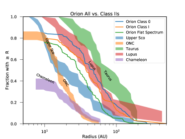
Figure 16: Cumulative distributions of disk radii within the Orion sample (lines) compared to Class II disk samples. The left panel shows the full sample, while the right panel only shows the non-multiple sample. The Orion protostellar disk radii are larger than those of Class II disks in most regions, comparable to Lupus, but smaller than Taurus. This, in addition to the radius comparison within Orion, suggests that there may not be a monotonoic growth of disks from the protostellar to Class II disk phase.

Appendix A Distance Estimates

Most protostars do not have a measurement of their parallax from Gaia DR2 due to their embedded nature, frequently resulting in $>$10 magnitudes of extinction at visual wavelengths and/or significant confusion due to scattered light. To estimate their distances, we rely on the nearby, more-evolved young stars that do have reliable parallax measurements. We use the input catalogs of McBride & Kounkel (2019) for Orion A, Kounkel et al. (2018) for Orion B, and Megeath et al. (2012) for L1622, selecting sources that have Gaia detection with $\sigma_{\pi}$ $<$ 0.2 mas. We multiplied the sample 10-fold through sampling the normal distribution of the parallaxes. We then used a fully connected neural network constructed in PyTorch with 1 hidden layer and 300 neurons to perform a 2-D extrapolation and predict the most likely parallax for the position of each protostar. To convert to distance from parallax, we use the conversion of d=1000/($\pi$+0.03) where $\pi$ is the parallax in milliarcseconds, correcting for the systematic offset from Lindegren et al. (2018). We assume a flat uncertainty in distance of 10 pc, based on the FWHM distribution of distances in a given population in the input sample.

We show the distribution of estimated distances throughout the clouds in Figure 17. The north-south distance gradient is obvious, but we also see that L1622 appears to be significantly closer than the rest of the locations within the Orion clouds. This is because L1622 is not part of Orion B, but rather one of the few remaining gaseous parts of Orion D. The distinction from Orion B can also be seen in the radial velocities toward these regions where they are discontinuous between L1622 and NGC 2068 in Orion B (Kounkel et al., 2018), but agree with Orion D. However, our sample contains only 9 protostars from this region (HOPS 1 through 7, HOPS-354, and HOPS-367), so its existence as a separate entity from Orion B will not significantly affect our results.

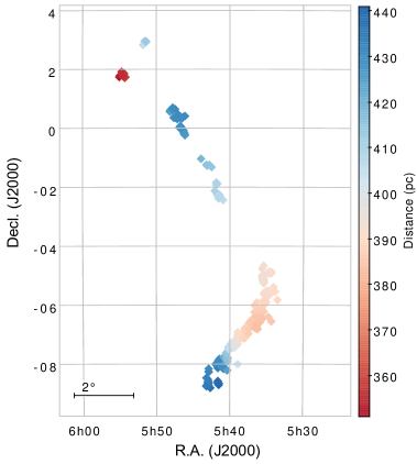
Figure 17: Plot of the estimated distance toward each protostar in the sample with the color scale denoting the estimated distance. There is clearly a gradient of increasing distance north and south of the Orion Nebula Cluster (Declination $\sim$5.5), and L1622 clearly stands out with a much closer estimated distance than the rest of the sample.

Appendix B Average Disk Dust Temperature

To determine the most appropriate dust temperature for estimating the dust disk masses from the 0.87 mm and 9 mm continuum emission, we used a grid of radiative transfer models to determine the average dust temperatures. The model grid sampled the parameter space given in Table 11. The use of this model grid enabled us to empirically derive an average dust temperature scaling based on the luminosity of a protostellar system and the radius of the disk. We were also able to investigate the variation of average dust temperature depending on dust disk mass. We used the Monte Carlo dust radiative transfer code RADMC-3D (Dullemond et al., 2012) to compute the temperature throughout the disk embedded within an envelope. The dust opacities in our model were parameterized by the maximum grain size (see Table 11) following the method outlined by Woitke et al. (2016).

Our models include a central protostar with an effective temperature of $T_{eff}=4000$ K and a luminosity, $L_{*}$, that is varied in our grid. It also includes a flared disk with a power-law density distribution,

$$\Sigma(R)=\Sigma_{0}\,\left(\frac{R}{1\,\text{au}}\right)^{-\gamma},$$ (B1)

$$\rho(R,z)=\frac{\Sigma(R)}{\sqrt{2\pi}\,h(R)}\,\exp\left[-\frac{1}{2}\left(\frac{z}{h(R)}\right)^{2}\right],$$ (B2)

$$h(R)=h_{0}\,\left(\frac{R}{1\,\text{au}}\right)^{\beta},$$ (B3)

with $R$ and $z$ defined for cylindrical coordinates. The disk is truncated at an inner radius of 0.1 au and an outer radius of $R_{disk}$, which is allowed to vary in our grid. The total dust disk mass, $M_{disk}$, and the surface density power law exponent, $\gamma$, are also allowed to vary, while the scale height at 1 au, $h_{0}$ is fixed at 0.1 au, and the scale height power-law exponent, $\beta$, is fixed at 1.15. The overall surface density profile normalized such that it has the disk mass desired.

We also also include an envelope in our model with the density distribution for a rotating collapsing cloud of material from Ulrich (1976),

$$\rho(r,\mu)=\frac{\dot{M}}{4\pi}\left(GM_{*}r^{3}\right)^{-\frac{1}{2}}\left(1+\frac{\mu}{\mu_{0}}\right)^{-\frac{1}{2}}\left(\frac{\mu}{\mu_{0}}+2\mu_{0}^{2}\frac{R_{c}}{r}\right)^{-1},$$ (B4)

where $\mu=\cos\theta$, and $r$ and $\theta$ are defined in the typical sense for spherical coordinates. We truncate the envelope at an inner radius of 0.1 au and an outer radius of 1500 au. Moreover, the centrifugal radius, $R_{c}$, where the envelope begins to flatten, is defined to be the same as the disk radius. Our envelope includes an outflow cavity with a half-opening angle of 45^∘ and a reduction of the density within the cavity of 50%. Note that the envelope density depends on the mass infall rate, while the total mass depends on that and the outer radius. If the density profile of the 0.001 M_☉ envelope is extended out to 5000 au, the envelope dust mass would instead be 0.037 M_☉ (total mass of 3.7 M_☉ assuming a gas-to-dust ratio of 100:1). Thus, the inner envelope density is fairly typical for Class 0 protostars in Orion (Furlan et al., 2016).

We calculated the average dust temperatures directly from the density grid for each RADMC-3D model using the equation

$$T_{dust,average}=\frac{\Sigma\,T_{i}\,m_{i}\,w_{i}}{\Sigma\,m_{i}\,w_{i}},$$ (B5)

where T_i is the temperature in each grid cell, m_i is the mass in each grid cell, and $\tau_{i}$ is the optical depth to each grid cell at 0.87 mm, computed from the z direction. The weighting function, $w_{i}$ is defined as

$$w_{i}=\frac{\pi}{2}\arctan[-4\pi\,\log_{10}(\tau_{i})-2\pi]+1.$$ (B6)

This weighting function asymptotes to constant values at both high and low values of $\tau_{i}$ such that regions of extremely high optical depth and extremely low optical depth are not given disproportionate weight in the average dust temperature.

Using these models, we found that a 1 L_☉ protostar has an average dust temperature of 43 K for a 50 au disk. We also confirmed that the average disk dust temperature scales $\propto$ L^0.25 considering the full set of disk radii (left panel, Figure 18). We further show in the middle panel of Figure 18 that the average dust temperature scales $\propto$R^-0.46, near the functional dependence expected from theory ($\propto$R^-0.5). It is also apparent that the average disk temperature is not quite linear in log-log space, and the temperature profile is flattening slightly for the largest radii. This is due to the backheating from the surrounding envelope. We did need to assume a dust disk mass of 33 M_⊕ to derive these relationships. However, we show that the average temperature for a disk with a radius of 50 au does not strongly depend on the mass of the disk in the right panel of Figure 18.

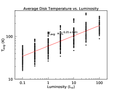
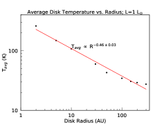
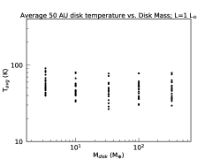
Figure 18: We show the average model disk temperatures as a function of luminosity (left), disk radius (middle), and dust disk mass (right). These relationships are used to determine our assumption of average disk temperature and how it should scale with disk radius and protostellar luminosity. In the left panel, we are including all dust disk masses to show that the dependence of the average disk temperature on luminosity does not strongly depend on dust disk mass. The middle panel only shows a single dust disk mass for clarity, but each point is the average dust temperature for a disk with a given radius. Lastly, the right panel shows the average dust temperature for disks with different masses, at a single luminosity of 1 L_☉. The spread at each dust disk mass is present because we plot all the disk radii for each mass.

Table 1: Model Grid Parameters

Parameter	Value
$L_{*}$ [L⊙]	0.1, 0.3, 1, 3, 10, 30, 100, 300
$M_{disk,dust}$ [M⊙]	$1\times 10^{-7}$, $3\times 10^{-7}$, $1\times 10^{-6}$, $3\times 10^{-6}$,$1\times 10^{-5}$, $3\times 10^{-5}$, $1\times 10^{-4}$, $3\times 10^{-4}$, 0.001,
$R_{disk}$ [au]	2, 5, 10, 30, 50, 100, 150, 200, 300
$\gamma$	1, 1.5
$M_{env,dust}$ [M⊙]	0.0001, 0.001
$a_{max}$ [$\mu$m]	1, $10^{3}$, $10^{4}$
$i$ [∘]	0, 30, 60, 90
$H.A.$ [hours]	-2.5, 0, 2.5

Note. — The parameters are described as follows: $L_{*}$ is the total luminosity of the protostar from the star and accretion, $M_{disk,dust}$ is the dust disk mass, $R_{disk}$ is the dust disk radius, $\gamma$ is the power-law of the surface density profile defined in Equation B1,$M_{env,dust}$ is the envelope dust mass, $a_{max}$ is the radius of the maximum dust grain size, $i$ is the inclination of the system, and $H.A.$ is the hour angle at which the observations were simulated.

Appendix C Images of all Protostars

We provide the images for the entire sample of Orion protostars in Figures 16 through 51 as image cutouts around each protostar. The cutout images are generally 1$\farcs$25 $\times$ 1$\farcs$25 except for the few sources that exceed this size (i.e., HOPS-136, HOPS-65). Figures 52 through 66 show larger images that encompass wide multiple systems. The images for each figure are available from the Harvard Dataverse (https://dataverse.harvard.edu) (Tobin, 2019a, b).

Appendix D Comparing Perseus Dust Disk Mass Methodologies to Orion

Here we analyze the differences in the dust disk mass distributions derived by Andersen et al. (2019) and Tychoniec et al. (2018) for the Perseus protostars. Andersen et al. (2019) used an independent method to calculate dust disk mass from lower resolution data, finding a strong correlation with the dust disk masses from Segura-Cox et al. (2018) and Tychoniec et al. (2018). Andersen et al. (2019) utilized Subcompact array data from the SMA with $\sim$4″ resolution, assumed that the flux density at 50 k$\lambda$ is dominated by the disk, and corrected for the estimated contribution of the envelope at this angular scale (see also Jørgensen et al., 2009). The masses calculated by Andersen et al. (2019) were consistent with those derived from the the 0$\farcs$2 resolution 9 mm data used by Tychoniec et al. (2018). However, Andersen et al. (2019) made different assumptions relative to this work and Tychoniec et al. (2018) for the calculation of dust temperatures; Andersen et al. (2019) adopted average dust temperatures of 30 K for the Class 0 protostars and 15 K for the Class I protostars, while Tychoniec et al. (2018) adopted 30 K for all protostars. We renormalized and scaled both the Tychoniec et al. (2018) and Andersen et al. (2019) dust disk masses to be consistent with our luminosity-dependent dust temperature method. We also corrected for the updated distance to Perseus of $\sim$300 pc. We plot the cumulative distributions for Class 0 and Class I protostars in Figure 19. Scaling the Tychoniec et al. (2018) data to account for the luminosity made little difference, but scaling the Andersen et al. (2019) results shifted the distributions to lower masses, but they are still not consistent with Orion. It is unclear if the difference in the mass distribution between Perseus and Orion results from a combination of methodology, using unresolved observations (Andersen et al., 2019), and/or wavelength (Tychoniec et al., 2018), and the additional uncertainty of the proper dust opacity at 8 mm.

To test if the dust opacity assumption at 9 mm is driving the discrepancy between Perseus and Orion, we compared the Orion VLA dust disk masses (Table 8) to the Perseus dust disk masses and show the result in Figure 20. The VLA 9 mm mass distributions for Orion are in much closer agreement with the Perseus distributions than the 0.87 mm mass distribution, but are still systematically shifted toward lower masses. The difference is less extreme for the Class I sample, and the difference in wavelength from 8.1 mm to 9 mm could contribute to the disagreement. A log rank test indicates that the probability of the Class 0 and Class I samples for Perseus and Orion to be drawn from the same sample is 1.6 $\times$ 10^-6 and 0.01, respectively. However, these masses for the Orion disks are upper limits because they do not have a free-free contribution removed, so the discrepancy could be larger.

We also compared the Orion 9 mm flux densities to the Perseus 9 mm flux densities (both normalized by distance squared) in Figure 21 to compare the samples without the conversion to dust mass. A log-rank test shows that the Class 0 flux densities at 9 mm for Perseus and Orion are consistent with being drawn from the same parent distribution with a probability of 0.12. The Perseus Class I and the Orion Class I + Flat Spectrum samples appear marginally inconsistent with being drawn from the same parent distribution with a probability of 0.01. It is also apparent that the distributions of masses for Class 0 and I protostars are shifted to higher masses for Perseus with respect to Orion, while the distributions of 9 mm flux densities are lower. This can be best explained by the higher luminosities of the Orion protostars resulting in lower masses due to the higher average dust temperatures. The flux densities compared here for both Perseus and Orion do not have correction for free-free emission, and since free-free emission is correlated with bolometric luminosity (e.g., Tychoniec et al., 2018), the higher luminosity protostars in Orion are likely to have higher overall 9 mm flux densities due to increased free-free emission.

Regardless of the results from the statistical comparison of the samples, we can see in Figure 20 that the VLA 9 mm mass distributions are shifted toward much higher masses than the ALMA 0.87 mm mass distributions. Thus, this is evidence that the dust opacity law at 9 mm is significantly different from the adopted opacities of Ossenkopf & Henning (1994) and extrapolated from 1.3 mm to 9 mm assuming a dust opacity spectral index of 1. The dust mass opacity at 9 mm would need to be as much as $\sim$7$\times$ larger to bring the 0.87 mm and 9 mm distributions into closer agreement.

From this analysis, it is clear that the Perseus dust disk masses at 8.1 mm may be significantly overestimated, and that further study of the Orion and Perseus populations at comparable wavelengths and spatial resolution is needed to determine if the mass distribution of Perseus is truly different from that of Orion. Moreover, additional investigation into the dust opacities at centimeter wavelengths is also needed to help reconcile the differences between observations of dust emission at very different wavelengths.

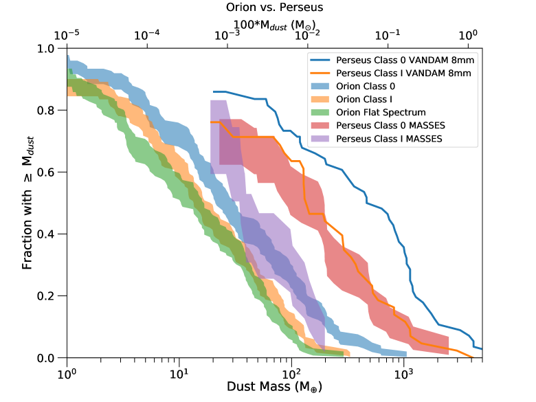
Figure 19: Cumulative distributions of dust disk masses within the full Orion sample relative to the protostellar dust disk mass measurements in Perseus from both VANDAM (Tychoniec et al., 2018) and MASSES (Andersen et al., 2019). The mass distributions from Tychoniec et al. (2018) are drawn as lines in this plot for clarity. This comparison enables us to explore differences that might be due to the wavelengths observed. The values from Andersen et al. (MASSES; 2019) indicate systematically lower masses than those in Tychoniec et al. (VANDAM; 2018), but are still not consistent with the mass distributions of the Orion sample.

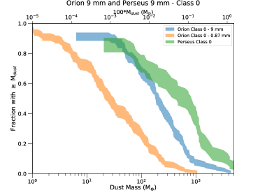
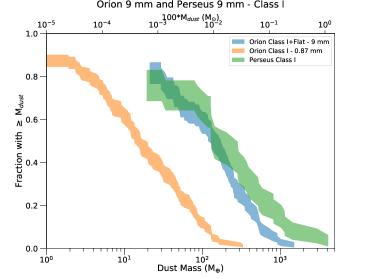
Figure 20: Cumulative distributions of dust disk masses within the Orion sample calculated from 9 mm data compared to the protostellar dust disk mass measurements in Perseus from VANDAM (Tychoniec et al., 2018). The dust disk masses from the Orion 0.87 mm data are also shown for comparison. The Class 0 sources are shown in the left panel and the Class I (combined with Flat Spectrum) in the right panel. Even without the free-free correction to the Orion data, the Class 0 sources from Perseus are still calculated to have higher masses. The Class I sources are more comparable, with some overlap in the distribution.

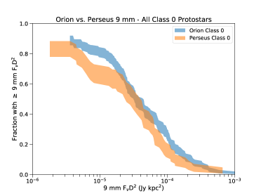
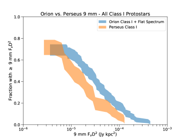
Figure 21: Cumulative distributions of 9 mm flux densities from the Orion and Perseus samples. The left panel shows Class 0 sources and the right panel shows the Class I sources. Given that the Perseus Class I sample includes both Class I and Flat Spectrum sources, we show both the distribution of 9 mm flux densities for the combined Class I and Flat Spectrum samples. The Orion Class 0 flux densities at 9 mm are statistically indistinguishable from the Perseus Class 0 flux densities at 9 mm, while the Class I flux densities at 9 mm from Orion compared to Perseus are marginally consistent, having a probability of 0.01 for being drawn from the same parent distribution.

Table 2: ALMA Observations

Fields	Date	Duration	Maximum Baseline	Antennas	PWV	Calibrators
		(min)	(m)		(mm)	Bandpass, Flux, Complex Gain
Orion B	2016 Sep 03	76	2483	36	0.39	J0522-3627, J0750+1231, J0552+0313
Orion B	2016 Sep 04	84	2483	41	0.79	J0510+1800, J0510+1800, J0552+0313
Orion A-1	2016 Sep 04	98	2483	41	0.73	J0510+1800, J0510+1800, J0541-0541
Orion A-1	2016 Sep 05	98	2483	41	0.53	J0510+1800, J0510+1800, J0541-0541
Orion A-2	2016 Sep 06	82	2483	39	0.42	J0510+1800, J0510+1800, J0541-0541
Orion A-2	2016 Sep 06	86	2483	34	0.43	J0510+1800, J0522-3627, J0541-0541
Orion A-1	2017 Jul 19	97	3697	41	0.47	J0510+1800, J0423-0120, J0541-0541
Orion A-2	2017 Jul 19	84	3697	42	0.42	J0510+1800, J0423-0120, J0541-0541
Orion B	2017 Jul 19	75	3697	41	0.58	J0510+1800, J0423-0120, J0552+0313

Note. — The Orion B fields include all HOPS protostars located at Declinations greater than -4.5. The Orion A fields include HOPS protostars below Dec. = -4.5°; fields denoted A-1 include protostars with numbers between 10 and 175, and fields denoted A-2 include HOPS protostars with numbers greater than 175.

Table 3: ALMA Fields

Field	RA	Dec.	Lbol	Tbol	Distance	Class	Sources
	(J2000)	(J2000)	(L☉)	(K)	(pc)
HH270VLA1	05:51:34.626	+02:56:45.02	7.0	32.0	430.1	0	2
HH270mms1	05:51:22.631	+02:56:06.73	8.3	72.0	405.7	I	2
HH270mms2	05:51:22.559	+02:55:42.78	4.7	249.0	413.3	Flat	1
HH111mms	05:51:46.238	+02:48:29.65	23.0	78.0	410.6	I	2
HOPS-367	05:54:36.259	+01:53:54.02	0.0	249.4	354.9	I	1
HOPS-7	05:54:20.045	+01:50:42.75	0.5	58.0	357.1	0	1
HOPS-6	05:54:18.411	+01:49:03.43	0.1	112.5	357.0	I	0
HOPS-5	05:54:32.163	+01:48:07.16	0.4	187.1	354.6	I	1
HOPS-4	05:54:53.765	+01:47:09.96	0.4	203.3	351.6	I	1
HOPS-354	05:54:24.253	+01:44:19.39	6.6	34.8	355.4	0	1
HOPS-3	05:54:56.966	+01:42:56.19	0.6	467.5	351.0	Flat	1
HOPS-2	05:54:09.129	+01:42:51.98	0.5	356.5	357.4	I	1
HOPS-1	05:54:12.336	+01:42:35.49	1.5	72.6	356.9	I	1
HOPS-346	05:47:42.986	+00:40:57.50	0.3	649.5	430.6	Flat	0
HOPS-345	05:47:38.976	+00:38:36.34	0.5	219.4	430.7	I	1
HOPS-406	05:47:43.362	+00:38:22.45	0.5	24.6	430.3	0	1
HOPS-406-d	05:47:43.360	+00:38:22.43	0.2	64.0	425.8	0	1
HOPS-344	05:47:24.724	+00:37:35.18	0.1	408.2	431.4	I	1
HOPS-343	05:47:59.029	+00:35:32.85	3.9	82.1	427.6	I	1
HOPS-342	05:47:57.088	+00:35:27.38	0.3	312.6	427.8	I	1
HOPS-404	05:48:07.761	+00:33:50.79	1.0	26.1	430.1	0	1
HOPS-341	05:47:00.994	+00:26:22.23	2.1	39.4	430.9	0	2
HOPS-340	05:47:01.291	+00:26:21.51	1.9	40.6	430.9	0	2
HOPS-338	05:46:57.343	+00:23:50.24	0.2	53.7	430.7	0	2
HOPS-337	05:46:55.101	+00:23:34.58	0.9	128.8	430.7	I	1
HOPS-336	05:46:02.280	+00:23:30.73	0.0	164.6	430.5	I	1
HOPS-393	05:46:42.482	+00:23:01.28	0.1	250.5	430.7	I	1
HOPS-335	05:47:05.860	+00:22:38.85	0.4	81.1	430.5	I	0
HOPS-366	05:47:03.981	+00:22:10.52	6.4	292.2	430.5	I	2
HOPS-361	05:47:04.776	+00:21:42.87	479.0	69.0	430.4	0	7
HOPS-392	05:46:16.482	+00:21:36.03	0.1	62.4	430.4	0	1
HOPS-334	05:46:48.524	+00:21:28.22	0.1	506.7	430.6	Flat	0
HOPS-347	05:47:15.894	+00:21:23.79	0.5	33.5	430.2	0	1
HOPS-365	05:47:10.615	+00:21:14.14	19.3	160.3	430.3	I	1
HOPS-359	05:47:24.807	+00:20:59.89	10.0	36.7	429.4	0	1
HOPS-333	05:47:22.884	+00:20:58.34	0.2	240.9	429.6	Flat	0
HOPS-391	05:47:17.060	+00:20:53.30	0.1	58.1	430.2	0	0
HOPS-390	05:47:32.442	+00:20:21.87	3.2	54.3	428.4	0	1
HOPS-364	05:47:36.574	+00:20:06.18	33.0	96.7	427.8	I	2
HOPS-331	05:46:28.320	+00:19:49.40	0.3	82.5	430.3	Flat	1
HOPS-407	05:46:28.244	+00:19:27.01	0.7	26.8	419.1	0	1
HOPS-329	05:47:01.607	+00:17:58.88	2.4	89.2	430.2	I	1
HOPS-326	05:46:39.584	+00:04:16.60	0.5	58.8	428.8	0	1
HOPS-325	05:46:39.253	+00:01:14.95	6.2	49.2	428.5	0	1
HOPS-363	05:46:43.117	+00:00:52.45	22.5	367.6	428.4	Flat	2
HOPS-324	05:46:37.543	+00:00:33.98	2.2	89.9	428.4	I	1
HOPS-389	05:46:47.024	+00:00:27.03	6.0	42.8	428.4	0	4
HOPS-323	05:46:47.688	+00:00:25.30	9.9	82.9	428.4	I	3
HOPS-322	05:46:46.492	+00:00:16.12	0.5	71.3	428.3	I	1
HOPS-321	05:46:33.166	+00:00:02.23	3.7	78.6	428.4	I	1
HOPS-403	05:46:27.746	-00:00:53.82	4.1	43.9	428.2	0	1
HOPS-373	05:46:30.685	-00:02:35.30	5.3	36.9	428.1	0	2
HOPS-320	05:46:14.206	-00:05:26.84	0.4	87.0	427.7	I	1
HOPS-388	05:46:13.129	-00:06:04.53	26.7	321.9	427.7	Flat	1
HOPS-319	05:46:12.999	-00:08:14.85	0.0	464.2	427.4	I	0
HOPS-318	05:46:13.502	-00:08:55.32	0.1	312.6	427.3	Flat	1
HOPS-387	05:46:07.842	-00:10:00.87	5.4	118.3	427.2	I	4
HOPS-386	05:46:08.498	-00:10:02.64	22.6	147.4	427.2	I	5
HOPS-317	05:46:08.591	-00:10:38.53	4.8	47.5	427.1	0	2
HOPS-402	05:46:09.973	-00:12:16.84	0.6	24.2	426.9	0	1
HOPS-401	05:46:07.652	-00:12:20.73	0.6	26.0	426.9	0	1
HOPS-316	05:46:07.291	-00:13:23.01	4.2	55.2	426.8	0	1
HOPS-358	05:46:07.231	-00:13:29.89	25.0	41.7	426.8	0	1
HOPS-385	05:46:04.773	-00:14:16.29	11.8	377.1	426.7	Flat	1
HOPS-315	05:46:03.631	-00:14:49.16	6.2	180.3	426.6	I	1
HH212mms	05:43:51.411	-01:02:53.17	14.0	53.0	413.2	0	1
HOPS-312	05:43:05.706	-01:15:54.28	0.7	46.7	416.3	0	2
HOPS-400	05:42:45.232	-01:16:14.19	2.9	35.0	415.4	0	2
HOPS-311	05:43:03.042	-01:16:28.92	2.8	383.0	416.1	Flat	1
HOPS-310	05:42:27.676	-01:20:00.99	13.8	51.8	414.3	0	1
HOPS-305	05:41:45.377	-01:51:56.77	1.0	300.7	409.6	Flat	1
HOPS-357	05:41:39.098	-01:52:07.46	15.0	628.2	409.4	Flat	2
HOPS-384	05:41:44.086	-01:54:45.10	1477.9	51.9	409.5	0	3
HOPS-304	05:41:45.942	-01:56:26.12	4.2	354.9	409.5	Flat	2
HOPS-303	05:42:02.619	-02:07:45.69	1.5	43.2	410.0	0	1
HOPS-299	05:41:44.584	-02:16:06.27	19.7	277.0	408.7	I	1
HOPS-300	05:41:24.211	-02:16:06.42	0.8	93.7	407.9	I	1
HOPS-298	05:41:37.174	-02:17:17.01	31.1	169.3	408.4	I	2
HOPS-297	05:41:23.272	-02:17:35.77	0.2	274.9	407.8	I	1
HOPS-399	05:41:24.936	-02:18:08.53	6.3	31.1	407.9	0	1
HOPS-372	05:41:26.342	-02:18:20.01	4.8	37.3	407.9	0	1
HOPS-398	05:41:29.399	-02:21:17.06	1.0	23.0	408.0	0	1
HOPS-295	05:41:28.944	-02:23:19.35	0.3	86.6	407.9	I	1
HOPS-294	05:40:51.714	-02:26:48.62	2.8	606.8	406.4	Flat	1
HOPS-107	05:35:23.340	-04:40:10.45	5.1	472.0	392.7	Flat	1
HOPS-105	05:35:32.285	-04:46:48.46	0.1	520.3	392.6	Flat	1
HOPS-102	05:34:35.180	-04:52:17.90	0.5	479.2	392.3	I	1
S13-021010	05:34:19.630	-04:53:23.54	0.2	64.0	392.0	None	0
HOPS-100	05:34:21.387	-04:55:14.80	0.0	605.1	392.0	I	0
HOPS-99	05:34:29.500	-04:55:30.61	1.3	48.9	392.1	0	1
HOPS-96	05:35:29.720	-04:58:48.79	6.2	35.6	392.7	0	1
HOPS-383	05:35:29.813	-04:59:51.14	7.8	45.8	392.8	0	1
HOPS-95	05:35:34.197	-04:59:52.22	0.8	41.8	392.8	0	1
HOPS-94	05:35:16.152	-05:00:02.26	6.6	123.0	392.7	I	0
HOPS-93	05:35:15.030	-05:00:08.20	0.4	107.3	392.7	I	1
HOPS-92	05:35:18.317	-05:00:32.97	20.1	186.3	392.7	Flat	3
HOPS-91	05:35:18.914	-05:00:50.86	4.1	41.7	392.7	0	1
HOPS-90	05:35:34.474	-05:00:52.02	2.8	417.7	392.8	Flat	1
HOPS-89	05:35:19.958	-05:01:02.56	1.6	158.3	392.7	Flat	1
HOPS-88	05:35:22.430	-05:01:14.15	15.8	42.4	392.7	0	1
HOPS-87	05:35:23.472	-05:01:28.70	36.5	38.1	392.7	0	2
HOPS-86	05:35:23.649	-05:01:40.26	3.3	112.7	392.7	I	3
HOPS-85	05:35:28.184	-05:03:40.93	16.3	174.2	392.8	Flat	2
HOPS-84	05:35:26.570	-05:03:55.11	49.1	90.8	392.8	I	2
HOPS-82	05:35:19.726	-05:04:54.58	2.4	116.4	392.7	Flat	1
HOPS-81	05:35:27.952	-05:04:58.15	1.2	40.1	392.8	0	1
HOPS-80	05:35:25.187	-05:05:09.45	0.1	275.3	392.8	Flat	1
HOPS-78	05:35:25.824	-05:05:43.65	8.9	38.1	392.8	0	4
HOPS-77	05:35:31.535	-05:05:47.25	12.9	550.3	392.8	Flat	3
HOPS-76	05:35:25.751	-05:05:57.94	1.9	135.5	392.8	I	2
HOPS-75	05:35:26.658	-05:06:10.29	4.0	67.9	392.8	0	2
HOPS-74	05:35:24.864	-05:06:21.38	1.1	516.5	392.8	Flat	1
HOPS-73	05:35:27.703	-05:07:03.50	1.7	43.0	392.8	0	1
HOPS-394	05:35:23.927	-05:07:53.47	6.6	45.5	392.8	0	1
HOPS-71	05:35:25.607	-05:07:57.32	5.6	277.5	392.8	I	4
HOPS-70	05:35:22.414	-05:08:04.81	6.9	619.3	392.8	Flat	4
HOPS-350	05:35:30.203	-05:08:18.85	0.6	57.3	392.8	I	0
HOPS-68	05:35:24.306	-05:08:30.58	5.7	100.6	392.8	I	1
HOPS-66	05:35:26.843	-05:09:24.58	21.0	264.9	392.8	Flat	2
HOPS-370	05:35:27.629	-05:09:33.47	360.9	71.5	392.8	I	2
HOPS-65	05:35:21.554	-05:09:38.70	0.4	545.7	392.8	I	1
HOPS-108	05:35:27.073	-05:10:00.37	38.3	38.5	392.8	0	5
HOPS-369	05:35:26.972	-05:10:17.14	35.3	379.2	392.8	Flat	3
HOPS-368	05:35:24.725	-05:10:30.21	68.9	137.5	392.8	I	1
HOPS-60	05:35:23.328	-05:12:03.06	21.9	54.1	392.8	0	1
HOPS-59	05:35:20.143	-05:13:15.52	49.4	528.4	392.8	Flat	2
HOPS-409	05:35:21.400	-05:13:17.50	8.2	28.4	392.8	0	1
HOPS-58	05:35:18.506	-05:13:38.20	4.5	620.0	392.8	Flat	1
HOPS-57	05:35:19.836	-05:15:08.53	3.2	421.2	392.8	Flat	2
HOPS-56	05:35:19.465	-05:15:32.72	23.3	48.1	392.8	0	5
HOPS-53	05:33:57.375	-05:23:30.40	26.4	45.9	390.5	0	1
HOPS-50	05:34:40.908	-05:31:44.39	4.2	51.4	391.5	0	1
HOPS-49	05:34:48.880	-05:31:45.94	0.7	356.8	391.8	I	1
HOPS-47	05:33:45.869	-05:32:58.09	0.1	558.4	389.8	Flat	1
HOPS-45	05:35:06.452	-05:33:35.10	8.5	517.8	391.9	Flat	2
HOPS-44	05:35:10.575	-05:35:06.32	1.7	43.8	391.8	0	1
HOPS-43	05:35:04.505	-05:35:14.35	3.3	75.0	391.7	I	1
HOPS-42	05:35:05.041	-05:35:40.70	0.3	200.9	391.7	I	1
HOPS-41	05:34:29.441	-05:35:42.68	1.9	82.3	390.9	I	1
HOPS-40	05:35:08.515	-05:35:59.38	2.7	38.1	391.6	0	1
HOPS-38	05:35:04.718	-05:37:12.28	0.2	58.5	391.4	0	0
HOPS-36	05:34:26.430	-05:37:40.51	1.0	374.6	390.6	Flat	1
HOPS-382	05:35:21.668	-05:37:57.86	0.1	204.4	391.4	I	0
HOPS-33	05:34:45.209	-05:39:56.80	0.1	777.6	390.8	Flat	0
HOPS-32	05:34:35.451	-05:39:59.11	2.0	58.9	390.6	0	2
HOPS-30	05:34:44.062	-05:41:25.87	3.8	81.2	390.6	I	1
HOPS-29	05:34:49.045	-05:41:42.17	1.9	148.2	390.6	I	1
HOPS-28	05:34:47.292	-05:41:55.86	0.5	46.3	390.6	0	2
HOPS-24	05:34:46.937	-05:44:50.96	0.1	288.9	390.2	I	0
HOPS-20	05:33:30.713	-05:50:41.02	1.2	94.8	389.1	I	1
HOPS-19	05:35:25.994	-05:51:22.86	0.2	101.6	389.3	Flat	0
HOPS-18	05:35:05.492	-05:51:54.39	1.4	71.8	389.2	I	1
HOPS-17	05:35:07.176	-05:52:05.91	0.3	341.3	389.1	I	1
HOPS-15	05:36:19.018	-05:55:25.46	0.2	342.0	388.6	Flat	1
HOPS-16	05:35:00.813	-05:55:25.68	0.7	361.0	388.6	Flat	1
HOPS-13	05:35:24.560	-05:55:33.42	1.1	383.6	388.7	Flat	1
HOPS-371	05:35:10.417	-05:55:40.90	0.6	31.6	388.6	0	1
HOPS-12	05:35:08.603	-05:55:54.26	7.3	42.0	388.6	0	3
S13-006006	05:35:11.470	-05:57:05.09	0.3	28.0	388.4	None	0
HOPS-11	05:35:13.409	-05:57:58.10	9.0	48.8	388.3	0	1
HOPS-10	05:35:09.006	-05:58:27.55	3.3	46.2	388.2	0	1
HOPS-192	05:36:32.449	-06:01:16.21	1.4	202.5	387.8	Flat	1
HOPS-193	05:36:30.270	-06:01:17.40	1.2	226.7	387.8	I	2
HOPS-200	05:35:33.212	-06:06:09.64	0.3	244.4	387.1	Flat	1
HOPS-194	05:35:52.000	-06:10:01.84	12.7	645.0	386.6	Flat	1
HOPS-191	05:36:17.262	-06:11:11.00	0.6	196.7	386.6	I	1
HOPS-198	05:35:22.176	-06:13:06.24	0.9	61.4	386.0	0	1
HOPS-185	05:36:36.982	-06:14:57.98	1.0	96.9	386.1	I	1
HOPS-182	05:36:18.833	-06:22:10.23	71.1	51.9	385.1	0	4
HOPS-181	05:36:19.502	-06:22:12.36	6.2	131.3	385.1	I	4
HOPS-183	05:36:17.859	-06:22:28.09	0.3	224.5	385.1	Flat	1
HOPS-178	05:36:24.607	-06:22:41.30	20.0	155.1	385.1	I	1
HOPS-187	05:35:50.938	-06:22:43.49	0.3	1210.9	384.8	Flat	0
HOPS-179	05:36:21.840	-06:23:29.83	1.8	467.5	385.0	Flat	1
HOPS-176	05:36:23.582	-06:24:51.55	1.5	312.2	384.9	Flat	1
HOPS-175	05:36:24.061	-06:24:54.93	0.3	104.3	384.9	I	1
HOPS-174	05:36:25.855	-06:24:58.71	2.0	350.3	384.9	Flat	3
HOPS-380	05:36:25.297	-06:25:02.64	0.6	36.6	384.9	0	3
HOPS-173	05:36:26.037	-06:25:05.19	0.9	60.2	384.9	0	3
HOPS-199	05:34:39.865	-06:25:14.16	0.2	576.7	385.3	Flat	1
HOPS-186	05:35:47.278	-06:26:14.74	0.5	72.3	384.3	I	1
HOPS-189	05:35:30.893	-06:26:32.09	1.2	133.1	384.3	I	1
HOPS-188	05:35:29.820	-06:26:58.16	18.8	103.3	384.2	I	1
HOPS-190	05:35:28.496	-06:27:01.80	0.4	385.3	384.2	I	0
HOPS-172	05:36:19.442	-06:29:06.79	0.7	149.8	384.4	I	1
HOPS-379	05:37:07.710	-06:31:57.61	0.0	114.2	385.3	I	0
HOPS-170	05:36:41.331	-06:34:00.08	2.5	832.5	384.2	Flat	2
HOPS-197	05:34:15.882	-06:34:32.70	0.2	506.6	385.1	Flat	1
HOPS-177	05:35:50.016	-06:34:53.40	0.4	84.7	383.6	I	1
HOPS-163	05:37:17.280	-06:36:18.18	0.9	432.3	385.7	I	2
HOPS-164	05:37:00.454	-06:37:10.48	0.6	50.0	385.0	0	1
HOPS-171	05:36:17.198	-06:38:01.60	1.9	61.8	383.4	0	1
HOPS-169	05:36:36.122	-06:38:51.90	3.9	32.5	384.0	0	1
HOPS-166	05:36:25.126	-06:44:41.81	15.5	457.1	383.5	Flat	1
HOPS-168	05:36:18.934	-06:45:22.71	48.1	54.0	383.3	0	2
HOPS-167	05:36:19.794	-06:46:00.87	0.2	568.6	383.3	Flat	1
HOPS-203	05:36:22.839	-06:46:06.20	20.4	43.7	383.5	0	3
HOPS-165	05:36:23.541	-06:46:14.55	3.4	96.1	383.5	I	2
HOPS-378	05:36:25.644	-06:47:16.40	0.3	170.4	383.6	I	0
HOPS-159	05:37:53.736	-06:47:16.94	0.4	498.4	387.4	Flat	1
HOPS-160	05:37:51.041	-06:47:20.40	1.4	80.4	387.3	I	1
S13-038002	05:36:11.110	-06:49:11.29	0.1	40.0	383.0	None	0
HOPS-355	05:37:17.081	-06:49:49.33	1.2	44.9	385.8	0	1
HOPS-147	05:38:55.002	-06:56:18.63	0.1	619.6	390.6	Flat	0
HOPS-157	05:37:56.565	-06:56:39.19	3.8	77.6	387.7	I	1
HOPS-156	05:38:03.404	-06:58:15.81	0.3	90.1	388.1	I	1
HOPS-149	05:38:40.479	-06:58:21.68	11.5	484.6	389.9	Flat	2
HOPS-158	05:37:24.459	-06:58:32.77	2.7	591.6	386.2	Flat	2
HOPS-154	05:38:20.093	-06:59:04.84	0.1	166.7	388.9	I	1
HOPS-148	05:38:39.514	-06:59:30.33	0.4	262.9	389.9	I	1
HOPS-142	05:38:47.766	-07:00:26.89	0.0	231.8	390.3	I	0
HOPS-143	05:38:46.185	-07:00:48.56	4.3	242.1	390.3	I	1
HOPS-141	05:38:48.013	-07:00:49.46	0.2	741.6	390.4	Flat	0
HOPS-144	05:38:45.013	-07:01:01.74	2.2	99.2	390.2	I	2
HOPS-377	05:38:45.540	-07:01:02.17	3.8	53.7	390.2	0	2
HOPS-145	05:38:43.838	-07:01:13.22	2.1	133.7	390.2	I	2
HOPS-139	05:38:49.617	-07:01:17.79	2.9	84.3	390.5	I	1
HOPS-140	05:38:46.281	-07:01:53.47	0.6	137.2	390.3	I	3
HOPS-376	05:38:18.149	-07:02:26.26	217.9	492.0	388.8	Flat	1
HOPS-137	05:38:53.951	-07:02:33.21	0.2	43.7	390.9	0	0
HOPS-138	05:38:48.327	-07:02:43.44	0.1	42.8	390.5	0	2
HOPS-136	05:38:46.537	-07:05:37.46	0.7	161.7	390.6	I	1
HOPS-153	05:37:57.011	-07:06:56.48	4.4	39.4	387.9	0	1
HOPS-152	05:37:58.757	-07:07:25.32	0.7	53.8	388.0	0	1
HOPS-150	05:38:07.525	-07:08:29.22	3.8	245.2	388.5	Flat	2
HOPS-129	05:39:11.847	-07:10:35.00	1.7	191.3	393.8	Flat	1
HOPS-133	05:39:05.833	-07:10:39.39	3.3	74.6	393.1	I	1
HOPS-131	05:39:07.571	-07:10:52.10	0.2	82.3	393.4	I	1
HOPS-135	05:38:45.315	-07:10:55.92	1.1	130.3	391.1	I	1
HOPS-132	05:39:05.360	-07:11:05.24	1.7	616.3	393.2	Flat	1
HOPS-134	05:38:42.781	-07:12:43.84	7.8	781.9	391.2	Flat	1
HOPS-130	05:39:02.960	-07:12:52.27	1.5	156.7	393.2	I	1
HOPS-396	05:39:13.146	-07:13:11.71	0.0	58.7	394.5	0	0
HOPS-122	05:39:45.127	-07:19:13.51	0.0	246.0	400.1	I	1
HOPS-127	05:39:00.941	-07:20:22.59	0.4	133.3	394.5	I	1
HOPS-375	05:39:18.360	-07:20:23.56	0.0	695.2	396.5	I	0
HOPS-128	05:38:52.008	-07:21:06.04	0.8	469.2	393.6	Flat	2
HOPS-123	05:39:33.299	-07:22:57.35	0.4	50.1	399.0	0	1
HOPS-121	05:39:33.703	-07:23:02.00	0.3	34.8	399.1	0	1
HOPS-119	05:39:50.649	-07:23:30.44	1.1	573.8	402.3	Flat	1
HOPS-408	05:39:30.748	-07:23:59.38	0.5	37.9	398.9	0	1
HOPS-408-d	05:39:30.750	-07:23:59.40	0.5	38.0	398.9	0	1
HOPS-118	05:39:54.584	-07:24:14.83	0.3	552.8	403.4	Flat	1
HOPS-117	05:39:55.440	-07:24:19.47	0.1	277.0	403.6	Flat	1
HOPS-395-d	05:39:17.000	-07:24:26.64	0.5	32.0	397.2	0	2
HOPS-395	05:39:16.998	-07:24:26.64	0.5	31.7	397.2	0	2
HOPS-116	05:39:57.895	-07:25:13.11	0.3	411.1	404.4	Flat	1
HOPS-114	05:40:01.373	-07:25:38.64	0.0	117.3	405.3	I	1
HOPS-115	05:39:56.503	-07:25:51.52	0.3	461.3	404.2	Flat	1
HOPS-124	05:39:19.983	-07:26:11.18	58.3	44.8	398.0	0	2
HOPS-120	05:39:34.315	-07:26:11.43	0.3	455.3	400.0	Flat	1
HOPS-125	05:39:19.613	-07:26:18.81	9.6	110.5	398.0	Flat	2
HOPS-287	05:40:08.782	-07:27:27.68	0.8	117.8	407.6	I	1
HOPS-291	05:39:57.967	-07:28:57.53	0.1	340.1	405.5	Flat	1
HOPS-285	05:40:05.901	-07:29:32.89	0.1	66.5	407.5	0	0
HOPS-290	05:39:57.412	-07:29:33.39	1.8	47.3	405.5	0	2
HOPS-288	05:39:55.945	-07:30:27.97	135.5	48.6	405.5	0	2
HOPS-286	05:39:58.700	-07:31:12.10	0.6	123.7	406.3	I	0
HOPS-282	05:40:26.089	-07:37:32.01	0.8	95.1	414.7	I	2
HOPS-281	05:40:24.619	-07:43:08.25	1.3	189.3	416.1	Flat	2
HOPS-276	05:40:42.913	-07:45:01.90	0.2	303.8	421.0	I	1
HOPS-279	05:40:17.790	-07:48:25.99	6.0	382.0	416.1	Flat	1
HOPS-280	05:40:14.932	-07:48:48.70	3.3	121.2	415.5	I	1
HOPS-275	05:40:36.347	-07:49:06.99	0.1	146.4	420.7	I	1
HOPS-271	05:40:43.964	-07:49:30.43	0.1	108.4	422.4	I	0
HOPS-267	05:41:19.661	-07:50:41.02	1.1	186.2	428.9	I	1
HOPS-278	05:40:20.350	-07:51:14.93	0.2	96.3	417.6	I	1
HOPS-265	05:41:20.322	-07:53:10.64	0.1	635.1	429.5	Flat	1
HOPS-266	05:41:11.811	-07:53:35.80	0.0	190.7	428.5	Flat	0
HOPS-262	05:41:23.966	-07:53:41.96	0.9	202.4	430.0	Flat	2
HOPS-263	05:41:23.683	-07:53:46.75	0.7	145.1	430.0	I	2
HOPS-253	05:41:28.769	-07:53:51.00	0.6	321.1	430.6	Flat	1
HOPS-258	05:41:24.711	-07:54:08.46	1.1	385.7	430.2	Flat	1
HOPS-270	05:40:40.534	-07:54:39.81	0.3	96.6	423.1	I	1
HOPS-274	05:40:20.716	-07:54:59.72	1.9	546.5	418.9	Flat	2
HOPS-254	05:41:24.515	-07:55:07.28	5.9	114.7	430.4	I	1
HOPS-374	05:41:25.459	-07:55:18.94	0.2	56.9	430.5	0	1
HOPS-261	05:41:18.885	-07:55:29.06	2.3	149.5	429.8	I	2
HOPS-257	05:41:19.873	-07:55:46.59	0.3	292.6	430.0	Flat	1
HOPS-273	05:40:20.877	-07:56:24.71	2.2	243.3	419.4	I	1
HOPS-247	05:41:26.222	-07:56:51.61	3.1	42.8	430.9	0	1
HOPS-248	05:41:22.093	-07:58:03.00	2.1	484.3	430.7	Flat	2
HOPS-245	05:41:22.860	-07:58:55.95	0.3	302.1	431.0	Flat	1
HOPS-264	05:40:59.106	-08:00:14.29	0.1	402.3	428.3	Flat	1
HOPS-268	05:40:38.328	-08:00:36.00	1.1	113.9	424.3	I	1
HOPS-239	05:41:27.059	-08:00:54.75	0.2	116.2	431.8	I	1
HOPS-241	05:41:26.398	-08:01:02.13	0.7	100.3	431.8	I	1
HOPS-240	05:41:25.967	-08:01:15.85	0.1	191.0	431.8	I	1
HOPS-233	05:41:52.309	-08:01:21.97	0.0	106.2	432.6	I	0
HOPS-234	05:41:49.949	-08:01:26.50	2.3	79.8	432.7	I	1
HOPS-284	05:38:51.483	-08:01:27.44	0.7	913.9	403.4	Flat	1
HOPS-238	05:41:26.639	-08:03:12.60	0.4	269.1	432.2	I	1
HOPS-237	05:41:28.973	-08:03:25.84	0.3	177.7	432.5	I	1
HOPS-236	05:41:30.207	-08:03:41.54	4.9	332.8	432.6	Flat	1
HOPS-251	05:40:54.013	-08:05:13.02	0.6	345.7	428.7	Flat	1
HOPS-405	05:40:58.466	-08:05:36.09	1.6	35.0	429.3	0	1
HOPS-255	05:40:50.567	-08:05:48.69	0.6	572.0	428.4	Flat	2
HOPS-249	05:40:52.857	-08:05:48.76	0.1	268.5	428.7	Flat	1
HOPS-235	05:41:25.344	-08:05:54.81	4.8	680.1	432.6	Flat	1
HOPS-244	05:41:01.993	-08:06:01.87	1.4	127.3	429.9	I	1
HOPS-252	05:40:49.920	-08:06:08.27	1.8	329.2	428.5	Flat	1
HOPS-256	05:40:45.256	-08:06:42.15	0.1	72.4	427.7	0	1
HOPS-243	05:41:01.662	-08:06:44.78	0.4	50.8	430.0	0	1
HOPS-250	05:40:48.842	-08:06:57.24	6.8	69.4	428.5	0	1
HOPS-232	05:41:35.445	-08:08:22.48	1.1	187.9	434.0	I	1
HOPS-246	05:40:47.117	-08:09:47.80	0.4	95.6	429.1	I	1
HOPS-229	05:42:47.366	-08:10:08.75	0.3	471.6	431.0	Flat	0
HOPS-242	05:40:48.516	-08:11:08.95	0.6	836.7	429.6	Flat	2
HOPS-259	05:40:20.877	-08:13:55.20	0.8	410.3	425.3	Flat	2
HOPS-260	05:40:19.392	-08:14:16.36	1.7	600.1	425.1	Flat	1
HOPS-397	05:42:48.875	-08:16:10.70	1.7	46.1	431.7	0	1
HOPS-223	05:42:48.461	-08:16:34.46	19.3	247.5	431.8	I	1
HOPS-221	05:42:47.053	-08:17:06.97	8.4	172.3	432.0	I	1
HOPS-215	05:43:09.584	-08:29:27.13	0.5	195.5	432.5	I	1
HOPS-216	05:42:55.535	-08:32:48.26	0.7	117.7	433.8	I	1
HOPS-228	05:41:34.171	-08:35:27.70	11.0	293.0	439.2	I	1
HOPS-214	05:42:47.225	-08:36:36.57	0.1	360.8	435.0	Flat	1
HOPS-211	05:42:58.357	-08:37:43.46	0.2	87.9	434.5	Flat	1
HOPS-227	05:41:32.331	-08:37:55.52	0.3	371.0	439.8	Flat	1
HOPS-210	05:42:58.270	-08:38:05.39	1.3	204.9	434.6	Flat	1
HOPS-213	05:42:48.094	-08:40:08.29	1.5	534.9	435.6	Flat	2
HOPS-226	05:41:30.060	-08:40:09.40	0.9	350.2	440.4	Flat	1
HOPS-224	05:41:32.025	-08:40:09.73	3.0	48.6	440.3	0	1
HOPS-225	05:41:30.347	-08:40:17.57	0.8	432.5	440.5	Flat	1
HOPS-209	05:42:52.888	-08:41:41.17	0.3	554.1	435.6	I	0
HOPS-220	05:41:29.778	-08:42:46.00	0.3	193.6	441.0	I	1
HOPS-219	05:41:29.250	-08:43:04.25	2.0	90.0	441.1	I	1
HOPS-208	05:42:52.717	-08:44:12.69	0.0	373.5	436.1	Flat	1
HOPS-206	05:43:07.260	-08:44:31.09	2.3	65.1	435.2	0	1
HOPS-204	05:43:10.183	-08:46:07.89	1.3	85.4	435.4	I	1
HOPS-207	05:42:38.578	-08:50:18.56	0.5	446.2	438.5	Flat	0

Note. — The fields HOPS-395, HOPS-406, and HOPS-408 were observed twice due to a different target name being assigned to the same position. The duplicate fields have a ‘-d’ appended to their field name. The field names that begin with S13 are taken from Stutz et al. (2013), which identified them as potential protostellar sources. However, no sources were detected within the S13 fields.

Table 4: VLA Observations

Note. — The standard observation length was 2.5 hours, and we achieved $\sim$1 hour on-source. For the observations with Number of sources listed as 2, the observation length was 4 hours, and we were able to still reach $\sim$1 hr on source for each source in the SB. Observing efficiency is improved due to sharing the flux and bandpass calibration in addition to the fixed 10 minute overhead at the start of the observation.

Table 5: VLA Fields

Table 6: Targeted Field Detection Summary

Sample	ALMA 0.87 mm	ALMA 0.87 mm	VLA 9 mm	VLA 9 mm
	Targeted	Detected	Targeted	Detected
Class 0	94	86 (125)	88	76 (122)
Class I	128	109 (130)	10	10 (43)
Flat Spectrum	103	91 (118)	$\cdots$	$\cdots$ (26)
OMC1N	$\cdots$	$\cdots$ ( $\cdots$ )	4	4 (16)
Other	3	0	$\cdots$	$\cdots$ (25)
Total	328	286 (379)	102	90 (232)

Note. — The numbers listed refer whether or not a source was detected in apparent association with the HOPS protostar targeted. The numbers in parentheses refer to the number of continuum sources detected toward protostars in a given category. For OMC1N, we only targeted this region with 4 VLA fields and detected sources in all 4 fields. See Section 3.1 for further details on the detection statistics.

Table 10: Disk Masses and Radii Distribution Properties

Sample	Mean $M_{dust}$	$\sigma$(log10$\left(\frac{M_{dust}}{M_{\earth}}\right)$)	Median $M_{dust}$	Mean RDisk	$\sigma$(log10$\left(\frac{R_{disk}}{1~{}AU}\right)$)	Median $R_{disk}$	Ref.
	($M_{\earth}$)		(M⊕)	(AU)		(AU)
All Sources (including multiples)
Class 0	25.9${}^{+7.7}_{-4.0}$	0.80${}^{+0.003}_{-0.010}$	25.7${}^{+102.9}_{-6.7}$	44.9${}^{+5.8}_{-3.4}$	0.38${}^{+0.002}_{-0.004}$	48.1${}^{+79.6}_{-24.5}$	1
Class I	14.9${}^{+3.8}_{-2.2}$	0.76${}^{+0.008}_{-0.019}$	15.6${}^{+49.5}_{-4.9}$	37.0${}^{+4.9}_{-3.0}$	0.42${}^{+0.001}_{-0.005}$	38.1${}^{+64.0}_{-17.5}$	1
Flat Spectrum	11.6${}^{+3.5}_{-1.9}$	0.81${}^{+0.011}_{-0.016}$	13.8${}^{+43.8}_{-3.3}$	28.5${}^{+3.7}_{-2.3}$	0.38${}^{+0.001}_{-0.007}$	30.9${}^{+51.3}_{-13.0}$	1
Orion Class 0 (T = 20K, $\kappa$=3.45)	111.6${}^{+36.5}_{-19.0}$	0.87${}^{+0.010}_{-0.017}$	116.7${}^{+420.8}_{-30.3}$				1
Orion Class I (T = 20K, $\kappa$=3.45)	42.1${}^{+13.2}_{-7.4}$	0.91${}^{+0.017}_{-0.029}$	48.5${}^{+164.4}_{-10.8}$				1
Orion Flat Spectrum (T = 20K, $\kappa$=3.45)	34.3${}^{+11.1}_{-5.9}$	0.87${}^{+0.007}_{-0.017}$	40.8${}^{+124.9}_{-9.8}$				1
Northern ISF	14.5${}^{+6.1}_{-2.6}$	0.77${}^{+0.001}_{-0.013}$	14.7${}^{+58.4}_{-5.0}$	36.3${}^{+7.5}_{-3.6}$	0.41${}^{+0.001}_{-0.009}$	38.4${}^{+63.1}_{-18.0}$	1
L1641 and Southern ISF	13.9${}^{+2.9}_{-1.9}$	0.82${}^{+0.009}_{-0.016}$	15.2${}^{+49.6}_{-3.6}$	39.6${}^{+3.5}_{-2.3}$	0.34${}^{+0.001}_{-0.002}$	39.7${}^{+62.9}_{-24.6}$	1
Orion B	22.8${}^{+7.2}_{-3.6}$	0.77${}^{+0.006}_{-0.014}$	24.3${}^{+78.7}_{-6.5}$	44.6${}^{+6.3}_{-3.4}$	0.36${}^{+0.004}_{-0.002}$	45.6${}^{+74.7}_{-25.5}$	1
Non-multiple Sources
Class 0	38.1${}^{+18.9}_{-8.4}$	0.83${}^{+0.047}_{-0.058}$	52.5${}^{+133.5}_{-13.1}$	53.7${}^{+8.4}_{-4.2}$	0.30${}^{+0.002}_{-0.009}$	55.0${}^{+84.1}_{-34.5}$	1
Class I	13.4${}^{+4.6}_{-2.4}$	0.83${}^{+0.014}_{-0.033}$	15.2${}^{+49.5}_{-4.4}$	35.4${}^{+6.1}_{-3.5}$	0.44${}^{+0.002}_{-0.011}$	38.0${}^{+63.8}_{-12.5}$	1
Flat Spectrum	14.3${}^{+6.5}_{-3.0}$	0.85${}^{+0.029}_{-0.040}$	22.0${}^{+53.2}_{-3.5}$	36.0${}^{+5.9}_{-3.2}$	0.35${}^{+0.007}_{-0.014}$	38.3${}^{+61.3}_{-19.1}$	1
Orion Class 0 (T = 20K, $\kappa$=3.45)	126.0${}^{+74.1}_{-32.3}$	0.95${}^{+0.070}_{-0.081}$	187.4${}^{+540.2}_{-32.7}$				1
Orion Class I (T = 20K, $\kappa$=3.45)	31.1${}^{+13.2}_{-6.7}$	0.99${}^{+0.019}_{-0.041}$	33.1${}^{+140.1}_{-9.0}$				1
Orion Flat Spectrum (T = 20K, $\kappa$=3.45)	33.1${}^{+17.2}_{-7.6}$	0.96${}^{+0.023}_{-0.043}$	43.5${}^{+129.3}_{-9.5}$				1
Northern ISF	22.7${}^{+13.1}_{-4.5}$	0.68${}^{+0.015}_{-0.041}$	23.7${}^{+68.5}_{-9.3}$	44.5${}^{+11.9}_{-3.9}$	0.31${}^{+0.025}_{-0.000}$	40.9${}^{+70.2}_{-32.0}$	1
L1641 and Southern ISF	15.3${}^{+4.5}_{-2.7}$	0.91${}^{+0.022}_{-0.034}$	18.7${}^{+67.0}_{-3.8}$	47.7${}^{+5.0}_{-3.0}$	0.31${}^{+0.001}_{-0.003}$	48.2${}^{+76.9}_{-32.0}$	1
Orion B	17.9${}^{+10.8}_{-4.2}$	0.94${}^{+0.012}_{-0.033}$	28.3${}^{+73.8}_{-4.7}$	49.0${}^{+8.1}_{-3.8}$	0.28${}^{+0.000}_{-0.011}$	54.5${}^{+72.9}_{-34.7}$	1
Oph Class I	3.83${}^{+1.62}_{-1.31}$	0.86${}^{+0.06}_{-0.02}$	4.2${}^{+17.7}_{-0.6}$				2
Oph Flat Spectrum	2.49${}^{+0.82}_{-0.82}$	0.83${}^{+0.03}_{-0.01}$	2.8${}^{+8.2}_{-0.7}$				2
Taurus	27.6${}^{+72.7}_{-2.3}$	0.91${}^{+0.095}_{-0.092}$	45.0${}^{+92.4}_{-15.7}$				3
Perseus Class 0	376.5${}^{+220.3}_{-89.5}$	0.86${}^{+0.042}_{-0.059}$	549.8${}^{+1149.0}_{-108.4}$				1,4
Perseus Class I	142.6${}^{+93.0}_{-38.9}$	0.83${}^{+0.015}_{-0.091}$	143.8${}^{+486.3}_{-73.5}$				1,4
Class II Disk Samples
Chameleon	1.6${}^{+0.9}_{-0.4}$	1.14${}^{+0.013}_{-0.042}$	1.8${}^{+9.1}_{-0.3}$				5
Lupus	5.08${}^{+1.78}_{-1.41}$	0.82${}^{+0.01}_{-0.01}$	3.5${}^{+15.2}_{-0.8}$				6
Taurus	3.3${}^{+1.0}_{-0.6}$	0.90${}^{+0.006}_{-0.020}$	4.9${}^{+11.7}_{-2.1}$				7
Oph	0.78${}^{+0.12}_{-0.11}$	0.97${}^{+0.06}_{-0.05}$	0.9${}^{+3.0}_{-0.2}$				2
Orion Nebula Cluster	0.7${}^{+0.3}_{-0.1}$	0.94${}^{+0.039}_{-0.033}$	1.9${}^{+7.0}_{-1.0}$				8
Upper Scorpius	0.36${}^{+0.1}_{-0.09}$	0.88${}^{+0.08}_{-0.05}$	0.2${}^{+1.0}_{-0.1}$				9

Note. — The mean disk masses and standard deviation of the log-normal distribution is derived from fitting the cumulative distribution function derived from the survival analysis with a Gaussian cumulative distribution function. The median disk dust masses include non-detections, while the median radii do not include non-detections. The sub- and superscripts on the median values correspond to the first and third quartiles of the distributions and are absolute values, not relative to the median. Multiple sources refer to any system with a companion detected with the VLA or ALMA within 10000 AU. References: This work (1), Williams et al. (2019) (2), Sheehan & Eisner (2017a) (3), Tychoniec et al. (2018) (4), Pascucci et al. (2016) (5), Ansdell et al. (2016) (6), Tripathi et al. (2017) (7), Eisner et al. (2018) (8), and Barenfeld et al. (2016) (9).

Table 11: Disk Mass and Radius Sample comparison

Sample	Disk Mass	Number	Disk Radius	Number
	Probability	Srcs	Probability	Srcs
All Sources (including multiples)
Class 0 vs. Class I	0.0014 (0.017)	133, 150 (125, 113)	0.63 (0.59)	131, 147 (104, 112)
Class 0 vs. Flat Spectrum	0.000014 (0.00045)	133, 132 (125, 111)	0.0002 (0.00054)	131, 129 (104, 88)
Class I vs. Flat Spectrum	0.061 (0.045)	150, 132 (113, 111)	0.003 (0.0089)	147, 129 (112, 88)
Northern ISF vs. L1641 and Southern ISF	0.71	76, 235	0.78	72, 203
Northern ISF vs. Orion B	0.062	76, 113	0.54	72, 105
Orion B vs. L1641 and Southern ISF	0.021	113, 235	0.24	105, 203
Non-multiple Sources
Class 0 vs. Class I	0.00001 (0.00019)	69, 110 (61, 91)	0.59 (0.16)	67, 108 (65, 89)
Class 0 vs. Flat Spectrum	0.00002 (0.00039)	69, 79 (61, 67)	0.04 (0.0094)	67, 78 (65, 65)
Class I vs. Flat Spectrum	0.73 (0.75)	110, 79 (91, 67)	0.13 (0.41)	108, 78 (89, 65)
Northern ISF vs. L1641 and Southern ISF	0.78	39, 165	0.89	36, 135
Northern ISF vs. Orion B	0.89	69, 63	0.66	36, 55
Orion B vs. L1641 and Southern ISF	0.30	63, 165	0.75	55, 135

Note. — The values in parentheses represent the probability values from the Anderson-Darling test that was used as an additional check on the robustness of the log-rank test for the cases where distributions may have crossed, limiting the effectiveness of the log-rank test. The only case where the Anderson-Darling test and the log-rank test differ significantly is Class 0 vs. Flat Spectrum for non-multiple sources.

References

- Allen et al. (2003) Allen, A., Li, Z., & Shu, F. H. 2003, ApJ, 599, 363, doi: 10.1086/379243
- Allen et al. (2008) Allen, T. S., Pipher, J. L., Gutermuth, R. A., et al. 2008, ApJ, 675, 491, doi: 10.1086/525241
- Alves et al. (2018) Alves, F. O., Girart, J. M., Padovani, M., et al. 2018, A&A, 616, A56, doi: 10.1051/0004-6361/201832935
- Andersen et al. (2019) Andersen, B. C., Stephens, I. W., Dunham, M. M., et al. 2019, ApJ, 873, 54, doi: 10.3847/1538-4357/ab05c7
- André et al. (1993) André, P., Ward-Thompson, D., & Barsony, M. 1993, ApJ, 406, 122, doi: 10.1086/172425
- Andrews et al. (2013) Andrews, S. M., Rosenfeld, K. A., Kraus, A. L., & Wilner, D. J. 2013, ApJ, 771, 129, doi: 10.1088/0004-637X/771/2/129
- Andrews et al. (2009) Andrews, S. M., Wilner, D. J., Hughes, A. M., Qi, C., & Dullemond, C. P. 2009, ApJ, 700, 1502, doi: 10.1088/0004-637X/700/2/1502
- Andrews et al. (2018) Andrews, S. M., Huang, J., Pérez, L. M., et al. 2018, ApJ, 869, L41, doi: 10.3847/2041-8213/aaf741
- Anglada et al. (1998) Anglada, G., Villuendas, E., Estalella, R., et al. 1998, AJ, 116, 2953, doi: 10.1086/300637
- Ansdell et al. (2016) Ansdell, M., Williams, J. P., van der Marel, N., et al. 2016, ApJ, 828, 46, doi: 10.3847/0004-637X/828/1/46
- Ansdell et al. (2018) Ansdell, M., Williams, J. P., Trapman, L., et al. 2018, ApJ, 859, 21, doi: 10.3847/1538-4357/aab890
- Aso et al. (2015) Aso, Y., Ohashi, N., Saigo, K., et al. 2015, ApJ, 812, 27, doi: 10.1088/0004-637X/812/1/27
- Aso et al. (2017) Aso, Y., Ohashi, N., Aikawa, Y., et al. 2017, ArXiv e-prints. https://arxiv.org/abs/1707.08697
- Astropy Collaboration et al. (2018) Astropy Collaboration, Price-Whelan, A. M., Sipőcz, B. M., et al. 2018, The Astropy Project: Building an Open-science Project and Status of the v2.0 Core Package, doi: 10.3847/1538-3881/aabc4f
- Bai (2016) Bai, X.-N. 2016, ApJ, 821, 80, doi: 10.3847/0004-637X/821/2/80
- Barenfeld et al. (2016) Barenfeld, S. A., Carpenter, J. M., Ricci, L., & Isella, A. 2016, ApJ, 827, 142, doi: 10.3847/0004-637X/827/2/142
- Bate (2009) Bate, M. R. 2009, MNRAS, 392, 590, doi: 10.1111/j.1365-2966.2008.14106.x
- Bate (2012) —. 2012, MNRAS, 419, 3115, doi: 10.1111/j.1365-2966.2011.19955.x
- Bate (2018) —. 2018, MNRAS, 475, 5618, doi: 10.1093/mnras/sty169
- Bate & Bonnell (2005) Bate, M. R., & Bonnell, I. A. 2005, MNRAS, 356, 1201, doi: 10.1111/j.1365-2966.2004.08593.x
- Birnstiel et al. (2010) Birnstiel, T., Dullemond, C. P., & Brauer, F. 2010, A&A, 513, A79, doi: 10.1051/0004-6361/200913731
- Bohlin et al. (1978) Bohlin, R. C., Savage, B. D., & Drake, J. F. 1978, ApJ, 224, 132, doi: 10.1086/156357
- Brown et al. (2000) Brown, D. W., Chandler, C. J., Carlstrom, J. E., et al. 2000, MNRAS, 319, 154, doi: 10.1046/j.1365-8711.2000.03805.x
- Burkert & Bodenheimer (2000) Burkert, A., & Bodenheimer, P. 2000, ApJ, 543, 822, doi: 10.1086/317122
- Cassen & Moosman (1981) Cassen, P., & Moosman, A. 1981, Icarus, 48, 353, doi: 10.1016/0019-1035(81)90051-8
- Cazzoletti et al. (2019) Cazzoletti, P., Manara, C. F., Baobab Liu, H., et al. 2019, A&A, 626, A11, doi: 10.1051/0004-6361/201935273
- Chiang et al. (2012) Chiang, H., Looney, L. W., & Tobin, J. J. 2012, ApJ, 709, 470, doi: 10.1088/0004-637X/709/1/470
- Choi & Tang (2006) Choi, M., & Tang, Y.-W. 2006, ApJ, 648, 504, doi: 10.1086/505688
- Cieza et al. (2019) Cieza, L. A., Ruíz-Rodríguez, D., Hales, A., et al. 2019, MNRAS, 482, 698, doi: 10.1093/mnras/sty2653
- Codella et al. (2014) Codella, C., Maury, A. J., Gueth, F., et al. 2014, A&A, 563, L3, doi: 10.1051/0004-6361/201323024
- Cox et al. (2015) Cox, E. G., Harris, R. J., Looney, L. W., et al. 2015, ApJ, 814, L28, doi: 10.1088/2041-8205/814/2/L28
- Dapp & Basu (2010) Dapp, W. B., & Basu, S. 2010, A&A, 521, L56+, doi: 10.1051/0004-6361/201015700
- Davidson-Pilon et al. (2019) Davidson-Pilon, C., Kalderstam, J., Zivich, P., et al. 2019, CamDavidsonPilon/lifelines: v0.21.1, doi: 10.5281/zenodo.2652543. https://doi.org/10.5281/zenodo.2652543
- Dullemond et al. (2012) Dullemond, C. P., Juhasz, A., Pohl, A., et al. 2012, RADMC-3D: A multi-purpose radiative transfer tool. http://ascl.net/1202.015
- Dunham et al. (2014) Dunham, M. M., Stutz, A. M., Allen, L. E., et al. 2014, Protostars and Planets VI, 195, doi: 10.2458/azu_uapress_9780816531240-ch009
- Dunham et al. (2015) Dunham, M. M., Allen, L. E., Evans, II, N. J., et al. 2015, ApJS, 220, 11, doi: 10.1088/0067-0049/220/1/11
- Eisner et al. (2018) Eisner, J. A., Arce, H. G., Ballering, N. P., et al. 2018, ApJ, 860, 77, doi: 10.3847/1538-4357/aac3e2
- Enoch et al. (2009) Enoch, M. L., Evans, N. J., Sargent, A. I., & Glenn, J. 2009, ApJ, 692, 973, doi: 10.1088/0004-637X/692/2/973
- Enoch et al. (2011) Enoch, M. L., Corder, S., Duchêne, G., et al. 2011, ApJS, 195, 21, doi: 10.1088/0067-0049/195/2/21
- Evans et al. (2009) Evans, N. J., Dunham, M. M., Jørgensen, J. K., et al. 2009, ApJS, 181, 321, doi: 10.1088/0067-0049/181/2/321
- Fischer et al. (2010) Fischer, W. J., Megeath, S. T., Ali, B., et al. 2010, A&A, 518, L122, doi: 10.1051/0004-6361/201014636
- Fischer et al. (2017) Fischer, W. J., Megeath, S. T., Furlan, E., et al. 2017, ApJ, 840, 69, doi: 10.3847/1538-4357/aa6d69
- Flaherty et al. (2018) Flaherty, K. M., Hughes, A. M., Teague, R., et al. 2018, ApJ, 856, 117, doi: 10.3847/1538-4357/aab615
- Furlan et al. (2016) Furlan, E., Fischer, W. J., Ali, B., et al. 2016, ApJS, 224, 5, doi: 10.3847/0067-0049/224/1/5
- Galli & Shu (1993) Galli, D., & Shu, F. H. 1993, ApJ, 417, 220, doi: 10.1086/173305
- Girart et al. (2006) Girart, J. M., Rao, R., & Marrone, D. P. 2006, Science, 313, 812, doi: 10.1126/science.1129093
- Greenfield et al. (2013) Greenfield, P., Robitaille, T., Tollerud, E., et al. 2013. http://ascl.net/1304.002
- Harris et al. (2018) Harris, R. J., Cox, E. G., Looney, L. W., et al. 2018, ApJ, 861, 91, doi: 10.3847/1538-4357/aac6ec
- Harsono et al. (2014) Harsono, D., Jørgensen, J. K., van Dishoeck, E. F., et al. 2014, A&A, 562, A77, doi: 10.1051/0004-6361/201322646
- Harvey et al. (2003) Harvey, D. W. A., Wilner, D. J., Myers, P. C., & Tafalla, M. 2003, ApJ, 596, 383, doi: 10.1086/377581
- Heiderman & Evans (2015) Heiderman, A., & Evans, II, N. J. 2015, ApJ, 806, 231, doi: 10.1088/0004-637X/806/2/231
- Hennebelle & Ciardi (2009) Hennebelle, P., & Ciardi, A. 2009, A&A, 506, L29, doi: 10.1051/0004-6361/200913008
- Hennebelle et al. (2016) Hennebelle, P., Commerçon, B., Chabrier, G., & Marchand, P. 2016, ApJ, 830, L8, doi: 10.3847/2041-8205/830/1/L8
- Hennebelle & Fromang (2008) Hennebelle, P., & Fromang, S. 2008, A&A, 477, 9, doi: 10.1051/0004-6361:20078309
- Hernández et al. (2008) Hernández, J., Hartmann, L., Calvet, N., et al. 2008, ApJ, 686, 1195, doi: 10.1086/591224
- Hsieh et al. (2019) Hsieh, T.-H., Hirano, N., Belloche, A., et al. 2019, ApJ, 871, 100, doi: 10.3847/1538-4357/aaf4fe
- Hubickyj et al. (2005) Hubickyj, O., Bodenheimer, P., & Lissauer, J. J. 2005, Icarus, 179, 415, doi: 10.1016/j.icarus.2005.06.021
- Jones & Bate (2018) Jones, M. O., & Bate, M. R. 2018, MNRAS, 480, 2562, doi: 10.1093/mnras/sty1969
- Joos et al. (2012) Joos, M., Hennebelle, P., & Ciardi, A. 2012, A&A, 543, A128, doi: 10.1051/0004-6361/201118730
- Jørgensen et al. (2009) Jørgensen, J. K., van Dishoeck, E. F., Visser, R., et al. 2009, A&A, 507, 861, doi: 10.1051/0004-6361/200912325
- Kounkel et al. (2017) Kounkel, M., Hartmann, L., Loinard, L., et al. 2017, ApJ, 834, 142, doi: 10.3847/1538-4357/834/2/142
- Kounkel et al. (2018) Kounkel, M., Covey, K., Suárez, G., et al. 2018, AJ, 156, 84, doi: 10.3847/1538-3881/aad1f1
- Kratter & Lodato (2016) Kratter, K., & Lodato, G. 2016, ARA&A, 54, 271, doi: 10.1146/annurev-astro-081915-023307
- Kratter et al. (2010) Kratter, K. M., Matzner, C. D., Krumholz, M. R., & Klein, R. I. 2010, ApJ, 708, 1585, doi: 10.1088/0004-637X/708/2/1585
- Kristensen & Dunham (2018) Kristensen, L. E., & Dunham, M. M. 2018, A&A, 618, A158, doi: 10.1051/0004-6361/201731584
- Krumholz et al. (2016) Krumholz, M. R., Myers, A. T., Klein, R. I., & McKee, C. F. 2016, MNRAS, 460, 3272, doi: 10.1093/mnras/stw1236
- Kuffmeier et al. (2017) Kuffmeier, M., Haugbølle, T., & Nordlund, Å. 2017, ApJ, 846, 7, doi: 10.3847/1538-4357/aa7c64
- Kuznetsova et al. (2019) Kuznetsova, A., Hartmann, L., & Heitsch, F. 2019, ApJ, 876, 33, doi: 10.3847/1538-4357/ab12ce
- Ladd et al. (1993) Ladd, E. F., Lada, E. A., & Myers, P. C. 1993, ApJ, 410, 168, doi: 10.1086/172735
- Launhardt et al. (2009) Launhardt, R., Pavlyuchenkov, Y., Gueth, F., et al. 2009, A&A, 494, 147, doi: 10.1051/0004-6361:200810835
- Lee et al. (2014) Lee, C.-F., Hirano, N., Zhang, Q., et al. 2014, ApJ, 786, 114, doi: 10.1088/0004-637X/786/2/114
- Lee et al. (2018) Lee, C.-F., Li, Z.-Y., Hirano, N., et al. 2018, ApJ, 863, 94, doi: 10.3847/1538-4357/aad2da
- Lee et al. (2017) Lee, C.-F., Li, Z.-Y., Ho, P. T. P., et al. 2017, Science Advances, 3, e1602935, doi: 10.1126/sciadv.1602935
- Lee et al. (2016) Lee, K. I., Dunham, M. M., Myers, P. C., et al. 2016, ApJ, 820, L2, doi: 10.3847/2041-8205/820/1/L2
- Li et al. (2018) Li, P. S., Klein, R. I., & McKee, C. F. 2018, MNRAS, 473, 4220, doi: 10.1093/mnras/stx2611
- Li et al. (2014) Li, Z.-Y., Banerjee, R., Pudritz, R. E., et al. 2014, Protostars and Planets VI, 173, doi: 10.2458/azu_uapress_9780816531240-ch008
- Li et al. (2011) Li, Z.-Y., Krasnopolsky, R., & Shang, H. 2011, ApJ, 738, 180, doi: 10.1088/0004-637X/738/2/180
- Lindberg et al. (2014) Lindberg, J. E., Jørgensen, J. K., Brinch, C., et al. 2014, A&A, 566, A74, doi: 10.1051/0004-6361/201322651
- Lindegren et al. (2018) Lindegren, L., Hernández, J., Bombrun, A., et al. 2018, A&A, 616, A2, doi: 10.1051/0004-6361/201832727
- Lombardi et al. (2014) Lombardi, M., Bouy, H., Alves, J., & Lada, C. J. 2014, A&A, 566, A45, doi: 10.1051/0004-6361/201323293
- Looney et al. (2000) Looney, L. W., Mundy, L. G., & Welch, W. J. 2000, ApJ, 529, 477, doi: 10.1086/308239
- Looney et al. (2007) Looney, L. W., Tobin, J. J., & Kwon, W. 2007, ApJ, 670, L131, doi: 10.1086/524361
- Machida et al. (2010) Machida, M. N., Inutsuka, S.-i., & Matsumoto, T. 2010, ApJ, 724, 1006, doi: 10.1088/0004-637X/724/2/1006
- Machida & Matsumoto (2011) Machida, M. N., & Matsumoto, T. 2011, MNRAS, 413, 2767, doi: 10.1111/j.1365-2966.2011.18349.x
- Mann et al. (2014) Mann, R. K., Di Francesco, J., Johnstone, D., et al. 2014, ApJ, 784, 82, doi: 10.1088/0004-637X/784/1/82
- Masson et al. (2016) Masson, J., Chabrier, G., Hennebelle, P., Vaytet, N., & Commerçon, B. 2016, A&A, 587, A32, doi: 10.1051/0004-6361/201526371
- Maury et al. (2010) Maury, A. J., André, P., Hennebelle, P., et al. 2010, A&A, 512, A40, doi: 10.1051/0004-6361/200913492
- Maury et al. (2018) Maury, A. J., André, P., Testi, L., et al. 2018, arXiv e-prints. https://arxiv.org/abs/1810.11221
- McBride & Kounkel (2019) McBride, A., & Kounkel, M. 2019, ApJ, 884, 6, doi: 10.3847/1538-4357/ab3df9
- McClure et al. (2010) McClure, M. K., Furlan, E., Manoj, P., et al. 2010, ApJS, 188, 75, doi: 10.1088/0067-0049/188/1/75
- McKee & Ostriker (2007) McKee, C. F., & Ostriker, E. C. 2007, ARA&A, 45, 565, doi: 10.1146/annurev.astro.45.051806.110602
- McMullin et al. (2007) McMullin, J. P., Waters, B., Schiebel, D., Young, W., & Golap, K. 2007, in Astronomical Society of the Pacific Conference Series, Vol. 376, Astronomical Data Analysis Software and Systems XVI, ed. R. A. Shaw, F. Hill, & D. J. Bell, 127
- Megeath et al. (2012) Megeath, S. T., Gutermuth, R., Muzerolle, J., et al. 2012, AJ, 144, 192, doi: 10.1088/0004-6256/144/6/192
- Megeath et al. (2016) —. 2016, AJ, 151, 5, doi: 10.3847/0004-6256/151/1/5
- Mellon & Li (2008) Mellon, R. R., & Li, Z.-Y. 2008, ApJ, 681, 1356, doi: 10.1086/587542
- Murillo & Lai (2013) Murillo, N. M., & Lai, S.-P. 2013, ApJ, 764, L15, doi: 10.1088/2041-8205/764/1/L15
- Murillo et al. (2013) Murillo, N. M., Lai, S.-P., Bruderer, S., Harsono, D., & van Dishoeck, E. F. 2013, A&A, 560, A103, doi: 10.1051/0004-6361/201322537
- Murillo et al. (2016) Murillo, N. M., van Dishoeck, E. F., Tobin, J. J., & Fedele, D. 2016, A&A, 592, A56, doi: 10.1051/0004-6361/201628247
- Nelson (2006) Nelson, A. F. 2006, MNRAS, 373, 1039, doi: 10.1111/j.1365-2966.2006.11119.x
- Offner & Arce (2014) Offner, S. S. R., & Arce, H. G. 2014, ApJ, 784, 61, doi: 10.1088/0004-637X/784/1/61
- Offner et al. (2016) Offner, S. S. R., Dunham, M. M., Lee, K. I., Arce, H. G., & Fielding, D. B. 2016, ApJ, 827, L11, doi: 10.3847/2041-8205/827/1/L11
- Offner et al. (2010) Offner, S. S. R., Kratter, K. M., Matzner, C. D., Krumholz, M. R., & Klein, R. I. 2010, ApJ, 725, 1485, doi: 10.1088/0004-637X/725/2/1485
- Ohashi et al. (2014) Ohashi, N., Saigo, K., Aso, Y., et al. 2014, ApJ, 796, 131, doi: 10.1088/0004-637X/796/2/131
- Ortiz-León et al. (2018) Ortiz-León, G. N., Loinard, L., Dzib, S. A., et al. 2018, ApJ, 865, 73, doi: 10.3847/1538-4357/aada49
- Osorio et al. (2003) Osorio, M., D’Alessio, P., Muzerolle, J., Calvet, N., & Hartmann, L. 2003, ApJ, 586, 1148, doi: 10.1086/367695
- Ossenkopf & Henning (1994) Ossenkopf, V., & Henning, T. 1994, A&A, 291, 943
- Padovani et al. (2013) Padovani, M., Hennebelle, P., & Galli, D. 2013, A&A, 560, A114, doi: 10.1051/0004-6361/201322407
- Pascucci et al. (2016) Pascucci, I., Testi, L., Herczeg, G. J., et al. 2016, ApJ, 831, 125, doi: 10.3847/0004-637X/831/2/125
- Peterson et al. (2008) Peterson, D. E., Megeath, S. T., Luhman, K. L., et al. 2008, ApJ, 685, 313, doi: 10.1086/590527
- Piso et al. (2015) Piso, A.-M. A., Youdin, A. N., & Murray-Clay, R. A. 2015, ApJ, 800, 82, doi: 10.1088/0004-637X/800/2/82
- Pollack et al. (1996) Pollack, J. B., Hubickyj, O., Bodenheimer, P., et al. 1996, Icarus, 124, 62, doi: 10.1006/icar.1996.0190
- Reipurth et al. (1999) Reipurth, B., Yu, K. C., Rodríguez, L. F., Heathcote, S., & Bally, J. 1999, A&A, 352, L83
- Robitaille & Bressert (2012) Robitaille, T., & Bressert, E. 2012, APLpy: Astronomical Plotting Library in Python, Astrophysics Source Code Library. http://ascl.net/1208.017
- Sadavoy et al. (2018) Sadavoy, S. I., Myers, P. C., Stephens, I. W., et al. 2018, ApJ, 859, 165, doi: 10.3847/1538-4357/aac21a
- Sakai et al. (2014) Sakai, N., Oya, Y., Sakai, T., et al. 2014, ApJ, 791, L38, doi: 10.1088/2041-8205/791/2/L38
- Sakai et al. (2016) Sakai, N., Oya, Y., López-Sepulcre, A., et al. 2016, ApJ, 820, L34, doi: 10.3847/2041-8205/820/2/L34
- Scholz & Stephens (1987) Scholz, F. W., & Stephens, M. A. 1987, Journal of the American Statistical Association, 82, 918
- Segura-Cox et al. (2016) Segura-Cox, D. M., Harris, R. J., Tobin, J. J., et al. 2016, ApJ, 817, L14, doi: 10.3847/2041-8205/817/2/L14
- Segura-Cox et al. (2018) Segura-Cox, D. M., Looney, L. W., Tobin, J. J., et al. 2018, ApJ, 866, 161, doi: 10.3847/1538-4357/aaddf3
- Seifried et al. (2012) Seifried, D., Banerjee, R., Pudritz, R. E., & Klessen, R. S. 2012, MNRAS, 423, L40, doi: 10.1111/j.1745-3933.2012.01253.x
- Shakura & Syunyaev (1973) Shakura, N. I., & Syunyaev, R. A. 1973, A&A, 24, 337
- Sheehan & Eisner (2017a) Sheehan, P. D., & Eisner, J. A. 2017a, ApJ, 851, 45, doi: 10.3847/1538-4357/aa9990
- Sheehan & Eisner (2017b) —. 2017b, ApJ, 840, L12, doi: 10.3847/2041-8213/aa6df8
- Sheehan & Eisner (2018) —. 2018, ApJ, 857, 18, doi: 10.3847/1538-4357/aaae65
- Shu (1977) Shu, F. H. 1977, ApJ, 214, 488, doi: 10.1086/155274
- Stamatellos & Whitworth (2009) Stamatellos, D., & Whitworth, A. P. 2009, MNRAS, 392, 413, doi: 10.1111/j.1365-2966.2008.14069.x
- Stephens et al. (2013) Stephens, I. W., Looney, L. W., Kwon, W., et al. 2013, ApJ, 769, L15, doi: 10.1088/2041-8205/769/1/L15
- Stutz & Gould (2016) Stutz, A. M., & Gould, A. 2016, A&A, 590, A2, doi: 10.1051/0004-6361/201527979
- Stutz & Kainulainen (2015) Stutz, A. M., & Kainulainen, J. 2015, A&A, 577, L6, doi: 10.1051/0004-6361/201526243
- Stutz et al. (2013) Stutz, A. M., Tobin, J. J., Stanke, T., et al. 2013, ApJ, 767, 36, doi: 10.1088/0004-637X/767/1/36
- Takahashi & Ho (2012) Takahashi, S., & Ho, P. T. P. 2012, ApJ, 745, L10, doi: 10.1088/2041-8205/745/1/L10
- Takakuwa et al. (2012) Takakuwa, S., Saito, M., Lim, J., et al. 2012, ApJ, 754, 52, doi: 10.1088/0004-637X/754/1/52
- Takakuwa et al. (2014) Takakuwa, S., Saito, M., Saigo, K., et al. 2014, ApJ, 796, 1, doi: 10.1088/0004-637X/796/1/1
- Tazzari et al. (2017) Tazzari, M., Testi, L., Natta, A., et al. 2017, A&A, 606, A88, doi: 10.1051/0004-6361/201730890
- Teague et al. (2018) Teague, R., Henning, T., Guilloteau, S., et al. 2018, ApJ, 864, 133, doi: 10.3847/1538-4357/aad80e
- Teixeira et al. (2016) Teixeira, P. S., Takahashi, S., Zapata, L. A., & Ho, P. T. P. 2016, A&A, 587, A47, doi: 10.1051/0004-6361/201526807
- Terebey et al. (1984) Terebey, S., Shu, F. H., & Cassen, P. 1984, ApJ, 286, 529, doi: 10.1086/162628
- Tobin (2019a) Tobin, J. 2019a, ALMA 870 micron Continuum Images, DRAFT VERSION, Harvard Dataverse, doi: 10.7910/DVN/JETGZC. https://doi.org/10.7910/DVN/JETGZC
- Tobin (2019b) —. 2019b, VLA Ka-band (9 mm) Continuum - A-configuration (0.08 arcsec), DRAFT VERSION, Harvard Dataverse, doi: 10.7910/DVN/ICKYX0. https://doi.org/10.7910/DVN/ICKYX0
- Tobin et al. (2018) Tobin, J., Bourke, T., Mader, S., et al. 2018, arXiv e-prints. https://arxiv.org/abs/1811.03059
- Tobin et al. (2012) Tobin, J. J., Hartmann, L., Chiang, H.-F., et al. 2012, Nature, 492, 83, doi: 10.1038/nature11610
- Tobin et al. (2011) —. 2011, ApJ, 740, 45, doi: 10.1088/0004-637X/740/1/45
- Tobin et al. (2013) Tobin, J. J., Bergin, E. A., Hartmann, L., et al. 2013, ApJ, 765, 18, doi: 10.1088/0004-637X/765/1/18
- Tobin et al. (2015a) Tobin, J. J., Looney, L. W., Wilner, D. J., et al. 2015a, ApJ, 805, 125, doi: 10.1088/0004-637X/805/2/125
- Tobin et al. (2015b) Tobin, J. J., Stutz, A. M., Megeath, S. T., et al. 2015b, ApJ, 798, 128, doi: 10.1088/0004-637X/798/2/128
- Tobin et al. (2016a) Tobin, J. J., Kratter, K. M., Persson, M. V., et al. 2016a, Nature, 538, 483, doi: 10.1038/nature20094
- Tobin et al. (2016b) —. 2016b, Nature, 538, 483, doi: 10.1038/nature20094
- Tobin et al. (2019) Tobin, J. J., Megeath, S. T., van’t Hoff, M., et al. 2019, ApJ, 886, 6, doi: 10.3847/1538-4357/ab498f
- Tomida et al. (2015) Tomida, K., Okuzumi, S., & Machida, M. N. 2015, ApJ, 801, 117, doi: 10.1088/0004-637X/801/2/117
- Trapman et al. (2019) Trapman, L., Facchini, S., Hogerheijde, M. R., van Dishoeck, E. F., & Bruderer, S. 2019, arXiv e-prints, arXiv:1903.06190. https://arxiv.org/abs/1903.06190
- Tripathi et al. (2017) Tripathi, A., Andrews, S. M., Birnstiel, T., & Wilner, D. J. 2017, ApJ, 845, 44, doi: 10.3847/1538-4357/aa7c62
- Tychoniec et al. (2018) Tychoniec, Ł., Tobin, J. J., Karska, A., et al. 2018, ApJ, 852, 18, doi: 10.3847/1538-4357/aa9980
- Ulrich (1976) Ulrich, R. K. 1976, ApJ, 210, 377, doi: 10.1086/154840
- van der Marel et al. (2019) van der Marel, N., Dong, R., di Francesco, J., Williams, J. P., & Tobin, J. 2019, ApJ, 872, 112, doi: 10.3847/1538-4357/aafd31
- van Kempen et al. (2009) van Kempen, T. A., van Dishoeck, E. F., Hogerheijde, M. R., & Güsten, R. 2009, A&A, 508, 259, doi: 10.1051/0004-6361/200811099
- van Terwisga et al. (2019) van Terwisga, S. E., Hacar, A., & van Dishoeck, E. F. 2019, arXiv e-prints. https://arxiv.org/abs/1905.09804
- van Terwisga et al. (2018) van Terwisga, S. E., van Dishoeck, E. F., Ansdell, M., et al. 2018, A&A, 616, A88, doi: 10.1051/0004-6361/201832862
- Wall (1996) Wall, J. V. 1996, QJRAS, 37, 519
- Ward-Duong et al. (2018) Ward-Duong, K., Patience, J., Bulger, J., et al. 2018, AJ, 155, 54, doi: 10.3847/1538-3881/aaa128
- Weidenschilling (1977) Weidenschilling, S. J. 1977, MNRAS, 180, 57
- Whitney et al. (2003) Whitney, B. A., Wood, K., Bjorkman, J. E., & Wolff, M. J. 2003, ApJ, 591, 1049, doi: 10.1086/375415
- Williams et al. (2019) Williams, J. P., Cieza, L., Hales, A., et al. 2019, ApJ, 875, L9, doi: 10.3847/2041-8213/ab1338
- Wiseman et al. (2001) Wiseman, J., Wootten, A., Zinnecker, H., & McCaughrean, M. 2001, ApJ, 550, L87, doi: 10.1086/319474
- Woitke et al. (2016) Woitke, P., Min, M., Pinte, C., et al. 2016, A&A, 586, A103, doi: 10.1051/0004-6361/201526538
- Wolf et al. (2008) Wolf, S., Schegerer, A., Beuther, H., Padgett, D. L., & Stapelfeldt, K. R. 2008, ApJ, 674, L101, doi: 10.1086/529188
- Yen et al. (2015) Yen, H.-W., Koch, P. M., Takakuwa, S., et al. 2015, ApJ, 799, 193, doi: 10.1088/0004-637X/799/2/193
- Yen et al. (2017) —. 2017, ApJ, 834, 178, doi: 10.3847/1538-4357/834/2/178
- Yen et al. (2014) Yen, H.-W., Takakuwa, S., Ohashi, N., et al. 2014, ApJ, 793, 1, doi: 10.1088/0004-637X/793/1/1
- Yorke & Bodenheimer (1999) Yorke, H. W., & Bodenheimer, P. 1999, ApJ, 525, 330, doi: 10.1086/307867