Variational Problems for Tree Roots and Branches

Abstract

This paper studies two classes of variational problems introduced in [8], related to the optimal shapes of tree roots and branches. Given a measure $\mu$ describing the distribution of leaves, a sunlight functional ${\cal S}(\mu)$ computes the total amount of light captured by the leaves. For a measure $\mu$ describing the distribution of root hair cells, a harvest functional ${\cal H}(\mu)$ computes the total amount of water and nutrients gathered by the roots. In both cases, we seek a measure $\mu$ that maximizes these functionals subject to a ramified transportation cost, for transporting nutrients from the roots to the trunk or from the trunk to the leaves.

Compared with [8], here we do not impose any a priori bound on the total mass of the optimal measure $\mu$, and more careful a priori estimates are thus required. In the unconstrained optimization problem for branches, we prove that an optimal measure exists, with bounded support and bounded total mass. In the unconstrained problem for tree roots, we prove that an optimal measure exists, with bounded support but possibly unbounded total mass. The last section of the paper analyzes how the size of the optimal tree depends on the parameters defining the various functionals.

MSC: 35R06, 49Q10, 92C80.

Keywords: shape optimization, branched transport, sunlight functional, optimal harvesting.

1 Introduction

In the recent paper [8], two of the authors introduced a family of variational problems, aimed at characterizing optimal shapes of tree roots and branches. All these optimization problems take place in a space of positive measures on a $d$-dimensional space ${\mathbb{R}}^{d}$. In the case of roots, calling $\mu$ the distribution of root hair cells, one seeks to maximize the total amount of water and nutrients harvested by the roots, minus a cost for transporting these nutrients to the base of the trunk. In the case of branches, calling $\mu$ the distribution of leaves, one seeks to maximize the total sunlight captured by the leaves, minus a cost for transporting water and nutrients from the base of the trunk to the tip of every branch.

The main results in [8] established the semicontinuity of the relevant functionals and the existence of optimal solutions, under a constraint on the total mass of the measure $\mu$. In essence, by fixing the total mass $\mu({\mathbb{R}}^{d})$ one prescribes the size of the tree. In turn, the maximization problem determines an optimal shape.

In the present paper we study the corresponding unconstrained optimization problems, without any a priori bound on the total mass of the measure $\mu$. Roughly speaking, this aims at determining the optimal size of a tree, in addition to its optimal shape.

Compared with [8], proving the existence of optimal solutions for the unconstrained problems requires a much more careful analysis. Following the direct method of the Calculus of Variations, we consider a maximizing sequence of measures $(\mu_{k})_{k\geq 1}$. Two main issues arise.

• First, one needs to establish an a priori bound on the support of the measures $\mu_{k}$. At first sight this looks easy, because if a measure contains some mass far away from the origin, its transportation cost will be very large. However, since we are here considering a ramified transportation cost [2, 13, 20, 21], there is an economy of scale: as the total transported mass increases without bound, the unit cost decreases to zero. For this reason, in order to achieve a uniform bound on Supp$(\mu_{k})$, we first establish an a priori bound on the transportation cost. At a second stage, this yields a bound on the total payoff. Finally, we obtain an estimate of the support of the optimal measure.

• Next, we seek an a priori bound on the total mass $\mu_{k}({\mathbb{R}}^{d})$. This does not follow from a bound on the transportation cost, because as $k\to\infty$ the measures $\mu_{k}$ may concentrate more and more mass in a small neighborhood of the origin. Concerning the optimization problem for branches, our analysis yields the existence of an optimal measure $\mu$ such that $\mu({\mathbb{R}}^{d})<+\infty$. On the other hand, in the optimization problem for tree roots, we prove that an optimal measure $\mu$ exists, with bounded support but possibly unbounded total mass. Indeed, for any $\rho>0$ we can show that $\mu\bigl{(}\{x\in{\mathbb{R}}^{d}\,;~{}~{}|x|>\rho\}\bigr{)}<+\infty$. However, we cannot rule out the possibility that $\mu({\mathbb{R}}^{d}\setminus\{0\})=+\infty$.

The remainder of the paper is organized as follows. Section 2 reviews the three main ingredients of our variational problems: the sunlight functional, the harvest functional, and the ramified transportation cost. In Section 3 we prove the existence of a bounded measure $\mu$ which solves the unconstrained optimization problem for tree branches. The proof relies on the construction of a maximizing sequence of measures $(\mu_{k})_{k\geq 1}$ with uniformly bounded support and uniformly bounded total mass. In this direction, a key step is to prove a uniform bound on the ramified transportation cost for all measures $\mu_{k}$. Section 4 deals with the unconstrained optimization problem for tree roots. The existence of an optimal measure $\mu$ is proved, with bounded support but possibly infinite total mass. Finally, in Section 5 we discuss how the optimal size of tree roots and branches is affected by the various parameters appearing in the equations. Here the key step is to analyze how the various functionals behave under a rescaling of coordinates.

The theory of ramified transport for general measures was developed independently in [13] and [20]. See also [2] for a comprehensive introduction, and [21] for a survey of the field. Further results on optimal ramified transport can be found in [3, 6, 14, 15, 18]. An interesting computational approach, based on Gamma-convergence, has been developed in [16, 19]. A geometric optimization problem involving a ramified transportation cost was recently studied in [17]. The “sunlight functional” was introduced in [8], in a slightly more general setting which also takes into account the presence of external vegetation. The “harvest functional”, in a space of Radon measures, was first studied in [7] in connection with a problem of optimal harvesting of marine resources.

2 Review of the basic functionals

Given a positive, bounded Radon measure $\mu$ on ${\mathbb{R}}^{d}$, three functionals were considered in [8]. The corresponding optimization problems determine the optimal configurations of roots and branches of a tree.

Figure 1: Sunlight arrives from the direction parallel to ${\bf n}$. Part of it is absorbed by the measure $\mu$, supported on the grey regions.

2.1 A sunlight functional

Let $\mu$ be a positive, bounded Radon measure on ${\mathbb{R}}^{d}$. Thinking of $\mu$ as the density of leaves on a tree, we seek a functional ${\cal S}(\mu)$ describing the total amount of sunlight absorbed by the leaves. As shown in Fig. 1, fix a unit vector

$${\bf n}~{}\in~{}S^{d-1}~{}=~{}\{x\in{\mathbb{R}}^{d}\,;~{}~{}|x|=1\}$$

and assume that all light rays come parallel to ${\bf n}$. Call $E_{\bf n}^{\perp}$ the $(d-1)$-dimensional subspace perpendicular to ${\bf n}$ and let $\pi_{\bf n}:{\mathbb{R}}^{d}\mapsto E_{\bf n}^{\perp}$ be the perpendicular projection. Each point $x\in{\mathbb{R}}^{d}$ can thus be expressed uniquely as

$$x~{}=~{}y+s{\bf n}$$ (2.2)

with $y\in E_{\bf n}^{\perp}$ and $s\in{\mathbb{R}}$.

On the perpendicular subspace $E_{\bf n}^{\perp}$ consider the projected measure $\mu^{\bf n}$, defined by setting

$$\mu^{\bf n}(A)~{}=~{}\mu\Big{(}\bigl{\{}x\in{\mathbb{R}}^{d}\,;~{}~{}\pi_{\bf n}(x)\in A\bigr{\}}\Big{)}.$$ (2.3)

Call $\Phi^{\bf n}$ the density of the absolutely continuous part of $\mu^{\bf n}$ w.r.t. the $(d-1)$-dimensional Lebesgue measure on $E_{\bf n}^{\perp}$.

Definition 2.1

The total amount of sunshine from the direction ${\bf n}$ captured by a measure $\mu$ on ${\mathbb{R}}^{d}$ is defined as

$${\cal S}^{\bf n}(\mu)~{}\doteq~{}\int_{E_{\bf n}^{\perp}}\Big{(}1-\exp\bigl{\{}-\Phi^{\bf n}(y)\bigr{\}}\Big{)}\,dy\,.$$ (2.4)

Given an integrable function $\eta\in{\bf L}^{1}({\cal S}^{d-1})$, the total sunshine absorbed by $\mu$ from all directions is defined as

$${\cal S}^{\eta}(\mu)~{}\doteq~{}\int_{S^{d-1}}\left(\int_{E_{\bf n}^{\perp}}\Big{(}1-\exp\bigl{\{}-\Phi^{\bf n}(y)\bigr{\}}\Big{)}\,dy\right)\eta({\bf n})\,d{\bf n}\,.$$ (2.5)

We think of $\eta({\bf n})$ as the intensity of light coming from the direction ${\bf n}$. We recall two estimates proved in [8].

Lemma 2.2

For any positive Radon measure $\mu$ on ${\mathbb{R}}^{d}$, one has

$${\cal S}^{\eta}(\mu)~{}\leq~{}\|\eta\|_{{\bf L}^{1}}\cdot\mu({\mathbb{R}}^{d}).$$ (2.6)

If $\mu$ is supported inside a closed ball with radius $r$, calling $\omega_{d-1}$ the surface of the unit sphere in ${\mathbb{R}}^{d}$, one has

$${\cal S}^{\eta}(\mu)~{}\leq~{}\|\eta\|_{{\bf L}^{1}}\cdot\omega_{d-1}\,r^{d-1}.$$ (2.7)

2.2 Harvest functionals

We now consider a utility functional associated with roots. Here the main goal is to collect moisture and nutrients from the ground. To model the efficiency of a root, in the following we let $u(x)$ be the density of water+nutrients at the point $x$, and consider a positive Radon measure $\mu$ describing the distribution of root hair. Consider the half space $\Omega\doteq\{x=(x_{1},\ldots,x_{d})\,;~{}x_{d}<0\}$. Let $\mu$ be a positive, bounded Radon measure supported on the closure $\overline{\Omega}$, such that $\mu(V)=0$ for every set $V$ having zero capacity. Consider the elliptic problem with measure source

$$\Delta u+f(u)-u\,\mu~{}=~{}0$$ (2.8)

and Neumann boundary conditions

$$\partial_{{\bf n}(x)}u~{}=~{}0\qquad\hbox{on}~{}~{}\partial\Omega\,.$$ (2.9)

By ${\bf n}(x)$ we denote the unit outer normal vector at the boundary point $x\in\partial\Omega$, while $\partial_{\bf n}u$ is the derivative of $u$ in the normal direction. Of course, in this case (2.9) simply means

$$x_{d}\,=\,0\qquad\Longrightarrow\qquad{\partial\over\partial x_{d}}\,u~{}=~{}0.$$

If $\mu$ is a general measure and $u$ is a discontinuous function, the integral (2.14) may not be well defined. To resolve this issue, calling

$$-\!\!\!\!\!\!\int_{V}u\,dx~{}=~{}{1\over\hbox{meas}(V)}\,\int_{V}u\,dx$$

the average value of $u$ on a set $V$, for each $x\in\overline{\Omega}$ we consider the limit

$$u(x)~{}=~{}\lim_{r\downarrow 0}~{}-\!\!\!\!\!\!\int_{\Omega\cap B(x,r)}u(y)\,dy.$$ (2.10)

As proved in [11], if $u\in H^{1}(\Omega)$ then the above limit exists at all points $x\in\overline{\Omega}$ with the possible exception of a set whose capacity is zero. If the measure $\mu$ satisfies (A3), the integral (2.14) is thus well defined. Our present setting is actually even better, because in (2.8) $u$ and $\mu$ are positive while $f$ is bounded. Therefore, if the constant $C$ is chosen large enough, the function $u+C|x|^{2}$ is subharmonic. As a consequence, the limit (2.10) is well defined at every point $x\in\overline{\Omega}$. Elliptic problems with measure data have been studied in several papers [4, 5, 10] and are now fairly well understood. A key fact is that, roughly speaking, the Laplace operator “does not see” sets with zero capacity. Following [4, 5] we thus call ${\cal M}_{b}$ the set of all bounded Radon measures on $\overline{\Omega}$. Moreover, we denote by ${\cal M}_{0}\subset{\cal M}_{b}$ the family of measures which vanish on Borel sets with zero capacity, so that

$$\hbox{cap}_{2}(V)~{}=~{}0\qquad\Longrightarrow\qquad\mu(V)~{}=~{}0.$$ (2.11)

For the definition and basic properties of capacity we refer to [12]. Every measure $\mu\in{\cal M}_{b}$ can be uniquely decomposed as a sum

$$\mu~{}=~{}\mu_{0}+\mu_{s},$$ (2.12)

where $\mu_{0}\in{\cal M}_{0}$ while the measure $\mu_{s}$ is supported on a set with zero capacity. In the definition of solutions, the presence of the singular measure $\mu_{s}$ is disregarded.

Definition 2.3

Let $\mu$ be a measure in ${\cal M}_{b}$, decomposed as in (2.12). A function $u\in{\bf L}^{\infty}(\Omega)\cap H^{1}(\Omega)$, with pointwise values given by (2.10), is a solution to the elliptic problem (2.8)-(2.9) if

$$-\int_{\Omega}\nabla u\cdot\nabla\varphi\,dx+\int_{\Omega}f(u)\varphi\,dx-\int_{\overline{\Omega}}u\varphi\,d\mu_{0}~{}=~{}0$$ (2.13)

for every test function $\varphi\in{\cal C}^{\infty}_{c}({\mathbb{R}}^{d})$.

In connection with a solution $u$ of (2.8), the total harvest is defined as

$${\cal H}(u,\mu)~{}\doteq~{}\int_{\overline{\Omega}}~{}u\,d\mu\,.$$ (2.14)

Throughout the following we assume

• $f:[0,M]\mapsto{\mathbb{R}}$ is a ${\cal C}^{2}$ function such that, for some constants $M,K$,

  $$f(M)=0,\qquad\quad 0\leq f(u)\leq K,\qquad f^{\prime\prime}(u)<0\quad\hbox{for all}~{}u\in[0,M].$$ (2.15)

2.3 Optimal irrigation plans

Given $\alpha\in[0,1]$ and a positive measure $\mu$ on ${\mathbb{R}}^{d}$, the minimum cost for $\alpha$-irrigating the measure $\mu$ from the origin will be denoted by ${\cal I}^{\alpha}(\mu)$. Following Maddalena, Morel, and Solimini [13], this can be described as follows. Let $M=\mu({\mathbb{R}}^{d})$ be the total mass to be transported and let $\Theta=[0,M]$. We think of each $\theta\in\Theta$ as a “water particle”. A measurable map

$$\chi:\Theta\times{\mathbb{R}}_{+}~{}\mapsto~{}{\mathbb{R}}^{d}$$ (2.16)

is called an admissible irrigation plan if

• For every $\theta\in\Theta$, the map $t\mapsto\chi(\theta,t)$ is Lipschitz continuous. More precisely, for each $\theta$ there exists a stopping time $T(\theta)$ such that, calling

  $$\dot{\chi}(\theta,t)~{}=~{}{\partial\over\partial t}~{}\chi(\theta,t)$$

  the partial derivative w.r.t. time, one has

  $$\bigl{|}\dot{\chi}(\theta,t)\bigr{|}~{}=~{}\left\{\begin{array}[]{rl}1&\quad\hbox{for a.e.}~{}t\in[0,T(\theta)],\\[8.53581pt] 0&\quad\hbox{for}~{}t\geq T(\theta).\end{array}\right.$$ (2.17)

• At time $t=0$ all particles are at the origin: $\chi(\theta,0)={\bf 0}$ for all $\theta\in\Theta$.

• The push-forward of the Lebesgue measure on $[0,M]$ through the map $\theta\mapsto\chi(\theta,T(\theta))$ coincides with the measure $\mu$. In other words, for every open set $A\subset{\mathbb{R}}^{d}$ there holds

  $$\mu(A)~{}=~{}\hbox{meas}\Big{(}\{\theta\in\Theta\,;~{}~{}\chi(\theta,T(\theta))\in A\bigr{\}}\Big{)}.$$ (2.18)

Next, to define the corresponding transportation cost, one must take into account the fact that, if many paths go through the same pipe, their cost decreases. With this in mind, given a point $x\in{\mathbb{R}}^{d}$ we first compute how many paths go through the point $x$. This is described by

$$|x|_{\chi}~{}=~{}\hbox{meas}\Big{(}\bigl{\{}\theta\in\Theta\,;~{}~{}\chi(\theta,t)=x~{}~{}~{}\hbox{for some}~{}~{}t\geq 0\bigr{\}}\Big{)}.$$ (2.19)

We think of $|x|_{\chi}$ as the total flux going through the point $x$.

Definition 2.4

(irrigation cost). For a given $\alpha\in[0,1]$, the total cost of the irrigation plan $\chi$ is

$${\cal E}^{\alpha}(\chi)~{}\doteq~{}\int_{\Theta}\left(\int_{0}^{T(\theta)}\bigl{|}\chi(\theta,t)\bigr{|}_{\chi}^{\alpha-1}\,dt\right)d\theta.$$ (2.20)

The $\alpha$-irrigation cost of a measure $\mu$ is defined as

$${\cal I}^{\alpha}(\mu)~{}\doteq~{}\inf_{\chi}{\cal E}^{\alpha}(\chi),$$ (2.21)

where the infimum is taken over all admissible irrigation plans.

Remark 2.5

In the case $\alpha=1$, the expression (2.20) reduces to

$${\cal E}^{\alpha}(\chi)~{}=~{}\int_{\Theta}\left(\int_{{\mathbb{R}}_{+}}|\dot{\chi}_{t}(\theta,t)|\,dt\right)d\theta~{}=~{}\int_{\Theta}[\hbox{total length of the path}~{}\chi(\theta,\cdot)]\,d\theta\,.$$

Of course, this length is minimal if every path $\chi(\cdot,\theta)$ is a straight line, joining the origin with $\chi(\theta,T(\theta))$. Hence

$${\cal I}^{\alpha}(\mu)~{}=~{}\inf_{\chi}{\cal E}^{\alpha}(\chi)~{}=~{}\int_{\Theta}|\chi(\theta,T(\theta))|\,d\theta~{}=~{}\int|x|\,d\mu\,.$$

On the other hand, when $\alpha<1$, moving along a path which is traveled by few other particles comes at a high cost. Indeed, in this case the factor $\bigl{|}\chi(\theta,t)\bigr{|}_{\chi}^{\alpha-1}$ becomes large. To reduce the total cost, is thus convenient that particles travel along the same path as far as possible.

For the basic theory of ramified transport we refer to [6, 13, 20], or to the monograph [2]. The following lemma provides a useful lower bound to the transportation cost. In particular, we recall that optimal irrigation plans satisfy Single Path Property: If $\chi(\theta,\tau)=\chi(\theta^{\prime},\tau^{\prime})$ for some $\theta,\theta^{\prime}\in\Theta$ and $0<\tau<\tau^{\prime}$, then

$$\chi(\theta,t)~{}=~{}\chi(\theta^{\prime},t)\qquad\hbox{for all}~{}t\in[0,\tau].$$ (2.22)

Lemma 2.6

For any positive Radon measure $\mu$ on ${\mathbb{R}}^{d}$ and any $\alpha\in[0,1]$, one has

$${\cal I}^{\alpha}(\mu)~{}\geq~{}\int_{0}^{+\infty}\Big{(}\mu\bigl{(}\{x\in{\mathbb{R}}^{d};~{}|x|\geq r\}\bigr{)}\Big{)}^{\alpha}dr\,.$$ (2.23)

In particular, for every $r>0$ one has

$${\cal I}^{\alpha}(\mu)~{}\geq~{}r\cdot\mu\bigl{(}\{x\in{\mathbb{R}}^{d};~{}|x|\geq r\}\bigr{)}^{\alpha}\,.$$ (2.24)

Proof. Let $\chi:\Theta\times{\mathbb{R}}_{+}\mapsto{\mathbb{R}}^{d}$ be an optimal transportation plan for ${\cal I}^{\alpha}(\mu)$. For any given $t>0$, let

$$\Theta_{t}~{}\doteq~{}\Big{\{}\theta\in\Theta\,;\quad T(\theta)\geq t\Big{\}}$$

be the set of particles whose path has length $\geq t$. By the Single Path Property (see Chapter 7 in [2]), if

$$\chi(\theta,\tau)~{}=~{}\chi(\tilde{\theta},\tilde{\tau}),$$

for some $\theta,\tilde{\theta}\in\Theta$ and $0\leq\tau\leq\tilde{\tau}$, then

$$\chi(\theta,t)~{}=~{}\chi(\tilde{\theta},t)\qquad\hbox{for all}~{}t\in[0,\tau].$$ (2.25)

As a consequence, if $t\leq T(\theta)$, then

$$\bigl{|}\chi(\theta,t)\bigr{|}_{\chi}~{}\leq~{}\hbox{meas}(\Theta_{t}).$$ (2.26)

In addition, since all particles travel with unit speed, we have the obvious implication

$$x~{}=~{}\chi(\theta,T(\theta))\qquad\Longrightarrow\qquad T(\theta)~{}\geq~{}|x|,$$

hence

$$\hbox{meas}(\Theta_{t})~{}\geq~{}\mu\Big{(}\bigl{\{}x\,;~{}~{}|x|\geq t\bigr{\}}\Big{)}.$$ (2.27)

Always relying on the optimality of $\chi$, by (2.26) and (2.27) we conclude

$$\begin{array}[]{rl}{\cal I}^{\alpha}(\mu)&=~{}\displaystyle{\cal E}^{\alpha}(\chi)~{}\doteq~{}\int_{\Theta}\left(\int_{{\mathbb{R}}_{+}}\bigl{|}\chi(\theta,t)\bigr{|}_{\chi}^{\alpha-1}\cdot|\dot{\chi}(\theta,t)|\,dt\right)d\theta\\[11.38109pt] &\displaystyle=~{}\int_{\Theta}\left(\int_{0}^{T(\theta)}\bigl{|}\chi(\theta,t)\bigr{|}_{\chi}^{\alpha-1}\,dt\right)d\theta~{}\geq~{}\int_{\Theta}\left(\int_{0}^{T(\theta)}\bigl{[}\hbox{meas}(\Theta_{t})\bigr{]}^{\alpha-1}\,dt\right)d\theta\\[11.38109pt] &\displaystyle=~{}\int_{0}^{+\infty}\left(\int_{\{T(\theta)\geq t\}}\bigl{[}\hbox{meas}(\Theta_{t})\bigr{]}^{\alpha-1}\,d\theta\right)dt~{}=~{}\int_{0}^{+\infty}\bigl{[}\hbox{meas}(\Theta_{t})\bigr{]}^{\alpha}\,dt\\[11.38109pt] &\geq~{}\displaystyle\int_{0}^{+\infty}\Big{[}\mu\bigl{(}\{x\in{\mathbb{R}}^{d};~{}|x|\geq t\}\bigr{)}\Big{]}^{\alpha}\,dt\,.\end{array}$$

This proves (2.23). The inequality (2.24) follows immediately. MM     

3 Existence of optimal branch configurations, without constraint on the total mass

In this section we study a problem related to the optimal shape of tree branches.

• Optimization Problem for Branches. Given a function $\eta\in{\bf L}^{1}(S^{d-1})$ and constants $\alpha\in[0,1],c>0$,

  $$\hbox{maximize:}~{}~{}S^{\eta}(\mu)-c{\cal I}^{\alpha}(\mu),$$ (3.1)

  among all positive Radon measures $\mu$, supported on closed the half space

  $$\overline{\mathbb{R}}^{d}_{+}~{}\doteq~{}\bigl{\{}(x_{1},\ldots,x_{d})\,;~{}~{}x_{d}\geq 0\bigr{\}},$$ (3.2)

  without any constraint on the total mass.

In [8] the existence of an optimal solution to the problem (3.1) was proved under a constraint on the total mass of the measure $\mu$, namely

$$\mu({\mathbb{R}}^{d})~{}\leq~{}\kappa_{0}.$$

Our present goal is to prove the existence of an optimal solution of (3.1) without any constraint.

Throughout the following, it will be natural to assume

$$1-{1\over d-1}~{}\doteq~{}\alpha^{*}~{}<~{}\alpha~{}\leq~{}1.$$ (3.3)

Indeed, if a measure $\mu$ is supported on a set whose $(d-1)$-dimensional measure is zero, then ${\cal S}^{\eta}(\mu)=0$. On the other hand, if $\alpha<\alpha^{*}$, then any set with positive $(d-1)$-dimensional measure cannot be irrigated. Therefore, for $\alpha<\alpha^{*}$ the optimization problem (3.1) becomes trivial: the zero measure is already an optimal solution. We can now state the main result of this section.

Theorem 3.1

Suppose that $d\geq 3$ and $\alpha>\alpha^{*}$, as in (3.3). Then the unconstrained optimization problem (3.1) admits an optimal solution $\mu$, with bounded support and bounded total mass.

Proof. Following the direct method in the Calculus of Variations, we consider a maximizing sequence of measures $(\mu_{k})_{k\geq 1}$. While each $\mu_{k}$ is a bounded positive measure, at this stage we cannot exclude the possibility that $\mu_{k}({\mathbb{R}}^{d})\to+\infty$. By showing that all measures $\mu_{k}$ are uniformly bounded and have uniformly bounded support, we shall be able to select a subsequence, weakly converging to an optimal solution. The proof is given in several steps. 1. As a first step, we claim that the irrigation costs ${\cal I}^{\alpha}(\mu_{k})$ are uniformly bounded.

Indeed, given a radius $r>0$, we can decompose any measure $\mu$ as a sum

$$\mu~{}=~{}\mu^{-}_{r}+\mu^{+}_{r}~{}\doteq~{}\chi_{\{x\leq r\}}\cdot\mu+\chi_{\{x>r\}}\cdot\mu\,.$$ (3.4)

Here $\chi_{A}$ denotes the characteristic function of a set $A\subset{\mathbb{R}}^{d}$. Calling $\omega_{d-1}$ the volume of the unit ball in ${\mathbb{R}}^{d-1}$, using (2.6)-(2.7) and then (2.24), the sunlight functional can now be bounded as

$$\begin{array}[]{rl}{\cal S}^{\eta}(\mu)&\leq~{}{\cal S}^{\eta}(\mu_{r}^{-})+{\cal S}^{\eta}(\mu_{r}^{+})\\[8.53581pt] &\leq~{}\|\eta\|_{{\bf L}^{1}}\cdot\omega_{d-1}r^{d-1}+\|\eta\|_{{\bf L}^{1}}\cdot\mu\Big{(}\{x\,;~{}|x|>r\}\Big{)}\\[8.53581pt] &\leq~{}\displaystyle\|\eta\|_{{\bf L}^{1}}\cdot\left[\omega_{d-1}r^{d-1}+\left({I^{\alpha}(\mu)\over r}\right)^{1/\alpha}\right].\end{array}$$ (3.5)

In the above inequality, the radius $r>0$ is arbitrary. In particular, we can choose $r$ such that

$$\omega_{d-1}r^{d-1}~{}=~{}\Big{(}\frac{{\cal I}^{\alpha}(\mu)}{r}\Big{)}^{1/\alpha}.$$

This choice yields

$$\omega_{d-1}^{\alpha}r^{1+\alpha(d-1)}~{}=~{}I^{\alpha}(\mu),\qquad\qquad r~{}=~{}\left(I^{\alpha}(\mu)\over\omega_{d-1}^{\alpha}\right)^{1\over 1+\alpha(d-1)}.$$ (3.6)

Inserting (3.6) in (3.5) one obtains the a priori bound

$${\cal S}^{\eta}(\mu)~{}\leq~{}C_{0}\,\Big{(}{\cal I}^{\alpha}(\mu)\Big{)}^{d-1\over 1+\alpha(d-1)},$$ (3.7)

for some constant $C_{0}$ depending only on $\alpha,d$, and $\|\eta\|_{{\bf L}^{1}}$.

In connection with the original problem (3.1), this implies

$${\cal S}^{\eta}(\mu)-c{\cal I}^{\alpha}(\mu)~{}\leq~{}C_{0}\,\Big{(}{\cal I}^{\alpha}(\mu)\Big{)}^{d-1\over 1+\alpha(d-1)}-c{\cal I}^{\alpha}(\mu).$$ (3.8)

We now observe that the assumption (3.3) is equivalent to

$${d-1\over 1+\alpha(d-1)}~{}<~{}1.$$

Therefore, by (3.8) there exists a constant $\kappa_{1}$ large enough so that

$${\cal I}^{\alpha}(\mu)~{}\geq~{}\kappa_{1}\qquad\Longrightarrow\qquad{\cal S}^{\eta}(\mu)-c{\cal I}^{\alpha}(\mu)~{}\leq~{}0.$$ (3.9)

In the remainder of the proof, without loss of generality we shall seek a global maximum for the functional in (3.1) under the additional constraint

$${\cal I}^{\alpha}(\mu)~{}\leq~{}\kappa_{1}\,.$$ (3.10)

In turn, by (3.7) one has a uniform bound

$${\cal S}^{\eta}(\mu)~{}\leq~{}\kappa_{2}$$ (3.11)

for all $\mu$ satisfying (3.10). 2. Let $(\mu_{k})_{k\geq 1}$ be a maximizing sequence. In this step we construct a second maximizing sequence $(\tilde{\mu}_{k})_{k\geq 1}$ such that all measures $\tilde{\mu}_{k}$ are supported inside a fixed ball $B_{\rho}$ centered at the origin with radius $\rho$.

Toward this goal, let $\chi$ be an optimal irrigation plan for a measure $\mu$, as in (2.16). By (2.24) and (3.10), for any radius $r>0$ one has

$$\mu\Big{(}\{x\in{\mathbb{R}}^{d}\,;~{}~{}|x|\geq r\}\Big{)}~{}\leq~{}\left({\cal I}^{\alpha}(\mu)\over r\right)^{1/\alpha}~{}\leq~{}\left(\kappa_{1}\over r\right)^{1/\alpha}.$$ (3.12)

Consider two radii $0<r_{1}<r_{2}$. As in (3.4), we can decompose the measure $\mu$ as a sum:

$$\mu~{}=~{}\mu^{\flat}+\mu^{\sharp}~{}\doteq~{}\chi_{\{x\leq r_{2}\}}\cdot\mu+\chi_{\{x>r_{2}\}}\cdot\mu\,.$$ (3.13)

By possibly relabeling the set $\Theta=\Theta^{\flat}\cup\Theta^{\sharp}$, we can assume that

• $\chi^{\flat}:\Theta^{\flat}\times{\mathbb{R}}_{+}\mapsto{\mathbb{R}}^{d}$ is an irrigation plan for the measure $\mu^{\flat}$

• $\chi^{\sharp}:\Theta^{\sharp}\times{\mathbb{R}}_{+}\mapsto{\mathbb{R}}^{d}$ is an irrigation plan for the measure $\mu^{\sharp}$.

Note that $\chi^{\flat}$ and $\chi^{\sharp}$ are not necessarily optimal. If $\mu^{\sharp}$ is removed, by (3.12) the difference in the gathered sunlight is

$${\cal S}^{\eta}(\mu^{\flat}+\mu^{\sharp})-{\cal S}^{\eta}(\mu^{\flat})~{}\leq~{}{\cal S}^{\eta}(\mu^{\sharp})~{}\leq~{}\|\eta\|_{{\bf L}^{1}}\cdot\mu^{\sharp}({\mathbb{R}}^{d})~{}\leq~{}\|\eta\|_{{\bf L}^{1}}\cdot\left(\kappa_{1}\over r_{2}\right)^{1/\alpha}.$$ (3.14)

On the other hand, by the Single Path Property (2.22), for any $x\in{\mathbb{R}}^{d}$ with $|x|\geq r_{1}$ one has

$$I^{\alpha}(\mu)~{}\geq~{}|x|_{\chi}^{\alpha}\cdot r_{1}\,.$$

Therefore

$$|x|_{\chi}~{}\leq~{}\left(\frac{{\cal I}^{\alpha}(\mu)}{r_{1}}\right)^{1/\alpha}~{}\leq~{}\left(\frac{\kappa_{1}}{r_{1}}\right)^{1/\alpha}.$$ (3.15)

We now estimate the difference of the irrigation cost, if part of the measure is removed. Two cases will be considered.

CASE 1: $0<\alpha<1$. By (3.15) we can then choose $r_{1}$ large enough so that

$$|x|~{}\geq~{}r_{1}\qquad\Longrightarrow\qquad\alpha\,|x|_{\chi}^{\alpha-1}~{}\geq~{}1.$$ (3.16)

According to Proposition 4.8 in [2], the cost of an irrigation plan $\chi$ can be equivalently described as

$${\cal E}^{\alpha}(\chi)~{}=~{}\int_{{\mathbb{R}}^{d}}|x|_{\chi}^{\alpha}\,d{\cal H}^{1}(x).$$ (3.17)

where ${\cal H}^{1}$ denotes the 1-dimensional Hausdorff measure. If $\chi$ is an optimal irrigation plan for $\mu=\mu^{\flat}+\mu^{\sharp}$, then

$$\begin{array}[]{rl}{\cal I}^{\alpha}(\mu^{\flat}+\mu^{\sharp})&\displaystyle=~{}\int_{{\mathbb{R}}^{d}}|x|_{\chi}^{\alpha}\,d{\cal H}^{1}(x)~{}=~{}\int_{{\mathbb{R}}^{d}}\Big{(}|x|_{\chi^{\sharp}}+|x|_{\chi^{\flat}}\Big{)}^{\alpha}\,d{\cal H}^{1}(x)\\[11.38109pt] &\geq\displaystyle~{}\int_{{\mathbb{R}}^{d}}\Big{(}|x|_{\chi^{\flat}}^{\alpha}+\alpha\bigl{(}|x|_{\chi^{\flat}}+|x|_{\chi^{\sharp}}\bigr{)}^{\alpha-1}|x|_{\chi^{\sharp}}\Big{)}\,d{\cal H}^{1}(x)\\[11.38109pt] &\geq\displaystyle~{}\int_{{\mathbb{R}}^{d}}|x|_{\chi^{\flat}}^{\alpha}\,d{\cal H}^{1}(x)+\int_{\{|x|\geq r_{1}\}}\alpha|x|_{\chi}^{\alpha-1}\cdot|x|_{\chi^{\sharp}}\,d{\cal H}^{1}(x)\\[11.38109pt] &\geq\displaystyle~{}{\cal I}^{\alpha}(\mu^{\flat})+\int_{\{|x|\geq r_{1}\}}|x|_{\chi^{\sharp}}\,d{\cal H}^{1}(x)\\[11.38109pt] &\geq~{}{\cal I}^{\alpha}(\mu^{\flat})+(r_{2}-r_{1})\,\mu^{\sharp}({\mathbb{R}}^{d}).\end{array}$$ (3.18)

We now choose $r_{2}$ large enough so that $c(r_{2}-r_{1})\geq\|\eta\|_{{\bf L}^{1}}$. By the second inequality in (3.14) and (3.18) it follows

$${\cal S}^{\eta}(\mu^{\flat}+\mu^{\sharp})-{\cal S}^{\eta}(\mu^{\flat})~{}\leq~{}c\Big{(}{\cal I}^{\alpha}(\mu^{\flat}+\mu^{\sharp})-{\cal I}^{\alpha}(\mu^{\flat})\Big{)}.$$ (3.19)

Let now $(\mu_{k})_{k\geq 1}$ be a maximizing sequence. We decompose each measure as

$$\mu_{k}~{}=~{}\mu^{\flat}_{k}+\mu^{\sharp}_{k}~{}\doteq~{}\chi_{\{x\leq r_{2}\}}\cdot\mu_{k}+\chi_{\{x>r_{2}\}}\cdot\mu_{k}\,.$$ (3.20)

By (3.19), the sequence $(\mu_{k}^{\flat})_{k\geq 1}$ is still a maximizing sequence, where all measures are supported inside the fixed ball $B_{r_{2}}\,$.

CASE 2: $\alpha=1$. In this case we simply choose

$$r_{2}~{}=~{}{1\over c}\,\|\eta\|_{{\bf L}^{1}}\,.$$ (3.21)

In connection with the decomposition (3.20), we have

$$\begin{array}[]{l}{\cal S}^{\eta}(\mu^{\flat}+\mu^{\sharp})-{\cal S}^{\eta}(\mu^{\flat})~{}\leq~{}{\cal S}^{\eta}(\mu^{\sharp})~{}\leq~{}\|\eta\|_{{\bf L}^{1}}\cdot\mu^{\sharp}({\mathbb{R}}^{d})\\[11.38109pt] \qquad=~{}r_{2}c\,\mu^{\sharp}({\mathbb{R}}^{d})~{}\leq~{}c{\cal I}^{1}(\mu^{\sharp})~{}=~{}c\Big{(}{\cal I}^{1}(\mu^{\sharp})-{\cal I}^{1}(\mu^{\flat}+\mu^{\sharp})\Big{)}.\end{array}$$

Again, this shows that $(\mu_{k}^{\flat})_{k\geq 1}$ is a maximizing sequence, where all measures are supported inside the ball $B_{r_{2}}\,$. 3. In this step, relying on the assumption that the space dimension is $d\geq 3$, we prove the existence of a maximizing sequence $(\tilde{\mu}_{k})_{k\geq 1}$ with uniformly bounded total mass.

Indeed, let $\mu$ be any measure with ${\cal I}^{\alpha}(\mu)\leq\kappa_{1}$. For any integer $j$, consider the radius $r_{j}\doteq 2^{-j}$ and the spherical shell

$$V_{j}~{}\doteq~{}\bigl{\{}x\in{\mathbb{R}}^{d}\,;~{}~{}r_{j+1}<|x|\leq r_{j}\bigr{\}}.$$ (3.22)

Moreover, call

$$\mu_{j}~{}\doteq~{}\chi_{V_{j}}\cdot\mu$$

the restriction of the measure $\mu$ to the set $V_{j}$. For every $j\geq 1$ we then have

$${\cal S}^{\eta}(\mu)-{\cal S}^{\eta}(\mu-\mu_{j})~{}\leq~{}{\cal S}^{\eta}(\mu_{j})~{}\leq~{}\|\eta\|_{{\bf L}^{1}}\cdot\omega_{d-1}\,r_{j}^{d-1}.$$ (3.23)

We now estimate the difference in the irrigation costs. By (3.15), for every $x\in{\mathbb{R}}^{d}$ one has

$$|x|_{\chi}~{}\leq~{}\left({\kappa_{1}\over|x|}\right)^{1/\alpha},$$ (3.24)

hence

$$\min\left\{|z|_{\chi}^{\alpha-1}\,;~{}~{}|z|\geq r_{j+2}\right\}~{}\geq~{}\kappa_{1}^{\alpha-1\over\alpha}\cdot r_{j+2}^{{1\over\alpha}-1}~{}\doteq~{}\kappa_{3}\,r_{j}^{{1\over\alpha}-1},$$

for a suitable constant $\kappa_{3}$. This implies

$${\cal I}^{\alpha}(\mu)-{\cal I}^{\alpha}(\mu-\mu_{j})~{}\geq~{}{r_{j}\over 4}\cdot\int_{V_{j}}\kappa_{3}\,r_{j}^{{1\over\alpha}-1}d\mu~{}=~{}{\kappa_{3}\over 4}\,r_{j}^{1/\alpha}\cdot\mu(V_{j}).$$ (3.25)

Comparing (3.23) with (3.25) we see that, if

$${\kappa_{3}\over 4}\,r_{j}^{1/\alpha}\cdot\mu(V_{j})~{}\geq~{}\|\eta\|_{{\bf L}^{1}}\cdot\omega_{d-1}r_{j}^{d-1},$$ (3.26)

then the difference ${\cal S}^{\eta}(\mu)-c{\cal I}^{\alpha}(\mu)$ will increase if we remove from $\mu$ all the mass located inside $V_{j}$.

We can repeat the above procedure, removing from $\mu$ the mass contained in all regions $V_{j}$ such that (3.26) holds. More precisely, let $J$ be the set of all integers $j\geq 0$ for which (3.26) holds, and consider the measure

$$\tilde{\mu}~{}\doteq~{}\mu-\sum_{j\in J}\mu_{j}\,.$$ (3.27)

By the previous analysis,

$${\cal S}^{\eta}(\tilde{\mu})-c{\cal I}^{\alpha}(\tilde{\mu})~{}\geq~{}{\cal S}^{\eta}(\mu)-c{\cal I}^{\alpha}(\mu).$$ (3.28)

Moreover, by (3.26) we have the implication

$$j\notin J\qquad\Longrightarrow\qquad\mu(V_{j})~{}\leq~{}\|\eta\|_{{\bf L}^{1}}\cdot{4\omega_{d-1}\over\kappa_{3}}\,r_{j}^{d-1-{1\over\alpha}}~{}\doteq~{}\kappa_{4}\,r_{j}^{d-1-{1\over\alpha}}.$$

The total mass of $\tilde{\mu}$ can thus be estimated by

$$\begin{array}[]{rl}\tilde{\mu}({\mathbb{R}}^{d})&\displaystyle=~{}\mu\Big{(}\{x\,;~{}~{}|x|>1\}\Big{)}+\sum_{j\notin J}\mu(V_{j})~{}\leq~{}\mu\Big{(}{\mathbb{R}}^{d}\setminus B_{1}\Big{)}+\sum_{j\geq 0}\kappa_{4}\,r_{j}^{d-1-{1\over\alpha}}\\[11.38109pt] &\displaystyle=~{}\mu\Big{(}{\mathbb{R}}^{d}\setminus B_{1}\Big{)}+\kappa_{4}\,\sum_{j\geq 0}2^{-j\Big{(}d-1-{1\over\alpha}\Big{)}}~{}<~{}+\infty,\end{array}$$ (3.29)

provided that $d-1-{1\over\alpha}>0$. This is indeed the case if $\alpha$ satisfies (3.3) and $d\geq 3$. 4. By the previous steps, we can choose a maximizing sequence $(\mu_{k})_{k\geq 1}$ such that all measures $\mu_{k}$ have uniformly bounded total mass and are supported on a fixed ball. By possibly taking a subsequence, we achieve the weak convergence $\mu_{k}\rightharpoonup\mu$ for some bounded measure $\mu$. By the upper semicontinuity of sunlight functional ${\cal S}^{\eta}$ proved in [6] and by the lower semicontinuity of the irrigation cost ${\cal I}^{\alpha}$, see [2, 13], this limit measure $\mu$ provides a solution to the optimization problem (3.1). MM     

3.1 The case $d=2$.

In dimension $d=2$ we have $d-1-{1\over\alpha}\leq 0$ for all $\alpha\leq 1$, hence the estimate (3.29) on the total mass breaks down. We develop here a different approach, which is valid for

$${\sqrt{5}-1\over 2}~{}<~{}\alpha~{}\leq~{}1\,.$$ (3.30)

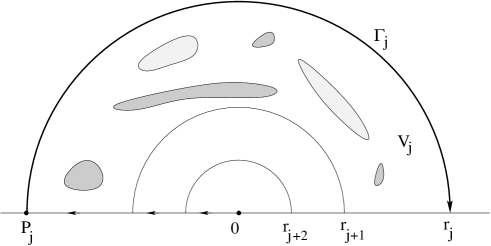
Figure 2: In dimension $d\geq 3$, if $\mu(V_{j})$ is large, then we can increase the payoff (3.1) by simply removing all the mass contained in the spherical shell $V_{j}$. This idea is used in step 3 of the proof of Theorem 3.1. In dimension $d=2$, if $\mu(V_{j})$ is large, to increase the payoff (3.1) we replace the measure $\mu_{j}=\chi_{V_{j}}\cdot\mu$ with a new measure $\tilde{\mu}_{j}$ uniformly distributed over the half circumference $\Gamma_{j}$. Notice that $\tilde{\mu}_{j}$ can be irrigated by moving the water particles from the origin to $P_{j}$, and then along $\Gamma_{j}\,$.

Theorem 3.2

If $d=2$ and $\alpha$ satisfies (3.30), then the unconstrained optimization problem (3.1) admits an optimal solution $\mu$, with bounded support and bounded total mass.

Indeed, repeating the steps 1 - 2 in the proof of the Theorem 3.1, we obtain a maximizing sequence $(\mu_{k})_{k\geq 1}$ of positive measures with uniformly bounded support. Moreover, the irrigation costs ${\cal I}^{\alpha}(\mu_{k})$ remain uniformly bounded.

In order to achieve a uniform bound on the total mass $\mu_{k}({\mathbb{R}}^{d})$, an auxiliary result is needed.

Lemma 3.3

Let $\alpha$ satisfy (3.30) and let $\kappa_{1}>0$ be given. Then there exists an integer $j^{*}$ and an exponent $\varepsilon>0$ such that the following holds. Given any bounded measure $\mu$ with ${\cal I}^{\alpha}(\mu)\leq\kappa_{1}$, there exists a second measure $\tilde{\mu}$ satisfying (3.28) and such that, setting $r_{j}\doteq 2^{-j}$,

$$\tilde{\mu}\Big{(}\bigl{\{}x\in{\mathbb{R}}^{2}\,;~{}~{}r_{j+1}<|x|\leq r_{j}\bigr{\}}\Big{)}~{}\leq~{}2^{-\varepsilon j}\qquad\qquad\hbox{for all}~{}j\geq j^{*}.$$ (3.31)

Proof. 1. If (3.30) holds, we can find $0<\varepsilon<\beta<1$ such that

$$\alpha\beta+1~{}>~{}\varepsilon+{1\over\alpha}\,.$$ (3.32)

Let $\mu_{j}$ be the restriction of the measure $\mu$ to the spherical shell $V_{j}$ defined at (3.22). Moreover, let $\tilde{\mu}_{j}$ be the positive measure with total mass

$$\tilde{\mu}_{j}({\mathbb{R}}^{d})~{}=~{}\pi r_{j}^{\,\beta},$$

uniformly distributed on the half circumference

$$\Gamma_{j}~{}\doteq~{}\{x=(x_{1},x_{2})\in{\mathbb{R}}^{2}\,;~{}~{}|x|=r_{j}\,,~{}x_{2}>0\}.$$

As shown in Fig. 2, there is a simple irrigation plan $\chi$ for $\tilde{\mu}_{j}$. Namely, we can first move all water particles on a straight line from the origin to the point $P_{j}=(-r_{j},0)$, then from $P_{j}$ to all points along the half circumference $\Gamma_{j}$. The total cost of this irrigation plan satisfies

$$\begin{array}[]{rl}{\cal E}^{\alpha}(\chi)&\leq~{}[\hbox{total mass}]^{\alpha}\times[\hbox{maximum length traveled}]\\[8.53581pt] &\leq~{}(\pi r_{j}^{\beta})^{\alpha}\cdot(\pi+1)r_{j}.\end{array}$$ (3.33)

Therefore, the minimum irrigation cost for $\tilde{\mu}_{j}$ satisfies

$${\cal I}^{\alpha}(\tilde{\mu}_{j})\leq~{}2\pi^{\alpha+1}\,r_{j}^{\alpha\beta+1}.$$ (3.34)

On the other hand, assuming $\mu(V_{j})\geq r_{j}^{\,\varepsilon}$, by (3.25) we have

$${\cal I}^{\alpha}(\mu)-{\cal I}^{\alpha}(\mu-\mu_{j})~{}\geq~{}{\kappa_{3}\over 4}r_{j}^{\varepsilon+{1\over\alpha}}.$$ (3.35)

By (3.32), for all $r_{j}$ small enough it follows

$$\Big{[}{\cal I}^{\alpha}(\mu)-{\cal I}^{\alpha}(\mu-\mu_{j})\Big{]}-{\cal I}^{\alpha}(\tilde{\mu}_{j})~{}\geq~{}{\kappa_{3}\over 8}r_{j}^{\varepsilon+{1\over\alpha}}.$$ (3.36)

Figure 3: Let $\tilde{\mu}_{j}$ be the measure supported on the half circumference $\Gamma_{j}$, with constant density $r_{j}^{\beta-1}$ w.r.t. 1-dimensional measure. Then, for any unit vector ${\bf n}$, the projected measure $\pi_{\bf n}\tilde{\mu}_{j}$ has density $\geq~{}r_{j}^{\beta-1}$ on $[a_{j},b_{j}]=\pi_{\bf n}(\Gamma_{j})$.

2. Next, we estimate how the sunlight functional changes if we replace $\mu_{j}$ by $\tilde{\mu}_{j}$. We claim that

$$\begin{array}[]{l}{\cal S}^{\eta}(\mu)-S^{\eta}(\mu-\mu_{j}+\tilde{\mu}_{j})\\[8.53581pt] \qquad\leq~{}[\hbox{total amount of light hitting $V_{j}$}]-[\hbox{light captured by $\tilde{\mu}_{j}$}]\\[8.53581pt] \qquad\leq~{}\|\eta\|_{{\bf L}^{1}}\cdot\exp\bigl{(}-r_{j}^{\beta-1}\bigr{)}.\end{array}$$ (3.37)

Indeed, consider any unit vector ${\bf n}\in S^{1}$. As shown in Fig. 3, let $[a_{j},b_{j}]=\pi_{\bf n}(\Gamma_{j})$ be the perpendicular projection of $\Gamma_{j}$ on the orthogonal subspace $E^{\perp}_{\bf n}$. By construction, the projected measure $\pi_{\bf n}\tilde{\mu}_{j}$ is absolutely continuous w.r.t. 1-dimensional Lebesgue measure on $E^{\perp}_{\bf n}$. Its density $\Phi_{j}^{\bf n}$ satisfies

$$\left\{\begin{array}[]{rll}\Phi_{j}^{\bf n}(y)&\geq~{}r_{j}^{\beta-1}&\hbox{if}~{}~{}y\in[a_{j},b_{j}],\\[5.69054pt] \Phi_{j}^{\bf n}(y)&=~{}0&\hbox{if}~{}~{}y\notin[a_{j},b_{j}].\end{array}\right.$$

For $j\geq 1$ we thus have

$$\begin{array}[]{l}[\hbox{total amount of light hitting $V_{j}$ in the direction ${\bf n}$}]\\[8.53581pt] \qquad\qquad-[\hbox{light parallel to ${\bf n}$ captured by $\tilde{\mu}_{j}$}]\\[8.53581pt] \displaystyle\qquad\leq~{}(b_{j}-a_{j})-\int_{a_{j}}^{b_{j}}\Big{(}1-e^{-\Phi_{j}^{\bf n}(y)}\Big{)}\,dy\\[8.53581pt] \displaystyle\qquad\leq~{}\int_{a_{j}}^{b_{j}}\exp\bigl{(}-r_{j}^{\beta-1}\bigr{)}\,dy~{}\leq~{}\exp\bigl{(}-r_{j}^{\beta-1}\bigr{)},\end{array}$$ (3.38)

because $b_{j}-a_{j}\leq 1$. 3. We now observe that, since $\beta<1$, when $j\geq j^{*}$ is sufficiently large the right hand side of (3.38) is smaller than the right hand side of (3.36). By possibly choosing a larger $j^{*}$, we can also assume that

$$\pi r_{j}^{\beta}~{}<~{}r_{j}^{\varepsilon}\qquad\hbox{for all}~{}j\geq j^{*}.$$ (3.39)

Defining the set of indices

$$J~{}\doteq~{}\bigl{\{}j\geq j^{*}\,;~{}~{}\mu(V_{j})~{}>~{}r_{j}^{\varepsilon}\bigr{\}},$$

we claim that the modified measure

$$\tilde{\mu}~{}\doteq~{}\mu+\sum_{j\in J}(\tilde{\mu}_{j}-\mu_{j}).$$ (3.40)

satisfies all conclusions of the lemma. Indeed, from (3.36) and (3.37)-(3.38) it follows that $\tilde{\mu}$ achieves a better payoff than $\mu$, i.e. (3.28) holds. In addition, the bounds (3.31) on the total mass follow from (3.39). MM     

We observe that (3.31) implies an a priori bound on the total mass $\tilde{\mu}\Big{(}\bigl{\{}x\in{\mathbb{R}}^{2}\,;~{}~{}|x|\leq r_{j^{*}}\bigr{\}}\Big{)}$. On the other hand, a bound on $\tilde{\mu}\Big{(}\bigl{\{}x\in{\mathbb{R}}^{2}\,;~{}~{}|x|\geq r_{j^{*}}\bigr{\}}\Big{)}$ is already provided by (3.12).

Thanks to the above lemma, the proof of Theorem 3.2 is now straightforward. Indeed, by Lemma 3.3 we can replace each $\mu_{k}$ by a new measure $\tilde{\mu}_{k}$ we can one can construct a maximizing sequence of measures with uniformly bounded support and uniformly bounded total mass. Taking a weak limit, the existence of an optimal solution can thus be proved using the upper semicontinuity of ${\cal S}^{\eta}$ and the lower semicontinuity of ${\cal I}^{\alpha}$, as in [8].

4 Optimal root configurations, without size constraint

In this section we study the optimal shape of tree roots.

• Optimization Problem for Roots.

  $$\hbox{maximize:}~{}~{}{\cal H}(u,\mu)-c{\cal I}^{\alpha}(\mu),$$ (4.1)

  subject to

  $$\left\{\begin{array}[]{rl}\Delta u+f(u)-u\mu&=~{}0,\qquad\qquad x\,\in\,{\mathbb{R}}^{d}_{-}\,\doteq\,\bigl{\{}(x_{1},\ldots,x_{d})\,;~{}~{}x_{d}<0\bigr{\}},\\[8.53581pt] u_{x_{d}}&=~{}0,\qquad\qquad x_{d}\,=\,0.\end{array}\right.$$ (4.2)

  Here $\mu$ is a positive measure concentrated on the set

  $$\Omega_{0}~{}\doteq~{}\bigl{\{}(x_{1},\ldots,x_{d})\not=(0,\ldots,0)\,;~{}~{}x_{d}\leq 0\bigr{\}},$$ (4.3)

  without any constraint on its total mass.

We recall that

$${\cal H}(u,\mu)~{}=~{}\int_{\{x_{d}\,\leq\,0\}}u\,d\mu~{}=~{}\int_{{\mathbb{R}}^{d}_{-}}f(u)\,dx$$ (4.4)

is the harvest functional introduced at (2.14), while ${\cal I}^{\alpha}(\mu)$ is the minimum irrigation cost defined at (2.21).

As in Section 2, we assume that the function $f$ satisfies all conditions in (2.15). In order to construct an optimal solution, we consider a maximizing sequence $(u_{k},\mu_{k})_{k\geq 1}$. By suitably adapting the arguments used in the previous section, we will prove a priori bounds on the total irrigation costs ${\cal I}^{\alpha}(\mu_{k})$ and on the total harvesting payoffs ${\cal H}(u_{k},\mu_{k})$. Our first lemma shows that the total harvest achieved by a measure supported on a closed ball $\overline{B}_{\rho}$, centered at the origin with a large radius $\rho$, grows at most like $\rho^{d}$.

Lemma 4.1

Let $f$ satisfy the assumptions (A1). Then there exists a constant $C_{f}$ such that the following holds. For any $\rho\geq 1$, if $\mu$ is a positive measure supported inside the closed ball $\overline{B}_{\rho}$, then for any solution $u$ of (4.2) one has

$${\cal H}(u,\mu)~{}\leq~{}C_{f}\,\rho^{d}.$$ (4.5)

Proof. 1. As shown in Fig. 4, right, let $\psi=\psi(r)$ be the solution to the ODE

$$\psi^{\prime\prime}(r)+f(\psi(r))~{}=~{}0,\qquad\qquad r>0,$$ (4.6)

$$\psi(0)~{}=~{}0,\qquad\qquad\lim_{r\to+\infty}\psi(r)~{}=~{}M.$$ (4.7)

We claim that $\psi$ is a monotonically increasing function such that

$$\psi(r)~{}\to~{}M\qquad\hbox{as}\qquad r\to+\infty,$$

with an exponential rate of convergence.

Indeed, let $F(s)=\int_{0}^{s}f(\xi)\,d\xi$. Then, for any solution of (4.6), the energy

$$E(r)~{}\doteq~{}{\bigl{(}\psi^{\prime}(r)\bigr{)}^{2}\over 2}+F\bigl{(}\psi(r)\bigr{)}$$ (4.8)

is constant. The second limit in (4.7) implies that $E=F(M)$. We thus obtain the ODE

$$\psi^{\prime}(r)~{}=~{}\sqrt{2F(M)-2F(\psi(r))}.$$ (4.9)

Since $f(M)=0$ and $f^{\prime}(M)<0$, for $\psi\in[0,M]$ one has

$$F(M)-F(\psi)~{}\geq~{}\gamma\,(M-\psi)^{2},$$ (4.10)

for some constant $\gamma>0$ depending only on $f$ itself. Therefore,

$$\psi^{\prime}(r)~{}>~{}\sqrt{2\gamma}(M-\psi)$$

We thus conclude that the solution $\psi$ of (4.6)-(4.7) satisfies

$$\psi(r)~{}\geq~{}M(1-e^{-\sqrt{2\gamma}\,r}).$$ (4.11)

Therefore

$$f(\psi(r))~{}\leq~{}f^{{}^{\prime}}(M)(\psi(r)-M)~{}\leq~{}C_{1}e^{-\sqrt{2\gamma}\,r}\,,\qquad C_{1}~{}\doteq~{}-f^{{}^{\prime}}(M)M>0\,.$$ (4.12)

2. Let $u$ be a solution to (2.8)-(2.9), where the measure $\mu$ is supported on the ball $\overline{B}_{\rho}$. We claim that $u\geq v$, where $v$ is the radially symmetric function defined by

$$v(x)~{}=~{}\left\{\begin{array}[]{cl}\psi(|x|-\rho)&\hbox{if}~{}~{}|x|\geq\rho,\\[8.53581pt] 0&\hbox{if}~{}~{}|x|<\rho.\end{array}\right.$$ (4.13)

Indeed, for $|x|>\rho$, by (4.13) and (4.6) one has

$$\begin{array}[]{ll}\Delta v(x)+f(v)&\displaystyle=~{}\psi^{\prime\prime}(|x|-\rho)+\frac{d-1}{|x|}\psi^{\prime}(|x|-\rho)+f\bigl{(}\psi(|x|-\rho)\bigr{)}\\[8.53581pt] &\displaystyle=~{}\frac{d-1}{|x|}\psi^{\prime}(|x|-\rho)~{}\geq~{}0,\end{array}$$ (4.14)

showing that $v$ is a lower solution on the region where $|x|>\rho$. Hence $u(x)\geq v(x)$ for all $x\in{\mathbb{R}}^{d}$. 3. Since $u\geq v$, an upper bound on the total harvest is now provided by:

$${\cal H}(u,\mu)~{}=~{}\int_{\Omega}f(u(x))\,dx~{}\leq~{}{\omega_{d-1}\over 2}\,\int_{0}^{+\infty}r^{d-1}\widehat{f}(\psi(r-\rho))\,dr,$$ (4.15)

where (see Fig. 4, left)

$$\widehat{f}(s)~{}=~{}\max\bigl{\{}f(\xi)\,;~{}~{}\xi\in[s,M]\bigr{\}}~{}=~{}\left\{\begin{array}[]{cl}f(s)&\hbox{if}~{}~{}s\geq u_{max}\,,\\[5.69054pt] K&\hbox{if}~{}~{}s\leq u_{max}\,.\end{array}\right.$$ (4.16)

Here $u_{max}\in\,]0,M[\,$ is the unique point at which the function $f$ attains its maximum. 4. By the previous steps, the solution $\psi$ of (4.6)-(4.7) is a monotonically increasing function converging to $M$ as $s\to+\infty$. We can thus find a radius $r^{*}>1$ large enough so that

$$\psi(r)~{}\geq~{}u_{max}\qquad\qquad\hbox{for all}~{}r\geq r^{*}.$$ (4.17)

Indeed, one can choose

$$r^{*}~{}\doteq~{}-\frac{\ln(1-\frac{u_{max}}{M})}{\sqrt{2\gamma}}\,.$$ (4.18)

Using (4.16),(4.12) and performing the variable change $r=\rho+s$, one finds

$$\begin{array}[]{rl}\displaystyle\int_{0}^{\infty}r^{d-1}\widehat{f}(\psi(r-\rho))dr&\displaystyle=~{}\int_{0}^{\rho+r^{*}}r^{d-1}f(u_{max})\,dr+\int_{\rho+r^{*}}^{+\infty}r^{d-1}f(\psi(r-\rho))\,dr\\[11.38109pt] &\displaystyle\leq~{}\frac{K}{d}(\rho+r^{*})^{d}+\int_{\rho+r^{*}}^{+\infty}r^{d-1}C\,e^{-\sqrt{2\gamma}(r-\rho)}\,dr\\[11.38109pt] &\displaystyle\leq~{}\frac{K}{d}(\rho+r^{*})^{d}+\rho^{d-1}\int_{r^{*}}^{+\infty}(1+s)^{d-1}C\,e^{-\sqrt{2\gamma}\,s}\,ds\\[11.38109pt] &\leq~{}C_{1}\rho^{d}+C_{2}\rho^{d-1}.\end{array}$$ (4.19)

Combining (4.19) with (4.15) one obtains the desired inequality (4.5). MM     

The next lemma provides an estimate on the total harvest achieved by a measure supported in a small ball $\overline{B}_{\rho}$, as $\rho\to 0$.

Lemma 4.2

Let $f$ satisfy (A1). Then there exists a positive continuous function $\eta$, with $\lim_{s\to 0+}\eta(s)=0$, such that the following holds. Let $(u,\mu)$ be any solution of (4.2). If $\mu$ is supported on the closed ball $\overline{B}_{\rho}$, then the total harvest satisfies

$${\cal H}(u,\mu)~{}\leq~{}\eta(\rho).$$ (4.20)

Proof. 1. Let $U=U(r)$ be a solution to

$$U^{\prime\prime}(r)+{d-1\over r}U^{\prime}(r)+f(U)~{}=~{}0,\qquad\qquad\rho<r<+\infty,$$ (4.21)

$$U(\rho)~{}=~{}0,\qquad\qquad\lim_{r\to+\infty}U(r)~{}=~{}M.$$ (4.22)

A lower bound on $U$ will be achieved by constructing a suitable subsolution.

Observing that $f(U)\geq 0$ and $U^{\prime}>0$, such a subsolution can be obtained by patching together a solution to

$$U^{\prime\prime}(r)+{d-1\over r}U^{\prime}(r)~{}=~{}0,\qquad\qquad\rho<r<r^{*},$$ (4.23)

with a solution of

$$U^{\prime\prime}(r)+f(U)~{}=~{}0,\qquad\qquad r^{*}<r<+\infty.$$ (4.24)

As in the proof of the previous lemma, let $\psi$ be the solution to (4.6) and (4.7). In addition, a solution of (4.23) with boundary condition

$$U(\rho)~{}=~{}0$$ (4.25)

is found in the form

$$U(r)~{}=~{}\left\{\begin{array}[]{cl}\kappa\,(\ln r-\ln\rho)&\hbox{if}~{}~{}d=2,\\[8.53581pt] \kappa(\rho^{\,2-d}-r^{2-d})&\hbox{if}~{}~{}d\geq 3.\end{array}\right.$$ (4.26)

By linearity, here $\kappa$ can be any constant.

 

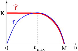
Figure 4: Left: a function $f$ satisfying the assumptions (2.15) and the corresponding function $\widehat{f}$ in (4.16). Right: a subsolution obtained by patching together the functions $U_{\varepsilon}$ and $\psi$.

2. To patch together the two solutions $U$ and $\psi$, we proceed as follows. Recalling (4.16), for any $\varepsilon>0$, choose $R_{\varepsilon}$ large enough so that

$$R_{\varepsilon}\,\bigl{(}\psi(R_{\varepsilon})-M\bigr{)}~{}<~{}\varepsilon,\qquad\qquad\int_{R_{\varepsilon}}^{+\infty}\widehat{f}(\psi(s))\,ds~{}\leq~{}\varepsilon.$$ (4.27)

This is certainly possible because $f(M)=0$ and $\psi(s)\to M$ exponentially fast as $s\to+\infty$. Next, we claim that there exists $r_{\varepsilon}>0$ small enough and $\kappa_{\varepsilon}>0$ so that the function

$$U_{\varepsilon}(r)~{}\doteq~{}\left\{\begin{array}[]{cl}\kappa_{\varepsilon}\,(\ln r-\ln r_{\varepsilon})&\hbox{if}~{}~{}d=2,\\[8.53581pt] \kappa_{\varepsilon}(r_{\varepsilon}^{\,2-d}-r^{2-d})&\hbox{if}~{}~{}d\geq 3,\end{array}\right.$$ (4.28)

satisfies (see Fig. 4, right)

$$U_{\varepsilon}(R_{\varepsilon})~{}=~{}\psi(R_{\varepsilon}),\qquad\qquad U^{\prime}_{\varepsilon}(R_{\varepsilon})~{}\leq~{}\psi^{\prime}(R_{\varepsilon}),$$ (4.29)

$$Kr_{\varepsilon}+\int_{r_{\varepsilon}}^{R_{\varepsilon}}\widehat{f}(U_{\varepsilon}(s))\,ds~{}<~{}\varepsilon.$$ (4.30)

Here $K$ is the maximum value of $f$, as in (2.15).

To prove our claim, having fixed $R_{\varepsilon}$, for any $\rho>0$ we determine $\kappa_{\varepsilon}$ so that the function

$$U_{\rho}(r)~{}\doteq~{}\left\{\begin{array}[]{cl}\kappa_{\varepsilon}\,(\ln r-\ln\rho)&\hbox{if}~{}~{}d=2,\\[8.53581pt] \kappa_{\varepsilon}(\rho^{\,2-d}-r^{2-d})&\hbox{if}~{}~{}d\geq 3,\end{array}\right.$$ (4.31)

satisfies $U_{\rho}(R_{\varepsilon})=\psi(R_{\varepsilon})$. As $\rho\to 0$, one now has

$$\lim_{\rho\to 0}U^{\prime}_{\rho}(R_{\varepsilon})~{}=~{}0,\qquad\qquad\lim_{\rho\to 0}U_{\rho}(r)~{}=~{}\psi(R_{\varepsilon})\qquad\hbox{for any}~{}0<r\leq R_{\varepsilon}.$$ (4.32)

This is proved by a direct computation. When $d=2$ we have

$$\kappa_{\varepsilon}~{}=~{}{\psi(R_{\varepsilon})\over\ln R_{\varepsilon}-\ln\rho}\,,\qquad\quad U_{\rho}(r)~{}=~{}\psi(R_{\varepsilon})\,{\ln r-\ln\rho\over\ln R_{\varepsilon}-\ln\rho}\,,$$

$$U^{\prime}_{\rho}(r)~{}=~{}{1\over r}\,{\psi(R_{\varepsilon})\over\ln R_{\varepsilon}-\ln\rho}\,.$$

Hence the limits in (4.32) hold. On the other hand, when $d\geq 3$ we have

$$\kappa_{\varepsilon}~{}=~{}{\psi(R_{\varepsilon})\over R_{\varepsilon}^{2-d}-\rho^{2-d}}\,,\qquad\quad U_{\rho}(r)~{}=~{}\psi(R_{\varepsilon})\,{\rho^{2-d}-r^{2-d}\over\rho^{2-d}-R_{\varepsilon}^{2-d}}\,,$$

$$U^{\prime}_{\rho}(r)~{}=~{}{\psi(R_{\varepsilon})}{(d-2)r^{1-d}\over\rho^{2-d}-R_{\varepsilon}^{2-d}}\,,$$

and the limits in (4.32) again hold. Having determined $R_{\varepsilon}$ according to (4.27), if we now choose $r_{\varepsilon}=\rho>0$ small enough, by the first limit in (4.32) it follows $U_{\varepsilon}^{\prime}(R_{\varepsilon})<\psi^{\prime}(R_{\varepsilon})$.

Moreover, thanks to the second limit in (4.32) and the first inequality in (4.27), by choosing $r_{\varepsilon}>0$ small enough we also achieve

$$Kr_{\varepsilon}+\int_{r_{\varepsilon}}^{R_{\varepsilon}}\widehat{f}(U_{\varepsilon}(s))\,ds~{}<~{}\varepsilon+R_{\varepsilon}f(\psi(R_{\varepsilon}))~{}\leq~{}\varepsilon+R_{\varepsilon}\,L_{f}(\psi(R_{\varepsilon})-M)~{}\leq~{}(L_{f}+1)\varepsilon\,,$$

where $L_{f}$ denotes the Lipschitz constant of $f$. Since $\varepsilon>0$ was arbitrary, our claim is proved. 3. Let $u$ be a solution to (4.2), where the measure $\mu$ is supported on the closed ball $\overline{B}_{\rho}$. By a comparison argument, we conclude that $u\geq v$, where $v$ is the function defined by

$$v(x)~{}=~{}\left\{\begin{array}[]{cl}0&\hbox{if}~{}~{}|x|\leq r_{\varepsilon}\,,\\[8.53581pt] U_{\varepsilon}(r)&\hbox{if}~{}~{}r_{\varepsilon}<|x|<R_{\varepsilon}\,,\\[8.53581pt] \psi(r)&\hbox{if}~{}~{}R_{\varepsilon}\leq|x|\,.\end{array}\right.$$

By (4.27)-(4.30), an upper bound on the total harvest is now provided by

$$\begin{array}[]{rl}{\cal H}(u,\mu)&\displaystyle=~{}\int_{{\mathbb{R}}^{d}_{-}}f(u(x))\,dx~{}\leq~{}{\omega_{d-1}\over 2}\,\int_{0}^{+\infty}r^{d-1}\widehat{f}(v(r))\,dr\\[11.38109pt] &\displaystyle=~{}{\omega_{d-1}\over 2}\left(\int_{0}^{r_{\varepsilon}}\widehat{f}(0)\,dr+\int_{r_{\varepsilon}}^{R_{\varepsilon}}U_{\varepsilon}(r)\,dr+\int_{R_{\varepsilon}}^{+\infty}\psi(r)\,dr\right)~{}\leq~{}\omega_{d-1}\,\varepsilon\,.\end{array}$$

Since $\varepsilon>0$ was arbitrary, this achieves the proof. MM     

Corollary 4.3

In the same setting as Lemma 4.2, let $\mu$ be a positive measure on ${\mathbb{R}}^{d}$ and let $(u,\mu)$ be a solution to (4.2). Then, for every $\rho>0$, one has

$$\int_{|x|\leq\rho}u\,d\mu~{}\leq~{}\eta(\rho),$$ (4.33)

where $\eta$ is the function in (4.20).

Proof. Call $\mu^{\rho}\doteq\chi_{\{|x|\leq\rho\}}\cdot\mu$ the restriction of the measure $\mu$ to the closed ball of radius $\rho$. Let $u^{\rho}\geq u$ be a corresponding solution of (4.2). Using Lemma 4.2 we now obtain

$$\int_{|x|\leq\rho}u\,d\mu~{}=~{}\int u\,d\mu^{\rho}~{}\leq~{}\int u^{\rho}\,d\mu^{\rho}~{}\leq~{}\eta(\rho).$$

MM     

Using Lemma 4.1, we now prove that an analogue of (3.9) holds also for the harvesting problem.

Lemma 4.4

Let $\alpha>1-{1\over d}$. Under the assumptions (A1), there exists a constant $\kappa_{1}$ such that, for any positive bounded measure $\mu$ on $\overline{\Omega}\doteq\{x=(x_{1},\ldots,x_{d})\in{\mathbb{R}}^{d}\,;~{}~{}x_{d}\leq 0\}$,

$${\cal I}^{\alpha}(\mu)~{}\geq~{}\kappa_{1}\qquad\Longrightarrow\qquad{\cal H}(u,\mu)-c{\cal I}^{\alpha}(\mu)~{}\leq~{}0.$$ (4.34)

Proof. Given any radius $r\geq 1$, we can decompose the measure $\mu$ as

$$\mu~{}=~{}\mu_{r}^{-}+\mu_{r}^{+}~{}\doteq~{}\chi_{\{x\leq r\}}\cdot\mu+\chi_{\{x>r\}}\cdot\mu\,$$ (4.35)

Let $u$ be a corresponding solution of (4.2). $0\leq u(x)\leq M$. Then there exists a solution $u^{-}$ to the same elliptic problem with $\mu$ replaced by $\mu_{r}^{-}$, such that

$$0~{}\leq~{}u(x)~{}\leq~{}u^{-}(x)\qquad\qquad\hbox{for all}~{}x\in{\mathbb{R}}^{d}_{-}\,.$$ (4.36)

Using (4.36), and recalling that $\mu$ is concentrated on the domain $\Omega_{0}$ at (4.3), the harvest functional can be estimated by

$$\begin{array}[]{rl}{\cal H}(u,\mu){}&\displaystyle\doteq~{}\int_{\Omega_{0}}u\,d\mu~{}=~{}\int_{\Omega_{0}}u\,d\mu_{r}^{-}+\int_{\Omega_{0}}u\,d\mu_{r}^{+}\\[11.38109pt] &\displaystyle\leq~{}\int_{\Omega_{0}}u^{-}\,d\mu_{r}^{-}~{}+~{}M\mu_{r}^{+}(\Omega_{0})\\[11.38109pt] &\displaystyle\leq~{}C_{f}\,r^{d}~{}+~{}M\Big{(}\frac{{\cal I}^{\alpha}(\mu)}{r}\Big{)}^{\frac{1}{\alpha}}.\end{array}$$ (4.37)

Here the last inequality was obtained by applying (4.5) to the measure $\mu_{r}^{-}$ and (2.24) to the measure $\mu^{+}_{r}$.

Next, assuming ${\cal I}^{\alpha}(\mu)$ sufficiently large, we can find a radius $\rho\geq 1$ such that

$$C_{f}\,\rho^{d}~{}=~{}M\Big{(}\frac{{\cal I}^{\alpha}(\mu)}{\rho}\Big{)}^{\frac{1}{\alpha}}.$$ (4.38)

Choosing $r=\rho$ in (4.37), we obtain

$${\cal H}(u,\mu)~{}\leq~{}C_{0}\Big{(}{\cal I}^{\alpha}(\mu)\Big{)}^{\frac{d}{1+\alpha d}}.$$ (4.39)

for some constant $C_{0}$ depending only on $\alpha,d,$ and $f$.

In connection with the original problem (4.1), this implies

$${\cal H}(u,\mu)-c{\cal I}^{\alpha}(\mu)~{}\leq~{}C_{0}\Big{(}{\cal I}^{\alpha}(\mu)\Big{)}^{\frac{d}{1+\alpha d}}-c{\cal I}^{\alpha}(\mu).$$ (4.40)

Assuming that $\alpha>1-\frac{1}{d}$, it follows that $\frac{d}{1+\alpha d}<1$. Hence by (4.40) there exists a constant $\kappa_{1}$ large enough so that (4.34) holds. MM     

Lemma 4.5

Let $\alpha>1-{1\over d}$ and let the assumptions (A1) hold. Consider a maximizing sequence $(u_{k},\mu_{k})_{k\geq 1}$ for the functional in (4.1). Then there exists another maximizing sequence $(\tilde{u}_{k},\tilde{\mu}_{k})_{k\geq 1}$ such that

$${\cal I}^{\alpha}(\tilde{\mu}_{k})~{}\leq~{}\kappa_{1}\,,\qquad\qquad{\cal H}(\tilde{u}_{k},\tilde{\mu}_{k})~{}\leq~{}\kappa_{2}\,,$$ (4.41)

for some constants $\kappa_{1},\kappa_{2}$ and all $k\geq 1$. Moreover, all measures $\tilde{\mu}_{k}$ are supported in a common ball $\overline{B}_{\rho}$.

Proof. 1. By (4.34), any maximizing sequence must satisfy the first inequality in (4.41). The second inequality then follows from (4.39). 2. It remains to prove the existence of a maximizing sequence with uniformly bounded support. Toward this goal, let $\chi$ be an optimal irrigation plan for a measure $\mu$. By (2.24) and (3.10), for any radius $r>0$ one has

$$\mu\Big{(}\{x\in{\mathbb{R}}^{d};~{}|x|\geq r\}\Big{)}~{}\leq~{}\Big{(}\frac{{\cal I}^{\alpha}(\mu)}{r}\Big{)}^{1/\alpha}~{}\leq~{}\Big{(}\frac{\kappa_{1}}{r}\Big{)}^{1/\alpha}.$$ (4.42)

Consider two radii $0<r_{1}<r_{2}$, where $r_{1}$ large enough such that (3.16) holds. As in (4.43), we can decompose the measure $\mu$ as a sum:

$$\mu~{}=~{}\mu^{-}+\mu^{+}~{}\doteq~{}\chi_{\{x\leq r_{2}\}}\cdot\mu+\chi_{\{x>r_{2}\}}\cdot\mu\,.$$ (4.43)

By the same argument used in (3.18), for $0<\alpha\leq 1$, one has

$${\cal I}^{\alpha}(\mu^{-}+\mu^{+})~{}-~{}{\cal I}^{\alpha}(\mu^{-})~{}\geq~{}(r_{2}-r_{1})\mu^{+}(\Omega_{0})\,,$$ (4.44)

where $\Omega_{0}$ is the domain in (4.3). 3. We now estimate the decrease in the harvest functional, when $\mu$ is replaced by $\mu^{-}$. Let $u$ be a solution of (4.2), corresponding to the measure $\mu$. Then there exists a solution $u^{-}$ to the same problem, with $\mu$ replaced by $\mu^{-}$, such that

$$0~{}\leq~{}u(x)~{}\leq~{}u^{-}(x)\qquad\quad\hbox{\hbox{for all}~{}}x\in{\mathbb{R}}^{d}_{-}\,.$$ (4.45)

Using (4.45), the harvest functional can be estimated by

$$\begin{array}[]{rl}{\cal H}(u,\mu){}&\displaystyle\doteq~{}\int_{\Omega_{0}}u\,d\mu~{}=~{}\int_{\Omega_{0}}u\,d\mu^{-}+\int_{\Omega_{0}}u\,d\mu^{+}\\[11.38109pt] &\displaystyle\leq~{}\int_{\Omega_{0}}u^{-}\,d\mu^{-}+\int_{\Omega_{0}}M\,d\mu^{+}\\[11.38109pt] &\displaystyle=~{}{\cal H}(u^{-},\mu^{-})~{}+~{}M\mu^{+}(\Omega_{0}).\end{array}$$ (4.46)

Taking $r_{2}$ large enough so that $c(r_{2}-r_{1})\geq M$, by (4.44) and (4.46) it follows

$${\cal H}(u,\mu)-{\cal H}(u^{-},\mu^{-})~{}\leq~{}c\Big{(}{\cal I}^{\alpha}(\mu)-{\cal I}^{\alpha}(\mu^{-})\Big{)}.$$ (4.47)

4. Let now $(u_{k},\mu_{k})_{k\geq 1}$ be a maximizing sequence. We decompose each measure as

$$\mu_{k}~{}=~{}\mu_{k}^{-}+\mu_{k}^{+}~{}\doteq~{}\chi_{\{x\leq r_{2}\}}\cdot\mu_{k}+\chi_{\{x>r_{2}\}}\cdot\mu_{k}\,.$$ (4.48)

Choose $u^{-}_{k}$ the corresponding solution to the same elliptic problem with $\mu_{k}$ replaced by $\mu_{k}^{-}$, such that

$$0~{}\leq~{}u_{k}(x)~{}\leq~{}u_{k}^{-}(x)\qquad\quad\hbox{\hbox{for all}~{}}x\in{\mathbb{R}}^{d}_{-}\,.$$ (4.49)

By (4.47), $(u_{k}^{-},\mu^{-}_{k})_{k\geq 1}$ is still a maximizing sequence, where all measures are supported inside the closed ball $\overline{B}_{r_{2}}$. MM     

The next lemma yields a more detailed estimate on the support of the optimal measure.

Lemma 4.6

Suppose $(u_{k},\mu_{k})_{k\geq 1}$ is a maximizing sequence for the optimization problem (4.1), with irrigation costs ${\cal I}^{\alpha}(\mu_{k})\leq\kappa_{1}$ for all $k\geq 1$. Then there exists a second maximizing sequence $(\tilde{u}_{k},\tilde{\mu}_{k})_{k\geq 1}$ such that

$$\tilde{\mu}_{k}\Big{(}\bigl{\{}x\in{\mathbb{R}}^{d}\,;\quad\tilde{u}_{k}(x)~{}<~{}C_{0}|x|^{1/\alpha}\,\bigr{\}}\Big{)}~{}=~{}0$$ (4.50)

for all $k\geq 1$. Here $C_{0}\doteq c\,2^{-\frac{1}{\alpha}}\,\kappa_{1}^{1-\frac{1}{\alpha}}$.

Proof. 1. Given a positive measure $\mu$ and a corresponding solution $u$ of (4.2), consider the set

$$A~{}\doteq~{}\bigl{\{}x\in\Omega_{0}\,;\qquad u(x)~{}\geq~{}C_{0}|x|^{1/\alpha}\bigr{\}}.$$

Moreover, let

$$\tilde{\mu}~{}\doteq~{}\chi_{A}\cdot\mu$$ (4.51)

be the measure obtained from $\mu$ by removing all the mass that lies outside $A$.

By (3.25) it follows

$$c{\cal I}^{\alpha}(\mu)-c{\cal I}^{\alpha}(\tilde{\mu})~{}\geq~{}C_{0}\int_{\Omega_{0}\setminus A}|x|^{1/\alpha}\,d\mu,$$ (4.52)

2. To estimate the difference in the harvest functional, let $\tilde{u}$ be a solution to the same elliptic problem (4.2) with $\mu$ replaced by $\tilde{\mu}$, such that

$$u(x)~{}\leq~{}\tilde{u}(x)~{}\leq~{}M\,\qquad\hbox{for all}~{}x\in\overline{\Omega}\,.$$ (4.53)

We compute

$${\cal H}(u,\mu)-{\cal H}(\tilde{u},\tilde{\mu})~{}=~{}\int_{\Omega_{0}}u\,d\mu-\int_{\Omega_{0}}\tilde{u}\,d\tilde{\mu}~{}\leq~{}\int_{\Omega_{0}\setminus A}u\,d\mu~{}\leq~{}C_{0}\int_{\Omega_{0}\setminus A}|x|^{1/\alpha}\,d\mu\,.$$ (4.54)

Comparing (4.52) with (4.54) we thus obtain

$${\cal H}(u,\mu)-c{\cal I}^{\alpha}(\mu)~{}\leq~{}{\cal H}(\tilde{u},\tilde{\mu})-c{\cal I}^{\alpha}(\tilde{\mu}).$$ (4.55)

Recalling that $u\leq\tilde{u}$, by (4.51) it follows

$$\tilde{\mu}\Big{(}\bigl{\{}x\in\Omega_{0}\,;\quad\tilde{u}(x)~{}<~{}C_{0}|x|^{1/\alpha}\,\bigr{\}}\Big{)}~{}\leq~{}\tilde{\mu}\Big{(}\bigl{\{}x\in\Omega_{0}\,;\quad u(x)~{}<~{}C_{0}|x|^{1/\alpha}\,\bigr{\}}\Big{)}~{}=~{}0.$$

3. If now $(u_{k},\mu_{k})_{k\geq 1}$ is any maximizing sequence, for every $k\geq 1$ we define

$$A_{k}~{}\doteq~{}\bigl{\{}x\in\overline{\Omega}\,;\qquad u_{k}(x)~{}\geq~{}C_{0}|x|^{1/\alpha}\bigr{\}},\qquad\tilde{\mu}_{k}~{}\doteq~{}\chi_{A_{k}}\cdot\mu_{k}\,.$$

Moreover, we let $\tilde{u}_{k}\geq u_{k}$ be a solution to (4.2) corresponding to the measure $\tilde{\mu}_{k}$. By the previous analysis, $(\tilde{u}_{k},\tilde{\mu}_{k})_{k\geq 1}$ is another maximizing sequence, satisfying (4.50). MM     

When $f$ satisfies the assumptions (2.15), any solution $u$ of (2.8) will take values inside the interval $[0,M]$. By the previous arguments, it thus follows the existence of a maximizing sequence $(u_{k},\mu_{k})_{k\geq 1}$, where the measures $\mu_{k}$ satisfy

• Supp$(\mu_{k})\subset\overline{B}_{r_{0}}$, where $C_{0}r_{0}^{1/\alpha}=M$.

• ${\cal I}^{\alpha}(\mu_{k})\leq C$.

In particular, for every $r>0$ one has

$$\sup_{k\geq 1}~{}\mu_{k}\bigl{(}\{x\in{\mathbb{R}}^{d}\,;~{}|x|>r\}\bigr{)}~{}<~{}+\infty.$$ (4.56)

This does not necessarily imply that the total mass of the measures $\mu_{k}$ is uniformly bounded. Indeed, they may concentrate more and more mass close to the origin.

To achieve the existence of an optimal measure, we thus need to work in the wider class of positive measures $\mu$ on the domain $\Omega_{0}$ in (4.3), possibly with infinite total mass. As a preliminary, the definition of irrigation plan and irrigation cost must be extended to these more general measures.

If $\mu({\mathbb{R}}^{d})=+\infty$, an irrigation plan for $\mu$ is a map $\chi:{\mathbb{R}}_{+}\times{\mathbb{R}}_{+}\mapsto{\mathbb{R}}^{d}$ with the properties (i)–(iii) introduced in Section 1. For every $m\geq 1$, call $\chi_{m}:[0,m]\times{\mathbb{R}}_{+}\mapsto{\mathbb{R}}^{d}$ the restriction of $\chi$ to $[0,m]$. Then the cost of $\chi$ is defined as

$${\cal E}^{\alpha}(\chi)~{}\doteq~{}\lim_{m\to+\infty}{\cal E}^{\alpha}(\chi_{m})~{}=~{}\sup_{m\geq 1}\int_{0}^{m}\int_{0}^{\tau(\theta)}\bigl{|}\chi_{m}(\theta,t)\bigr{|}_{\chi_{m}}^{\alpha-1}\,dtd\theta.$$ (4.57)

On the other hand, the harvest functional is defined as

$${\cal H}(u,\mu)~{}\doteq~{}\sup_{\varepsilon\to 0+}~{}\int_{|x|>\varepsilon}u\,d\mu\,.$$ (4.58)

It is clear that the right hand sides in (4.57) and (4.58) are well defined, possibly taking the value $+\infty$.

We can now state our main result on the existence of an optimal measure.

Theorem 4.7

Let the function $f$ satisfy the assumptions (A1). Then the maximization problem for roots (OPR) has an optimal solution $(u,\mu)$, where $\mu$ is a positive measure on the domain $\Omega_{0}$ defined at (4.3). The optimal measure $\mu$ has bounded support, but possibly unbounded total mass.

Proof. 1. Let $(u_{k},\mu_{k})$ be a maximizing sequence. By the previous analysis we can assume that all measures $\mu_{k}$ are supported inside a fixed ball $\overline{B}_{\rho}$, and the quantities ${\cal I}^{\alpha}(\mu_{k})$, ${\cal H}(u_{k},\mu_{k})$ remain uniformly bounded.

By possibly selecting a subsequence, we can assume the existence of a positive measure $\mu$ such that the weak convergence $\mu_{k}\rightharpoonup\mu$ holds on ${\mathbb{R}}^{d}\setminus\{0\}$. In other words,

$$\int\varphi\,d\mu_{k}~{}\to~{}\int\varphi\,d\mu$$

for every continuous function $\varphi\in{\cal C}_{c}({\mathbb{R}}^{d}\setminus\{0\})$.

Let $\mu^{\varepsilon}$ be the restriction of $\mu$ to the subset $\{|x|>\varepsilon\}$. Then

$${\cal I}^{\alpha}(\mu)~{}=~{}\sup_{\varepsilon>0}~{}{\cal I}^{\alpha}(\mu^{\varepsilon}).$$ (4.59)

On the other hand, calling $\mu^{\varepsilon}_{k}$ the restriction of $\mu_{k}$ to the set $\{|x|\geq\varepsilon\}$, the lower semicontinuity of the irrigation cost for bounded measures implies

$${\cal I}^{\alpha}(\mu^{\varepsilon})~{}\leq~{}\liminf_{m\to\infty}~{}{\cal I}^{\alpha}(\mu^{\varepsilon}_{k})~{}\leq~{}\liminf_{m\to\infty}~{}{\cal I}^{\alpha}(\mu_{k}).$$ (4.60)

Combining (4.59) with (4.60) we obtain

$${\cal I}^{\alpha}(\mu)~{}\leq~{}\liminf_{m\to\infty}~{}{\cal I}^{\alpha}(\mu_{k}).$$ (4.61)

2. To complete the existence proof, we need to find a solution $u$ of (4.2) and show that

$${\cal H}(u,\mu)~{}\geq~{}\limsup_{k\to\infty}~{}{\cal H}(u_{k},\mu_{k}).$$ (4.62)

Toward this goal, choose radii $\rho_{n}\to 0$ such that

$$\mu\Big{(}\{x\in\Omega_{0}\,;~{}~{}|x|=\rho_{n}\}\Big{)}~{}=~{}0$$ (4.63)

for all $n\geq 1$. Let $\mu^{\rho_{n}}_{k},\mu^{\rho_{n}}$ be the restrictions of the measures $\mu_{k},\mu$ to the closed sets

$$V_{n}~{}\doteq~{}\{x\in\Omega_{0}\,;~{}~{}|x|\geq\rho_{n}\}.$$

Thanks to (4.63), for each $n\geq 1$ we have the weak convergence $\mu^{\rho_{n}}_{k}\rightharpoonup\mu^{\rho_{n}}$. Let $u^{\rho_{n}}_{k},u^{\rho_{n}}$ be the corresponding solutions of (4.2). By the analysis in [8], since all measures $\mu_{k}^{\rho_{n}}$ have uniformly bounded mass, for each $n\geq 1$ we have

$$\int u^{\rho_{n}}\,d\mu^{\rho_{n}}~{}\geq~{}\limsup_{k\to\infty}\int u^{\rho_{n}}_{k}\,d\mu^{\rho_{n}}_{k}\,.$$ (4.64)

By Corollary 4.3 it follows

$$\int u_{k}\,d\mu_{k}~{}\leq~{}\int u^{\rho_{n}}_{k}\,d\mu^{\rho_{n}}_{k}+\eta(\rho_{n}).$$ (4.65)

3. We now observe that, as $n\to\infty$, the sequence of measures $\mu^{\rho_{n}}$ is increasing while the sequence of solutions $u^{\rho_{n}}$ is decreasing. Setting

$$u(x)~{}\doteq~{}\inf_{n\geq 1}u^{\rho_{n}}(x),$$

one checks that $(u,\mu)$ is a solution to (4.2). Moreover, for any $\delta>0$ one has

$$\int_{|x|\geq\delta}u\,d\mu~{}=~{}\inf_{n\geq 1}\int_{|x|\geq\delta}u^{\rho_{n}}\,d\mu.$$ (4.66)

Given $\varepsilon>0$, we can find $\delta>0$ and then an integer $\widehat{n}$ large enough so that

$$\rho_{\widehat{n}}~{}\leq~{}\delta,\qquad\eta(\rho_{\widehat{n}})~{}\leq~{}\eta(\delta)~{}<~{}\varepsilon,\qquad\qquad\int_{|x|\geq\delta}u^{\rho_{\widehat{n}}}\,d\mu~{}<~{}\int_{|x|\geq\delta}u\,d\mu+\varepsilon\,.$$ (4.67)

Using (4.65), then (4.64), and finally (4.67), we conclude

$$\begin{array}[]{l}\displaystyle\limsup_{k\to\infty}\int u_{k}\,d\mu_{k}~{}\leq~{}\limsup_{k\to\infty}\int u_{k}^{\rho_{\widehat{n}}}\,d\mu_{k}^{\rho_{\widehat{n}}}+\eta(\rho_{\widehat{n}})~{}\leq~{}\int u^{\rho_{\widehat{n}}}\,d\mu^{\rho_{\widehat{n}}}+\eta(\rho_{\widehat{n}})\\[11.38109pt] \displaystyle\qquad<~{}\left(\int_{|x|\geq\delta}u\,d\mu+\varepsilon\right)+\varepsilon~{}\leq~{}\int u\,d\mu+2\varepsilon.\end{array}$$

Since $\varepsilon>0$ was arbitrary, this completes the proof. MM     

5 Dependence on parameters

Let $\alpha\in[0,1]$ be given. In Sections 3 and 4 we have proved the existence of an optimal configuration of tree roots and tree branches, where the optimal measure $\mu$ has bounded support. Here we are interested in how this support depends on parameters. More precisely, given a measure $\mu$ on ${\mathbb{R}}^{d}$, let

$$R(\mu)~{}\doteq~{}\inf\Big{\{}r>0\,;~{}~{}\mu\bigl{(}\{|x|>r\}\bigr{)}=0\Big{\}}$$ (5.1)

be the radius of the smallest ball centered at the origin which contains the support of $\mu$.

We first consider the optimization problem (OPB) for tree branches. We seek an upper bound on $R(\mu)$, depending on the dimension $d$, the constants $\alpha,c$, and the ${\bf L}^{1}$ norm of the function $\eta$ in (3.1), measuring the intensity of light from various directions.

As a preliminary, we recall how the irrigation cost behaves under rescalings. Given a measure $\mu$ and a constant $\lambda>0$, we define the measures $\lambda\mu$ and $\mu^{\lambda}$ respectively by setting

$$(\lambda\mu)(A)~{}\doteq~{}\lambda\,\mu(A),\qquad\qquad\mu^{\lambda}(A)~{}\doteq~{}\mu(\lambda^{-1}A),$$ (5.2)

for every Borel set $A\subseteq{\mathbb{R}}^{d}$.

Lemma 5.1

For any positive Radon measure $\mu$ on ${\mathbb{R}}^{d}$ and any $\lambda>0$, $0\leq\alpha\leq 1$, the following holds:

$${\cal I}^{\alpha}(\lambda\mu)~{}=~{}\lambda^{\alpha}{\cal I}^{\alpha}(\mu),\qquad\qquad{\cal I}^{\alpha}(\mu^{\lambda})~{}=~{}\lambda{\cal I}^{\alpha}(\mu).$$ (5.3)

Proof. 1. To prove the first identity in (5.3), let $\Theta=[0,M]$ and let $\chi:[0,M]\times{\mathbb{R}}_{+}\mapsto{\mathbb{R}}^{d}$ be an admissible irrigation plan for $\mu$. Then the map $\chi^{\lambda}:[0,\lambda M]\times{\mathbb{R}}_{+}\mapsto{\mathbb{R}}^{d}$, defined by

$$\chi^{\lambda}(\theta,t)~{}=~{}\chi(\lambda^{-1}\theta,t)$$ (5.4)

is an admissible irrigation plan for $\lambda\mu$. Its cost is computed by

$$\begin{array}[]{rl}\displaystyle{\cal E}^{\alpha}(\chi^{\lambda})&\displaystyle=~{}\int_{[0,\lambda M]}\Big{(}\int_{{\mathbb{R}}_{+}}|\chi^{\lambda}(\theta,t)|_{\chi^{\lambda}}^{\alpha-1}\cdot|{\dot{\chi}}^{\lambda}(\theta,t)|\,dt\Big{)}\,d\theta\\[11.38109pt] \displaystyle\hfil&\displaystyle=~{}\int_{[0,M]}\Big{(}\int_{{\mathbb{R}}_{+}}\Big{(}\lambda|\chi(\theta,t)|_{\chi}\Big{)}^{\alpha-1}\cdot|\dot{\chi}(\theta,t)|\,dt\Big{)}\,\lambda\,d\theta\\[11.38109pt] \displaystyle\hfil&\displaystyle=~{}\lambda^{\alpha}{\cal E}^{\alpha}(\chi).\end{array}$$ (5.5)

Taking the infimum over all irrigation plans we obtain ${\cal I}^{\alpha}(\lambda\mu)\leq\lambda^{\alpha}{\cal I}^{\alpha}(\mu)$. Replacing $\lambda$ by $\lambda^{-1}$ we obtain the opposite inequality. 2. To prove the second identity, consider any $\lambda>0$ and let $\chi:\Theta\times{\mathbb{R}}_{+}\mapsto{\mathbb{R}}^{d}$ be an irrigation plan for $\mu$. Then $\chi^{\dagger}:\Theta\times{\mathbb{R}}_{+}\mapsto{\mathbb{R}}^{d}$ defined by

$$\chi^{\dagger}(\theta,t)~{}=~{}\lambda\cdot\chi(\lambda^{-1}\theta,t)$$

is an admissible irrigation plan for $\mu^{\lambda}$. Performing the change of variables $\tilde{\theta}=\lambda^{-1}\theta$, its cost is computed as

$$\begin{array}[]{rl}\displaystyle{\cal E}^{\alpha}(\chi^{\dagger})&\displaystyle=~{}\int_{\Theta}\Big{(}\int_{{\mathbb{R}}_{+}}|\chi^{\dagger}(\theta,t)|_{\chi^{\dagger}}^{\alpha-1}\cdot|{\dot{\chi}}^{\dagger}(\theta,t)|\,dt\Big{)}\,d\theta\\[11.38109pt] \displaystyle\hfil&\displaystyle=~{}\int_{\Theta}\Big{(}\int_{{\mathbb{R}}_{+}}|\chi(\tilde{\theta},t)|_{\chi}^{\alpha-1}\cdot|\dot{\chi}(\tilde{\theta},t)|\,dt\Big{)}\,\lambda\,d\tilde{\theta}\\[11.38109pt] \displaystyle\hfil&\displaystyle=~{}\lambda{\cal E}^{\alpha}(\chi).\end{array}$$ (5.6)

Taking the infimum over all irrigation plans we obtain ${\cal I}^{\alpha}(\mu^{\lambda})\leq\lambda{\cal I}^{\alpha}(\mu)$. Replacing $\lambda$ by $\lambda^{-1}$ we obtain the opposite inequality.MM     

Similar formulas relate the sunlight captured by a rescaled measure. Namely, as proved in [8], one has

$${\cal S}^{b\eta}(\mu)~{}=~{}b\,{\cal S}^{\eta}(\mu),\qquad\qquad{\cal S}^{\eta}(\lambda^{d-1}\mu^{\lambda})~{}=~{}\lambda^{d-1}{\cal S}^{\eta}(\mu).$$ (5.7)

Thanks to the rescaling properties (5.3) and (5.7), the solution to the problem

$$\hbox{maximize:}\quad{\cal S}^{\eta}(\mu)-{\cal I}^{\alpha}(\mu)$$ (5.8)

can be related to the solutions to the family of problems

$$\hbox{maximize:}\quad{\cal S}^{b\eta}(\mu)-c{\cal I}^{\alpha}(\mu),$$ (5.9)

for any constants $b,c>0$.

Lemma 5.2

Assume $1-\frac{1}{d-1}\doteq\alpha^{*}<\alpha$ and assume that the measure $\mu$ is optimal for the problem (5.8). Then, for any given constants $b,c>0$, the measure

$$\tilde{\mu}~{}=~{}\lambda^{d-1}\mu^{\lambda}\,,\qquad\lambda~{}\doteq~{}\Big{(}\frac{b}{c}\Big{)}^{\frac{1}{1+(\alpha-1)(d-1)}}\,$$ (5.10)

provides an optimal solution to the problem (5.9).

Proof. Given any measure $\mu$, define $\tilde{\mu}$ by setting

$$\lambda^{d-1}\mu^{\lambda}~{}=~{}\tilde{\mu}\,.$$ (5.11)

By the rescaling formulas (5.3) and (5.7), one has

$$\begin{array}[]{rl}\displaystyle{\cal S}^{b\eta}(\tilde{\mu})-c{\cal I}^{\alpha}(\tilde{\mu})&\displaystyle=~{}{\cal S}^{b\eta}(\lambda^{d-1}\mu^{\lambda})-c{\cal I}^{\alpha}(\lambda^{d-1}\mu^{\lambda})\\[11.38109pt] &\displaystyle=~{}b\lambda^{d-1}{\cal S}^{\eta}(\mu)-c\lambda^{1+\alpha(d-1)}{\cal I}^{\alpha}(\mu).\end{array}$$ (5.12)

By the definition of $\lambda$ in (5.10), it follows

$${\cal S}^{b\eta}(\tilde{\mu})-c{\cal I}^{\alpha}(\tilde{\mu})~{}=~{}b^{\frac{1+\alpha(d-1)}{1+(\alpha-1)(d-1)}}c^{\frac{1-d}{1+(\alpha-1)(d-1)}}\Big{(}{\cal S}^{\eta}(\mu)-{\cal I}^{\alpha}(\mu)\Big{)}.$$ (5.13)

Therefore, ${\cal S}^{b\eta}(\tilde{\mu})-c{\cal I}^{\alpha}(\tilde{\mu})$ attains the maximum possible value if and only if ${\cal S}^{\eta}(\mu)-{\cal I}^{\alpha}(\mu)$ attains the maximum possible value. This completes our proof. MM     

Our next result provides an estimate on the size of the support of the optimal measure $\mu$.

Proposition 5.3

In the same setting as Theorem 3.1, for any $d\geq 2$ and $1-{1\over d-1}<\alpha<1$, there is a constant $C_{\alpha,d}$ such that any optimal measure $\mu$ for the problem (3.1) is supported inside a ball of radius

$$R(\mu)~{}\leq~{}{C}_{d,\alpha}\Big{(}\frac{\|\eta\|_{\mathbf{L}^{1}}}{c}\Big{)}^{\frac{1}{1+(\alpha-1)(d-1)}}\,.$$ (5.14)

When $\alpha=1$ one simply has

$$R(\mu)~{}\leq~{}\frac{\|\eta\|_{\mathbf{L}^{1}}}{c}\,.$$ (5.15)

Proof. 1. Consider first the special case where $\|\eta\|_{{\bf L}^{1}}=c=1$. By (3.5)-(3.6) and (3.8), we then have

$$\widetilde{C}_{d,\alpha}\Big{(}{\cal I}^{\alpha}(\mu)\Big{)}^{\frac{d-1}{1+\alpha(d-1)}}-{\cal I}^{\alpha}(\mu)~{}\geq~{}0,$$ (5.16)

where $\widetilde{C}_{d,\alpha}$ is a constant which only depends on $d$ and $\alpha$. Therefore, in (3.9) one can take the constant

$$\kappa_{1}~{}\doteq~{}\widetilde{C}_{d,\alpha}^{~{}\frac{1+\alpha(d-1)}{1+(\alpha-1)(d-1)}}.$$ (5.17)

2. In the case $1-\frac{1}{d-1}<\alpha<1$, we choose the radius

$$r_{1}~{}\doteq~{}\alpha^{\alpha\over\alpha-1}\,\kappa_{1}\,.$$ (5.18)

By (3.15)-(3.16), this yields

$$|x|\geq r_{1}\qquad\Longrightarrow\qquad\alpha|x|_{\chi}^{\alpha-1}~{}\geq~{}\alpha\Big{(}\frac{\kappa_{1}}{r_{1}}\Big{)}^{1-{1\over\alpha}}~{}\geq~{}1\,.$$ (5.19)

By the argument following (3.18), the optimal measure is supported on the ball $\overline{B}_{r_{2}}$, where the radius $r_{2}$ satisfies

$$r_{2}-r_{1}~{}=~{}1\,.$$ (5.20)

Recalling (5.18) and (5.17), we obtain an upper bound on $R(\mu)$, namely

$$R(\mu)~{}\leq\displaystyle~{}r_{2}~{}=~{}r_{1}+1~{}=~{}\alpha^{\alpha\over\alpha-1}\,\kappa_{1}+1~{}=~{}\displaystyle\alpha^{\alpha\over\alpha-1}\,\widetilde{C}_{d,\alpha}^{~{}\frac{1+\alpha(d-1)}{1+(\alpha-1)(d-1)}}+1~{}\doteq~{}C_{d,\alpha}\,.$$ (5.21)

3. To cover the general case, let $b\doteq\|\eta\|_{{\bf L}^{1}}$. Then we can write $\eta=b\,\tilde{\eta}$, where $\|\tilde{\eta}\|_{{\bf L}^{1}}=1$. By Proposition 5.2, a measure $\tilde{\mu}$ is optimal for the problem

$$\hbox{maximize:}\qquad{\cal S}^{\tilde{\eta}}(\mu)-{\cal I}^{\alpha}(\mu)$$

if and only if the measure

$$\mu~{}\doteq~{}\lambda^{d-1}\tilde{\mu}^{\lambda},\qquad\qquad\lambda~{}=~{}\left(b\over c\right)^{1\over 1+(\alpha-1)(d-1)}$$ (5.22)

is optimal for the problem (3.1).

Since $\|\tilde{\eta}\|_{{\bf L}^{1}}=1$, by the previous step the measure $\tilde{\mu}$ is supported on a ball of radius ${\mathbb{R}}(\tilde{\mu})\leq C_{d,\alpha}$. In turn, by (5.22), the measure $\mu$ is supported on a ball of radius $R(\mu)=\lambda R(\tilde{\mu})\leq\lambda\,C_{d,\alpha}$. This proves (5.14). 4. When $\alpha=1$, the estimate (5.15) is an immediate consequence of (3.21). MM     

Remark 5.4

The radius of the smallest ball containing the support of $\mu$ can be regarded as the “size” of the tree. As expected, the above analysis indicates that the optimal size increases with the amount of sunlight $\|\eta\|_{{\bf L}^{1}}$, and decreases with the factor $c$ multiplying the irrigation cost.

Similar questions can be asked in connection with the optimization problem (OPR) for tree roots. More precisely, assume that the diffusion depends on a parameter $\sigma>0$, and let a function $f:{\mathbb{R}}_{+}\mapsto{\mathbb{R}}$ be given, as in (2.15). Consider the optimization problem

$$\hbox{maximize:}\quad{\cal H}(u,\mu)-c{\cal I}^{\alpha}(\mu),$$ (5.23)

$$\hbox{subject to:}\quad\left\{\begin{array}[]{rl}\sigma\,\Delta u+a\,f(bu)-u\mu&=~{}0,\qquad x\in{\mathbb{R}}^{d}_{-}\,,\\[8.53581pt] u_{x_{d}}&=~{}0,\qquad x_{d}=0.\end{array}\right.$$ (5.24)

Let $\mu$ be an optimal measure and call $R(\mu)$ the radius of the smallest closed ball, centered at the origin, which contains the support of $\mu$. We wish to understand how this radius depends on the parameters $a,b,c$, and $\sigma$.

Throughout the following, we assume that $d\geq 2$ and $1-\frac{1}{d}<\alpha\leq 1$, while $f$ satisfies (A1).

As a first step, we consider the problem

$$\hbox{maximize:}\quad{\cal H}(\tilde{u},\tilde{\mu})-\tilde{c}\,{\cal I}^{\alpha}(\tilde{\mu}),$$ (5.25)

$$\hbox{subject to:}\quad\left\{\begin{array}[]{rl}\Delta\tilde{u}+f(\tilde{u})-\tilde{u}\,\tilde{\mu}&=~{}0,\qquad x\in{\mathbb{R}}^{d}_{-}\,,\\[8.53581pt] \tilde{u}_{x_{d}}&=~{}0,\qquad x_{d}=0,\end{array}\right.$$ (5.26)

and prove a rescaling result, similar to Proposition 5.2.

Lemma 5.5

A couple $(\tilde{u},\tilde{\mu})$ is an optimal solution to (5.25)-(5.26) if and only if $(u,\mu)$ is an optimal solution to (5.23)-(5.24), where

$$u(x)\,\doteq\,\frac{1}{b}\tilde{u}(\lambda^{-1}x)\,,\quad\qquad\mu\,\doteq\,\sigma\lambda^{d-2}\tilde{\mu}^{\lambda}\,,\qquad\quad\lambda\doteq\sqrt{\frac{\sigma}{ab}}\,,\qquad\tilde{c}~{}\doteq~{}\frac{c\sigma^{\alpha}}{a}\lambda^{1-(1-\alpha)d-2\alpha}.$$ (5.27)

Proof. 1. Let $(\tilde{u},\tilde{\mu})$ be an optimal solution to (5.26). For any test function $\widetilde{\varphi}\in{\cal C}_{c}({\mathbb{R}}^{d})$, set $\varphi(x)\doteq\widetilde{\varphi}(\lambda^{-1}x)$. By the definition of the rescaled measure $\tilde{\mu}^{\lambda}$ in (5.2), one has

$$\int\varphi\,d\tilde{\mu}^{\lambda}~{}=~{}\int\widetilde{\varphi}\,d\tilde{\mu}\,.$$

Therefore

$$\begin{array}[]{c}\displaystyle\int_{{\mathbb{R}}^{d}_{-}}\sigma\,\nabla u(x)\,\nabla\varphi(x)\,dx~{}\displaystyle=~{}\frac{\sigma}{b\lambda}\int_{{\mathbb{R}}^{d}_{-}}\nabla\tilde{u}(\lambda^{-1}x)\,\nabla\widetilde{\varphi}(\lambda^{-1}x)\,dx~{}=~{}\frac{\sigma\lambda^{d-2}}{b}\int_{{{\mathbb{R}}^{d}_{-}}}\nabla\tilde{u}(y)\cdot\nabla\widetilde{\varphi}(y)\,dy\,,\\[11.38109pt] \displaystyle\int_{{\mathbb{R}}^{d}_{-}}a\cdot f(bu(x))\,\varphi(x)\,dx~{}\displaystyle=~{}\int_{{\mathbb{R}}^{d}_{-}}a\,f(u(\lambda^{-1}x))\,\widetilde{\varphi}(\lambda^{-1}x)\,dx~{}=~{}a\lambda^{d}\int_{{\mathbb{R}}^{d}_{-}}f(u(y))\,\widetilde{\varphi}(y)\,dy\,,\\[11.38109pt] \displaystyle\int_{\overline{\mathbb{R}}^{d}_{-}}u(x)\,\varphi(x)\,d\mu~{}=~{}\int_{\overline{\mathbb{R}}^{d}_{-}}\frac{\sigma\lambda^{d-2}}{b}\tilde{u}(\lambda^{-1}x)\,\widetilde{\varphi}(\lambda^{-1}x)\,d\tilde{\mu}^{\lambda}~{}=~{}\frac{\sigma\lambda^{d-2}}{b}\int_{\overline{\mathbb{R}}^{d}_{-}}\tilde{u}(y)\,\widetilde{\varphi}(y)\,d\tilde{\mu}\,.\end{array}$$ (5.28)

Since $(\tilde{u},\tilde{\mu})$ is a solution to (5.26), we have

$$-\int_{{{\mathbb{R}}^{d}_{-}}}\nabla\tilde{u}(y)\cdot\nabla\widetilde{\varphi}(y)\,dx+\int_{{\mathbb{R}}^{d}_{-}}f(\tilde{u}(y))\,\widetilde{\varphi}(y)\,dx-\int_{{{\mathbb{R}}^{d}_{-}}}\tilde{u}(y)\,\widetilde{\varphi}(y)\,d\mu~{}=~{}0\,.$$ (5.29)

Taking $\lambda\doteq\sqrt{\frac{\sigma}{ab}}$, from (5.28)-(5.29) it follows

$$-\sigma\int_{{\mathbb{R}}^{d}_{-}}\nabla u(x)\cdot\nabla\varphi(x)\,dx+\int_{{\mathbb{R}}^{d}_{-}}a\cdot f(bu(x))\,\varphi(x)\,dx-\int_{\overline{\mathbb{R}}^{d}_{-}}u(x)\,\varphi(x)\,d\mu~{}=~{}0\,.$$ (5.30)

Since the test function $\varphi$ is arbitrary, we conclude that $(u,\mu)$ is a solution to (5.24). 2. We now claim that $(u,\mu)$ is actually a solution to the optimization problem (5.23)-(5.24). Indeed, given any measure $\nu$, there is a unique measure $\tilde{\nu}$ such that

$${\nu}~{}=~{}\sigma\lambda^{d-2}\tilde{\nu}^{\lambda}\,,\qquad\lambda~{}\doteq~{}\sqrt{\frac{\sigma}{ab}}\,.$$ (5.31)

By the preceding argument, if $\tilde{v}$ is a solution to (5.26) corresponding to the measure $\tilde{\nu}$, then $v(x)\doteq b^{-1}\tilde{v}(\lambda^{-1}x)$ is a solution to (5.24) corresponding to the measure $\nu$. Moreover,

$${\cal H}(v,\nu)~{}=~{}\int_{{{\mathbb{R}}^{d}_{-}}}a\cdot f(bv(x))\,dx~{}=~{}a\int_{{{\mathbb{R}}^{d}_{-}}}f(\tilde{v}(\lambda^{-1}x))\,dx~{}=~{}a\lambda^{d}\,{\cal H}(\tilde{v},\tilde{\nu})\,.$$ (5.32)

On the other hand, by (5.3) it follows

$$c{\cal I}^{\alpha}(\nu)~{}=~{}c{\cal I}^{\alpha}(\sigma\lambda^{d-2}\tilde{\nu}^{\lambda})~{}=~{}c\sigma^{\alpha}\lambda^{\alpha(d-2)+1}\,{\cal I}^{\alpha}(\tilde{\nu})\,.$$ (5.33)

By the choice of $\tilde{c}$ in (5.27), from (5.32)-(5.33) we conclude

$${\cal H}(v,\nu)-c{\cal I}^{\alpha}(\nu)~{}=~{}a\lambda^{d}\Big{(}{\cal H}(\tilde{v},\tilde{\nu})-\tilde{c}{\cal I}^{\alpha}(\tilde{\nu})\Big{)}.$$ (5.34)

Therefore, ${\cal H}(v,\nu)-c{\cal I}^{\alpha}(\nu)$ attains its maximum if and only if ${\cal H}(\tilde{v},\tilde{\nu})-\tilde{c}{\cal I}^{\alpha}(\tilde{\nu})$ attains its maximum. This completes the proof. MM     

Lemma 5.6

Let $(u,\mu)$ be an optimal solution for (4.1)-(4.2). Then there is a constant $C$, depending on $d$, $\alpha$ and $f$, such that $\mu$ is supported inside the ball of radius

$$R(\mu)~{}\leq~{}C\cdot c^{\frac{-1}{1-(1-\alpha)d}}\,.$$ (5.35)

In the special case where $\alpha=1$, one has the simpler estimate

$$R(\mu)~{}\leq~{}\frac{M}{c}\,.$$ (5.36)

Proof. 1. Assume that $1-\frac{1}{d}<\alpha<1$. By (4.40), there is a constant $C_{0}$, depending on $d$, $\alpha$, and $f$, such that

$${\cal H}(u,\mu)-c{\cal I}^{\alpha}(\mu)~{}\leq~{}C_{0}\Big{(}{\cal I}^{\alpha}(\mu)\Big{)}^{\frac{d}{1+\alpha d}}-c{\cal I}^{\alpha}(\mu)\,.$$

Requiring $C_{0}\Big{(}{\cal I}^{\alpha}(\mu)\Big{)}^{\frac{d}{1+\alpha d}}-c{\cal I}^{\alpha}(\mu)\geq 0$, one obtains an a priori bound $\kappa$ for the irrigation cost ${\cal I}^{\alpha}$, namely

$${\cal I}^{\alpha}(\mu)~{}\leq~{}\kappa~{}\doteq~{}C_{1}\cdot c^{-\frac{1+\alpha d}{1+(\alpha-1)d}}\,,$$ (5.37)

for some constant $C_{1}$ depending on $d$, $\alpha$ and $f$.

For any $\gamma>0$, by same argument as in (3.15) we can find a radius $r_{1}$ such that

$$|x|~{}\geq~{}r_{1}\,,\qquad\Longrightarrow\qquad\alpha|x|_{\chi}^{\alpha-1}~{}\geq~{}\gamma\,.$$ (5.38)

Indeed, by (3.15) one can choose

$$r_{1}~{}\doteq~{}\alpha^{\frac{\alpha}{\alpha-1}}\,\gamma^{\frac{\alpha}{1-\alpha}}\,\kappa\,.$$ (5.39)

We now split $\mu=\mu^{\flat}+\mu^{\sharp}$ as in (3.13), choosing $r_{2}$ so that

$$c\gamma(r_{2}-r_{1})~{}=~{}M\,,\qquad r_{2}~{}=~{}r_{1}+\frac{M}{c\gamma}\,.$$ (5.40)

Using (3.18) and (5.38), we now obtain

$${\cal I}^{\alpha}(\mu^{\flat}+\mu^{\sharp})~{}\geq~{}{\cal I}^{\alpha}(\mu^{\flat})+\gamma\,\mu^{\sharp}({\mathbb{R}}^{d}).$$

By (5.37), (5.39), and (5.40) it follows

$$r_{1}~{}=~{}\frac{C_{2}\cdot\gamma^{\frac{\alpha}{1-\alpha}}}{c^{\frac{1+\alpha d}{1+(\alpha-1)d}}}\,,\qquad\qquad r_{2}~{}\doteq~{}r_{1}+\frac{M}{c\gamma}~{}=~{}\frac{C_{2}\cdot\gamma^{\frac{\alpha}{1-\alpha}}}{c^{\frac{1+\alpha d}{1+(\alpha-1)d}}}+\frac{M}{c\gamma}\,.$$ (5.41)

To achieve the best estimate on the radius $r_{2}$, we minimize the right hand side of (5.41) over all possible choices of $\gamma>0$. Taking $\gamma\doteq\Big{(}\frac{M}{C_{2}}\Big{)}^{1-\alpha}c^{\frac{(1-\alpha)d}{1+(\alpha-1)d}}$, one obtains

$$r_{2}~{}=~{}2\frac{M^{\alpha}\cdot C_{2}^{1-\alpha}}{c^{\frac{1}{1+(\alpha-1)d}}}~{}=~{}C\cdot c^{\frac{-1}{1-(1-\alpha)d}}\,,$$ (5.42)

where the constant $C$ only depends on $d$, $\alpha$ and $f$. 2. Next, if $\alpha=1$, by (3.20) one has

$${\cal I}(\mu^{\flat}+\mu^{\sharp})-c\Big{(}{\cal I}(\mu^{\flat})\Big{)}~{}=~{}c{\cal I}(\mu^{\sharp})~{}\geq~{}cr\mu^{\sharp}({\mathbb{R}})\,.$$ (5.43)

On the other hand, by the assumptions in (A1), any solution $u$ of (2.8) takes values inside $[0,M]$. Therefore, any measure containing some mass outside the ball $\overline{B}_{\rho}$, centered at the origin with radius $\rho=M/c$, cannot be optimal. MM     

Combining Lemmas 5.5 and 5.6, we now obtain an estimate on the support of the optimal measure for the general optimization problem for tree roots.

Proposition 5.7

Assume that $d\geq 2$ and $1-\frac{1}{d}<\alpha\leq 1$, and let $f$ satisfy the assumption $(A1)$. Then there is a constant $C$ only depending on the dimension $d$, $\alpha$ and $f$ such that any optimal measure $\mu$ for the problem (5.23)-(5.24) is supported inside a ball of radius

$$R(\mu)~{}\leq~{}C\,a^{\frac{1-\alpha}{1-(1-\alpha)d}}\,\,b^{\frac{-\alpha}{1-(1-\alpha)d}}\,c^{\frac{-1}{1-(1-\alpha)d}}\,.$$ (5.44)

When $\alpha=1$ one simply has

$$R(\mu)~{}\leq~{}{M\over bc}\,.$$ (5.45)

Proof. 1. Consider first the case $\alpha<1$. Let $(u,\mu)$ be an optimal solution to (5.23)-(5.24). Then by Lemma 5.5 the couple $(\tilde{u},\tilde{\mu})$ in (5.27) provides an optimal solution to (5.25)-(5.26).

Using Lemma 5.6 and performing the variable transformations in (5.27), this yields

$$R(\mu)~{}=~{}\lambda R(\tilde{\mu})~{}\leq~{}\sqrt{\sigma\over ab}\cdot C\,\tilde{c}^{\frac{-1}{1+(\alpha-1)d}}~{}=~{}C\,\sqrt{\sigma\over ab}\cdot\left[{c\sigma^{\alpha}\over a}\Big{(}{\sigma\over ab}\Big{)}^{1-(1-a)d-2\alpha\over 2}\right]^{-1\over 1-(1-\alpha)d}.$$ (5.46)

After some simplifications, from (5.46) one obtains precisely (5.44). 2. Since every solution $u$ of (5.24) satisfies $0\leq u(x)\leq{M\over b}$, the estimate (5.45) is clear. MM     

Remark 5.8

By assumption, in (5.44) all denominators are positive: $1+(\alpha-1)d>0$. From Proposition 5.7 it follows that the support of $\mu$ decreases as the factor $c$ multiplying the transportation cost becomes larger. Somewhat surprisingly, the diffusion coefficient $\sigma$ does not seem to play a major role in determining the optimal size of tree roots. Indeed, on the right hand side of (5.46) the various powers of $\sigma$ exactly cancel each other.

References

[1]
[2] M. Bernot, V. Caselles, and J. M. Morel,
Optimal transportation networks. Models and theory.
Springer Lecture Notes in Mathematics 1955,
Berlin, 2009.
[3] M. Bernot, V. Caselles, and J. M. Morel,
The structure of branched transportation networks.
Calculus of Variations (2008), 279-317.
[4]
L. Boccardo and T. Gallouët,
Non-linear elliptic and parabolic equations involving measure data.
J. Functional Analysis87 (1989), 149–169.
[5]
L. Boccardo and T. Gallouët, and L. Orsina,
Existence and uniqueness of entropy solutions for nonlinear elliptic equations with measure data.
Ann. Institut H. Poincaré Nonlin. Anal.13 (1996), 539–551.
[6] L. Brasco and F. Santambrogio,
An equivalent path functional formulation of branched transportation problems.
Discrete Contin. Dyn. Syst.29 (2011), 845–871.
[7] A. Bressan,
G. Coclite and W. Shen,
A multi-dimensional optimal harvesting problem with measure valued solutions,
SIAM J. Control Optim.51 (2013), 1186–1202.
[8] A. Bressan, and Q. Sun,
On the optimal shape of tree roots and branches, submitted.
Available on
http://arxiv.org/abs/1803.01042
[9] G. Buttazzo and G. Dal Maso, Shape optimization for Dirichlet problems: relaxed formulation and optimality conditions.
Appl. Math. Optim. 23 (1991), 17–49.
[10]
G. Dal Maso, F. Murat, L. Orsina, and A. Prignet, Renormalized solutions of elliptic equations with general measure data. Ann. Scuola Norm. Sup. Pisa Cl. Sci.28
(1999), 741–808.
[11] H. Federer and W. Ziemer,
The Lebesgue set of a function whose distribution derivatives are p-th power summable.
Indiana Univ. Math. J.22 (1972), 139–158.
[12] L. C. Evans and R. F. Gariepy,
Measure Theory and Fine Properties of Functions. CRC Press, 1992.
[13] F. Maddalena, J. M. Morel, and S. Solimini,
A variational model of irrigation patterns,
Interfaces Free Bound.5 (2003), 391–415.
[14] F. Maddalena and S. Solimini,
Synchronic and asynchronic descriptions of irrigation problems.
Adv. Nonlinear Stud.13 (2013), 583–623.
[15] J. M. Morel and F. Santambrogio,
The regularity of optimal irrigation patterns.
Arch. Ration. Mech. Anal.195
(2010), 499–531.
[16]
E. Oudet and F. Santambrogio,
A Modica-Mortola approximation for branched transport and applications.
Arch. Rational Mech. Anal.201 (2011), 115–142.
[17] P. Pegon, F. Santambrogio, and Q. Xia,
A fractal shape optimization problem in branched transport.
J. Math. Pures Appl., to appear.
[18]
F. Santambrogio,
Optimal channel networks, landscape function and branched transport.
Interfaces Free Bound.9 (2007), 149–169.
[19] F. Santambrogio, A Modica-Mortola approximation for branched transport.
C. R. Acad. Sci. Paris, Ser. I, 348 (2010) 941–945.
[20]
Q. Xia, Optimal paths related to transport problems,
Comm. Contemp. Math.5 (2003), 251–279.
[21] Q. Xia,
Motivations, ideas and applications of ramified optimal transportation.
ESAIM Math. Model. Numer. Anal.49 (2015), 1791–1832.