LP-SparseMAP: Differentiable Relaxed Optimization
for Sparse Structured Prediction

Abstract

Structured predictors require solving a combinatorial optimization problem over a large number of structures, such as dependency trees or alignments. When embedded as structured hidden layers in a neural net, argmin differentiation and efficient gradient computation are further required. Recently, SparseMAP has been proposed as a differentiable, sparse alternative to maximum a posteriori (MAP) and marginal inference. SparseMAP returns an interpretable combination of a small number of structures; its sparsity being the key to efficient optimization. However, SparseMAP requires access to an exact MAP oracle in the structured model, excluding, e. g., loopy graphical models or logic constraints, which generally require approximate inference. In this paper, we introduce LP-SparseMAP, an extension of SparseMAP addressing this limitation via a local polytope relaxation. LP-SparseMAP uses the flexible and powerful language of factor graphs to define expressive hidden structures, supporting coarse decompositions, hard logic constraints, and higher-order correlations. We derive the forward and backward algorithms needed for using LP-SparseMAP as a structured hidden or output layer. Experiments in three structured tasks show benefits versus SparseMAP and Structured SVM.

1 Introduction

⬇

fg = TorchFactorGraph()

u = fg.variable_from(arc_scores)

fg.add(DepTree(u))

for k in range(n):

fg.add(Budget(u[:, k], budget=5))

fg.solve()

Figure 1: Parsing model with valency constraints: each “head” word is constrained to have at most $k$ “modifiers”. LP-SparseMAP is the first method for tractable, differentiable decoding in such a model. Below: abridged implementation using our library (more in App.  F).

The data processed by machine learning systems often has underlying structure: for instance, language data has inter-word dependency trees, or alignments, while image data can reveal object segments. As downstream models benefit from the hidden structure, practitioners typically resort to pipelines, training a structure predictor on labelled data, and using its output as features. This approach requires annotation, suffers from error propagation, and cannot allow the structure predictor to adapt to the downstream task.

Instead, a promising direction is to treat structure as latent, or hidden: learning a structure predictor without supervision, together with the downstream model in an end-to-end fashion. Several recent approaches were proposed to tackle this, based on differentiating through marginal inference (Kim et al.,, 2017; Liu and Lapata,, 2018), noisy gradient estimates (Peng et al.,, 2018; Yogatama et al.,, 2017), or both (Corro and Titov, 2019a, ; Corro and Titov, 2019b, ). The work in this area requires specialized, structure-specific algorithms either for computing gradients or for sampling, limiting the choice of the practitioner to a catalogue of supported types structure. A slightly more general approach is SparseMAP (Niculae et al.,, 2018), which is differentiable and outputs combinations of a small number of structures, requiring only an algorithm for finding the highest-scoring structure (maximum a posteriori, or MAP). When increased expressivity is required, for instance through logic constraints or higher-order interactions, the search space becomes much more complicated, and MAP is typically intractable. For example, adding constraints on the depth of a parse tree makes the problems NP-hard. Our work improves the hidden structure modeling freedom available to practitioners, as follows.

• We propose a generic method for differentiable structured hidden layers, based on the flexible domain-specific language of factor graphs, familiar to many structured prediction practitioners.

• We derive an efficient and globally-convergent ADMM algorithm for the forward pass.

• We prove a compact, efficient form for the backward pass, reusing quantities precomputed in the forward pass, without having to unroll a computation graph.

• Our overall method is modular: new factor types can be added to our toolkit just by providing a MAP oracle, invoked by the generic forward and backward pass.

• The generic approach may be overridden when specialized algorithms are available. We derive efficient specialized algorithms for core building block factors such as pairwise, logical OR, negation, budget constraints, etc., ensuring our toolkit is expressive out-of-the-box.

We show empirical improvements on inducing latent trees on arithmetic expressions, bidirectional alignments in natural language inference, and multilabel classification. Our library, with C++ and python frontends, is available at https://github.com/deep-spin/lp-sparsemap.

2 Background

2.1 Notation

We denote scalars, vectors and matrices as $a$, $\bm{a}$, and $\bm{A}$, respectively. The set of indices $\{1,\dots,d\}$ is denoted $[d]$. The Iverson bracket $\llbracket C\rrbracket$ takes the value $1$ if the condition $C$ is true, otherwise $0$. The indicator vector $\bm{e}_{i}$ is defined as $[\bm{e}_{i}]_{k}\coloneqq\llbracket i=k\rrbracket$. The $i$^th column of matrix $\bm{A}$ is $\bm{a}_{i}$. The canonical simplex is $\triangle\coloneqq\{\bm{p}\in\mathbb{R}^{d}~{}:~{}\langle\bm{1},\bm{p}\rangle=1,\bm{p}\geq\bm{0}\},$ and the convex hull is $\operatorname{conv}\{\bm{a}_{1},\dots,\bm{a}_{d}\}\coloneqq\{\bm{A}\bm{p}:\bm{p}\in\triangle\}$. We denote row-wise stacking of $\bm{A}_{i}\in\mathbb{R}^{m_{i}\times d}$ as $[\bm{A}_{1},\dots,\bm{A}_{k}]\in\mathbb{R}^{\left(\sum_{i}m_{i}\right)\times d}$. Particularly, $[\bm{a},\bm{b}]$ is the concatenation of two (column) vectors. Given a vector $\bm{b}\in\mathbb{R}^{d}$, $\operatorname{diag}(\bm{b})\in\mathbb{R}^{d\times d}$ is the diagonal matrix with $\bm{b}$ along the diagonal. Given matrices $\bm{B}_{1},\dots,\bm{B}_{k}$ of arbitrary dimensions $\bm{B}_{i}\in\mathbb{R}^{m_{i}\times n_{i}}$, define the block-diagonal matrix
$\operatorname{bdiag}(\bm{B}_{1},\dots,\bm{B}_{k})={\scriptsize\begin{bmatrix}\bm{B}_{1}&\cdots&\bm{0}\\ \vdots&\ddots&\vdots\\ \bm{0}&\cdots&\bm{B}_{k}\\ \end{bmatrix}}\in\mathbb{R}^{\sum_{i}\!m_{i}\times\sum_{i}\!n_{i}}$.

2.2 Tractable structured problems

Structured prediction involves searching for valid structures over a large, combinatorial space $y\in\mathcal{Y}$. We assign a vector representation $\bm{a}_{y}$ to each structure. For instance, we may consider structures to be joint assignments of $d$ binary variables (corresponding to parts of the structure) and define $(\bm{a}_{y})_{i}=1$ if variable $i$ is turned on in structure $y$, else $0$. The set of valid structures $\mathcal{Y}$ is typically non-trivial. For example, in matching problems between $n$ workers and $n$ tasks, we have $d=n^{2}$ binary variables, but the only legal assignments give exactly one task to each worker, and one worker to each task.

Maximization (MAP).

Given a score vector over parts $\bm{\eta}$, we assign a score $\bm{\theta}_{y}=\langle\bm{a}_{y},\bm{\eta}\rangle$ to each structure. Assembling all $\bm{a}_{y}$ as columns of a matrix $\bm{A}$, the highest-scoring structure is the one maximizing

$$\max_{y\in\mathcal{Y}}\langle\bm{\eta},\bm{a}_{y}\rangle=\max_{\bm{p}\in\triangle}\langle\bm{\eta},\bm{A}\bm{p}\rangle.$$ (1)

$\mathcal{M}_{\bm{A}}=\operatorname{conv}\{\bm{a}_{y}:y\in\mathcal{Y}\}$ is called the marginal polytope (Wainwright and Jordan,, 2008), and points $\bm{\mu}\in\mathcal{M}_{\bm{A}}$ are expectations $\mathbb{E}_{y\sim\bm{p}}[\bm{a}_{y}]$ under some $\bm{p}\in\triangle$.

In the sequel, we split $\bm{A}=[\bm{M},\bm{N}]$ such that $\bm{\mu}=\bm{M}\bm{p}$ is the output of interest, (e. g., variable assignments), while $\bm{N}\bm{p}$ captures additional structures or interactions (e. g., transitions in sequence tagging). We denote the corresponding division of the score vector as $\bm{\eta}=[\bm{\eta}_{M},\bm{\eta}_{N}]$. This distinction is not essential, as we may always take $\bm{M}=\bm{A}$ and $\bm{N}=[]$ (i. e., treat additional interactions as first-class variables), but it is more consistent with pairwise Markov Random Fields (MRF).

Examples. A model with $3$ variables and an XOR constraint (exactly one variable may be on) has possible configurations $\bm{m}_{y}=\bm{e}_{y}$ for $y\in\{1,2,3\}$, thus $\bm{M}=\bm{I}$, and no additionals ($\bm{N}=[]$). A model with the same dimension but without the constraint has all $2^{3}$ possible configurations as columns of $\bm{M}$, still with no additionals. One such configuration is $y=\texttt{011}$, with $\bm{m}_{y}=[0,1,1]$. (Throughout this paper, $y$ is an arbitrary index type with no mathematical properties; we may as well use an integer base-2 encoding.) A sequence model with no constraints will have the same valid configurations, but will include additionals for transition potentials: here it is sufficient to have an additional bit for each consecutive pair of variables, assigning $1$ if both variables are simultaneously active. For $y=\texttt{011}$ this gives $\bm{n}_{y}=[0,1]$.

Optimization as a hidden layer.

Hidden layers in a neural network are vector-to-vector mappings, and learning is typically done using stochastic gradients. We may cast structured maximization in this framework. Assuming fixed tie-breaking, we may regard the MAP computation as a function that takes the scores $\bm{\eta}$ and outputs a vector of variable assignments $\bm{\mu}\in[0,1]^{d}$,

$$\begin{gathered}\operatorname{\mathsf{MAP}}_{\bm{A}}(\bm{\eta})\coloneqq\bm{\mu}\\ \quad\text{where}\quad\bm{\mu}\coloneqq\bm{m}_{y},\quad y=\operatorname*{arg\,max}_{y\in\mathcal{Y}}\langle\bm{\eta},\bm{a}_{y}\rangle.\end{gathered}$$ (2)

The solution is always a vertex in $\{0,1\}^{d}$, and, for almost all $\bm{\eta}$, small changes to $\bm{\eta}$ do not change what the highest-scoring structure is. Thus, wherever $\operatorname{\mathsf{MAP}}_{\bm{A}}$ is continuous, its gradients are null, rendering it unsuitable as a hidden layer in a neural network trained with gradient-based optimization (Peng et al.,, 2018).

Marginal inference.

In unstructured models (e. g., attention mechanisms), discrete maximization has the same null gradient issue identified in the previous paragraph, thus it is commonly replaced by its relaxation $\operatorname{\mathsf{softmax}}(\bm{x})$. Denote the Shannon entropy of a distribution $\bm{p}\in\triangle$ by $H(\bm{p})\coloneqq-\sum_{j}p_{j}\log p_{j}$. The structured equivalent of softmax is the entropy-regularized problem

$$\max_{\bm{p}\in\triangle}\langle\bm{\eta},\bm{A}\bm{p}\rangle+H(\bm{p}),$$ (3)

whose solution is $p_{y}^{\star}\propto\exp\langle\bm{a}_{y},\bm{\eta}\rangle.$ This Gibbs distribution is dense and induces a marginal distribution over variable assignments (Wainwright and Jordan,, 2008):

$$\operatorname{\mathsf{Marginals}}_{\bm{A}}(\bm{\eta})\coloneqq\bm{\mu}\quad\text{where}\quad\bm{\mu}\coloneqq\mathbb{E}_{\bm{p}^{\star}}[\bm{m}_{y}].$$ (4)

While generally intractable, for certain models, such as sequence tagging, one can efficiently compute $\operatorname{\mathsf{Marginals}}_{\bm{A}}(\bm{\eta})$ and $\nabla\operatorname{\mathsf{Marginals}}_{\bm{A}}(\bm{\eta})$ (often, with dynamic programming, Kim et al.,, 2017). In many, it is intractable, e. g., matching (Valiant,, 1979; Taskar,, 2004, Section 3.5), dependency parsing with valency constraints (McDonald and Satta,, 2007).

SparseMAP

(Niculae et al.,, 2018) is a differentiable middle ground between maximization and expectation. It is defined via the quadratic objective

$$\max_{\bm{p}\in\triangle}\langle\bm{\eta},\bm{A}\bm{p}\rangle-\frac{1}{2}\|\bm{M}\bm{p}\|^{2}.$$ (5)

where an optimal sparse distribution $\bm{p}$ and the unique $\bm{\mu}=\bm{M}\bm{p}$ can be efficiently computed via the active set method (Nocedal and Wright,, 1999, Ch. 16.4 & 16.5), a generalization of Wolfe’s min-norm point method (Wolfe,, 1976) and an instance of conditional gradient (Frank and Wolfe,, 1956). Remarkably, the active set method only requires calls to a maximization oracle (i. e., finding the highest-scoring structure repeatedly, after adjustments), and has linear, finite convergence. Thus, SparseMAP can be computed efficiently even when marginal inference is not available, potentially turning any structured problem with a maximization algorithm available into a differentiable sparse structured hidden layer. The sparsity not only brings computational advantages, but also aids visualization and interpretation.

However, the requirement of an exact maximization algorithm is still a rather stringent limitation. In the remainder of the section, we look into a flexible family of structured models where maximization is hard. Then, we extend SparseMAP to cover all such models.

Figure 2: Matching model under two equivalent decompositions. Left: a coarse one with a single factor. Right: a fine one with multiple XOR factors.

2.3 Intractable structured problems
and factor graph representations

We now turn to more complicated structured problems, consisting of multiple interacting subproblems. As we shall see, this covers many interesting problems.

Essentially, we represent the global structure as assignments to $d$ variables, and posit a decomposition of the problem into local factors $f\in\mathcal{F}$, each encoding locally-tractable scoring and constraints (Kschischang et al.,, 2001). A factor may be seen as smaller structured subproblem. Crucially, factor must agree whenever they overlap, rendering the subproblems interdependent, non-separable.

Examples.

Figure 1 shows a factor graph for a dependency parsing problem in which prior knowledge dictates valency constraints, i. e., disallowing words to be assigned more than $k$ dependent modifiers. This encourages depth, preventing trees from being too flat. For a sentence with $m$ words, we use $m^{2}$ binary variables for every possible arc, (including the root arcs, omitted in the figure). The global tree factor disallows assignments that are not trees, and the $m$ budget constraint factors, each governing $m-1$ different variables, disallow more than $k$ dependency arcs out of each word. Factor graph representations are often not unique. For instance, consider a matching (linear assignment) model (Figure 2). We may employ a coarse factorization consisting of a single matching factor, for which maximization is tractable thanks to the Kuhn-Munkres algorithm (Kuhn,, 1955). This problem can also be represented using multiple XOR factors, constraining that each row and each column must have exactly (exclusively) one selected variable.

Denote the variable assignments as $\bm{\mu}\in[0,1]^{d}$. We regard each factor $f$ as a separate structured model in its own right, encoding its permissible assignments as columns of a matrix $\bm{A}_{f}=[\bm{M}_{f},\bm{N}_{f}]$, and define a selector matrix $\bm{C}_{f}$ such that $\bm{C}_{f}\bm{\mu}$ “selects” the variables from the global vector $\bm{\mu}$ covered by the factor $f$. Then, a valid global assignment can be represented as a tuple of local assignments $y_{f}$, provided that the agreement constraints are satisfied:

$$\mathcal{Y}=\{y=(y_{f})|_{f\in\mathcal{F}}:\exists~{}\bm{\mu},~{}\forall f\in\mathcal{F},~{}\bm{C}_{f}\bm{\mu}=\bm{m}_{y_{f}}\}.$$ (6)

Finding the highest scoring structure has the same form as in the tractable case, but the discrete agreement constraints in $\mathcal{Y}$ make it difficult to compute, even when each factor is computationally friendly:

$$\max_{y\in\mathcal{Y}}\sum_{f\in\mathcal{F}}\langle\bm{\eta}_{f},\bm{a}_{y_{f}}\rangle.$$ (7)

In the tractable case, we were able to relax the discrete maximization into a continuous one with respect to a distribution over global configurations $\bm{p}\in\triangle$ (Eq.  1). We take the same approach, but locally, considering distributions over local configurations $\bm{p}_{f}\in\triangle_{f}$ for each factor. For compactness, we shall use the concatenations

$$\bm{p}\coloneqq[\bm{p}_{f_{1}},\dots,\bm{p}_{f_{n}}],\quad\bm{C}\coloneqq[\bm{C}_{f_{1}},\dots,\bm{C}_{f_{n}}]$$

and the block-diagonal matrices

$$\bm{A}\coloneqq\operatorname{bdiag}(\bm{A}_{f_{1}},...,\bm{A}_{f_{n}}),\bm{M}\coloneqq\operatorname{bdiag}(\bm{M}_{f_{1}},...,\bm{M}_{f_{n}}).$$

We may then write the optimization problem

$$\underset{\bm{\mu},~{}\bm{p}}{\text{maximize}} \sum_{f\in\mathcal{F}}\langle\bm{\eta}_{f},\bm{A}_{f}\bm{p}_{f}\rangle$$ (8)

   subject to $$\bm{p}\in\triangle_{f_{1}}\times\triangle_{f_{2}}\times\dots\times\triangle_{f_{n}},$$

$$\bm{C}\bm{\mu}=\bm{M}\bm{p},$$

continuously relaxing each factor independently while enforcing agreement. The objective in Eq.  8 is separable, but the constraints are not. The feasible set,

$$\mathcal{L}=\{\bm{A}\bm{p}:\bm{p}\in\triangle_{f_{1}}\times\dots\times\triangle_{f_{n}},~{}\bm{C}\bm{\mu}=\bm{M}\bm{p}\},$$ (9)

is called the local polytope and satisfies $\mathcal{L}\supseteq\mathcal{M}=\operatorname{conv}\{\bm{a}_{y}:y\in\mathcal{Y}\}$. Therefore, (8) is a relaxation of (7), known as LP-MAP (Wainwright and Jordan,, 2008). In general, the inclusion $\mathcal{L}\supseteq\mathcal{M}$ is strict. Many LP-MAP algorithms exploiting the graphical model structure have been proposed, from the perspective of message passing or dual decomposition (Wainwright et al.,, 2005; Kolmogorov,, 2006; Komodakis et al.,, 2007; Globerson and Jaakkola,, 2007; Koo et al.,, 2010). In particular, AD³ (Martins et al.,, 2015) tackles LP-MAP by solving a SparseMAP-like quadratic subproblem for each factor.

It may be tempting to consider building a differentiable structured hidden layer by using SparseMAP with an LP-MAP approximate oracle. However, since LP-MAP is an outer relaxation, solutions are in general not feasible, leading to divergence. Instead, in the sequel, we apply the LP relaxation to a smoothed objective, resulting in a general algorithm for sparse differentiable inference.

3 LP-SparseMAP

By analogy to Eq.  5, we propose the differentiable LP-SparseMAP inference strategy:

$$\underset{\bm{\mu},~{}\bm{p}}{\text{maximize}} \Big{(}\sum_{f\in\mathcal{F}}\langle\bm{\eta}_{f},\bm{A}_{f}\bm{p}_{f}\rangle\Big{)}-\nicefrac{{1}}{{2}}~{}\|\bm{\mu}\|^{2}$$ (10)

   subject to $$\bm{p}\in\triangle_{f_{1}}\times\triangle_{f_{2}}\times\dots\times\triangle_{f_{n}},$$

$$\bm{C}\bm{\mu}=\bm{M}\bm{p}.$$

Unlike LP-MAP (Eq.  8), LP-SparseMAP has a non-separable $\ell_{2}$ term in the objective. The next result reformulated the problem as separable consensus optimization.

Proposition 1.

Denote by $\deg(j)=|\{f\in\mathcal{F}:j\in f\}|>0$, the number of factors governing $\mu_{j}$. Define $\bm{\delta}$ as $\delta_{j}=\sqrt{\deg(j)}$, and $\bm{D}=\operatorname{diag}(\bm{C}\bm{\delta})$. Denote $\widetilde{\bm{C}}=\bm{D}^{-1}\bm{C},\widetilde{\bm{M}}=\bm{D}^{-1}\bm{M}$. Then, the problem below is equivalent to (10):

$$\underset{\bm{\mu},~{}\bm{p}}{\text{maximize}} \sum_{f\in\mathcal{F}}\Big{(}\langle\bm{\eta}_{f},\bm{A}_{f}\bm{p}_{f}\rangle-\nicefrac{{1}}{{2}}~{}\|\widetilde{\bm{M}}_{f}\bm{p}_{f}\|^{2}\Big{)}$$ (11)

subject to $$\bm{p}\in\triangle_{f_{1}}\times\triangle_{f_{2}}\times\dots\times\triangle_{f_{n}},$$

$$\widetilde{\bm{C}}\bm{\mu}=\widetilde{\bm{M}}\bm{p}.$$

Proof.

The constraints $\bm{C}\bm{\mu}=\bm{M}\bm{p}$ and $\widetilde{\bm{C}}\bm{\mu}=\widetilde{\bm{M}}\bm{p}$ are equivalent since $\bm{\delta}>0$ ensures $\bm{D}$ invertible. It remains to show that, at feasibility, $\|\bm{\mu}\|^{2}=\|\widetilde{\bm{M}}\bm{p}\|^{2}$. This follows from $\|\bm{\mu}\|^{2}=\|\widetilde{\bm{C}}\bm{\mu}\|^{2}$ (shown in App.  A). ∎

3.1 Forward pass

Using this reformulation, we are now ready to introduce an ADMM algorithm (Glowinski and Marroco,, 1975; Gabay and Mercier,, 1976; Boyd et al.,, 2011) for maximizing Eq.  11. The algorithm is given in Algorithm 1 and derived in App.  B. Like AD³, it iterates alternating between:

1. solving a SparseMAP subproblem for each factor; (With the active set algorithm, this requires only cheap calls to a MAP oracle.)

2. enforcing global agreement by averaging;

3. performing a gradient update on the dual variables.

Proposition 2.

Algorithm 1 converges to a solution of (10); moreover, the number of iterations needed to reach $\epsilon$ dual suboptimality is $\mathcal{O}(\nicefrac{{1}}{{\epsilon}})$.

Proof.

The algorithm is an instantiation of ADMM to Eq.  11, inheriting the proof of convergence of ADMM. (Boyd et al.,, 2011, Appendix A). From Proposition 1, this problem is equivalent to (10). Finally, the rate of convergence is established by Martins et al., (2015, Proposition 8), as the problems differ only through an additional regularization term in the objective. ∎

Algorithm 1 ADMM for LP-SparseMAP

1:  Input: $\bm{\eta}$ (scores), $T$ (max. iterations), $\gamma$ (ADMM step size), $\varepsilon_{p},\varepsilon_{d}$ (primal and dual stopping criteria).

2:  Output: ($\bm{\mu},\bm{p}$) solving Eq.  10.

3:  Initialization: $\mu^{(0)}_{i}=\nicefrac{{1}}{{\deg(i)}},\bm{\lambda}^{(0)}=\bm{0}$.

4:  for $t=1,\dots,T$ 

5:    for all $f\in\mathcal{F}$ # SparseMAP subproblem 

6:       $\widetilde{\bm{\eta}}_{f,M}\leftarrow\frac{1}{\gamma+1}\left(\bm{D}_{f}\bm{\eta}_{f,M}-\bm{\lambda}^{(t-1)}_{f}+\gamma\widetilde{\bm{C}}_{f}\bm{\mu}^{(t-1)}\right)$

7:       $\widetilde{\bm{\eta}}_{f,N}\leftarrow\frac{1}{\gamma+1}\bm{\eta}_{f,N}$

8:       $\bm{p}_{f}^{(t)}\leftarrow\displaystyle\operatorname*{arg\,min}_{\bm{p}_{f}\in\triangle_{f}}~{}\frac{1}{2}\|\widetilde{\bm{\eta}}_{f,M}-\widetilde{\bm{M}}_{f}\bm{p}_{f}\|^{2}-\langle\widetilde{\bm{\eta}_{f,N}},\bm{N}_{f}\bm{p}_{f}\rangle$

9:    end for

10:    $\bm{\mu}^{(t)}\leftarrow\widetilde{\bm{C}}^{\top}\widetilde{\bm{M}}\bm{p}^{(t)}$ # agreement by local averaging

11:    $\bm{\lambda}^{(t)}\leftarrow\bm{\lambda}^{(t-1)}+\gamma\big{(}\widetilde{\bm{C}}\bm{\mu}^{(t)}-\widetilde{\bm{M}}\bm{p}^{(t)}\big{)}$ # dual update

12:    if $\|\bm{\mu}^{(t)}-\bm{\mu}^{(t-1)}\|<\varepsilon_{d}$ & $\|\widetilde{\bm{C}}\bm{\mu}^{(t)}-\widetilde{\bm{M}}\bm{p}^{(t)}\|<\varepsilon_{p}$ 

13:       return # converged

14:    end if

15:  end for

When there is a single factor, i. e., $\mathcal{F}=\{f\}$, running for one iteration with $\gamma=0$ recovers SparseMAP. In practice, in the inner active set solver we use warm starts and perform a small number of MAP calls. This leads to an algorithm more similar in spirit to Frank-Wolfe splitting (Gidel et al.,, 2018), with the key difference that by solving the nested QPs we obtain the necessary quantities to ensure a more efficient backward pass, as described in the next section.

Algorithm 2 Backward pass for LP-SparseMAP

1:  Input: $\bm{d}$ (the gradient of the loss w. r. t. $\bm{\mu}$), $T$ (the maximum number of iterations), $\varepsilon$ (stopping criterion).

2:  Output: $\bm{d}_{M},\bm{d}_{N,f}$ (loss gradient w. r. t. $\bm{\eta}_{M}$ and $\bm{\eta}_{N,f}$).

3:  for $t=1,\dots,T$ 

4:    for all $f\in\mathcal{F}$ 

5:       $\bm{d}_{f}\leftarrow\widetilde{\bm{C}}_{f}\bm{d}$; # split $\bm{d}$ into copies for each factor

6:       $\bm{d}_{M,f}\leftarrow\bm{J}_{M,f}^{\top}\bm{d}_{f},~{}\bm{d}_{N,f}\leftarrow\bm{J}_{N,f}^{\top}\bm{d}_{f}$; # local $\nabla$

7:    end for

8:    $\bm{d}_{M}\leftarrow\sum_{f}\widetilde{\bm{C}}_{f}^{\top}\bm{d}_{f}$. # local averaging

9:    if $\|\bm{d}_{M}-\bm{d}\|\leq\varepsilon$ 

10:       return $(\bm{d}_{M},\bm{d}_{N,f})$. # converged

11:    else

12:       $\bm{d}\leftarrow\bm{d}_{M}$

13:    end if

14:  end for

3.2 Backward pass

Unlike marginal inference, LP-SparseMAP encourages the local distribution at each factor to become sparse, and yields a simple form for the LP-SparseMAP Jacobian, defined in terms of the local SparseMAP Jacobians of each factor (App.  C.1). Denote the local solutions $\bm{\mu}_{f}=\widetilde{\bm{M}}\bm{p}_{f}$ and the Jacobians of the SparseMAP subproblem for each factor as

$$\bm{J}_{f,M}\coloneqq\frac{\partial\bm{\mu}_{f}}{\partial\bm{\eta}_{f,M}},\quad\bm{J}_{f,N}\coloneqq\frac{\partial\bm{\mu}_{f}}{\partial\bm{\eta}_{f,N}}.$$ (12)

When using the active set algorithm for SparseMAP, $\bm{J}_{f,\{M,N\}}$ are precomputed in the forward pass (Niculae et al.,, 2018). The LP-SparseMAP backward pass combines the local Jacobians while taking into account the agreement constraints, as shown next.

Proposition 3.

Let $\bm{J}_{M}=\operatorname{bdiag}(\bm{J}_{f,M})$ and $\bm{J}_{N}=\operatorname{bdiag}(\bm{J}_{f,N})$ denote the block-diagonal matrices of local SparseMAP Jacobians. Let $\bm{J}=\bm{J}^{\top}\in\mathbb{R}^{d\times d}$ satisfying

$$\bm{J}\coloneqq\bm{\widetilde{\bm{C}}^{\top}\bm{J}_{M}\widetilde{\bm{C}}}~{}\bm{J}.$$ (13)

$$\text{Then,}\quad\frac{\partial\bm{\mu}}{\partial\bm{\eta}_{M}}=\bm{J}\quad\text{and}\quad\frac{\partial\bm{\mu}}{\partial\bm{\eta}_{N}}=\bm{J}\widetilde{\bm{C}}^{\top}\bm{J}_{N}.$$ (14)

The proof is given in App.  C.2, and $\bm{J}$ may be computed using an eigensolver. However, to use LP-SparseMAP as a hidden layer, we don’t need a materialized Jacobian, just its multiplication by an arbitary vector $\bm{d}\in\mathbb{R}^{d}$, i. e.,

$$\Big{(}\frac{\partial\bm{\mu}}{\partial\bm{\eta}_{M}}\Big{)}^{\top}\bm{d},\qquad\text{and}\qquad\Big{(}\frac{\partial\bm{\mu}}{\partial\bm{\eta}_{N}}\Big{)}^{\top}\bm{d}.$$

These can be computed iteratively by Algorithm 2. Since $\bm{C}_{f}$ are highly sparse and structured selector matrices, lines 5 and 8 are fast indexing operations followed by scaling; the bulk of the computation is line 6, which can be seen as invoking the backward pass of each factor, as if that factor were alone in the graph. The structure of Algorithm 2 is similar to Algorithm 1, however, our backward is much more efficient than “unrolling” Algorithm 1 within a computation graph: Our algorithm only requires access to the final state of the ADMM solver (Algorithm 1), rather than all intermediate states, as would be required for unrolling.

3.3 Implementation and specializations

The forward and backward passes of LP-SparseMAP, described above, are appealing from the perspective of modular implementation. The outer loop interacts with a factor with only two interfaces: a SolveSparseMAP function and a JacobianTimesVector function. In turn, both methods can be implemented in terms of a SolveMAP maximization oracle (Niculae et al.,, 2018).

For certain factors, such as the logic constraints in Table 1, faster direct implementations of SolveSparseMAP and JacobianTimesVector are available, and our algorithm easily allows specialization. This is appealing from a testing perspective, as the specializations must agree with the generic implementation. For example, the exclusive-or XOR factor requires that exactly one out of $d$ variables can be on. Its marginal polytope is the convex hull of allowed assignments, $\mathcal{M}_{\text{XOR}}=\operatorname{conv}\{\bm{e}_{1},\dots,\bm{e}_{d}\}=\triangle^{d}$. The required SparseMAP subproblem with degree corrections is

$$\mathrm{minimize}{} \nicefrac{{1}}{{2}}~{}\|\bm{\mu}-\bm{\eta}\|^{2}_{2}$$ (15)

$$\mathrm{subject\,to}{} \sum_{j=1}^{d}\delta_{j}\mu_{j}=1,~{}\text{and}~{}0\leq\mu_{i}\leq\nicefrac{{1}}{{\delta_{i}}}.$$

When $\bm{\delta}=\bm{1}$ this is a projection onto the simplex (sparsemax), for which efficient algorithms are well-studied (Martins and Astudillo,, 2016). For general $\bm{\delta}$, the algorithm of Pardalos and Kovoor, (1990) applies, and the backward pass involves a generalization of the sparsemax Jacobian.

In App.  D, we derive specialized forward and backward passes for XOR, and the constraint factors in Table 1, as well as for negated variables, OR, OR-Output, Knapsack and pairwise (Ising) factors.

Table 1: Examples of logic constraint factors.

name	constraints
XOR (exactly one)	$\sum_{i=1}^{d}\mu_{i}=1$
AtMostOne	$\sum_{i=1}^{d}\mu_{i}\leq 1$
OR	$\sum_{i=1}^{d}\mu_{i}\geq 1$
BUDGET	$\sum_{i=1}^{d}\mu_{i}\leq B$
Knapsack	$\sum_{i=1}^{d}c_{i}\mu_{i}\leq B$
OROut	$\sum_{i=1}^{d-1}\mu_{i}\geq\mu_{d};\mu_{i}\leq\mu_{d}$ for all $i$

4 LP-SparseMAP loss for structured outputs

So far, we described LP-SparseMAP for structured hidden layers. When supervision is available, either as a downstream objective or as partial supervision, a natural convex loss relaxes the SparseMAP loss (Niculae et al.,, 2018):

$$\ell(\bm{\eta},y)\!\coloneqq\!\max_{\bm{p},\bm{\mu}}\sum_{f}\langle\bm{A}_{f}^{\top}\bm{\eta}_{f},\bm{p}_{f}-\bm{e}_{y_{f}}\rangle+\frac{1}{2}(\|\bm{m}_{y}\|^{2}-\|\bm{\mu}\|^{2}),$$ (16)

under the constraints of Eq.  10. Like the SparseMAP loss, this LP-SparseMAP loss falls into the recently-proposed class of Fenchel-Young losses (Blondel et al.,, 2019), which confirms its convenient properties, notably the margin property (Blondel et al.,, 2020, Proposition 8). Its gradients are obtained from the LP-SparseMAP solution $(\bm{\mu},\bm{p})$ as

$$\nabla_{\bm{\eta}_{M}}\ell(\bm{\eta},y)=\bm{\mu}-\bm{m}_{y},$$ (17)

$$\nabla_{\bm{\eta}_{f},N}\ell(\bm{\eta},y)=\bm{N}_{f}\bm{p}_{f}-\bm{n}_{y_{f}}.$$ (18)

When already using LP-SparseMAP as a hidden layer, this loss provides a natural way to incorporate supervision on the latent structure at no additional cost.

5 Experiments

In this section, we demonstrate LP-SparseMAP for learning complex latent structures on both toy and real-world datasets, as well as on a structured output task. Learning hidden structures solely from a downstream objective is challenging for powerful models that can bypass the latent component entirely. For this reason, we design our experiments using simpler, smaller networks where the inferred structure is an un-bypassable bottleneck, ensuring the predictions depend on it. We use Dynet (Neubig et al.,, 2017) and list hyperparameter configurations and ranges in App.  E.

5.1 ListOps valency tagging

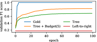
Figure 3: $F_{1}$ score for tagging ListOps nodes with their valency, using a latent tree. Incorporating inductive bias via budget constraints improves performance.

The ListOps dataset (Nangia and Bowman,, 2018) is a synthetic collection of bracketed expressions, such as [max 2 9 [min 4 7 ] 0 ]. The arguments are lists of integers, and the operators are set summarizers such as median, max, sum, etc. It was proposed as a litmus test for studying latent tree learning models, since the syntax is essential to the semantics. Instead of tackling the challenging task of learning to evaluate the expressions, we follow Corro and Titov, 2019b and study a tagging task: labeling each operator with the number of arguments it governs.

Model architecture.

We encode the sequence with a BiLSTM, yielding vectors $\bm{h}_{1},\dots,\bm{h}_{L}$. We compute the score of dependency arc $i\rightarrow j$ as the dot product between the outputs of two mappings, one for encoding the head and one for the modifier (target word):

$$\begin{gathered}\bm{f}_{\text{hd}}(\bm{h})=\bm{W}_{\text{hd}}\bm{h}+\bm{b}_{\text{hd}};\quad\bm{f}_{\text{mo}}(\bm{h})=\bm{W}_{\text{mo}}\bm{h}+\bm{b}_{\text{mo}};\\[6.0pt] \eta_{i\rightarrow j}=\langle\bm{f}_{\text{hd}}(\bm{h}_{i}),\operatorname{ReLU}(\bm{f}_{\text{mo}}(\bm{h}_{j}))\rangle.\end{gathered}$$

We perform LP-SparseMAP optimization to get the sparse arc posterior probabilities, using different factor graph structures $\mathcal{F}$, described in the next paragraph.

$$\bm{\mu}=\operatorname{LP-SparseMAP}_{\mathcal{F}}(\bm{\eta})$$ (19)

The arc posteriors $\bm{\mu}$ correspond to a sparse combination of dependency trees. We perform one iteration of a Graph Convolutional Network (GCN) along the edges in $\bm{\mu}$. Crucially, the input to the GCN is not the BiLSTM output $(\bm{h}_{1},\dots,\bm{h}_{L})$ but a “de-lexicalized” sequence $(\bm{v},\dots,\bm{v})$ where $\bm{v}$ is a learned parameter vector, repeated $L$ times regardless of the tokens. This forces the predictions to rely on the GCN and thus on the latent trees, preventing the model from using the global BiLSTM to “cheat”. The GCN produces contextualized representations $(\bm{g}_{1},\dots,\bm{g}_{L})$ which we then pass through an output layer to predict the valency label for each operator node.

Factor graphs.

Unlike Corro and Titov, 2019b , who use projective dependency parsing, we consider the general non-projective case, making the problem more challenging. The MAP oracle is the maximum arborescence algorithm (Chu and Liu,, 1965; Edmonds,, 1967).

Table 2: ListOps tagging results with non-projective latent trees. The budget constraints bring improvement.

	validation		test
	Acc.	$F_{1}$	Acc.	$F_{1}$
left-to-right	28.14	17.54	28.07	17.43
tree	68.23	68.74	68.74	69.12
tree+budget	82.35	82.59	82.75	82.95

First, we consider a factor graph with a single non-projective TREE factor: in this case, LP-SparseMAP reduces to a SparseMAP baseline. Motivated by multiple observations that SparseMAP and similar latent structure learning methods tend to learn trivial trees (Williams et al.,, 2018) we next consider overlaying constraints in the form of BUDGET factors on top of the TREE factor. For every possible head $i$, we include a BUDGET factor allowing at most five of the possible outgoing arcs $(\mu_{i\rightarrow 1},\dots,\mu_{i\rightarrow L})$ to be selected.

Results.

Figure 3 confirms that, unsurprisingly, the baseline with access to gold dependency structure quickly learns to predict perfectly, while the simple left-to-right baseline cannot progress. LP-SparseMAP with BUDGET constraints on the modifiers outperforms SparseMAP by over 10 percentage points (Table 2).

5.2 Natural language inference
with decomposable structured attention

We now turn to the task of natural language inference, using LP-SparseMAP to uncover hidden alignments for structured attention networks. Natural language inference is a pairwise classification task. Given a premise of length $m$, and a hypothesis of length $n$, the pair must be classified into one of three possible relationships: entailment, contradiction, or neutrality. We use the English language SNLI and MultiNLI datasets (Bowman et al.,, 2015; Williams et al.,, 2017), with the same preprocessing and splits as Niculae et al., (2018).

Model architecture.

We use the model of Parikh et al., (2016) with no intra-attention. The model computes a joint attention score matrix $\bm{S}$ of size $m\times n$, where $s_{ij}$ depends only on $i$th word in the premise and the $j$th word in the hypothesis (hence decomposable). For each premise word $i$, we apply softmax over the $i$^th row of $\bm{S}$ to get a weighted average of the hypothesis. Then, similarly, for each hypothesis word $j$, we apply softmax over the $j$^th row of $\bm{S}$ yielding a representation of the premise. From then on, each word embedding is combined with its corresponding weighted context using an affine function, the results are sum-pooled and passed through an output multi-layer perceptron to make a classification. We propose replacing the independent softmax attention with structured, joint attention, normalizing over both rows and columns simultaneously in several different ways, using LP-SparseMAP with scores $\eta_{ij}=s_{ij}$. We use frozen GloVe embeddings (Pennington et al.,, 2014), and all our models have 130k parameters (cf. App.  E).

Factor graphs.

Assume $m\leq n$. First, like Niculae et al., (2018), we consider a matching factor $f$:

$$\mathcal{M}_{f}\!=\!\Big{\{}\bm{\mu}\in[0,1]^{mn};\!\!\sum_{j\in[n]}\mu_{ij}=1,\sum_{i\in[m]}\mu_{ij}\leq 1\Big{\}}.$$ (20)

Table 3: NLI accuracy scores with structured attention. The LP-SparseMAP models perform competitively.

	SNLI		MultiNLI
	valid	test	valid	test
softmax	84.44	84.62	70.06	69.42
matching	84.57	84.16	70.84	70.36
LP-matching	84.70	85.04	70.57	70.64
LP-sequential	83.96	83.67	71.10	71.17

When $m=n$, linear maximization on this constraint set corresponds to the linear assignment problem, solved by the Kuhn-Munkres (Kuhn,, 1955) or Jonker-Volgenant (Jonker and Volgenant,, 1987) algorithms, and the solution is a doubly stochastic matrix. When $m<n$, the scores can be padded with $-\infty$ to a square matrix prior to invoking the algorithm. A linear maximization thus takes $\mathcal{O}(n^{3})$, and this instantiation of structured matching attention can be tackled by SparseMAP. Next we consider a relaxed equivalent formulation which we call LP-matching, as shown in Figure 2, with one XOR factor per row and one AtMostOne factor per column:

$$\mathcal{F}={} \{\textsf{XOR}(\mu_{i1},\dots,\mu_{in}):i\in[m]\}$$ (21)

$$\cup\{\textsf{AtMostOne}(\mu_{1j},\dots,\mu_{mj}):j\in[n]\}$$

Each subproblem can be solved in $\mathcal{O}(n)$ for a total complexity of $\mathcal{O}(n^{2})$ per iteration (cf. Appendix D). While more iterations may be necessary to converge, the finer-grained approach might make faster progress, yielding more useful latent alignments. Finally, we consider a more expressive joint alignment that encourages continuity. Inspired by the sequential alignment of Niculae et al., (2018), we propose a bi-directional model called LP-sequence, consisting of a coarse, linear-chain Markov factor (with MAP provided by the Viterbi algorithm; Rabiner,, 1989) parametrized by a single transition score $\eta_{N}$ for every pair of alignments $(i,j)-(i+1,j\pm 1)$. By itself, this factor may align multiple premise words to the same hypothesis word. We symmetrize it by overlaying $m$ AtMostOne factors, like in Eq.  21, ensuring each hypothesis word is aligned on average to at most one premise word. Effectively, this results in a sequence tagger constrained to use each of the $m$ states at most once. For both LP-SparseMAP approaches, we rescale the result by row sums to ensure feasibility.

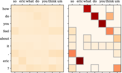
Figure 4: Attention induced using softmax (left) and LP-SparseMAP sequential (right) on a MultiNLI example. With this inductive bias, LP-SparseMAP learns a bi-directional alignment anchoring longer phrases.

Results.

Table 3 reveals that LP-matching is the best performing mechanism on SNLI, and LP-sequential on MultiNLI. The $\eta_{N}$ transition score learned by LP-sequential is 1.6 on SNLI and 2.5 on MultiNLI, and Figure 4 shows an example of the useful inductive bias it learns. On both datasets, the relaxed LP-matching outperforms the coarse matching factor, suggesting that, indeed, equivalent parametrizations of a model may perform differently when not run until convergence.

Table 4: Multilabel classification test $F_{1}$ scores.

	bibtex	bookmarks
Unstructured	42.28	35.76
Structured hinge loss	37.70	33.26
LP-SparseMAP loss	43.43	36.07

5.3 Multilabel classification

Finally, to confirm that LP-SparseMAP is also suitable as in the supervised setting, we evaluate on the task of multilabel classification. Our factor graph has $k$ binary variables (one for each label), and a pairwise factor for every label pair:

$$\mathcal{F}=\{\textsf{PAIR}(\mu_{i},\mu_{j};\eta_{ij}):1\leq i<j\leq k\}.$$ (22)

This yields the standard fully-connected pairwise MRF:

$$\langle\bm{\eta},\bm{\mu}\rangle=\sum_{i}\mu_{i}\eta_{i}+\sum_{i<j}\mu_{i}\mu_{j}\eta_{ij}.$$ (23)

Neural network parametrization.

We use a 2-layer multi-layer perceptron to compute the score for each variable. In the structured models, we have an additional $\nicefrac{{1}}{{2}}~{}k(k-1)$ parameters for the co-occurrence score of every pair of classes. We compare an unstructured baseline (using the binary logistic loss for each label), a structured hinge loss (with LP-MAP inference) and a LP-SparseMAP loss model. We solve LP-MAP using AD³ and LP-SparseMAP with our proposed algorithm (cf. Appendix E).

Results.

Table 4 shows the example $F_{1}$ score on the test set for the bibtex and bookmarks benchmark datasets (Katakis et al.,, 2008). The structured hinge loss model is worse than the unstructured (binary logistic loss) baseline; the LP-SparseMAP loss model outperforms both. This suggests that the LP-SparseMAP loss is promising for structured output learning. We note that, in strictly-supervised setting, approaches that blend inference with learning (e. g., Chen et al.,, 2015; Tang et al.,, 2016) may be more efficient; however, LP-SparseMAP can work both as a hidden layer and a loss, with no redundant computation.

6 Related work

Differentiable optimization.

The most related research direction involves bi-level optimization, or argmin differentiation (Gould et al.,, 2016; Djolonga and Krause,, 2017); Typically, such research assumes problems are expressible in a standard form, for instance using quadratic programs (Amos and Kolter,, 2017) or generic disciplined convex programs (Section 7, Amos,, 2019; Agrawal et al., 2019a, ; Agrawal et al., 2019b, ). We take inspiration from this line of work by developping LP-SparseMAP as a flexible domain-specific language for defining latent structure. The generic approaches are not applicable for the typical optimization problems arising in structured prediction, because of the intractably large number of constraints typically necessary, and the difficulty of formulating many problems in standard forms. Our method instead assumes interacting through the problem through local oracle algorithms, exploiting the structure of the factor graph and allowing for more efficient handling of coarse factors and logic constraints via nested subproblems.

Latent structure models.

Our motivation and applications are mostly focused on learning with latent structure. Specifically, we are interested in global optimization methods, which require marginal inference or similar relaxations (Kim et al.,, 2017; Liu and Lapata,, 2018; Corro and Titov, 2019a, ; Corro and Titov, 2019b, ; Niculae et al.,, 2018), rather than incremental methods based on policy gradients (Yogatama et al.,, 2017). Promising methods exist for approximate marginal inference in factor graphs with MAP calls (Belanger et al.,, 2013; Krishnan et al.,, 2015; Tang et al.,, 2016), relying on entropy approximation penalties. Such approaches focus on supervised structure prediction, which is not our main goal; and their backward passes has not been studied to our knowledge. Importantly, as these penalties are non-quadratic, the active set algorithm does not apply, falling back to the more general variants of Frank-Wolfe. The active set algorithm is a key ingredient of our work, as it exhibits fast finite convergence, finds sparse solutions and – crucially – provides precomputation of the matrix inverse required in the backward pass (Niculae et al.,, 2018). In contrast, the quadratic penalty (Meshi et al.,, 2015; Niculae et al.,, 2018) is more amenable to optimization, as well as bringing other sparsity benefits. The projection step of Peng et al., (2018) can be cast as a SparseMAP problem, thus our algorithm can be used to also extend their method to arbitrary factor graphs. For pairwise MRFs (a class of factor graphs), differentiating belief propagation, either through unrolling or perturbation-based approximation, has been studied (Stoyanov et al.,, 2011; Domke,, 2013). Our approach instead computes implicit gradients, which is more efficient, thanks to quantities precomputed in the forward pass, and in some circumstances has been shown to work better (Rajeswaran et al.,, 2019). Finally, MRF-based approaches have not been explored in the presence of logic constraints or coarse factors, while our formulation is built from the beginning with such use cases in mind.

7 Conclusions

We introduced LP-SparseMAP, an extension of SparseMAP to sparse differentiable optimization in any factor graph, enabling neural hidden layers with arbitrarily complex structure, specified using a familiar domain-specific language. We have shown LP-SparseMAP to outperform SparseMAP for latent structure learning, and outperform the structured hinge for structured output learning. We hope that our toolkit empowers future research on latent structure, leading to powerful models based on domain knowledge. In future work, we shall investigate further applications where expertise about the domain structure, together with minimal self-supervision deployed via the LP-SparseMAP loss, may lead to data-efficient learning, even for more expressive models without artificial bottlenecks.

Appendix A Separable reformulation of LP-SparseMAP

Lemma 1.

Let $\bm{\delta}$, $\bm{D}$, $\widetilde{\bm{C}}$, $\widetilde{\bm{M}}$ defined as in Proposition 1. Let $\bm{S}=\operatorname{diag}(\bm{\delta})$. Then,

1. $\bm{C}^{\top}\bm{C}=\bm{S}^{2}$

2. $\widetilde{\bm{C}}=\bm{C}\bm{S}^{-1}$;

3. $\widetilde{\bm{C}}^{\top}\widetilde{\bm{C}}=\bm{I}$;

4. For any feasible pair $(\bm{\mu},\bm{p})$, $\bm{\mu}=\widetilde{\bm{C}}^{\top}\widetilde{\bm{M}}\bm{p}$, and $\|\bm{\mu}\|=\|\widetilde{\bm{M}}\bm{p}\|.$

Proof.

(i) The matrix $\bm{C}$, which expresses the agreement constraint $\bm{C}\bm{\mu}=\bm{M}\bm{p}$, is a stack of selector matrices, in other words, its sub-blocks are either the identity $\bm{I}$ or the zero matrix $\bm{0}$. We index its rows by pairs $(f,k):f\in\mathcal{F},k\in[d_{f}]$, and its columns by $j\in[d]$. Denote by $f_{(k)}=j$ the fact that the $k$^th variable under factor $f$ is $\bm{\mu}_{j}$. Then, $(\bm{C})_{(f,k),j}=\llbracket f_{(k)}=j\rrbracket$. We can then explicitly compute

$$(\bm{C}^{\top}\bm{C})_{ij}=\sum_{f\in\mathcal{F}}\sum_{k\in[d_{f}]}\llbracket f_{(k)}=i\rrbracket\llbracket f_{(k)}=j\rrbracket.$$

If $i\neq j$, $\llbracket f_{(k)}=i\rrbracket\llbracket f_{(k)}=j\rrbracket=0$, so $(\bm{C}^{\top}\bm{C})_{ij}=\begin{cases}\deg(j)&i=j,\\ 0,&\text{o.w.}\end{cases}=\bm{S}^{2}$.

(ii) By construction, $\bm{D}_{(f,k),(f,k)}=(\bm{C}\bm{\delta})_{(f,k)}=\sum_{i\in[d]}\llbracket f_{(k)}=i\rrbracket\sqrt{\deg(i)}=\sqrt{\deg(j)},$ for the unique variable $j$ with $f_{(k)}=j$. Thus,

$$(\bm{D}^{-1}\bm{C})_{(f,k),j}=\llbracket f_{(k)}=j\rrbracket\sqrt{\deg(j)}=(\bm{C}\bm{S}^{-1})_{(f,k),j}.$$

(iii) It follows from (i) and (ii) that $\widetilde{\bm{C}}^{\top}\widetilde{\bm{C}}=\bm{S}^{-1}\bm{C}^{\top}\bm{C}\bm{S}^{-1}=\bm{S}^{-1}\bm{S}^{2}\bm{S}^{-1}=\bm{I}$.

(iv) Since $\bm{D}$ is full-rank, the feasibility condition is equivalent to $\widetilde{\bm{C}}\bm{\mu}=\widetilde{\bm{M}}\bm{p}$. Left-multiplying by $\widetilde{\bm{C}}^{\top}$ yields $\bm{\mu}=\widetilde{\bm{C}}^{\top}\widetilde{\bm{M}}\bm{p}$. Moreover, $\|\widetilde{\bm{M}}\bm{p}\|^{2}=\|\widetilde{\bm{C}}\bm{\mu}\|^{2}=\bm{\mu}^{\top}\widetilde{\bm{C}}^{\top}\widetilde{\bm{C}}\bm{\mu}=\|\bm{\mu}\|^{2}.$ ∎

Appendix B Derivation of updates and comparison to LP-MAP

Recall the problem we are trying to minimize, from Eq.  11:

$$\underset{\bm{\mu},~{}\bm{p}}{\text{maximize}}\sum_{f\in\mathcal{F}}\langle\bm{\eta}_{f},\bm{A}_{f}\bm{p}_{f}\rangle-.5\|\widetilde{\bm{M}}_{f}\bm{p}_{f}\|^{2}~{}~{}~{}\text{subject to}~{}~{}~{}\bm{p}\in\triangle_{f_{1}}\times\triangle_{f_{2}}\times\dots\times\triangle_{f_{n}},~{}\widetilde{\bm{C}}\bm{\mu}=\widetilde{\bm{M}}\bm{p}.$$ (24)

Since the simplex constraints are separable, we may move them to the objective, yielding

$$\underset{\bm{\mu},~{}\bm{p}}{\text{maximize}}~{}~{}\sum_{f\in\mathcal{F}}\langle\bm{\eta}_{f},\bm{A}_{f}\bm{p}_{f}\rangle-.5\|\widetilde{\bm{M}}_{f}\bm{p}_{f}\|^{2}-\iota_{\triangle_{f}}(\bm{p}_{f})\quad\text{subject to}\quad~{}\widetilde{\bm{C}}\bm{\mu}=\widetilde{\bm{M}}\bm{p}.$$ (25)

The $\gamma$-augmented Lagrangian of problem 25 is

$$\mathcal{L}_{\gamma}(\bm{\mu},\bm{p}.\bm{\lambda}) =\sum_{f\in\mathcal{F}}\Big{(}\langle\bm{\eta}_{f},\bm{A}_{f}\bm{p}_{f}\rangle-.5\|\widetilde{\bm{M}}_{f}\bm{p}_{f}\|^{2}-\iota_{\triangle_{f}}(\bm{p}_{f})\Big{)}-\langle\bm{\lambda},\widetilde{\bm{C}}\bm{\mu}-\widetilde{\bm{M}}\bm{p}\rangle-\frac{\gamma}{2}\|\widetilde{\bm{C}}\bm{\mu}-\widetilde{\bm{M}}\bm{p}\|^{2}.$$ (26)

The solution $\bm{\mu}^{\star},\bm{p}^{\star},\bm{\lambda}^{\star}$ is a saddle point of the Lagrangian, i. e., a solution of

$$\min_{\bm{\lambda}}\max_{\bm{p},\bm{\mu}}\mathcal{L}_{\gamma}(\bm{\mu},\bm{p},\bm{\lambda})$$ (27)

ADMM optimizes Eq.  27 in a block-coordinate fashion; we next derive each block update.

B.1 Updating $p$

We update $\bm{p}_{f}$ for each $f\in\mathcal{F}$ independently by solving:

$$\bm{p}_{f}^{(t)}\leftarrow\operatorname*{arg\,max}_{\bm{p}_{f}}{} \mathcal{L}_{\gamma}(\bm{\mu}^{(t-1)},\bm{p},\bm{\lambda}^{(t-1)})$$ (28)

Denoting $\bm{\eta}_{f}=[\bm{\eta}_{f,M},\bm{\eta}_{f,N}]$, we have that

$$\langle\bm{\eta}_{f},\bm{A}_{f}\bm{p}_{f}\rangle=\langle\bm{\eta}_{f,M},\bm{M}_{f}\bm{p}_{f}\rangle+\langle\bm{\eta}_{f,N},\bm{N}_{f}\bm{p}_{f}\rangle=\langle\bm{D}_{f}\bm{\eta}_{f,M},\widetilde{\bm{M}}_{f}\bm{p}_{f}\rangle+\langle\bm{\eta}_{f,N},\bm{N}_{f}\bm{p}_{f}\rangle$$

The $\gamma$-augmented term regularizing the subproblems toward the current estimate of the global solution $\bm{\mu}^{(t-1)}$ is

$$\frac{\gamma}{2}\|\widetilde{\bm{C}}_{f}\bm{\mu}^{(t-1)}-\widetilde{\bm{M}}_{f}\bm{p}_{f}\|^{2}=\frac{\gamma}{2}\|\widetilde{\bm{M}}_{f}\bm{p}_{f}\|-\gamma\langle\widetilde{\bm{C}}_{f}\bm{\mu}^{(t-1)},\widetilde{\bm{M}}_{f}\bm{p}_{f}\rangle+\text{const}$$

For each factor, the subproblem objective is therefore:

$$f(\bm{p}_{f}) =\langle\bm{\eta}_{f},\bm{A}_{f}\bm{p}_{f}\rangle-\langle\bm{\lambda}^{(t)}_{f},\widetilde{\bm{M}}_{f}\bm{p}_{f}\rangle-\frac{\gamma}{2}\|\widetilde{\bm{C}}_{f}\bm{\mu}^{(t-1)}-\widetilde{\bm{M}}_{f}\bm{p}\|^{2}-\frac{1}{2}\|\widetilde{\bm{M}}_{f}\bm{p}\|^{2}$$ (29)

$$=\langle\bm{D}_{f}\bm{\eta}_{f,M}-\bm{\lambda}^{(t-1)}_{f}+\gamma\widetilde{\bm{C}}_{f}\bm{\mu}^{(t-1)},\widetilde{\bm{M}}_{f}\bm{p}_{f}\rangle+\langle\bm{\eta}_{f,N},\bm{N}_{f}\bm{p}_{f}\rangle-\frac{1+\gamma}{2}\|\widetilde{\bm{M}}_{f}\bm{p}_{f}\|^{2}+\text{const}$$

$$\propto\langle\widetilde{\bm{\eta}}_{f,M},\widetilde{\bm{M}}_{f}\bm{p}_{f}\rangle+\langle\widetilde{\bm{\eta}}_{f,N},\bm{N}_{f}\bm{p}_{f}\rangle-\frac{1}{2}\|\widetilde{\bm{M}}_{f}\bm{p}_{f}\|^{2}+\text{const}.$$

This is exactly a SparseMAP instance with $\widetilde{\bm{\eta}}_{f,M}=\frac{1}{1+\gamma}\big{(}\bm{D}_{f}\bm{\eta}_{f,M}-\bm{\lambda}^{(t-1)}_{f}+\gamma\widetilde{\bm{C}}_{f}\bm{\mu}^{(t-1)}\big{)}$ and $\widetilde{\bm{\eta}}_{f,N}=\frac{1}{1+\gamma}\bm{\eta}_{f,N}$.

Observation. For comparison, when solving LP-MAP with AD³, the subproblems minimize the objective

$$f(\bm{p}_{f}) =\langle\bm{\eta}_{f},\bm{A}_{f}\bm{p}_{f}\rangle-\langle\bm{\lambda}^{(t)}_{f},\bm{M}_{f}\bm{p}_{f}\rangle-\frac{\gamma}{2}\|\bm{C}_{f}\bm{\mu}^{(t)}-\bm{M}_{f}\bm{p}_{f}\|^{2}$$ (30)

$$=\langle\bm{\eta}_{f,M}-\bm{\lambda}^{(t)}_{f}+\gamma\bm{C}_{f}\bm{\mu}^{(t)},\bm{M}_{f}\bm{p}_{f}\rangle+\langle\bm{\eta}_{f,N},\bm{N}_{f}\bm{p}_{f}\rangle-\frac{\gamma}{2}\|\bm{M}_{f}\bm{p}_{f}\|^{2},$$

so the $\bm{p}$-update is a SparseMAP instance with $\widetilde{\bm{\eta}}_{f,M}=\frac{1}{\gamma}\big{(}\bm{\eta}_{f,M}-\bm{\lambda}^{(t)}_{f}+\gamma\bm{C}_{f}\bm{\mu}^{(t)}\big{)}$ and $\widetilde{\bm{\eta}}_{f,N}=\frac{1}{\gamma}\bm{\eta}_{f,N}$. Notable differences is the scaling by $1+\gamma$ instead of $\gamma$ (corresponding to the added regularization), and the diagonal degree reweighting.

B.2 Updating $\mu$

We must solve

$$\bm{\mu}^{(t)} \leftarrow\operatorname*{arg\,max}_{\bm{\mu}}~{}\mathcal{L}_{\gamma}(\bm{\mu},\bm{p}^{(t)},\bm{\lambda}^{(t-1)})$$ (31)

$$=\operatorname*{arg\,min}_{\bm{\mu}}~{}\frac{\gamma}{2}\|\widetilde{\bm{C}}\bm{\mu}-\widetilde{\bm{M}}\bm{p}^{(t)}\|^{2}+\langle\widetilde{\bm{C}}^{\top}\bm{\lambda}^{(t-1)},\bm{\mu}\rangle.$$

This is an unconstrained problem. Setting the gradient of the objective to $\bm{0}$, we get

$$\bm{0} \stackrel{{\scriptstyle!}}{{=}}\gamma\widetilde{\bm{C}}^{\top}(\widetilde{\bm{C}}\bm{\mu}-\widetilde{\bm{M}}\bm{p}^{(t)})+\widetilde{\bm{C}}^{\top}\bm{\lambda}^{(t-1)}$$ (32)

$$=\gamma(\bm{\mu}-\widetilde{\bm{C}}^{\top}\widetilde{\bm{M}}\bm{p}^{(t)})+\widetilde{\bm{C}}^{\top}\bm{\lambda}^{(t-1)}$$

with the unique solution

$$\mu^{(t)} \leftarrow\widetilde{\bm{C}}\widetilde{\bm{M}}\bm{p}^{(t)}-\frac{1}{\gamma}\widetilde{\bm{C}}^{\top}\bm{\lambda}^{(t-1)}$$ (33)

$$=\widetilde{\bm{C}}\widetilde{\bm{M}}\bm{p}^{(t)},$$ (34)

where the last step follows from the fact that our resulting algorithm maintains the invariant $\widetilde{\bm{C}}^{\top}\bm{\lambda}^{(\cdot)}=0$, as we show in the next section.

B.3 Updating the Lagrange multipliers

Since $\mathcal{L}_{\gamma}$ is linear in $\bm{\lambda}$, $\min_{\bm{\lambda}}\mathcal{L}_{\gamma}(\bm{\lambda})=-\infty$, therefore we may not globally minimize w. r. t. $\bm{\lambda}$. Instead, we make only a small gradient step:

$$\bm{\lambda}^{(t)}\leftarrow\bm{\lambda}^{(t-1)}+\gamma\big{(}\widetilde{\bm{C}}\bm{\mu}^{(t)}-\widetilde{\bm{M}}\bm{p}^{(t)}\big{)}.$$ (35)

As promised, we inspect below the value of $\widetilde{\bm{C}}^{\top}\bm{\lambda}$ under this update rule.

$$\widetilde{\bm{C}}^{\top}\bm{\lambda}^{(t)} =\widetilde{\bm{C}}^{\top}\bm{\lambda}^{(t-1)}+\gamma(\cancel{\widetilde{\bm{C}}}^{\top}\cancel{\widetilde{\bm{C}}}\bm{\mu}^{(t)}-\widetilde{\bm{C}}^{\top}\widetilde{\bm{M}}\bm{p}^{t})$$ (36)

$$=\widetilde{\bm{C}}^{\top}\bm{\lambda}^{(t-1)}+\gamma\big{(}\bm{\mu}^{(t)}-(\bm{\mu}^{(t)}+\frac{1}{\gamma}\widetilde{\bm{C}}^{\top}\bm{\lambda}^{(t-1)})\big{)}\quad\text{(from Eq.~{}\ref{eqn:mu_update_orig})}$$

$$=\widetilde{\bm{C}}^{\top}\bm{\lambda}^{(t-1)}-\frac{\gamma}{\gamma}\widetilde{\bm{C}}^{\top}\bm{\lambda}^{(t-1)}=0.$$

Appendix C Backward pass

C.1 SparseMAP

As a reminder, we repeat here the form of the SparseMAP Jacobian (Niculae et al.,, 2018), along with a brief derivation. This result plays an important role in LP-SparseMAP backward pass.

Proposition 4.

Given a structured problem with $\bm{A}=[\bm{M},\bm{N}]$, denote the SparseMAP solution for input scores $\bm{\eta}=[\bm{\eta}_{M},\bm{\eta}_{N}]$ as $\bm{\mu}$ where

$$(\bm{\mu},\bm{p})=\operatorname*{arg\,max}_{\begin{subarray}{c}\bm{\mu}=\bm{M}\bm{p}\\ \bm{p}\in\triangle\end{subarray}}\langle\bm{\eta},\bm{A}\bm{p}\rangle-\frac{1}{2}\|\bm{\mu}\|^{2}.$$ (37)

Let $\mathcal{S}=\{y_{1},\dots,y_{k}\}\subset\mathcal{Y}$ denote the support set of selected structures, and denote $\bar{\bm{M}}\coloneqq\bm{M}_{\mathcal{S}}\in\mathbb{R}^{d_{M}\times|\mathcal{S}|}$, $\bar{\bm{N}}\coloneqq\bm{N}_{\mathcal{S}}\in\mathbb{R}^{d_{N}\times|\mathcal{S}|}$, and

$$\bm{Z}=(\bar{\bm{M}}^{\top}\bar{\bm{M}})^{-1},\quad\bm{z}=\bm{Z}\bm{1},\quad\bm{Q}=\bm{Z}-\frac{\bm{z}\bm{z}^{\top}}{\bm{1}^{\top}\bm{z}}.$$ (38)

Then, we have

$$\frac{\partial\bm{\mu}}{\partial\bm{\eta}_{M}}(\bm{\eta}_{M},\bm{\eta}_{N})=\bar{\bm{M}}\bm{Q}\bar{\bm{M}}^{\top},\qquad\frac{\partial\bm{\mu}}{\partial\bm{\eta}_{N}}(\bm{\eta}_{M},\bm{\eta}_{N})=\bar{\bm{M}}\bm{Q}\bar{\bm{N}}.$$ (39)

Proof.

Rewrite the optimization problem in Eq. 37 in terms of a convex combination of structures:

$$\text{minimize}~{}\langle\bm{\theta},\bm{p}\rangle-\frac{1}{2}\|\bm{M}\bm{p}\|^{2}\quad\text{subject to}~{}\bm{p}\in\triangle.$$ (40)

The Lagrangian is given by

$$\mathcal{L}(\bm{p},\bm{\nu},\tau)=\frac{1}{2}\|\bm{M}\bm{p}\|^{2}-\langle\bm{\theta}-\tau\bm{1}-\bm{\nu},\bm{p}\rangle.$$ (41)

The solution $\bm{p}$ is sparse with nonzero coordinates $\mathcal{S}$. Small changes to $\bm{\theta}$ only lead to changes in $\mathcal{S}$ on a measure-zero set of critical tie-breaking points, and there is always a direction of change that leaves $\mathcal{S}$ unchanged. We may thus assume that $\mathcal{S}$ does not change with small changes to $\bm{\theta}$, yielding the Jacobian at most points, and a generalized Jacobian otherwise (Clarke,, 1990).

From complementary slackness, $\bar{\bm{\nu}}=\bm{0}$, so the conditions $\nabla_{\bar{\bm{p}}}\mathcal{L}\stackrel{{\scriptstyle!}}{{=}}\bm{0}$ and $\bm{1}^{\top}\bar{\bm{p}}\stackrel{{\scriptstyle!}}{{=}}1$ can be written as

$$\begin{bmatrix}\bar{\bm{M}}^{\top}\bar{\bm{M}}&\bm{1}\\ \bm{1}^{\top}&0\\ \end{bmatrix}~{}\begin{bmatrix}\bar{\bm{p}}\\ \tau\\ \end{bmatrix}~{}=~{}\begin{bmatrix}\bar{\bm{\theta}}\\ 1\\ \end{bmatrix}.$$ (42)

Therefore, differentiating w.r.t. $\bar{\bm{\theta}}$, the Jacobians $\frac{\partial\bar{\bm{p}}}{\partial\bar{\bm{\theta}}}$ and $\frac{\partial\tau}{\partial\bar{\bm{\theta}}}$ must satisfy

$$\begin{bmatrix}\bar{\bm{M}}^{\top}\bar{\bm{M}}&\bm{1}\\ \bm{1}^{\top}&0\\ \end{bmatrix}~{}\begin{bmatrix}\frac{\partial\bar{\bm{p}}}{\partial\bar{\bm{\theta}}}\\ \frac{\partial\tau}{\partial\bar{\bm{\theta}}}\\ \end{bmatrix}~{}=~{}\begin{bmatrix}\bm{I}\\ 0\\ \end{bmatrix}.$$ (43)

Denote by $\bm{Z}\coloneqq(\bar{\bm{M}}^{\top}\bar{\bm{M}})^{-1},\bm{z}=\bm{Z}\bm{1},t\coloneqq\bm{1}^{\top}\bm{z},\bm{Q}=\bm{Z}-\frac{\bm{zz}^{\top}}{t}.$ Using block-matrix inversion,

$$\begin{bmatrix}\bar{\bm{M}}^{\top}\bar{\bm{M}}&\bm{1}\\ \bm{1}^{\top}&0\\ \end{bmatrix}^{-1}=\begin{bmatrix}\bm{Q}&\nicefrac{{\bm{z}}}{{t}}\\ \nicefrac{{\bm{z}^{\top}}}{{t}}&-\nicefrac{{1}}{{t}}\\ \end{bmatrix}.$$ (44)

Therefore, $\frac{\partial\bar{\bm{p}}}{\partial\bar{\bm{\theta}}}=\bm{Q}$. Since $\bm{\mu}_{M}=\bar{\bm{M}}{\bar{\bm{p}}}$ and $\bar{\bm{\theta}}=\bar{\bm{M}}^{\top}\bm{\eta}_{M}+\bar{\bm{N}}^{\top}\bm{\eta}_{N}$, the chain rule gives Eq. 39. Importantly, when using the active set method for computing the SparseMAP solution (Niculae et al.,, 2018), the inverse in Eq. 44, and thus $\bm{Q}$, is precomputed incrementally during the forward pass, and thus readily available for no extra cost..

∎

C.2 LP-SparseMAP

Proof.

Given variable scores $\bm{\eta}_{M}$ and factor scores $\bm{\eta}_{f,N}$, we construct a vector $\bm{\theta}=\bar{\bm{M}}^{\top}\widetilde{\bm{C}}\bm{\eta}_{M}+\bm{N}\bm{\eta}_{f,N}$. To derive the backward pass, we start from the Lagrangian with simplex constraints:

$$\mathcal{L}(\bm{\mu},\bm{p}.\bm{\lambda}.\bm{\tau},\bm{\nu})=\langle\bm{\theta},\bm{p}\rangle-\frac{1}{2}\|\widetilde{\bm{M}}\bm{p}\|^{2}-\langle\bm{\lambda},\widetilde{\bm{C}}\bm{\mu}-\widetilde{\bm{M}}\bm{p}\rangle-\langle\bm{\tau},\bm{B}\bm{p}-\bm{1}\rangle-\langle\bm{\nu},\bm{p}\rangle.$$ (45)

where $\bm{B}$ is a matrix with row-vectors $\bm{1}$ along the diagonal (so that $\bm{B}\bm{p}=[\cdots,\bm{1}\bm{p}_{f},\cdots]$). For any feasible $(\bm{p},\bm{\mu})$ we have that $\|\widetilde{\bm{M}}\bm{p}\|^{2}=\|\bm{\mu}\|^{2}$, so we may rewrite the Lagrangian as:

$$\mathcal{L}(\bm{\mu},\bm{p}.\bm{\lambda}.\bm{\tau},\bm{\nu})=\langle\bm{\theta},\bm{p}\rangle-\frac{1}{4}\|\widetilde{\bm{M}}\bm{p}\|^{2}-\frac{1}{4}\|\bm{\mu}\|^{2}-\langle\bm{\lambda},\widetilde{\bm{C}}\bm{\mu}-\widetilde{\bm{M}}\bm{p}\rangle-\langle\bm{\tau},\bm{B}\bm{p}-\bm{1}\rangle-\langle\bm{\nu},\bm{p}\rangle.$$ (46)

The corresponding optimality conditions are

$$\bm{0}\stackrel{{\scriptstyle!}}{{=}}\nabla_{\bm{p}_{f}}\mathcal{L} =\bm{\theta}-.5\widetilde{\bm{M}}_{f}^{\top}\widetilde{\bm{M}}_{f}\bm{p}_{f}+\widetilde{\bm{M}}_{f}^{\top}\bm{\lambda}_{f}-\tau_{f}\bm{1}-\bm{\nu}_{f}\quad\text{for all}~{}f\in\mathcal{F},$$ (47)

$$\bm{0}\stackrel{{\scriptstyle!}}{{=}}\nabla_{\bm{\mu}}\mathcal{L} =-.5\bm{\mu}-\widetilde{\bm{C}}^{\top}\bm{\lambda}$$ (48)

$$\bm{0}\stackrel{{\scriptstyle!}}{{=}}\nabla_{\bm{\lambda}}\mathcal{L} =\widetilde{\bm{C}}\bm{\mu}-\widetilde{\bm{M}}\bm{p}$$ (49)

$$\bm{0}\stackrel{{\scriptstyle!}}{{=}}\nabla_{\bm{\tau}}\mathcal{L} =\bm{B}\bm{p}-\bm{1}$$ (50)

along with $\bm{\nu}\geq 0,\bm{p}\geq 0,$ and the complementarity slackness conditions $\langle\bm{\nu},\bm{p}\rangle=\bm{0}$. As in App.  C.1, we observe that the support $\mathcal{S}_{f}$ of each factor $f$ does not change with small changes to $\bm{\eta}$. Once again, we use the overbar $\bar{\cdot}$ to denote the restriction of a vector or matrix to the (block-wise) support $\mathcal{S}_{f}$, resulting in, for instance,

$$\bar{\bm{p}}>0\in\mathbb{R}^{\sum_{f}|\mathcal{S}_{f}|},\quad\bar{\bm{M}}\in\mathbb{R}^{\left(\sum_{f}d_{f}\right)~{}\times~{}\left(\sum_{f}|\mathcal{S}_{f}|\right)},\quad\text{etc.}$$

On the support, $\bar{\bm{\nu}}_{f}$ vanishes, so we rewrite the conditions in terms of $\bar{\bm{p}}$. In matrix form,

$$\begin{bmatrix}.5\bar{\bm{M}}^{\top}\bar{\bm{M}}&\bar{\bm{B}}^{\top}&\bm{0}&-\bar{\bm{M}}^{\top}\\ \bar{\bm{B}}&\bm{0}&\bm{0}&\bm{0}\\ \bm{0}&\bm{0}&.5\bm{I}&\widetilde{\bm{C}}^{\top}\\ -\bar{\bm{M}}&\bm{0}&\widetilde{\bm{C}}&\bm{0}\\ \end{bmatrix}\left[\begin{array}[]{c}\bar{\bm{p}}\\ \bm{\tau}\\ \bm{\mu}\\ \bm{\lambda}\end{array}\right]=\left[\begin{array}[]{c}\bar{\bm{\theta}}\\ \bm{1}\\ \bm{0}\\ \bm{0}\end{array}\right]$$ (51)

Differentiating w.r.t. $\bar{\bm{\theta}}$ yields

$$\begin{bmatrix}.5\bar{\bm{M}}^{\top}\bar{\bm{M}}&\bar{\bm{B}}^{\top}&\bm{0}&-\bar{\bm{M}}^{\top}\\ \bar{\bm{B}}&\bm{0}&\bm{0}&\bm{0}\\ \bm{0}&\bm{0}&.5\bm{I}&\widetilde{\bm{C}}^{\top}\\ -\bar{\bm{M}}&\bm{0}&\widetilde{\bm{C}}&\bm{0}\\ \end{bmatrix}\left[\begin{array}[]{c}\bm{J}_{\bar{\bm{p}}}\\ \bm{J}_{\bm{\tau}}\\ \bm{J}_{\bm{\mu}}\\ \bm{J}_{\bm{\lambda}}\end{array}\right]=\left[\begin{array}[]{c}\bm{I}\\ \bm{0}\\ \bm{0}\\ \bm{0}\end{array}\right]$$ (52)

Observe that the top-left block can be re-organized into a block-diagonal matrix with blocks with known inverses (similar to Eq. 44)

$$\begin{bmatrix}.5\bar{\bm{M}}_{f}^{\top}\bar{\bm{M}}_{f}&\bm{1}\\ \bm{1}^{\top}&0\\ \end{bmatrix}^{-1}=\begin{bmatrix}2\bm{Q}_{f}&\cdot\\ \cdot&\cdot\\ \end{bmatrix}$$ (53)

where the values except for the top-left block can be easily obtained in terms of the blocks of Eq. 44, but this is not necessary, since all others rows and columns corresponding to $\bm{\tau}$ are zero.

We multiply the top half of the system by this inverse and eliminate $\bm{\tau}$, leaving

$$\begin{bmatrix}\bm{I}&\bm{0}&-2\bm{Q}\bar{\bm{M}}^{\top}\\ \bm{0}&.5\bm{I}&\widetilde{\bm{C}}^{\top}\\ -\bar{\bm{M}}&\widetilde{\bm{C}}&\bm{0}\\ \end{bmatrix}\left[\begin{array}[]{c}\bm{J}_{\bar{\bm{p}}}\\ \bm{J}_{\bm{\mu}}\\ \bm{J}_{\bm{\lambda}}\end{array}\right]=\left[\begin{array}[]{c}2\bm{Q}\\ \bm{0}\\ \bm{0}\end{array}\right].$$ (54)

Multiplying the first row of blocks by $\bar{\bm{M}}$, the second by $-2\bm{C}$, gives

$$\begin{bmatrix}\bar{\bm{M}}&\bm{0}&-2\bar{\bm{M}}\bm{Q}\bar{\bm{M}}^{\top}\\ \bm{0}&-\widetilde{\bm{C}}&-2\widetilde{\bm{C}}\widetilde{\bm{C}}^{\top}\\ -\bar{\bm{M}}&\widetilde{\bm{C}}&\bm{0}\\ \end{bmatrix}\left[\begin{array}[]{c}\bm{J}_{\bar{\bm{p}}}\\ \bm{J}_{\bm{\mu}}\\ \bm{J}_{\bm{\lambda}}\end{array}\right]=\left[\begin{array}[]{c}2\bar{\bm{M}}\bm{Q}\\ \bm{0}\\ \bm{0}\end{array}\right].$$ (55)

Finally, we may add up all rows to reach the expression

$$\bm{J}_{\bm{\lambda}}=-\left(\bar{\bm{M}}\bm{Q}\bar{\bm{M}}^{\top}+\widetilde{\bm{C}}\widetilde{\bm{C}}^{\top}\right)^{+}\bar{\bm{M}}\bm{Q}.$$

and, since $\bm{J}_{\bm{\mu}}=-2\widetilde{\bm{C}}^{\top}\bm{J}_{\bm{\lambda}}$, then

$$\bm{J}_{\bm{\mu}}=2\widetilde{\bm{C}}^{\top}\left(\bar{\bm{M}}\bm{Q}\bar{\bm{M}}^{\top}+\widetilde{\bm{C}}\widetilde{\bm{C}}^{\top}\right)^{+}\bar{\bm{M}}\bm{Q}.$$

The Jacobians we have been solving for so far are w.r.t. $\bm{\eta}$. We first apply the chain rule to get the Jacobian w.r.t. $\bm{\theta}_{M}$, giving

$$\frac{\partial\bm{\mu}}{\partial\bm{\eta}_{M}} =\bm{J}_{\bm{\mu}}\bar{\bm{M}}^{\top}\widetilde{\bm{C}}$$ (56)

$$=2\widetilde{\bm{C}}^{\top}\left(\bar{\bm{M}}\bm{Q}\bar{\bm{M}}^{\top}+\widetilde{\bm{C}}\widetilde{\bm{C}}^{\top}\right)^{+}\bar{\bm{M}}\bm{Q}\bar{\bm{M}}^{\top}\widetilde{\bm{C}}$$

$$=2\widetilde{\bm{C}}^{\top}\left(\bm{J}_{M}+\widetilde{\bm{C}}\widetilde{\bm{C}}^{\top}\right)^{+}\bm{J}_{M}\widetilde{\bm{C}},$$

where $\bm{J}_{M}$ is the block-wise Jacobian of each SparseMAP subproblem.

Now, observe that $\widetilde{\bm{C}}\widetilde{\bm{C}}^{\top}$ and $\bm{J}_{M}$ are orthogonal projection matrices: the former because $\widetilde{\bm{C}}$ is orthogonal, the latter because $\bm{Q}\bar{\bm{M}}^{\top}\bar{\bm{M}}\bm{Q}=\bm{Q}$, since for each block

$$\bm{Q}_{f}\bar{\bm{M}}_{f}^{\top}\bar{\bm{M}}_{f}\bm{Q}_{f} =\left(\bm{Z}_{f}-\frac{\bm{z}_{f}\bm{z}_{f}^{\top}}{t_{f}}\right)\bar{\bm{M}}_{f}^{\top}\bar{\bm{M}}_{f}\left(\bm{Z}_{f}-\frac{\bm{z}_{f}\bm{z}_{f}^{\top}}{t_{f}}\right)$$ (57)

$$=\left(\bm{Z}_{f}-\frac{\bm{z}_{f}\bm{z}_{f}^{\top}}{t_{f}}\right)\left(\bm{I}-\frac{\bm{1}\bm{z}_{f}^{\top}}{t_{f}}\right)$$

$$=\bm{Z}_{f}-\frac{\bm{z}_{f}\bm{z}_{f}^{\top}}{t_{f}}-\bm{Z}_{f}\frac{\bm{1}\bm{z}_{f}^{\top}}{t_{f}}+\frac{\bm{z}_{f}\bm{z}_{f}^{\top}}{t_{f}}\frac{\bm{1}\bm{z}_{f}^{\top}}{t_{f}}$$

$$=\bm{Z}_{f}-\frac{\bm{z}_{f}\bm{z}_{f}^{\top}}{t_{f}}-\frac{\bm{z}_{f}\bm{z}_{f}^{\top}}{t_{f}}+\frac{t_{f}\bm{z}_{f}\bm{z}_{f}^{\top}}{t_{f}^{2}}$$

$$=\bm{Q}_{f}.$$

Orthogonal projection matrices are projection operators onto affine subspaces. We next invoke a result about the projection onto an intersection of affine subspaces:

Lemma 2.

(Piziak et al.,, 1999) Let $\mathcal{A},\mathcal{B}$ denote the affine spaces such that $\operatorname{\mathbf{proj}}_{\mathcal{A}}(\bm{x})=\bm{P}_{\mathcal{A}}\bm{x}$ and $\operatorname{\mathbf{proj}}_{\mathcal{B}}(\bm{x})=\bm{P}_{\mathcal{B}}\bm{x}$. Then, the projection onto their intersection has the following expressions:

$$\operatorname{\mathbf{proj}}_{\mathcal{A}\cap\mathcal{B}} =\lim_{n\rightarrow\infty}\bm{P}_{\mathcal{B}}(\bm{P}_{\mathcal{A}}\bm{P}_{\mathcal{B}})^{n},$$ (58)

$$=2\bm{P}_{\mathcal{B}}(\bm{P}_{\mathcal{A}}+\bm{P}_{\mathcal{B}})^{+}\bm{P}_{\mathcal{A}}$$ (59)

Using this lemma, we may apply Eq. 59, to rewrite the Jacobian as

$$\frac{\partial\bm{\mu}}{\partial\bm{\eta}_{M}} =2\widetilde{\bm{C}}^{\top}\left(\bm{J}_{M}+\widetilde{\bm{C}}\widetilde{\bm{C}}^{\top}\right)^{+}\bm{J}_{M}\widetilde{\bm{C}}$$ (60)

$$=\widetilde{\bm{C}}^{\top}\Big{(}2\widetilde{\bm{C}}\widetilde{\bm{C}}^{\top}\left(\bm{J}_{M}+\widetilde{\bm{C}}\widetilde{\bm{C}}^{\top}\right)^{+}\bm{J}_{M}\Big{)}\widetilde{\bm{C}}$$

$$=\widetilde{\bm{C}}^{\top}\bm{P}_{\mathcal{A}\cap\mathcal{B}}~{}\widetilde{\bm{C}}.$$

where $\bm{P}_{\mathcal{A}}=\bm{J}_{M}$ and $\bm{P}_{\mathcal{B}}=\widetilde{\bm{C}}\widetilde{\bm{C}}^{\top}$. Then, using the power iteration expression (Eq. 58),

$$\frac{\partial\bm{\mu}}{\partial\bm{\eta}_{M}} =\lim_{n\rightarrow\infty}\widetilde{\bm{C}}^{\top}\Big{(}\widetilde{\bm{C}}\widetilde{\bm{C}}^{\top}(\bm{J}_{M}\widetilde{\bm{C}}\widetilde{\bm{C}}^{\top})^{n}\Big{)}\widetilde{\bm{C}}$$ (61)

$$=\lim_{n\rightarrow\infty}\underbrace{\widetilde{\bm{C}}^{\top}\widetilde{\bm{C}}}_{\bm{I}}\widetilde{\bm{C}}^{\top}(\bm{J}_{M}\widetilde{\bm{C}}\widetilde{\bm{C}}^{\top})^{n-1}\bm{J}_{M}\widetilde{\bm{C}}\underbrace{\widetilde{\bm{C}}^{\top}\widetilde{\bm{C}}}_{\bm{I}}$$

$$=\lim_{n\rightarrow\infty}(\widetilde{\bm{C}}^{\top}\bm{J}_{M}\widetilde{\bm{C}})^{n}$$

Multiplying both sides by $\widetilde{\bm{C}}^{\top}\bm{J}_{M}\widetilde{\bm{C}}$ leaves the r.h.s. unchanged, so

$$\widetilde{\bm{C}}^{\top}\bm{J}_{M}\widetilde{\bm{C}}\frac{\partial\bm{\mu}}{\partial\bm{\eta}_{M}}=\frac{\partial\bm{\mu}}{\partial\bm{\eta}_{M}}.$$ (62)

Finally, we compute the gradient w.r.t. $\bm{\eta}_{N}$. Thus we have

$$\frac{\partial\bm{\mu}}{\partial\bm{\eta}_{N}} =\bm{J}_{\bm{\mu}}\bar{\bm{M}}^{\top}\widetilde{\bm{C}}$$ (63)

$$=2\widetilde{\bm{C}}^{\top}\left(\bm{J}_{M}+\widetilde{\bm{C}}\widetilde{\bm{C}}^{\top}\right)^{+}\bar{\bm{M}}\bm{Q}\bar{\bm{N}}.$$

$$=2\widetilde{\bm{C}}^{\top}\left(\bm{J}_{M}+\widetilde{\bm{C}}\widetilde{\bm{C}}^{\top}\right)^{+}\bar{\bm{M}}\overbrace{\bm{Q}\bar{\bm{M}}^{\top}\bar{\bm{M}}\bm{Q}}^{\bm{Q}}\bar{\bm{N}}.$$

$$=\widetilde{\bm{C}}^{\top}\bm{P}_{\mathcal{A}\cap\mathcal{B}}\bar{\bm{M}}\bm{Q}\bar{\bm{N}}.$$

$$=\underbrace{\widetilde{\bm{C}}^{\top}\bm{P}_{\mathcal{A}\cap\mathcal{B}}\widetilde{\bm{C}}}_{\frac{\partial\bm{\mu}}{\partial\bm{\eta}_{M}}}\widetilde{\bm{C}}^{\top}\underbrace{\bar{\bm{M}}\bm{Q}\bar{\bm{N}}}_{\bm{J}_{N}},$$

∎

If the actual Jacobians are desired, observe that Eq. 62 says that the columns of $\frac{\partial\bm{\mu}}{\partial\bm{\eta}_{M}}$ are eigenvectors of $\widetilde{\bm{C}}^{\top}\bm{J}_{M}\widetilde{\bm{C}}$ corresponding to eigenvalue 1. We know that the spectrum commutes, so the spectrum of $\widetilde{\bm{C}}^{\top}\bm{J}_{M}\widetilde{\bm{C}}$ is equal to that of $\bm{J}_{u}\widetilde{\bm{C}}\widetilde{\bm{C}}^{\top}$, which is a product of two orthogonal projections, thus its eigenvalues are between $0$ and $1$ (Anderson Jr et al.,, 1985; Omladic,, 1987). (This also shows why power iteration in Eq. 58 converges, since all eigenvalues strictly less than $1$ shrink to $0$.) We may use Arnoldi iteration to obtain the largest eigenvectors of $\widetilde{\bm{C}}^{\top}\bm{J}_{M}\widetilde{\bm{C}}$.

Appendix D Specialized algorithms for common factors

Like in AD³, any local quadratic subproblem can be solved via the active set method provided a local linear oracle (MAP). However, for some special factors, we can derive more efficient direct algorithms. Many such factors involve logical operations and constraints which are essential building blocks for expressive inference problems. We extend the derivations for logic and pairwise factors of AD³ (Martins et al.,, 2015), nontrivially, in two ways: first, to accommodate the degree reweighting needed for LP-SparseMAP, and second, to derive efficient expressions for the local backward passes. Indeed, a useful check is that our expressions in the case of $\delta_{j}=1$ for all $j$ (i. e., when the factor is alone in the graph) correspond exactly to the non-reweighted QP solutions derived by Martins et al., (2015).

Consider a constraint factor $f$ over $d$ boolean variables. In this case there are no additional variables, so that the subproblem on line 8 of Algorithm 1 becomes simply:

$$\mathrm{minimize} \nicefrac{{1}}{{2}}~{}\|\widetilde{\bm{\eta}_{f}}-\widetilde{\bm{M}}_{f}\bm{p}_{f}\|^{2}_{2}$$ (64)

$$\mathrm{subject\,to} \bm{p}_{f}\in\triangle_{f}.$$

Since it enforces constraints over boolean variables, the allowable set of assignments (i. e., columns of $\bm{M}_{f}$) is a subset of $\{0,1\}^{d}$. Therefore, for any $\bm{p}_{f}\in\triangle_{f}$, we have $\bm{M}_{f}\bm{p}_{f}\in[0,1]^{d}$ as a convex combination of zero-one vectors. Recalling that $\widetilde{\bm{M}}_{f}=\bm{D}^{-1}_{f}\bm{M}_{f}$ with $\bm{D}_{f}=\operatorname{diag}(\bm{\delta}_{f})$, with $(\bm{\delta}_{f})_{i}=\sqrt{\deg(i)}$, we introduce the variable $\bm{\mu}_{f}=\widetilde{\bm{M}}_{f}\bm{p}_{f}.$ We have that $\bm{D}_{f}\bm{\mu}_{f}=\bm{M}_{f}\bm{p}_{f}\in[0,1]^{d}$. Since we are focusing on a single factor, we will next drop the subscript $f$. Warning: this notation should not be confused with the use of $\bm{\mu}$ in the context of the full LP-SparseMAP algorithm: consider the remainder of the section self-contained. Equation 64 becomes

$$\mathrm{minimize} \nicefrac{{1}}{{2}}~{}\|\bm{\mu}-\bm{\eta}\|^{2}_{2}$$ (65)

$$\mathrm{subject\,to} \bm{D}\bm{\mu}\in\mathcal{M}\subset[0,1]^{d},$$

where $\mathcal{M}\coloneqq\left\{\bm{M}\bm{p}\mid\bm{p}\in\triangle\right\}$ denotes the set of local constraints over the binary variables.

For any nonempty convex $\mathcal{M}$, this problem has a unique solution, which we denote by $\bm{\mu}^{\star}\eqqcolon F_{\mathcal{M}}(\bm{\eta})$. We will study several specific cases where we can derive efficient algorithms for computing $F_{\mathcal{M}}(\bm{\eta})$ and its Jacobian $\frac{\partial F_{\mathcal{M}}}{\partial\bm{\eta}}$.

D.1 Preliminaries

D.1.1 Projection onto box constraints

Consider the projection where there are no additional constraints beyond boolean variables, i. e. $\mathcal{M}=[0,1]^{d}$. The constraint $\bm{D}\bm{\mu}\in[0,1]^{d}$ can be equivalently written

$$\bm{\mu}\in\mathcal{B}\coloneqq\{\bm{u}\in\mathbb{R}^{d}\mid 0\leq u_{i}\leq\delta_{i}^{-1}\}.$$ (66)

Consider the more general problem:

$$\mathrm{minimize} \nicefrac{{1}}{{2}}~{}\|\bm{\mu}-\bm{\eta}\|^{2}_{2}$$ (67)

$$\mathrm{subject\,to} \alpha_{i}\leq\mu_{i}\leq\beta_{i}.$$

Its solution is obtained by noting that it decomposes into $d$ independent one-dimensional problems (Parikh and Boyd,, 2014, Section 6.2.4)

$$\mu_{i}^{\star}=\operatorname{clip}_{[\alpha_{i},\beta_{i}]}(\eta_{i})=\begin{cases}\alpha_{i},&\eta_{i}\leq\alpha_{i};\\ \eta_{i},&\alpha_{i}<\eta_{i}<\beta_{i};\\ \beta_{i},&\eta_{i}\geq\beta_{i}.\\ \end{cases}$$ (68)

The derivative of the solution can be obtained by considering all the cases and is therefore

$$\frac{\mathrm{d}\mu^{\star}_{i}}{\mathrm{d}\eta_{i}}=\begin{cases}1,&\alpha_{i}<\mu_{i}^{\star}<\beta_{i}\\ 0,&\text{otherwise}.\\ \end{cases}$$ (69)

The Jacobian of the vector-valued mapping is therefore simply the diagonal matrix with $\frac{\mathrm{d}\mu^{\star}_{i}}{\mathrm{d}\eta_{i}}$ along the diagonal;

$$\frac{\partial\bm{\mu}^{\star}}{\partial\bm{\eta}}=\operatorname{diag}(\llbracket\alpha_{i}<\mu_{i}^{\star}<\beta_{i}\rrbracket).$$ (70)

D.1.2 Sifting lemma

This result allows us to break down an otherwise complicated inequality-constrained optimization problem into two cases which may be simpler to solve. This turns out to be the case for many factors over relaxed boolean variables, since the projection onto the set $\mathcal{B}$ can be done in linear time.

Lemma 3.

Consider the constraint convex optimization problem

$$\mathrm{minimize} f(\bm{x})$$ (71)

$$\mathrm{subject\,to} \bm{x}\in\mathcal{X}$$

$$g(\bm{x})\leq 0.$$

where $f,g$ are convex and $\mathcal{X}\subset\mathbb{R}^{d}$ is nonempty. Suppose the problem 71 is feasible and bounded below. Consider the set of solutions of the relaxed problem obtained by dropping the inequality constraint, i. e. $\mathcal{A}=\operatorname*{arg\,min}_{\bm{x}\in\mathcal{X}}f(\bm{x}).$ Then

1. If some $\tilde{\bm{x}}\in\mathcal{A}$ is feasible for problem (71)—i. e., $g(\tilde{\bm{x}})\leq 0$—then $\tilde{\bm{x}}$ is a solution of problem (71).

2. If for all $\tilde{\bm{x}}\in\mathcal{A},g(\tilde{\bm{x}})>0$, then the inequality constraint must be active, i. e., problem (71) is equivalent to

   $$\mathrm{minimize} f(\bm{x})$$ (72)

   $$\mathrm{subject\,to} \bm{x}\in\mathcal{X}$$

   $$g(\bm{x})=0.$$

For a proof, see (Martins et al.,, 2015, Lemma 17).

D.1.3 Singly-constrained bounded quadratic programs

Consider the quadratic program

$$\mathrm{minimize} \nicefrac{{1}}{{2}}~{}\|\bm{\mu}-\bm{\eta}\|^{2}_{2}$$ (73)

$$\mathrm{subject\,to} \alpha_{i}\leq\mu_{i}\leq\beta_{i}\quad\text{for }i\in[d]$$

$$\sum_{j=1}^{d}w_{j}\mu_{j}=B.$$

Unlike the box constraints above, this problem is rendered more complicated by the sum constraint which couples all variables together. An efficient algorithm can be derived due to the following observation.

Proposition 5.

(Pardalos and Kovoor,, 1990) Let $\bm{\mu}$ be a feasible point of (73). Then, $\bm{\mu}$ is the global minimum if and only if there exists a scalar $\tau\in\mathbb{R}$ such that, for all $i\in[d]$,

$$\mu_{i}(\tau)=\operatorname{clip}_{[\alpha_{i},\beta_{i}]}(w_{i}\tau+\eta_{i}).$$ (74)

Proof is provided by Pardalos and Kovoor, (1990). This proposition reduces the optimization problem to a one-dimensional search, which can be solved iteratively by bisection, in $\mathcal{O}(d\log d)$ via sorting, or in $\mathcal{O}(d)$ using selection (as proposed in Pardalos and Kovoor,, 1990). Its sparse Jacobian can be computed efficiently, as shown by the following original result, resembling the result of Peters et al., (2019).

Proposition 6.

Let $G:\mathbb{R}^{d}\rightarrow\mathbb{R}^{d}$ denote the solution mapping of problem 73, i. e., $\bm{\mu}^{\star}=G(\bm{\eta})$. Denote the set $\mathcal{I}=\{i\in[d]\mid\bm{\mu}_{i}^{\star}\not\in\{\alpha_{i},\beta_{i}\}$. Then,

1. $(\bm{J})_{ij}=0$ whenever $i\not\in\mathcal{I}$ or $j\not\in\mathcal{I}$.

2. Denoting $\bar{\bm{J}}_{G}$ the restriction of the Jacobian to the rows and columns in $\mathcal{I}$, $\bar{\bm{J}}_{G}=\bm{I}-\frac{\bm{ww}^{\top}}{\bm{w}^{\top}\bm{w}}$.

Then, $\bm{J}_{G}\in\frac{\partial G}{\partial\bm{\eta}}$, i. e., it is a generalized Jacobian.

Proof.

If $\mu_{i}^{\star}=\alpha_{i}$ (respectively $\beta_{i}$), then decreasing (respectively increasing) $\eta_{i}$ by any amount does not change the solution, therefore a subgradient is zero. It remains to consider the support. Let $\bar{\bm{\mu}},\bar{\bm{\eta}},\bar{\bm{w}}$ denote the restrictions of those vectors to the indices in $\mathcal{I}$. The KKT conditions on the support form a linear system

$$\begin{bmatrix}\bm{I}&\bar{\bm{w}}\\ \bar{\bm{w}}^{\top}&0\end{bmatrix}\begin{bmatrix}\bar{\bm{\mu}}\\ \tau\end{bmatrix}=\begin{bmatrix}\bar{\bm{\eta}}\\ B\end{bmatrix}.$$ (75)

Differentiating w. r. t. $\bar{\bm{\eta}}$ yields

$$\begin{bmatrix}\bm{I}&\bar{\bm{w}}\\ \bar{\bm{w}}^{\top}&0\end{bmatrix}\begin{bmatrix}\bar{\bm{J}}_{G}\\ \bm{J}_{\tau}\end{bmatrix}=\begin{bmatrix}\bm{I}\\ \bm{0}\end{bmatrix}.$$ (76)

Gaussian elimination readily gives

$$\bar{\bm{J}}_{G}=\bm{I}-\frac{\bm{ww}^{\top}}{\bm{w}^{\top}\bm{w}}.$$ (77)

∎

D.2 Logic factors

D.2.1 XOR factor (exactly one of d)

The exclusive OR (XOR) factor over $d$ boolean variables only accepts assignments in which exactly one is turned on. The accepted bit vectors are thus indicator vectors $\bm{e}_{1},\dots,\bm{e}_{d}$, so the matrix $\bm{M}=\bm{I}$ and the constraint set is $\mathcal{M}_{\text{XOR}}=\operatorname{conv}\{\bm{e}_{1},\dots,\bm{e}_{d}\}=\triangle^{d}=\{\bm{\mu}\in[0,1]^{d}\mid\bm{1}^{\top}\bm{\mu}=1\}$. Rewriting the constraint $\bm{D}\bm{\mu}\in\mathcal{M}_{\text{XOR}}$ more explicity, the optimization problem becomes

$$\mathrm{minimize} \nicefrac{{1}}{{2}}~{}\|\bm{\mu}-\bm{\eta}\|^{2}_{2}$$ (78)

$$\mathrm{subject\,to} 0\leq\mu_{i}\leq\nicefrac{{1}}{{\delta_{i}}}\quad\text{for }i\in[d]$$

$$\sum_{j=1}^{d}\delta_{j}\mu_{j}=1.$$

Therefore, we may invoke the algorithm from §D.1.3, with $\alpha_{i}=0,\beta_{i}=\nicefrac{{1}}{{\delta_{i}}},w_{i}=\delta_{i},B=1$. Note that when all $\delta_{i}=1$ (e. g., if the XOR factor is the only factor in the factor graph), this recovers the differentiable sparsemax transform (Martins and Astudillo,, 2016), commonly used in neural networks as a sparse attention mechanism.

D.2.2 OR factor (at least one of d)

A logical OR factor over $d$ boolean variables encodes the constraint that at least one variable is turned on; in other words, it permits all assignments except the one where all variables are off. Such a factor is useful for encoding existential constraints. Its constraint set is $\mathcal{M}_{\text{OR}}=\operatorname{conv}\big{(}\{0,1\}^{d}-\{\bm{0}\}\big{)}=\{\bm{\mu}\in[0,1]^{d}\mid\bm{1}^{\top}\bm{\mu}\geq 1\}$, leading to

$$\mathrm{minimize} \nicefrac{{1}}{{2}}~{}\|\bm{\mu}-\bm{\eta}\|^{2}_{2}$$ (79)

$$\mathrm{subject\,to} 0\leq\mu_{i}\leq\nicefrac{{1}}{{\delta_{i}}}\quad\text{for }i\in[d]$$

$$\sum_{j=1}^{d}\delta_{j}\mu_{j}\geq 1.$$

Using the sifting lemma with set $\mathcal{X}=\{\bm{\mu}\in\mathbb{R}^{d}\mid 0\leq\mu_{i}\leq\nicefrac{{1}}{{\delta_{i}}}\}$, we reduce this problem to either a simple clipping operation or the XOR problem (78), as shown in Algorithm 3. In practice, since we don’t need the full Jacobian but just access to Jacobian-vector products, we just need to store an indicator of which branch was taken as well as the set of indices $\mathcal{I}=\{i\mid 0<\mu^{\star}_{i}<\nicefrac{{1}}{{\delta_{i}}}\}$.

Algorithm 3 OR factor: forward and backward pass.

1:  $\tilde{\mu}_{i}=\operatorname{clip}_{[0,\delta_{i}^{-1}]}(\eta_{i})$ # compute solution candidate

2:  if $\sum_{j}\delta_{j}\tilde{\mu}_{j}\geq 1$ # by the sifting lemma, we found the solution 

3:    $\bm{\mu}^{\star}\leftarrow\tilde{\bm{\mu}}$

4:    $\bm{J}\leftarrow\operatorname{diag}(\llbracket 0<\mu^{\star}_{i}<\nicefrac{{1}}{{\delta_{i}}}\rrbracket)$

5:  else

6:    $\bm{\mu}^{\star}\leftarrow F_{\text{XOR}}(\bm{\eta})$ # from §D.2.1

7:    $\bm{J}\leftarrow\bm{J}_{F_{\text{XOR}}}$ # from Proposition 6

8:  end if

9:  return $\bm{\mu}^{\star},\bm{J}$

D.2.3 Knapsack factor

The knapsack constraint factor is parameterized by a non-negative cost assigned to each variable $\bm{w}\in\mathbb{R}^{d}_{+}$, and a budget $B\in\mathbb{R}$. Its marginal polytope is

$$\mathcal{M}_{\text{K}(\bm{c},B)}=\left\{\bm{\mu}\in[0,1]^{d}\mid\bm{c}^{\top}\bm{\mu}\leq B\right\}.$$ (80)

The degree-adjusted quadratic subproblem required in the LP-SparseMAP algorithm can be written as

$$\mathrm{minimize} \nicefrac{{1}}{{2}}~{}\|\bm{\mu}-\bm{\eta}\|^{2}_{2}$$ (81)

$$\mathrm{subject\,to} 0\leq\mu_{i}\leq\nicefrac{{1}}{{\delta_{i}}}\quad\text{for }i\in[d]$$

$$\sum_{j=1}^{d}c_{j}\delta_{j}\mu_{j}\leq B$$

We may solve this problem again using the sifting lemma, noting that, when the inequality constraint is tight, we may invoke the algorithm from §D.1.3, with $\alpha_{i}=0,\beta_{i}=\nicefrac{{1}}{{\delta_{i}}},w_{i}=\delta_{i}c_{i},B=B$. The procedure is specified in Algorithm 4.

Algorithm 4 Knapsack factor: forward and backward pass.

1:  $\tilde{\mu}_{i}=\operatorname{clip}_{[0,\delta_{i}^{-1}]}(\eta_{i})$ # compute solution candidate

2:  if $\sum_{j}c_{j}\delta_{j}\tilde{\mu}_{j}\leq B$ # by the sifting lemma, we found the solution 

3:    $\bm{\mu}^{\star}\leftarrow\tilde{\bm{\mu}}$

4:    $\bm{J}\leftarrow\operatorname{diag}(\llbracket 0<\mu^{\star}_{i}<\nicefrac{{1}}{{\delta_{i}}}\rrbracket)$

5:  else

6:    $\bm{\mu}^{\star}\leftarrow G(\bm{\eta})$ # from §D.1.3

7:    $\bm{J}\leftarrow\bm{J}_{G}$ # from Proposition 6

8:  end if

9:  return $\bm{\mu}^{\star},\bm{J}$

D.2.4 Budget and at-most-one factors

A special case of the Knapsack factor is useful when we have a budget over the total number of variables that can be switched on at the same time. In other words, we take the budget $B$ to be the maximum allowed number of variables, and the cost $c_{i}=1$ for all $i$, leading to

$$\mathrm{minimize} \nicefrac{{1}}{{2}}~{}\|\bm{\mu}-\bm{\eta}\|^{2}_{2}$$ (82)

$$\mathrm{subject\,to} 0\leq\mu_{i}\leq\nicefrac{{1}}{{\delta_{i}}}\quad\text{for }i\in[d]$$

$$\sum_{j=1}^{d}\delta_{j}\mu_{j}\leq B.$$

Perhaps the most commonly encountered version is when $B=1$, meaning at most one variable can be active (but keeping all variables off is also a legal solution.)

$$\mathrm{minimize} \nicefrac{{1}}{{2}}~{}\|\bm{\mu}-\bm{\eta}\|^{2}_{2}$$ (83)

$$\mathrm{subject\,to} 0\leq\mu_{i}\leq\nicefrac{{1}}{{\delta_{i}}}\quad\text{for }i\in[d]$$

$$\sum_{j=1}^{d}\delta_{j}\mu_{j}\leq 1.$$

D.2.5 Logical negation

The ability to impose logical constraints on negated boolean variables opens up many new possiblities, through algebraic manipulation, e. g., DeMorgan’s laws. For instance, we may obtain a negated conjuction factor, since

$$\mathcal{Y}_{\text{NAND}}=\{\bm{m}\in\{0,1\}^{d}\mid\neg(m_{1}\wedge\dots\wedge m_{d})\}=\{\bm{m}\in\{0,1\}\mid\neg m_{1}\vee\dots\vee\neg m_{d}\},$$ (84)

and so $(m_{1},\dots,m_{d})\in\mathcal{Y}_{\text{NAND}}$ is equivalent to $(\neg m_{1},\dots,\neg m_{d})\in\mathcal{Y}_{\text{OR}}$. Similarly, implication may be written as

$$\mathcal{Y}_{\text{IMPLY}}=\{\bm{m}\in\{0,1\}^{d}\mid m_{1}\wedge\dots\ m_{d-1}\implies m_{d}\},$$ (85)

and computed using negations and the OR factor, because

$$(m_{1},\dots,m_{d})\in\mathcal{Y}_{\text{IMPLY}}\quad\text{is equivalent to}\quad(\neg m_{1},\dots,\neg m_{d-1},m_{d})\in\mathcal{Y}_{\text{OR}}.$$ (86)

Proposition 7.

Denote by $F_{\mathcal{M}}(\bm{\eta})$ the solution of the relaxed boolean QP in Eq.  65. Consider the set obtained from $\mathcal{M}$ by negating the interpretation of the $k$^th boolean variable in the constraints, i. e.

$$\bm{\nu}\in\mathcal{M}^{\neg k}\iff(\nu_{1},\dots,1-\nu_{k},\dots,\nu_{d})\in\mathcal{M}$$ (87)

Define the weight-aware transformation $\operatorname{flip}_{k}(\bm{x})=\left(x_{1},x_{2},\dots,\frac{1}{\delta_{k}}-x_{k},\dots,x_{d}\right)$. Then, we have

$$F_{\mathcal{M}^{\neg k}}(\bm{\eta})=\operatorname{flip}_{k}(F_{\mathcal{M}}(\operatorname{flip}_{k}(\bm{\eta}))).$$ (88)

Proof.

We are looking for the solution $\bar{\bm{\mu}}^{\star}$ of the “flipped” problem

$$\mathrm{minimize} \|\bar{\bm{\mu}}-\bm{\eta}\|^{2}_{2}$$ (89)

$$\mathrm{subject\,to} \bm{D}\bar{\bm{\mu}}\in\mathcal{M}^{\neg k}.$$

Denote $\bar{\bm{\nu}}\coloneqq\bm{D}\bar{\bm{\mu}}=(\delta_{1}\bar{\mu}_{1},\cdots,\delta_{d}\bar{\mu}_{d})$. Applying Eq.  87 we consider the un-flipped variable

$$\bm{\nu}\coloneqq(\delta_{1}\bar{\mu}_{1},\cdots,1-\delta_{k}\bar{\mu}_{k},\cdots,\delta_{d}\bar{\mu}_{d})\in\mathcal{M}.$$ (90)

To go back to the form of (65), we make the change of variable into $\bm{\mu}$ such that $\bm{D}\bm{\mu}=\bm{\nu}$, i. e.

$$\bar{\bm{\mu}}\coloneqq\left(\bar{\mu}_{1},\cdots,\frac{1}{\delta_{k}}-\bar{\mu}_{k},\cdots,\bar{\mu}_{d}\right)=\operatorname{flip}_{k}(\bm{\mu}).$$

The objective value after this change of variable becomes

$$\sum_{j}(\bar{\mu}_{j}-\eta_{j})^{2} =\sum_{j\neq k}(\mu_{j}-\eta_{j})^{2}+\left(\frac{1}{\delta_{k}}-\mu_{k}-\eta_{k}\right)^{2}$$ (91)

$$=\sum_{j\neq k}(\mu_{j}-\eta_{j})^{2}+\left(\mu_{k}-\left(\frac{1}{\delta_{k}}-\eta_{k}\right)\right)^{2}$$

Under the constraints $\bm{D}\bm{\mu}\in\mathcal{M}$, this is an instance of (65) with modified potentials $\bar{\bm{\eta}}=\operatorname{flip}_{k}(\bm{\eta})$, thus its minimizer is $\bm{\mu}^{\star}=F_{\mathcal{M}}(\operatorname{flip}_{k}(\bm{\eta}))$. Undoing the change of variable from Eq.  90 yields $\bar{\bm{\mu}}^{\star}=\operatorname{flip}_{k}\big{(}F_{\mathcal{M}}(\operatorname{flip}_{k}(\bm{\eta}))\big{)}$. ∎

Corollary 7.1.

The Jacobian of $F_{\mathcal{M}^{\neg k}}$ can be obtained from the Jacobian of $F_{\mathcal{M}}$ by flipping the sign of the $k$^th row and column, i. e.,

$$\frac{\partial F_{\mathcal{M}^{\neg k}}}{\partial\bm{\eta}}=\bm{L}_{k}\frac{\partial F_{\mathcal{M}}}{\partial\bar{\bm{\eta}}}\bm{L}_{k}\quad\text{where}\quad\bm{L}_{k}=\operatorname{diag}(1,\dots,\underbrace{-1}_{k},\dots,1).$$ (92)

D.2.6 OR-with-output factor

This factor lays the foundation for deterministically defining new binary variables in a factor graph as a logical function of other variables. The set of boolean vectors valid according to the OR-with-output factor is

$$\mathcal{Y}_{\text{ORout}}=\{\bm{m}\in\{0,1\}^{d}\mid m_{d}=m_{1}\vee m_{2}\vee\dots\vee m_{d-1}\}.$$ (93)

Its convex hull $\mathcal{M}_{\text{ORout}}=\operatorname{conv}\mathcal{Y}_{\text{ORout}}$ can be shown to be (Martins et al.,, 2015)

$$\mathcal{M}_{\text{ORout}}=\left\{\bm{\mu}\in[0,1]^{d}~{}\middle|~{}\sum_{j=1}^{d-1}\mu_{j}\geq\mu_{d},~{}\mu_{i}\leq\mu_{d}\text{ for all }i\in[d-1]\right\}.$$ (94)

This leads to the degree-adjusted QP

$$\mathrm{minimize} \nicefrac{{1}}{{2}}~{}\|\bm{\mu}-\bm{\eta}\|^{2}_{2}$$ (95)

$$\mathrm{subject\,to} 0\leq\mu_{i}\leq\nicefrac{{1}}{{\delta_{i}}}\quad\text{for }i\in[d]$$

$$\delta_{i}\mu_{i}\leq\delta_{d}\mu_{d}\quad\text{for }i\in[d-1],$$

$$\sum_{j=1}^{d-1}\delta_{j}\mu_{j}\leq\delta_{d}\mu_{d}.\$$

We follow Martins et al., (2015) and write this as the projection onto the set $\mathcal{A}=\mathcal{U}\cap\mathcal{A}_{2}\cap\mathcal{A}_{3}$, where the individual sets are slightly different because of the degree correction:

$$\mathcal{U}\coloneqq [0,\nicefrac{{1}}{{\delta_{i}}}]\times\dots\times[0,\nicefrac{{1}}{{\delta_{d}}}]$$ (96)

$$\mathcal{A}_{1}\coloneqq \{\bm{\mu}\in\mathbb{R}^{d}\mid\delta_{i}\mu_{i}\leq\delta_{d}\mu_{d}\text{ for }i\in[d-1]\}$$ (97)

$$\mathcal{A}_{2}\coloneqq \left\{\bm{\mu}\in\mathbb{R}^{d}~{}\middle|~{}\sum_{j=1}^{d-1}\delta_{j}\mu_{j}\leq\delta_{d}\mu_{d}\right\}$$ (98)

We may apply the sifting lemma iteratively as such:

1. Set $\tilde{\bm{\mu}}=F_{\mathcal{U}}(\bm{\eta})$. If $\tilde{\bm{\mu}}\in\mathcal{A}_{1}\cap\mathcal{A}_{2}$, then $\bm{\mu}^{\star}=\tilde{\bm{\mu}}$. Else, if $\tilde{\bm{\mu}}\not\in\mathcal{A}_{1}$, go to step 2, else (if $\tilde{\bm{\mu}}\not\in\mathcal{A}_{2}$) go to step 3.

2. Compute $\tilde{\bm{\mu}}=F_{\mathcal{U}\cap\mathcal{A}_{1}}.$ If $\tilde{\bm{\mu}}\in\mathcal{A}_{2}$, then $\bm{\mu}^{\star}=\tilde{\bm{\mu}}$, else, go to step 3.

3. From the sifting lemma, the equality constraint in $\mathcal{A}_{2}$ must be tight, so we must solve

   $$\mathrm{minimize} \nicefrac{{1}}{{2}}~{}\|\bm{\mu}-\bm{\eta}\|^{2}_{2}$$ (99)

   $$\mathrm{subject\,to} 0\leq\mu_{i}\leq\nicefrac{{1}}{{\delta_{i}}}\quad\text{for }i\in[d]$$

   $$\delta_{i}\mu_{i}\leq\delta_{d}\mu_{d}\quad\text{for }i\in[d-1],$$

   $$\sum_{j=1}^{d-1}\delta_{j}\mu_{j}~{}{\color[rgb]{.75,0,.25}\bm{=}}~{}\delta_{d}\mu_{d}.\$$

Let’s start by tackling problem (99). Since the sum inequality is tight, every elementwise inequality becomes

$$\delta_{i}\mu_{i}\leq\sum_{j-1}^{d-1}\delta_{j}\mu_{j}\iff 0\leq\sum_{j\in[d-1]-\{i\}}\delta_{j}\mu_{j}$$ (100)

which is trivially true (since $\delta_{j}\geq 0$ and $\mu_{j}\geq 0$) and so the inequalities in $\mathcal{A}_{1}$ are redundant. Next, notice that

$$\sum_{j-1}^{d-1}\delta_{j}\mu_{j}=\delta_{d}\mu_{d}\iff\sum_{j-1}^{d-1}\delta_{j}\mu_{j}+(1-\delta_{d}\mu_{d})=1.$$ (101)

Therefore, direct application of Proposition 7 shows that the remaining problem,

$$\mathrm{minimize} \nicefrac{{1}}{{2}}~{}\|\bm{\mu}-\bm{\eta}\|^{2}_{2}$$ (102)

$$\mathrm{subject\,to} 0\leq\mu_{i}\leq\nicefrac{{1}}{{\delta_{i}}}\quad\text{for }i\in[d]$$

$$\sum_{j=1}^{d-1}\delta_{j}\mu_{j}=\delta_{d}\mu_{d},$$

is equivalent to the XOR problem (§D.2.1) with the last variable negated.

It remains to show how to project onto the intersection $\mathcal{U}\cap\mathcal{A}_{1}$. To this end, we prove the following slight generalization of Martins et al., (2015, Proposition 19). Furthermore, we provide a more detailed derivation of the resulting algorithm.

Proposition 8.

Let $\mathcal{A}_{1}$ be defined as in Eq.  97. Denote by ${\sigma[\cdot]}$ the permutation that sorts the sequence $\delta_{\sigma[j]}\mu_{\sigma[j]}$ decreasingly, i. e.

$$\delta_{\sigma[1]}\eta_{\sigma[1]}\geq\delta_{\sigma[2]}\eta_{\sigma[2]}\geq\dots\geq\delta_{\sigma[d-1]}\eta_{\sigma[d-1]}.$$ (103)

For any $\rho\in[d-1]$, define

$$\mathcal{S}(\rho) \coloneqq\{{\sigma[1]},\dots,{\sigma[\rho]}\}\cup\{d\}$$ (104)

$$\tau(\rho) \coloneqq\frac{\sum_{j\in\mathcal{S}(\rho)}\nicefrac{{\eta_{j}}}{{\delta_{j}}}}{\sum_{j\in\mathcal{S}(\rho)}\nicefrac{{1}}{{\delta_{j}^{2}}}}$$ (105)

Let $\bar{\rho}$ be the smallest $\rho<d-1$ satisfying $\tau(\rho)\geq\delta_{\sigma[\rho+1]}\eta_{\sigma[\rho+1]}$, or $\rho=d-1$ if none exists. Then, $F_{\mathcal{A}_{1}}(\bm{\eta})$ is

$$\mu^{\star}_{i}=\begin{cases}\frac{\tau(\bar{\rho})}{\delta_{i}},&i\in\mathcal{S}(\bar{\rho});\\ \eta_{i},&i\not\in\mathcal{S}(\bar{\rho}).\end{cases}$$ (106)

Proof.

The problem we are trying to solve is

$$\mathrm{minimize} \nicefrac{{1}}{{2}}~{}\|\bm{\mu}-\bm{\eta}\|^{2}_{2}$$ (107)

$$\mathrm{subject\,to} \delta_{i}\mu_{i}\leq\delta_{d}\mu_{d}\quad\text{for }i\in[d-1].$$

The objective fully decomposes into $d$ subproblems, but they are all coupled with the last variable $\mu_{d}$ through the constraints, so we can write the problem equivalently as

$$\operatorname*{arg\,min}_{\mu_{d}\in\mathbb{R}}\left[\nicefrac{{1}}{{2}}~{}(\mu_{d}-\eta_{d})^{2}+\sum_{j=1}^{d-1}\min_{\delta_{j}\mu_{j}\leq\delta_{d}\mu_{d}}\nicefrac{{1}}{{2}}~{}(\mu_{j}-\eta_{j})^{2}\right],$$ (108)

or, after making the change of variable $\tau\coloneqq\delta_{d}\mu_{d}$, i. e., $\mu_{d}=\frac{\tau}{\delta_{d}}$,

$$\operatorname*{arg\,min}_{\tau\in\mathbb{R}}\left[\nicefrac{{1}}{{2}}~{}\left(\frac{\tau}{\delta_{d}}-\eta_{d}\right)^{2}+\sum_{j=1}^{d-1}\min_{\delta_{j}\mu_{j}\leq\tau}\nicefrac{{1}}{{2}}~{}(\mu_{j}-\eta_{j})^{2}\right].$$ (109)

Consider one of the nested minimizations,

$$\min_{\delta_{j}\mu_{j}\leq\tau}\nicefrac{{1}}{{2}}~{}(\mu_{j}-\eta_{j})^{2}.$$ (110)

Ignoring the constraints for a moment, the solution would be $\mu_{j}^{\star}=\eta_{j}$ with an objective value of $0$. If this solution is infeasible, the constraint must be tight, leading to the two cases:

$$\mu_{j}^{\star}=\begin{cases}\eta_{j},&\text{if}~{}\delta_{j}\eta_{j}\leq\tau,\\ \frac{\tau}{\delta_{j}},&\text{otherwise}.\\ \end{cases}$$ (111)

The contribution of the $j$^th term to the objective value is

$$\nicefrac{{1}}{{2}}~{}(\mu_{j}^{\star}-\eta_{j})^{2}=\begin{cases}0,&\text{if}~{}\delta_{j}\eta_{j}\leq\tau,\\ \nicefrac{{1}}{{2}}~{}\left(\frac{\tau}{\delta_{j}}-\eta_{j}\right)^{2},&\text{otherwise}.\\ \end{cases}$$ (112)

Assume for now that we know upfront the support $\mathcal{S}^{\star}\coloneqq\{j:\delta_{j}\eta_{j}>\tau\}\cup\{d\}$. The optimum objective value is

$$F(\tau;\bm{\eta})=\nicefrac{{1}}{{2}}~{}\left(\frac{\tau}{\delta_{d}}-\eta_{d}\right)^{2}+\sum_{j:\delta_{j}\eta_{j}>\tau}\nicefrac{{1}}{{2}}~{}\left(\frac{\tau}{\delta_{j}}-\eta_{j}\right)^{2}=\sum_{j\in\mathcal{S}^{\star}}\nicefrac{{1}}{{2}}~{}\left(\frac{\tau}{\delta_{j}}-\eta_{j}\right)^{2},$$ (113)

so we can solve for $\tau^{\star}$ given $\mathcal{S}^{\star}$ by setting the gradient to zero:

$$0\stackrel{{\scriptstyle!}}{{=}}F(\tau;\bm{\eta})=\sum_{j\in\mathcal{S}^{\star}}\frac{1}{\delta_{j}}\left(\frac{\tau}{\delta_{j}}-\eta_{j}\right)$$ (114)

which leads to the expression

$$\tau^{\star}=\left(\sum_{j\in\mathcal{S}^{\star}}\frac{1}{\delta_{j}^{2}}\right)^{-1}\left(\sum_{j\in\mathcal{S}^{\star}}\frac{\eta_{j}}{\delta_{j}}\right).$$ (115)

The entire solution $\bm{\mu}^{\star}$ minimizing Eq.  107 is therefore uniquely determined by its $\mathcal{S}^{\star}$, since the support lets us identify $\tau^{\star}$ (Eq.  115) and the remaining variables are a function of $\tau^{\star}$ (Equation 111). At a glance, there appear to be exponentially many choices for $\mathcal{S}$. We next prove a few results that, taken together, simplify this search to a linear sweep over a sorted set, corresponding to the procedure described in the proposition.

The possible supports are ordered.

Pick $i,j\in[d-1]$ such that $\delta_{i}\eta_{i}\leq\delta_{j}\eta_{j}$. If $i\in\mathcal{S}^{\star}$, we have $\tau<\delta_{i}\eta_{i}\leq\delta_{j}\eta_{j}$, therefore $j\in\mathcal{S}^{\star}$ as well. Consequently, defining $\sigma$ as in Equation 103, the possible supports are:

$$\mathcal{S}(0)=\{d\};\quad\mathcal{S}(1)=\{\sigma[1],d\};\quad\dots;\quad\mathcal{S}(d-1)=\{\sigma[1],\sigma[2],\dots,\sigma[d-1],d\}=[d].$$ (116)

Not all of the $d$ sets above are feasible.

For each $\rho\in\{0,\dots,d-1\}$, Equation 115 yields the $\tau(\rho)$ that would be obtained if $\mathcal{S}(\rho)$ were the true support. But if $\mathcal{S}(\rho)$ is the true support $\mathcal{S}^{\star}$, then by definition $\tau\geq\delta_{j}\eta_{j}$ for any $j\not\in\mathcal{S}(\rho)$. If $\rho=d-1$, $\mathcal{S}(\rho-1)=[d]$ so this is vacuously true. For $\rho<d-1$ we have to check that $\tau(\rho)\geq\delta_{j}\eta_{j}$ for $j\in\mathcal{S}^{C}(\rho)=\{\sigma[\rho+1],\dots,\sigma[d-1]\}$. This is equivalent to checking $\tau(\rho)>\max_{j\in\mathcal{S}^{C}(\rho)}\delta_{j}\eta_{j}=\delta_{\sigma[\rho+1]}\eta_{\sigma[\rho+1]}$.

Smaller $\mathcal{S}$ are better.

Inspecting the objective value in Equation 113, for any $\rho<\rho^{\prime}$, the difference $F(\tau(\rho^{\prime});\bm{\eta})-F(\tau(\rho);\bm{\eta})\geq 0$ as a sum of squares. Therefore, a smaller $\rho$ is always as least as good in terms of objective value, so the smallest feasible $\rho$ must be optimal, concluding the proof. ∎

It remains to show that incorporating the box constraints $\mathcal{U}$ can be done through simple composition. To this end, we will first prove two observations about the invariance of projections onto $\mathcal{A}_{1}$.

Corollary 8.1.

Let $\tilde{\eta}_{j}\coloneqq\eta_{j}+\frac{c}{\delta_{j}}$ for a constant $c\in\mathbb{R}$. We have $\tilde{\mu}^{\star}_{j}=\mu^{\star}_{j}+\frac{c}{\delta_{j}}$, $\tilde{\tau}^{\star}=\tau^{\star}+c$, and $\tilde{\mathcal{S}}^{\star}=\mathcal{S}^{\star}$.

Proof.

For $i,j$, if $\delta_{i}\eta_{i}\geq\delta_{j}\eta_{j}$, then $\delta_{i}\tilde{\eta}_{i}\geq\delta_{j}\eta_{j}$, so the permutation $\sigma$ remains the same. We have

$$\tilde{\tau}(\rho)=\left(\sum_{j\in\mathcal{S}^{\star}}\frac{1}{\delta_{j}^{2}}\right)^{-1}\left(\sum_{j\in\mathcal{S}^{\star}}\frac{\eta_{j}+\nicefrac{{c}}{{\delta_{j}}}}{\delta_{j}}\right)=\left(\sum_{j\in\mathcal{S}^{\star}}\frac{1}{\delta_{j}^{2}}\right)^{-1}\left(\sum_{j\in\mathcal{S}^{\star}}\frac{\eta_{j}}{\delta_{j}}+c\sum_{j\in\mathcal{S}^{\star}}\frac{1}{\delta_{j}^{2}}\right)=\tau(\rho)+c.$$ (117)

The feasability condition for $\rho$ remains equivalent:

$$\tilde{\tau}(\rho) >\delta_{\sigma[\rho+1]}\tilde{\eta}_{\sigma[\rho+1]}\iff$$ (118)

$$\tau(\rho)+c >\delta_{\sigma[\rho+1]}\left(\eta_{\sigma[\rho+1]}+\frac{c}{\delta_{\sigma[\rho+1]}}\right)=\delta_{\sigma[\rho+1]}\eta_{\sigma[\rho+1]}+c.$$

Therefore, the optimal $\rho$ for $\bm{\eta}$ is also optimal for $\tilde{\bm{\eta}}$. As $\tilde{\tau}^{\star}=\tau^{\star}+c$, we have $\tilde{\mu}^{\star}_{j}=\mu^{\star}_{j}+\frac{c}{\delta_{j}}$ for all j. ∎

Corollary 8.2.

Let $\bm{\mu}^{\star}=F_{\mathcal{A}_{1}}(\bm{\eta})$ with support $\mathcal{S}^{\star}$. Define

$$\tilde{\eta}_{j}\coloneqq\begin{cases}\text{any }\tilde{\eta}_{j}\leq\frac{\tau}{\delta_{j}},&j\not\in\mathcal{S}^{\star}\\ \eta_{j},&j\in\mathcal{S}^{\star}.\end{cases}$$ (119)

Then, $F_{\mathcal{A}_{1}}(\tilde{\bm{\eta}})\coloneqq\tilde{\bm{\mu}}^{\star}=\bm{\mu}^{\star}$.

Proof.

By construction, the permutation $\tilde{\sigma}$ is constant for the first $\rho^{\star}$ indices. By choice of $\tilde{\eta}_{\sigma[\rho+1]}$, the feasability condition is satisfied, so $\tilde{\rho}^{\star}=\tilde{\rho}$. Since $\tilde{\tau}^{\star}$ depends only on the unchanged indices, the solution is the same. ∎

With these observations, we may now prove the following decomposition result.

Proposition 9.

For any $\bm{\eta}\in\mathbb{R}^{d},F_{\mathcal{B}\cap\mathcal{A}_{1}}=F_{\mathcal{B}}\left(F_{\mathcal{A}_{1}}(\bm{\eta})\right)$.

Proof.

We invoke Martins et al., (2015, Lemma 18), in order to show that Dykstra’s algorithm for projecting onto $\mathcal{A}_{1}\cap\mathcal{B}$ converges after one iteration. This requires showing

$$F_{\mathcal{A}_{1}}(\underbrace{\bm{\eta}+\bm{\mu}^{\star}-\bm{\mu}^{\prime}}_{\bm{\eta}^{\prime}})=\bm{\mu}^{\star},$$ (120)

where $\bm{\mu}^{\prime}=F_{\mathcal{A}_{1}}(\bm{\eta})$ and $\bm{\mu}^{\star}=F_{\mathcal{B}}(\bm{\mu}^{\prime})$.

We have

$$\mu_{j}^{\prime}=\begin{cases}\frac{\tau}{\delta_{j}},j\in\mathcal{S}^{\star}\\ \eta_{j},j\not\in\mathcal{S}^{\star}.\end{cases}$$ (121)

We apply Corollary 8.1 with $c=\operatorname{clip}_{[0,1]}(\tau)-\tau$, yielding

$$\tilde{\mu}_{j}=F_{\mathcal{A}_{1}}(\tilde{\bm{\eta}})=\begin{cases}\frac{\tau}{\delta_{j}}+\operatorname{clip}_{[0,\delta_{j}^{-1}]}\left(\frac{\tau}{\delta_{j}}\right)-\frac{\tau}{\delta_{j}},&j\in\mathcal{S}^{\star}\\ \eta_{j}+\operatorname{clip}_{[0,\delta_{j}^{-1}]}\left(\frac{\tau}{\delta_{j}}\right)-\frac{\tau}{\delta_{j}},&j\not\in\mathcal{S}^{\star}\\ \end{cases}\quad=\begin{cases}\operatorname{clip}_{[0,\delta_{j}^{-1}]}\left(\frac{\tau}{\delta_{j}}\right),&j\in\mathcal{S}^{\star}\\ \eta_{j}+\operatorname{clip}_{[0,\delta_{j}^{-1}]}\left(\frac{\tau}{\delta_{j}}\right)-\frac{\tau}{\delta_{j}},&j\not\in\mathcal{S}^{\star}.\\ \end{cases}$$ (122)

Now, observe that

$$\eta_{j}^{\prime}=\begin{cases}\eta_{j}+\frac{\operatorname{clip}_{[0,1]}(\tau)-\tau}{\delta_{j}},&j\in\mathcal{S}^{\star}\\ \operatorname{clip}_{[0,\delta_{j}^{-1}]}(\eta_{j}),&\text{otherwise}.\end{cases}\quad=\begin{cases}\tilde{\eta}_{j},&j\in\mathcal{S}^{\star}\\ \operatorname{clip}_{[0,\delta_{j}^{-1}]}(\eta_{j}),&\text{otherwise}\end{cases}.$$ (123)

We can now apply Corollary 8.2 to show that $\tilde{\bm{\mu}}^{\star}=F_{\mathcal{A}_{1}}(\bm{\eta}^{\prime})$. This requires showing that $\operatorname{clip}_{[0,\delta_{j}^{-1}]}(\eta_{j})\leq\frac{\tilde{\tau}}{\delta_{j}}$ for $j\not\in\mathcal{S}^{\star}$. But the latter implies

$$\delta_{j}\eta_{j} \leq\tau$$ (124)

$$\iff\quad\operatorname{clip}_{[0,1]}(\delta_{j}\eta_{j}) \leq\operatorname{clip}_{[0,1]}(\tau)$$ (clipping is non-decreasing)

$$\iff\quad\operatorname{clip}_{[0,1]}(\delta_{j}\eta_{j}) \leq\tau+\underbrace{\operatorname{clip}_{[0,1]}(\tau)-\tau}_{=c}$$

$$\iff\quad\operatorname{clip}_{[0,1]}(\delta_{j}\eta_{j}) \leq\tilde{\tau}$$

$$\iff\quad\frac{\operatorname{clip}_{[0,1]}(\delta_{j}\eta_{j})}{\delta_{j}} \leq\frac{\tilde{\tau}}{\delta_{j}}$$

$$\iff\quad\operatorname{clip}_{[0,\delta_{j}^{-1}]}(\eta_{j}) \leq\frac{\tilde{\tau}}{\delta_{j}}$$

Putting together the second branch from Equation 123 with the first branch from Equation 122, we get

$$\tilde{\mu}_{j}^{\star}=\begin{cases}\operatorname{clip}_{[0,\delta_{j}^{-1}]}\left(\frac{\tau}{\delta_{j}}\right),&j\in\mathcal{S}^{\star}\\ \operatorname{clip}_{[0,\delta_{j}^{-1}]}(\eta_{j}),&\text{otherwise}\end{cases}\quad=\operatorname{clip}_{[0,\delta_{j}^{-1}]}(\mu^{\prime}_{j})=\mu^{\star}_{j}.$$ (125)

∎

Gradient computation

The Jacobian of $F_{\text{ORout}}$ depends on which branch was taken. If taking the first branch (i. e., the clipping solution was feasible), it is simply the Jacobian of clipping, $\bm{J}_{\text{ORout}}=\operatorname{diag}(\llbracket 0<\delta_{i}\mu_{j}<1\rrbracket)$. If taking the third branch, it is the XOR Jacobian with the last variable negated, i. e. $\bm{J}_{\text{ORout}}=\bm{L}_{d}\bm{J}_{\text{XOR}}\bm{L}_{d}$. Otherwise, if taking the second branch, $\bm{\mu}^{\star}=F_{\mathcal{B}}(F_{\mathcal{A}_{1}}(\bm{\eta}))$ and we must work out the Jacobian of $F_{\mathcal{A}_{1}}$. Recall that $\bm{\mu}^{\star}=F_{\mathcal{A}_{1}}(\bm{\eta})$ has the expression

$$\mu^{\star}_{j}=\begin{cases}\eta_{j},&j\not\in\mathcal{S}\\ \nicefrac{{\tau}}{{\delta_{j}}},&j\in\mathcal{S}.\end{cases}$$ (126)

For indices $j\not\in\mathcal{S}$, we then have the $j$^th row $\frac{\partial\mu_{j}}{\partial\bm{\eta}}=\bm{e}_{j}$. For $j\in\mathcal{S}$, $\frac{\partial\mu_{j}}{\partial\bm{\eta}}=\operatorname{diag}(\bm{\delta})^{-1}\frac{\partial\tau}{\partial\bm{\eta}}$. Differentiating $\tau^{\star}$ from Equation 115 gives

$$\frac{\partial\tau}{\partial\eta_{i}}=\begin{cases}0&i\not\in\mathcal{S}\\ \left(\sum_{k\in\mathcal{S}^{\star}}\frac{1}{\delta_{k}^{2}}\right)^{-1}\frac{1}{\delta_{i}}&i\in\mathcal{S}.\end{cases}\quad\text{so}\quad\frac{\partial\mu_{j}}{\partial\eta_{i}}=\begin{cases}0&i\not\in\mathcal{S}\\ \left(\sum_{k\in\mathcal{S}^{\star}}\frac{1}{\delta_{k}^{2}}\right)^{-1}\frac{1}{\delta_{i}\delta_{j}}&i\in\mathcal{S}.\end{cases}$$ (127)

Combining the cases and applying the chain rule gives the Jacobian for this branch, which is rank-1 plus diagonal.

D.3 Pairwise factors for Ising models

The pairwise factor is a fundamental building block in factor graphs, allowing to capture soft correlations between two binary variables.

D.3.1 Deriving the marginal polytope

In a naive, fully explicit parametrization, we would have two scores for each binary variable (one for each state), and four scores for every joint assignment. In this section, however, we show how to reduce this parametrization to a problem with only three variables $\mu_{1},\mu_{2},$ and $\mu_{12}$. Denoting the binary variable states as $F$ and $T$, we have

$$\bm{D}\bm{\mu}_{M}=\begin{bmatrix}\delta_{1}(\bm{\mu}_{M})_{1,F}\\ \delta_{1}(\bm{\mu}_{M})_{1,T}\\ \delta_{2}(\bm{\mu}_{M})_{2,F}\\ \delta_{2}(\bm{\mu}_{M})_{2,T}\\ \end{bmatrix}=\begin{bmatrix}1&1&0&0\\ 0&0&1&1\\ 1&0&1&0\\ 0&1&0&1\\ \end{bmatrix}\bm{p}\quad\text{and}\quad\bm{\mu}_{N}=\bm{I}\bm{p}.$$ (128)

each element of $\bm{D}\bm{\mu}_{M}$ and $\bm{\mu}_{N}$ is a sum of elements of $\bm{p}$, hence non-negative. Write $\bm{p}=(p_{FF},p_{FT},p_{TF},p_{TT})$ corresponding to the four possible joint assignments, and observe that

$$\delta_{1}\left((\bm{\mu}_{M})_{1,F}+(\bm{\mu}_{M})_{1,T}\right)=(p_{FF}+p_{FT})+(p_{TF}+p_{TT})=1,$$ (129)

and similarly $\delta_{2}\left((\bm{\mu}_{M})_{2,F}+(\bm{\mu}_{M})_{2,T}\right)=1.$ We may thus write, for simplicity

$$\bm{\mu}_{M}=\left(\nicefrac{{1}}{{\delta_{1}}}-\mu_{1},\mu_{1},\nicefrac{{1}}{{\delta_{2}}}-\mu_{2},\mu_{2}\right)\quad\text{such that}\quad\bm{D}\bm{\mu}_{M}=\left(1-\delta_{1}\mu_{1},\delta_{1}\mu_{1},1-\delta_{2}\mu_{2},\mu_{2}\right).$$ (130)

Denote $p_{TT}\eqqcolon\mu_{12}$; we may eliminate $\bm{p}$ as:

$$p_{TF} =\delta_{1}\mu_{1}-\mu_{12},$$ (131)

$$p_{FT} =\delta_{2}\mu_{2}-\mu_{12},$$

$$p_{FF} =1+\mu_{12}-\delta_{1}\mu_{1}-\delta_{2}\mu_{2}.$$

Considering $\bm{p}\geq 0$, this gives the constraints on $\bm{\mu}$:

$$\delta_{1}\mu_{1} \geq\mu_{12},$$ (132)

$$\delta_{1}\mu_{2} \geq\mu_{12},$$

$$\mu_{12} \geq\delta_{1}\mu_{1}+\delta_{2}\mu_{2}-1.$$

In addition, we have the inherited constraints from the definition of $\bm{\mu}$:

$$0\leq\delta_{1}\mu_{1} \leq 1$$ (133)

$$0\leq\delta_{1}\mu_{2} \leq 1$$

$$0\leq\mu_{12} \leq 1$$

Therefore, the standard pairwise factor may be reparametrized using the following constraint set $(\delta_{1}=\delta_{2}=1)$:

$$\mathcal{M}_{\text{pair}}=\left\{\bm{\mu}\in\mathbb{R}^{3}_{+}\mid\mu_{12}\leq\mu_{1}\leq 1;\mu_{12}\leq\mu_{2}\leq 1;\mu_{1}+\mu_{2}-1\leq\mu_{12}\right\}.$$ (134)

and the constraint set for the degree-adjusted QP is

$$\tilde{\mathcal{M}}_{\text{pair}}=\left\{\bm{\mu}\in\mathbb{R}^{3}_{+}\mid\mu_{12}\leq\delta_{1}\mu_{1}\leq 1;\mu_{12}\leq\delta_{2}\mu_{2}\leq 1;\delta_{1}\mu_{1}+\delta_{2}\mu_{2}-1\leq\mu_{12}\right\}.$$ (135)

Assume we are given $[\bm{\eta}_{M};\bm{\eta}_{N}]$, how to convert them to $(\eta_{1},\eta_{2},\eta_{3})$ such that the solution to the degree-adjusted QP is the same? To answer this, we compute the objective value as a function of $(\mu_{1},\mu_{2},\mu_{12})$. The objective is $\langle\bm{\eta}_{M},\bm{\mu}_{M}\rangle+\langle\bm{\eta}_{N},\bm{\mu}_{N}\rangle-\frac{1}{2}\|\bm{\mu}_{M}\|^{2}$. Substituting $\bm{\mu}_{M}$, the first term is

$$\langle\bm{\eta}_{M},\bm{\mu}_{M}\rangle =(\bm{\eta}_{M})_{1,F}\left(\frac{1}{\delta_{1}}-\mu_{1}\right)+(\bm{\eta}_{M})_{1,T}\mu_{1}+(\bm{\eta}_{M})_{2,F}\left(\frac{1}{\delta_{2}}-\mu_{2}\right)+(\bm{\eta}_{M})_{2,T}\mu_{2}$$ (136)

$$=\big{(}(\bm{\eta}_{M})_{1,T}-(\bm{\eta}_{M})_{1,F}\big{)}\mu_{1}+\big{(}(\bm{\eta}_{M})_{2,T}-(\bm{\eta}_{M})_{2,F}\big{)}\mu_{2}+\text{const.}$$

The regularizer becomes

$$\frac{1}{2}\|\bm{\mu}\|^{2} =\frac{1}{2}\Bigg{(}\left(\frac{1}{\delta_{1}}-\mu_{1}\right)^{2}+\mu_{1}^{2}+\left(\frac{1}{\delta_{2}}-\mu_{2}\right)^{2}+\mu_{2}^{2}\Bigg{)}$$ (137)

$$=\mu_{1}^{2}+\mu_{2}^{2}+\frac{\mu_{1}}{\delta_{1}}+\frac{\mu_{2}}{\delta_{2}}+\text{const.}$$

Noting that $\bm{\mu}_{N}=\bm{p}$ and using Equation 131, the second term becomes

$$\langle\bm{\eta}_{N},\bm{\mu}_{N}\rangle =(\bm{\eta}_{N})_{FF}(1+\mu_{12}-\delta_{1}\mu_{1}-\delta_{2}\mu_{2})+(\bm{\eta}_{N})_{TF}(\delta_{1}\mu_{1}-\mu_{12})+(\bm{\eta}_{N})_{FT}(\delta_{2}\mu_{2}-\mu_{12})+(\bm{\eta}_{N})_{TT}(\mu_{12})$$ (138)

$$=(\delta_{1}(\bm{\eta}_{N})_{TF}-\delta_{1}(\bm{\eta}_{N})_{FF})\mu_{1}+(\delta_{2}(\bm{\eta}_{N})_{FT}-\delta_{2}(\bm{\eta}_{N})_{FF})\mu_{2}$$

$$+((\bm{\eta}_{N})_{FF}-(\bm{\eta}_{N})_{TF}-(\bm{\eta}_{N})_{FT}+(\bm{\eta}_{N})_{TT})\mu_{12}+\text{const.}$$

Adding all terms leads to a polynomial with coefficients $1$ for $\mu_{1}$ and $\mu_{2}$. Scaling by 2 and identifying the coefficients to align with $\eta_{1}\mu_{1}+\eta_{2}\mu_{2}+\eta_{12}\mu_{12}-\frac{1}{2}\big{(}\mu_{1}^{2}+\mu_{2}^{2}\big{)}$ yields the answer:

$$\eta_{1} =\nicefrac{{1}}{{2}}~{}\Big{(}(\bm{\eta}_{M})_{1,T}-(\bm{\eta}_{M})_{1,F}+\nicefrac{{1}}{{\delta_{1}}}+\delta_{1}\big{(}(\bm{\eta}_{N})_{TF}-(\bm{\eta}_{N})_{FF}\big{)}\Big{)}$$ (139)

$$\eta_{2} =\nicefrac{{1}}{{2}}~{}\Big{(}(\bm{\eta}_{M})_{2,T}-(\bm{\eta}_{M})_{2,F}+\nicefrac{{1}}{{\delta_{2}}}+\delta_{2}\big{(}(\bm{\eta}_{N})_{FT}-(\bm{\eta}_{N})_{FF}\big{)}\Big{)}$$

$$\eta_{12} =\nicefrac{{1}}{{2}}~{}\big{(}(\bm{\eta}_{N})_{FF}-(\bm{\eta}_{N})_{FT}-(\bm{\eta}_{N})_{TF}+(\bm{\eta}_{N})_{TT}\big{)}.$$

D.3.2 Closed-form solution

The optimization problem we tackle is

$$\mathrm{minimize}\quad ~{}(\eta_{1}-\mu_{1})^{2}+\nicefrac{{1}}{{2}}~{}(\eta_{2}-\mu_{2})^{2}-\eta_{12}\mu_{12}$$ /12 (140)

$$\mathrm{subject\,to}\quad 0\leq\delta_{1}\mu_{1}\leq 1;\quad 0\leq\delta_{2}\mu_{2}\leq 1;\quad 0\leq\mu_{12};$$ (141)

$$\delta_{1}\mu_{1}\geq\mu_{12};\quad\delta_{2}\mu_{2}\geq\mu_{12};$$ (142)

$$\mu_{12}\geq\delta_{1}\mu_{1}+\delta_{2}\mu_{2}-1.$$ (143)

If $\eta_{12}<0$, we can make a change of variable to obtain an equivalent problem with $\eta_{12}\geq 0$: set $\mu^{\prime}_{1}=\mu_{1},\mu^{\prime}_{2}=\frac{1}{\delta_{2}}-\mu_{2}$ and $\mu^{\prime}_{12}=\delta_{1}\mu_{1}-\mu_{12}$; we can show that wherever $\bm{\mu}^{\prime}$ is feasible so is $\bm{\mu}$ by inspecting the constraints. The box constraints on $\mu^{\prime}_{1}$ are unchanged, and on $\mu^{\prime}_{2}$ they are simply flipped. The constraint $0\leq\mu^{\prime}_{12}$ is equivalent to $\delta_{1}\mu_{1}\geq\mu_{12}$. The constraint $\delta_{1}\mu^{\prime}_{1}\geq\mu^{\prime}_{12}$ yields $\mu_{12}\geq 0$. The constraint $\delta_{2}\mu^{\prime}_{2}\geq\mu^{\prime}_{12}$ becomes $\delta_{2}(\delta_{2}^{-1}-\mu_{2})\geq\delta_{1}\mu_{1}-\mu_{12}$, equivalent to the final constraint. And finally, $\mu^{\prime}_{12}\geq\delta_{1}\mu^{\prime}_{1}+\delta_{2}\mu^{\prime}_{2}-1$ is equivalent to $\mu_{12}\leq\delta_{2}\mu_{2}$. The feasible set is thus preserved by this change of variable. Setting $\eta^{\prime}_{1}=\eta_{1}+\delta_{1}\eta_{12},\eta^{\prime}_{2}=\frac{1}{\delta_{2}}-\eta_{2},$ and $\eta^{\prime}_{12}=-\eta_{12}$, we reach an equivalent problem (same objective value and constraints) from which we can easily recover the original solution.

We can thus focus on the case $\eta_{12}\geq 0$.

Note that the objective is linear in $\mu_{12}$ so the largest feasible $\mu_{12}$ is optimal. This value can be shown to be:

$$\mu_{12}=\min(\delta_{1}\mu_{1},\delta_{2}\mu_{2})$$ (144)

Indeed, any larger one would violate at least one constraint in Equation 142. As the minimum of two non-negative numbers, it is non-negative itself, and we can show that it satisfies Equation 143 by assuming $\delta_{1}\mu_{1}\geq\delta_{2}\mu_{2}$, so $\mu_{12}=\delta_{2}\mu_{2}$. Plugging into the constraint yields $1\geq\delta_{1}\mu_{1}$, which is true under the upper bound in Equation 141. (The other case is also verified, by symmetry.)

Therefore, the lower bounds on $\mu_{12}$ are always inactive, and we are left with:

$$\mathrm{minimize} \nicefrac{{1}}{{2}}~{}(\eta_{1}-\mu_{1})^{2}+\nicefrac{{1}}{{2}}~{}(\eta_{2}-\mu_{2})^{2}-\eta_{12}\mu_{12}$$ (145)

$$\mathrm{subject\,to} 0\leq\delta_{1}\mu_{1}\leq 1;\quad 0\leq\delta_{2}\mu_{2}\leq 1$$

$$\delta_{1}\mu_{1}\geq\mu_{12};\quad\delta_{2}\mu_{2}\geq\mu_{12};$$

Proposition 10.

The problem in Equation 145 with $\eta_{12}\geq 0$ has the solution:

$$\left\{\!\!\begin{array}[]{l l l}{\color[rgb]{.5,.5,.5}(\mu_{1}=)}&{\color[rgb]{.5,.5,.5}(\mu_{2}=)}&\\ \operatorname{clip}_{[0,\delta_{1}^{-1}]}(\eta_{1}),&\operatorname{clip}_{[0,\delta_{2}^{-1}]}(\eta_{2}+\delta_{2}\eta_{12}),&\text{if }\delta_{1}\eta_{1}>\delta_{2}\eta_{2}+\delta_{2}^{2}\eta_{12};\\ \operatorname{clip}_{[0,\delta_{1}^{-1}]}(\eta_{1}+\delta_{1}\eta_{12}),&\operatorname{clip}_{[0,\delta_{2}^{-1}]}(\eta_{2}),&\text{if }\delta_{2}\eta_{2}>\delta_{1}\eta_{1}+\delta_{1}^{2}\eta_{12};\\ \displaystyle\operatorname{clip}_{[0,1]}\left(\frac{\delta_{1}\delta_{2}^{2}\eta_{1}+\delta_{1}^{2}\delta_{2}\eta_{2}+\delta_{1}^{2}\delta_{2}^{2}\eta_{12}}{\delta_{1}^{2}+\delta_{2}^{2}}\right)\nicefrac{{}}{{\delta_{1}}},&\displaystyle\operatorname{clip}_{[0,1]}\left(\frac{\delta_{1}\delta_{2}^{2}\eta_{1}+\delta_{1}^{2}\delta_{2}\eta_{2}+\delta_{1}^{2}\delta_{2}^{2}\eta_{12}}{\delta_{1}^{2}+\delta_{2}^{2}}\right)\nicefrac{{}}{{\delta_{2}}},&\text{otherwise.}\end{array}\right.$$

Proof.

If $\eta_{12}=0$, the problem separates and we get $\mu^{\star}_{1}=\operatorname{clip}_{[0,\delta_{1}^{-1}]}(\eta_{1})$ and $\mu^{\star}_{2}=\operatorname{clip}_{[0,\delta_{2}^{-1}]}(\eta_{2})$.

The Lagrangian is

$$L(\bm{\mu},\bm{\alpha},\bm{\lambda},\bm{\nu})= \nicefrac{{1}}{{2}}~{}(\mu_{1}-\eta_{1})^{2}+\nicefrac{{1}}{{2}}~{}(\mu_{2}-\eta_{2})^{2}-\mu_{12}\eta_{12}+\alpha_{1}(\mu_{12}-\delta_{1}\mu_{1})+\alpha_{2}(\mu_{12}-\delta_{2}\mu_{2})$$ (146)

$$-\lambda_{1}\mu_{1}-\lambda_{2}\mu_{2}+\nu_{1}(\delta_{1}\mu_{1}-1)+\nu_{2}(\delta_{2}\mu_{2}-1)$$

and the KKT conditions are:

$$(\nabla_{\mu_{i}}\mathcal{L}\stackrel{{\scriptstyle!}}{{=}}0) \mu_{i} =\eta_{i}+\delta_{i}\alpha_{i}+\lambda_{i}-\delta_{i}\nu_{i} i\in\{1,2\}$$ (147)

$$(\nabla_{\mu_{12}}\mathcal{L}\stackrel{{\scriptstyle!}}{{=}}0) \alpha_{1}+\alpha_{2} =\eta_{12}$$ (148)

(complementary slackness) $$\lambda_{1}\mu_{1} =0 i\in\{1,2\}$$ (149)

$$\alpha_{i}(\mu_{12}-\delta_{i}\mu_{i}) =0 i\in\{1,2\}$$ (150)

$$\nu_{i}(\delta_{i}\mu_{i}-1) =0 i\in\{1,2\}$$ (151)

(primal feas.) $$\mu_{12} \leq\delta_{i}\mu_{i} i\in\{1,2\}$$ (152)

$$0 \leq\delta_{i}\mu_{i}\leq 1 i\in\{1,2\}$$ (153)

(dual feas.) $$\bm{\alpha},\bm{\lambda},\bm{\nu} \geq 0$$ (154)

We consider three cases.

1. $\delta_{1}\mu_{1}>\delta_{2}\mu_{2}$.

   Considering the slacknesses gives

   $$\delta_{1}\mu_{1}>0 \implies\lambda_{1}=0;$$ (155)

   $$\delta_{2}\mu_{2}<1 \implies\nu_{2}=0;$$ (156)

   $$\mu_{12}=\delta_{2}\mu_{2}<\delta_{1}\mu_{1} \implies\alpha_{1}=0\implies\alpha_{2}=\eta_{12}.$$ (157)

   Plugging into the first two conditions gives

   $$\mu_{1}=\eta_{1}-\delta_{1}\nu_{1};\qquad\mu_{2}=\eta_{2}+\delta_{2}\eta_{12}+\lambda_{2}.$$ (158)

   Note that $\nu_{1},\lambda_{2}\geq 0$, so $\mu_{1}\leq\eta_{1}$ and $\mu_{2}\geq\eta_{2}+\delta_{2}\eta_{12}$. Were it the case that $\delta_{1}\eta_{1}\leq\delta_{2}\eta_{2}+\delta_{2}^{2}\eta_{12}$, we’d have

   $$\delta_{1}\mu_{1}\leq\delta_{1}\eta_{1}\leq\delta_{2}\eta_{2}+\delta_{2}^{2}\eta_{12}\leq\delta_{2}\mu_{2}$$ (159)

   which contradicts our assumption. Therefore, we must have

   $$\delta_{1}\eta_{1}>\delta_{2}\eta_{2}+\delta_{2}^{2}.$$ (160)

   If $\mu_{1}<\frac{1}{\delta_{1}}$ then $\nu_{1}=0$, and if $\mu_{2}>0$ then $\lambda_{2}=0$. Thus the solution has the form

   $$\mu_{1}=\operatorname{clip}_{[0,\delta_{1}^{-1}]}(\eta_{1}),\qquad\mu_{2}=\max(0,\eta_{2}+\delta_{2}\eta_{12}).$$ (161)

2. $\delta_{1}\mu_{1}<\delta_{2}\mu_{2}$.

   By symmetry to case 1, we must have

   $$\delta_{2}\eta_{2}>\delta_{1}\eta_{1}+\delta_{1}^{2}$$ (162)

   and the solution

   $$\mu_{1}=\max(0,\eta_{1}+\delta_{1}\eta_{12}),\qquad\mu_{2}=\operatorname{clip}_{[0,\delta_{2}^{-1}]}(\eta_{2}).$$ (163)

3. $\delta_{1}\mu_{1}=\delta_{2}\mu_{2}$.

   In this case, $\mu_{12}=\delta_{1}\mu_{1}=\delta_{2}\mu_{2}$ and the problem reduces to

   $$\mathrm{minimize} \nicefrac{{1}}{{2}}~{}\left(\frac{\mu_{12}}{\delta_{1}}-\eta_{1}\right)^{2}+\nicefrac{{1}}{{2}}~{}\left(\frac{\mu_{12}}{\delta_{2}}-\eta_{2}\right)^{2}-\eta_{12}\mu_{12}$$ (164)

   $$\mathrm{subject\,to} 0\leq\mu_{12}\leq 1.$$

   Setting the gradient to 0 yields

   $$\frac{\mu_{12}}{\delta_{1}^{2}}-\frac{\eta_{1}}{\delta_{1}}+\frac{\mu_{12}}{\delta_{2}^{2}}-\frac{\eta_{2}}{\delta_{2}}-\eta_{12}=0$$ (165)

   leading to the solution

   $$\mu_{12}=\operatorname{clip}_{[0,1]}\Bigg{[}\left(\frac{1}{\delta_{1}^{2}}+\frac{1}{\delta_{2}^{2}}\right)^{-1}\left(\frac{\eta_{1}}{\delta_{1}}+\frac{\eta_{2}}{\delta_{2}}+\eta_{12}\right)\Bigg{]}.$$ (166)

   which, after some manipulation, takes the desired form.

∎

D.3.3 Gradient computation

The Jacobian of this projection is rather straightforward, albeit involving a lot of branching. Denoting by $\bm{J}_{\text{pair}}\coloneqq\frac{\partial F_{\text{pair}}}{\partial\bm{\eta}}$, if $\eta_{12}\geq 0$ we can differentiate the expressions in Proposition 10 to get:

$$\bm{J}_{\text{pair}}=\begin{cases}\operatorname{diag}(\llbracket 0<\delta_{i}\mu_{i}<1\rrbracket)\cdot\begin{bmatrix}1&0&0\\ 0&1&\delta_{2}\\ \end{bmatrix},&\delta_{1}\mu_{1}>\delta_{2}\mu_{2}\\ \operatorname{diag}(\llbracket 0<\delta_{i}\mu_{i}<1\rrbracket)\cdot\begin{bmatrix}1&0&\delta_{1}\\ 0&1&0\\ \end{bmatrix},&\delta_{1}\mu_{1}<\delta_{2}\mu_{2}\\ \frac{\llbracket 0<\mu_{12}<1\rrbracket}{\delta_{1}^{2}+\delta_{2}^{2}}\begin{bmatrix}\delta_{2}^{2}&\delta_{1}\delta_{2}&\delta_{1}\delta_{2}^{2}\\ \delta_{1}\delta_{2}&\delta_{1}^{2}&\delta_{1}^{2}\delta_{2}\\ \end{bmatrix},&\delta_{1}\mu_{1}=\delta_{2}\mu_{2}\\ \end{cases}\qquad\qquad\text{(if }\eta_{12}\geq 0\text{)}$$ (167)

If $\eta_{12}<0$, we must make a change of variable. We construct the modified potentials $\bm{\eta}^{\prime}=(\eta_{1}+\delta_{1}\eta_{12},\nicefrac{{1}}{{\delta_{2}}}-\eta_{2},-\eta_{12})$. This transformation has Jacobian

$$\frac{\partial\bm{\eta}^{\prime}}{\partial\bm{\eta}}=\begin{bmatrix}1&0&\delta_{1}\\ 0&-1&0\\ 0&0&-1\\ \end{bmatrix}$$ (168)

Then, we solve w. r. t. $\bm{\mu}^{\prime}$ defined as $\bm{\mu}^{\prime}=(\mu_{1},\delta_{2}^{-1}-\mu_{2},\delta_{1}\mu_{1}-\mu_{12})$. We discard $\mu^{\prime}_{12}$ and map back to a solution to the original problem with $\bm{\mu}=(\mu^{\prime}_{1},\nicefrac{{1}}{{\delta_{2}}}-\mu_{2}^{\prime})$, giving

$$\frac{\partial\bm{\mu}}{\partial\bm{\mu}^{\prime}}=\begin{bmatrix}1&0\\ 0&-1\\ \end{bmatrix}$$ (169)

Therefore, applying the chain rule, we have

$$\bm{J}_{\text{pair}}=\frac{\partial\bm{\mu}}{\partial\bm{\mu}^{\prime}}\frac{\partial F_{\text{pair}}}{\partial\bm{\eta}^{\prime}}\frac{\partial\bm{\eta}^{\prime}}{\partial\bm{\eta}}$$ (170)

which, after evaluating and commuting, gives the expression (branching using the intermediate solution $\bm{\mu}^{\prime}$):

$$\bm{J}_{\text{pair}}=\begin{cases}\operatorname{diag}(\llbracket 0<\delta_{i}\mu_{i}^{\prime}<1\rrbracket)\cdot\begin{bmatrix}1&0&\delta_{1}\\ 0&1&\delta_{2}\\ \end{bmatrix},&\delta_{1}\mu^{\prime}_{1}>\delta_{2}\mu^{\prime}_{2}\\ \operatorname{diag}(\llbracket 0<\delta_{i}\mu^{\prime}_{i}<1\rrbracket)\cdot\begin{bmatrix}1&0&0\\ 0&1&0\\ \end{bmatrix},&\delta_{1}\mu^{\prime}_{1}<\delta_{2}\mu^{\prime}_{2}\\ \frac{\llbracket 0<\mu^{\prime}_{12}<1\rrbracket}{\delta_{1}^{2}+\delta_{2}^{2}}\begin{bmatrix}\delta_{2}^{2}&-\delta_{1}\delta_{2}&0\\ -\delta_{1}\delta_{2}&\delta_{1}^{2}&0\\ \end{bmatrix},&\delta_{1}\mu^{\prime}_{1}=\delta_{2}\mu^{\prime}_{2}\\ \end{cases}\qquad\qquad\text{(if }\eta_{12}<0\text{)}$$ (171)

Appendix E Experimental details

E.1 Computing infrastructure

Our infrastructure consists of 4 machines with the specifications shown in Table 5. The machines were used interchangeably, and all experiments were executed in a single GPU. We did not observe large differences in the execution time of our models across different machines. Furthermore, all of our models fit in a single GPU.

#	GPU	CPU
1.	4 $\times$ Titan Xp - 12GB	16 $\times$ AMD Ryzen 1950X @ 3.40GHz - 128GB
2.	4 $\times$ GTX 1080 Ti - 12GB	8 $\times$ Intel i7-9800X @ 3.80GHz - 128GB
3.	3 $\times$ RTX 2080 Ti - 12GB	12 $\times$ AMD Ryzen 2920X @ 3.50GHz - 128GB
4.	3 $\times$ RTX 2080 Ti - 12GB	12 $\times$ AMD Ryzen 2920X @ 3.50GHz - 128GB

Table 5: Computing infrastructure.

E.2 ListOps

Dataset.

Starting with the ListOps dataset, following Corro and Titov, 2019b we convert the constituent structures to dependency trees and remove the sequences longer than 100 tokens. We put aside a subset of the training data for validation purposes, leading to a train/validation/test split of 70446/10000/8933 sequences.

Network and optimization settings.

We use an embedding size and hidden layer size of 50. The BiLSTM uses a hidden and output size of 25 (so that its concatenated output has dimension 50). Like Corro and Titov, 2019b , we optimize using Adam with a learning rate of 0.0001. We use a batch size of 64 and no dropout. We monitor tagging $F_{1}$ score on the validation set and decay the learning rate by a factor of .9 when there is no improvement.

LP-SparseMAP settings.

For the SparseMAP baseline, we perform 10 iterations of the active set method. For LP-SparseMAP, we use $\gamma=0.5$, perform 10 outer ADMM iterations, and 10 inner active set iterations, warm-started from the previous solution. We use a primal and dual convergence criterion of $\epsilon_{p}=\epsilon_{d}=10^{-6}$. In the backward pass, we perform 100 power iterations.

E.3 Natural Language Inference

Network and optimization settings.

We use 300-dimensional GloVe embeddings, kept frozen (not updated during training.) We use a dimension of 100 for all other hidden layers, and ReLU non-linearities. We use a batch size of 128, dropout of .33, and tune the Adam learning rate among $0.001\cdot 2^{k}$ for $k\in\{-3,-2,-1,0,1\}$.

LP-SparseMAP settings.

We use exactly the same configuration as for the ListOps task above.

E.4 Multilabel

Datasets.

The bibtex dataset comes with a given test split. For the bookmarks dataset we leave out a random test set. The dimensions and statistics of the data are reported in Table 6.

Table 6: Multilabel dataset statistics.

	samples	train	test	features	labels	density	cardinality
bibtex	7395	4880	2515	1836	159	0.015	2.402
bookmarks	87856	70284	17572	2150	208	0.010	2.028

Network and optimization settings.

We use two 300-dimensional hidden layers with ReLU non-linearities.. We use a batch size of 32, no dropout, and an Adam learning rate of 0.001.

LP-SparseMAP settings.

For both LP-MAP and LP-SparseMAP, we employ the same ADMM optimization settings. For bibtex, we use 100 iterations of ADMM, while for the larger bookmarks we use only 10. We use $\gamma=0.1$, the default value in AD³. We use a primal and dual convergence criterion of $\epsilon_{p}=\epsilon_{d}=10^{-6}$. (As pairwise factors have closed-form solutions, the active set algorithm is not used.)

Appendix F Code Samples

We include here some self-contrained example scripts demonstrating the use of LP-SparseMAP for two of the models used in this paper. Up-to-date versions of these scripts are available at https://github.com/deep-spin/lp-sparsemap/tree/master/examples.

⬇

import torch

from lpsmap import TorchFactorGraph, Xor, AtMostOne

\pardef main():

m, n = 3, 5

\pareta = torch.randn(m, n, requires_grad=True)

\parfg = TorchFactorGraph()

u = fg.variable_from(eta)

\parfor i in range(m):

fg.add(Xor(u[i, :]))

\parfor j in range(n):

fg.add(AtMostOne(u[:, j])) # some columns may be 0

\parfg.solve()

print(u.value)

\paru.value[0, -1].backward()

print(x.grad)

\parif __name__ == ’__main__’:

main()

Figure 5: Linear assignment problem using LP-SparseMAP with fine-grained constraints. (Figure 2 right).

⬇

import torch

from lpsmap import TorchFactorGraph, DepTree, Budget

\par\pardef main(n=5, constrain=False):

\parprint(f"n={n}, constrain={constrain}")

\partorch.manual_seed(4)

\parx = torch.randn(n, n, requires_grad=True)

\parfg = TorchFactorGraph()

u = fg.variable_from(x)

fg.add(DepTree(u, packed=True, projective=True))

\parif constrain:

for k in range(n):

\par# don’t constrain the diagonal (root arc)

ix = list(range(k)) + list(range(k + 1, n))

\parfg.add(Budget(u[ix, k], budget=2))

\parfg.solve()

print(u.value)

\paru.value[1, -1].backward()

print(x.grad)

\par\parif __name__ == ’__main__’:

main(constrain=False)

main(constrain=True)

Figure 6: Full code for constrained dependency parsing problem (Figure 1).

References

- (1) Agrawal, A., Amos, B., Barratt, S., Boyd, S., Diamond, S., and Kolter, J. Z. (2019a). Differentiable convex optimization layers. In Proc. of NeurIPS.
- (2) Agrawal, A., Barratt, S., Boyd, S., Busseti, E., and Moursi, W. M. (2019b). Differentiating through a cone program. Journal of Applied and Numerical Optimization, 2019(2).
- Amos, (2019) Amos, B. (2019). Differentiable Optimization-Based Modeling for Machine Learning. PhD thesis, Carnegie Mellon University.
- Amos and Kolter, (2017) Amos, B. and Kolter, J. Z. (2017). OptNet: Differentiable optimization as a layer in neural networks. In Proc. of ICML.
- Anderson Jr et al., (1985) Anderson Jr, W. N., Harner, E. J., and Trapp, G. E. (1985). Eigenvalues of the difference and product of projections. Linear and Multilinear Algebra, 17(3-4):295–299.
- Behnel et al., (2011) Behnel, S., Bradshaw, R., Citro, C., Dalcin, L., Seljebotn, D. S., and Smith, K. (2011). Cython: the best of both worlds. Computing in Science & Engineering, 13(2):31–39.
- Belanger et al., (2013) Belanger, D., Sheldon, D., and McCallum, A. (2013). Marginal inference in MRFs using Frank-Wolfe. In Proc. of the NeurIPS Workshop on Greedy Optimization, Frank-Wolfe and Friends.
- Blondel et al., (2019) Blondel, M., Martins, A. F., and Niculae, V. (2019). Learning classifiers with Fenchel-Young losses: Generalized entropies, margins, and algorithms. In Proc. of AISTATS.
- Blondel et al., (2020) Blondel, M., Martins, A. F., and Niculae, V. (2020). Learning with Fenchel-Young losses. Journal of Machine Learning Research, 21(35):1–69.
- Bowman et al., (2015) Bowman, S. R., Angeli, G., Potts, C., and Manning, C. D. (2015). A large annotated corpus for learning natural language inference. In Proc. of EMNLP.
- Boyd et al., (2011) Boyd, S., Parikh, N., Chu, E., Peleato, B., Eckstein, J., et al. (2011). Distributed optimization and statistical learning via the alternating direction method of multipliers. Foundations and Trends® in Machine learning, 3(1):1–122.
- Chen et al., (2015) Chen, L.-C., Schwing, A., Yuille, A., and Urtasun, R. (2015). Learning deep structured models. In Proc. of ICML.
- Chu and Liu, (1965) Chu, Y.-J. and Liu, T.-H. (1965). On the shortest arborescence of a directed graph. Science Sinica, 14:1396–1400.
- Clarke, (1990) Clarke, F. H. (1990). Optimization and Nonsmooth Analysis. SIAM.
- (15) Corro, C. and Titov, I. (2019a). Differentiable Perturb-and-Parse: Semi-Supervised Parsing with a Structured Variational Autoencoder. In Proc. of ICLR.
- (16) Corro, C. and Titov, I. (2019b). Learning latent trees with stochastic perturbations and differentiable dynamic programming. In Proc. of ACL.
- Djolonga and Krause, (2017) Djolonga, J. and Krause, A. (2017). Differentiable learning of submodular models. In Proc. of NeurIPS.
- Domke, (2013) Domke, J. (2013). Learning graphical model parameters with approximate marginal inference. IEEE Transactions on Pattern Analysis and Machine Intelligence, 35(10):2454–2467.
- Edmonds, (1967) Edmonds, J. (1967). Optimum branchings. J. Res. Nat. Bur. Stand., 71B:233–240.
- Frank and Wolfe, (1956) Frank, M. and Wolfe, P. (1956). An algorithm for quadratic programming. Nav. Res. Log., 3(1-2):95–110.
- Gabay and Mercier, (1976) Gabay, D. and Mercier, B. (1976). A dual algorithm for the solution of nonlinear variational problems via finite element approximation. Computers & Mathematics with Applications, 2(1):17–40.
- Gidel et al., (2018) Gidel, G., Pedregosa, F., and Lacoste-Julien, S. (2018). Frank-Wolfe splitting via augmented Lagrangian method. In Proc. of AISTATS.
- Globerson and Jaakkola, (2007) Globerson, A. and Jaakkola, T. (2007). Fixing Max-Product: Convergent message passing algorithms for MAP LP-relaxations. In Proc. of NeurIPS.
- Glowinski and Marroco, (1975) Glowinski, R. and Marroco, A. (1975). Sur l’approximation, par éléments finis d’ordre un, et la résolution, par pénalisation-dualité d’une classe de problèmes de Dirichlet non linéaires. ESAIM: Mathematical Modelling and Numerical Analysis-Modélisation Mathématique et Analyse Numérique, 9(R2):41–76.
- Gould et al., (2016) Gould, S., Fernando, B., Cherian, A., Anderson, P., Cruz, R. S., and Guo, E. (2016). On differentiating parameterized argmin and argmax problems with application to bi-level optimization. preprint arXiv:1607.05447.
- Guennebaud et al., (2010) Guennebaud, G., Jacob, B., et al. (2010). Eigen v3. http://eigen.tuxfamily.org.
- Jonker and Volgenant, (1987) Jonker, R. and Volgenant, A. (1987). A shortest augmenting path algorithm for dense and sparse linear assignment problems. Computing, 38(4):325–340.
- Katakis et al., (2008) Katakis, I., Tsoumakas, G., and Vlahavas, I. (2008). Multilabel text classification for automated tag suggestion. In Proc. of ECML/PKDD.
- Kim et al., (2017) Kim, Y., Denton, C., Hoang, L., and Rush, A. M. (2017). Structured attention networks. In Proc. ICLR.
- Kolmogorov, (2006) Kolmogorov, V. (2006). Convergent Tree-Reweighted Message Passing for energy minimization. IEEE Transactions on Pattern Analysis and Machine Intelligence, 28(10):1568–1583.
- Komodakis et al., (2007) Komodakis, N., Paragios, N., and Tziritas, G. (2007). MRF optimization via dual decomposition: Message-Passing revisited. In Proc. of ICCV.
- Koo et al., (2010) Koo, T., Rush, A. M., Collins, M., Jaakkola, T., and Sontag, D. (2010). Dual decomposition for parsing with non-projective head automata. In Proc. of EMNLP.
- Krishnan et al., (2015) Krishnan, R. G., Lacoste-Julien, S., and Sontag, D. (2015). Barrier Frank-Wolfe for marginal inference. In Proc. of NeurIPS.
- Kschischang et al., (2001) Kschischang, F. R., Frey, B. J., and Loeliger, H.-A. (2001). Factor graphs and the sum-product algorithm. IEEE T. Inform. Theory, 47(2):498–519.
- Kuhn, (1955) Kuhn, H. W. (1955). The Hungarian method for the assignment problem. Nav. Res. Log., 2(1-2):83–97.
- Liu and Lapata, (2018) Liu, Y. and Lapata, M. (2018). Learning structured text representations. TACL, 6:63–75.
- Martins and Astudillo, (2016) Martins, A. F. and Astudillo, R. F. (2016). From softmax to sparsemax: A sparse model of attention and multi-label classification. In Proc. of ICML.
- Martins et al., (2015) Martins, A. F., Figueiredo, M. A., Aguiar, P. M., Smith, N. A., and Xing, E. P. (2015). AD3: Alternating directions dual decomposition for MAP inference in graphical models. JMLR, 16(1):495–545.
- McDonald and Satta, (2007) McDonald, R. T. and Satta, G. (2007). On the complexity of non-projective data-driven dependency parsing. In Proc. of ICPT.
- Meshi et al., (2015) Meshi, O., Mahdavi, M., and Schwing, A. G. (2015). Smooth and strong: MAP inference with linear convergence. In Proc. of NeurIPS.
- Nangia and Bowman, (2018) Nangia, N. and Bowman, S. (2018). ListOps: A diagnostic dataset for latent tree learning. In Proc. of NAACL SRW.
- Neubig et al., (2017) Neubig, G., Dyer, C., Goldberg, Y., Matthews, A., Ammar, W., Anastasopoulos, A., Ballesteros, M., Chiang, D., Clothiaux, D., Cohn, T., Duh, K., Faruqui, M., Gan, C., Garrette, D., Ji, Y., Kong, L., Kuncoro, A., Kumar, G., Malaviya, C., Michel, P., Oda, Y., Richardson, M., Saphra, N., Swayamdipta, S., and Yin, P. (2017). DyNet: The dynamic neural network toolkit. arXiv e-prints.
- Niculae et al., (2018) Niculae, V., Martins, A. F., Blondel, M., and Cardie, C. (2018). SparseMAP: Differentiable sparse structured inference. In Proc. of ICML.
- Nocedal and Wright, (1999) Nocedal, J. and Wright, S. (1999). Numerical Optimization. Springer New York.
- Oliphant, (2006) Oliphant, T. E. (2006). A guide to NumPy, volume 1. Trelgol Publishing USA.
- Omladic, (1987) Omladic, M. (1987). Spectra of the difference and product of projections. Proceedings of the American Mathematical Society, 99:317–317.