Measures of spike train synchrony and directionality

Abstract

Measures of spike train synchrony have become important tools in both experimental and theoretical neuroscience. Three time-resolved measures called the ISI-distance, the SPIKE-distance, and SPIKE-synchronization have already been successfully applied in many different contexts. These measures are time scale independent, since they consider all time scales as equally important. However, in real data one is typically less interested in the smallest time scales and a more adaptive approach is needed. Therefore, in the first part of this Chapter we describe recently introduced generalizations of the three measures, that gradually disregard differences in smaller time-scales. Besides similarity, another very relevant property of spike trains is the temporal order of spikes. In the second part of this chapter we address this property and describe a very recently proposed algorithm, which quantifies the directionality within a set of spike train. This multivariate approach sorts multiple spike trains from leader to follower and quantifies the consistency of the propagation patterns. Finally, all measures described in this chapter are freely available for download.

1 Introduction

The brain can be considered as a huge network of spiking neurons. It is typically assumed that only the spikes, and not the shape of the action potential nor the background activity, convey the information processed within this network Kreuz13c . Sequences of consecutive spikes are called spike trains. Measures of spike train synchrony are estimators of the similarity between two or more spike trains, which are important tools for many applications in neuroscience. Among others, they allow to test the performance of neuronal models Jolivet08 , they can be used to quantify the reliability of neuronal responses upon repeated presentations of a stimulus Mainen95 , and they help in the understanding of neural networks and neural coding Victor05 .

Over the years many different methods have been developed in order to quantify spike train synchrony. They can be divided in two classes: time-scale dependent and time-scale independent methods. The two most known time-scale dependent methods are the Victor-Purpura distance Victor96 and the van Rossum distance VanRossum01 . They describe spike train (dis)similarity based on a user-given time-scale to which the measures are mainly sensitive to. Time scale independent methods have been developed more recently. In particular, the ISI-distance Kreuz07a , the SPIKE-distance Kreuz11 ; Kreuz13 and SPIKE-synchronization Kreuz15 are parameter-free distances, with the capability of discerning similarity across different spatial scales. All of these measures are time-resolved, so they are able to analyze the time dependence of spike train similarity.

One problematic aspect of time-scale independent methods is that they consider all time-scales as equally important. However, in real data one typically is not interested in the very small time scales. Especially in the presence of bursts (multiple spikes emitted in rapid succession), a more adaptive approach that gradually disregards differences in smaller time-scales is needed. Thus, in the first part of this chapter we describe the recently developed adaptive extensions of these three parameter-free distances: A-ISI-distance, A-SPIKE-distance and A-SPIKE-synchronization Satuvuori17 .

All of these similarity measures are symmetric and in consequence invariant to changes in the order of spike trains. However, often information about directionality is needed, in particular in the study of propagation phenomena. For example, in epilepsy studies, the analysis of the varying similarity patterns of simultaneously recorded ensembles of neurons can lead to a better understanding of the mechanisms of seizure generation, propagation, and termination Truccolo11 ; Bower12 .

In the second part of this chapter we address the question: Which are the neurons that tend to fire first, and which are the ones that tend to fire last? We present SPIKE-Order Kreuz2016 , a recently developed algorithm which is able to discern propagation pattern in neuronal data. It is a multivariate approach which allows to sort multiple spike trains from leader to follower and to quantify the consistency of the temporal leader-follower relationships. We close this chapter by describing some applications of the methods presented.

2 Measures of spike train synchrony

Two of the most well known spike train distances, the Victor-Purpura Victor96 and the van Rossum distance VanRossum01 , are time-scale dependent. One drawback of these methods is the fixed time-scale, since it sets a boundary between rate and time coding for the whole recording. In the presence of bursts, where multiple spikes are emitted in rapid succession, there are usually many time-scales in the data and this is difficult to detect when using a measure that is sensitive to only one time-scale at a time Chicharro11 .

The problem of having to choose one time-scale has been eliminated in the time-scale independent ISI-distance Kreuz07a , SPIKE-distance Kreuz11 ; Kreuz13 and SPIKE-synchronization Kreuz15 , since these methods always adapt to the local firing rate. The ISI-distance and the SPIKE-distance are time resolved, time-scale free measures of dissimilarity between two or more spike trains. The ISI-distance is a measure of rate dissimilarity. It uses the interspike intervals (ISIs) to estimate local firing rate of spike trains and measures time-resolved differences between them. The SPIKE-distance, on the other hand, compares spike time accuracy between the spike trains and uses local firing rates to adapt to the time-scale. SPIKE-synchronization is also time-scale free and is a discrete time resolved measure of similarity based on ISI derived coincidence windows that determine if two spikes in a spike train set are coincident or not.

The ISI-distance, SPIKE-distance, and SPIKE-synchronization are looking at all time-scales at the same time. However, in real data not all time-scales are equally important, and this can lead to spuriously high values of dissimilarity when looking only at the local information. Many sequences of discrete events contain different time-scales. For example, in neuronal recordings besides regular spiking one often finds bursts, i.e., rapid successions of many spikes. The A-ISI-distance, A-SPIKE-distance and A-SPIKE-synchronization Satuvuori17 are generalized versions of previously published methods the ISI-distance Kreuz07c , SPIKE-distance Kreuz11 and SPIKE-synchronization Kreuz15 . The generalized measures also contain a notion of global context that discriminates between relative importance of differences in the global scale. This is done by means of a normalization based on a minimum relevant time-scale (MRTS). They start to gradually ignore differences between spike trains for interspike intervals (ISIs) that are smaller than the MRTS. The generalization provided by the MRTS is implemented with the threshold parameter $thr$, which is then applied in a different way to each of the measures. The threshold is used to determine if a difference between the spike trains should be assessed in a local or in a global context. This threshold is used for all three measures, but the way it is applied varies. The extended methods fall back to the original definitions when $thr=0$ and we refer to this whenever we talk of the original methods. In this case even the smallest time-scales matter and all differences are assessed in relation to their local context only.

Throughout this Section we denote the number of spike trains by $N$, indices of spike trains by $n$ and $m$, spike indexes by $i$ and $j$ and the number of spikes in spike train $n$ by $M_{n}$. The spike times of spike train $n$ are denoted by $\{t^{(n)}_{i}\}$ with $i=1\dots M_{n}$.

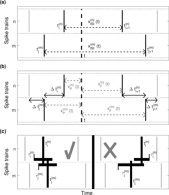
Figure 1: Schematic drawing for all three measures. (a) Illustration of the variables used to define the A-ISI-distance. All measures use the instantaneous interspike interval $x_{ISI}^{(n)}(t)$ to adapt to the local firing rate. (b) Additional variables used for the A-SPIKE-distance. (c) Coincidence criterion for the A-SPIKE-synchronization. The coincidence window of each spike is derived from the two surrounding interspike intervals. For simplicity the $thr=0$ case is shown. Here we illustrate two different examples. The two spikes on the left side are considered coincident since both lie in each other’s coincidence windows. On the right there is no coincidence because the spike from the second spike train is outside of the coincidence window from the spike of the first spike train.

2.1 Adaptive ISI-distance

The A-ISI-distance Satuvuori17 measures the instantaneous rate difference between spike trains (see Fig. 1a). It relies on a time-resolved profile, meaning that in a first step a dissimilarity value is assigned to each time instant. To obtain this profile, we first assign to each time instant $t$ the times of the previous spike and the following spike

$$t_{\mathrm{P}}^{(n)}(t)=\max\{t_{i}^{(n)}|t_{i}^{(n)}\leq t\}\quad\textrm{for }\quad t_{1}^{(n)}\leqslant t\leqslant t_{M_{n}}^{(n)}$$ (1)

$$t_{\mathrm{F}}^{(n)}(t)=\min\{t_{i}^{(n)}|t_{i}^{(n)}>t\}\quad\textrm{for }\quad t_{1}^{(n)}\leqslant t\leqslant t_{M_{n}}^{(n)}.$$ (2)

From this for each spike train $n$ an instantaneous ISI can be calculated as

$$x_{\mathrm{ISI}}^{(n)}(t)=t_{\mathrm{F}}^{(n)}(t)-t_{\mathrm{P}}^{(n)}(t).$$ (3)

The A-ISI-profile is defined as a normalized instantaneous ratio in ISIs:

$$I_{n,m}^{A}(t)=\frac{|x_{\mathrm{ISI}}^{(n)}(t)-x_{\mathrm{ISI}}^{(m)}(t)|}{\max\{x_{\mathrm{ISI}}^{(n)}(t),x_{\mathrm{ISI}}^{(m)}(t),thr\}}.$$ (4)

For the A-ISI-distance the MRTS is defined so that when the ISI of both spike trains are smaller than a threshold value $thr$, the threshold value is used instead. The multivariate A-ISI-profile is obtained by averaging over all pairwise A-ISI-profiles:

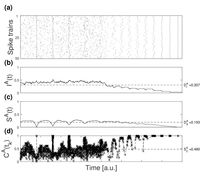
Figure 2: Profiles of A-ISI-distance (a), A-SPIKE-distance (b) and A-SPIKE-synchronization (c) for an artificial example dataset of 50 spike trains with population events with different jitters and decreasing noise over time.

$$I^{A}(t)=\frac{1}{N(N-1)/2}\sum_{n=1}^{N-1}\sum_{m=n+1}^{N}I_{n,m}^{A}(t).$$ (5)

This is a non-continuous piecewise constant profile and integrating over time gives the A-ISI-distance:

$$D_{I}^{A}=\frac{1}{t_{e}-t_{s}}\int_{t_{s}}^{t_{e}}I^{A}(t)dt.$$ (6)

Where $t_{s}$ and $t_{e}$ are the start and end times of the recording respectively. If thr is set to zero, the method falls back to the ISI-distance Kreuz07c .

Fig. 2a shows an artificial spike train dataset together with the corresponding A-ISI-profile in Fig. 2b. The A-ISI-profile for the example dataset shows high dissimilarity for the left side of the raster plot, where noise is high. When the noise is decreased and rates become more similar in the right side, the dissimilarity profile goes down. The overall ISI-distance is the mean value of the profile.

2.2 Adaptive SPIKE-distance

The A-SPIKE-distance Satuvuori17 measures the accuracy of spike times between spike trains relative to local firing rates (see Fig. 1b). In order to assess the accuracy of spike events, each spike is assigned a distance to its nearest neighbour in the other spike train:

$$\Delta t_{i}^{(n)}=\min_{j}(|t_{i}^{(n)}-t_{j}^{(m)}|).$$ (7)

The distances are interpolated between spikes using for all times $t$ the time differences to the previous and to the following spikes ${x_{P}^{(n)}(t)}$ and ${x_{F}^{(n)}(t)}$:

$$x_{P}^{(n)}(t)=t-t_{i}^{(n)}\quad\textrm{for }\quad t_{i}^{(n)}\leqslant t\leqslant t_{i+1}^{(n)}$$ (8)

$$x_{F}^{(n)}(t)=t_{i+1}^{(n)}-t\quad\textrm{for }\quad t_{i}^{(n)}\leqslant t\leqslant t_{i+1}^{(n)}.$$ (9)

These equations provide time-resolved quantities needed to define time-resolved dissimilarity profile from discrete values the same way as Eqs. 1 and 2 provide them for A-ISI-distance. The weighted spike time difference for a spike train is then calculated as an interpolation from one difference to the next by

$$S_{n}(t)=\frac{\Delta t_{i}^{(n)}(t)x_{F}^{(n)}(t)+\Delta t_{i+1}^{(n)}(t)x_{P}^{(n)}(t)}{x_{\mathrm{ISI}}^{(n)}(t)}\quad,\quad t_{i}^{(n)}\leqslant t\leqslant t_{i+1}^{(n)}.$$ (10)

This continuous function is analogous to term ${x_{\mathrm{ISI}}^{(n)}}$ for the ISI-distance, except that it is piecewise linear instead of piecewise constant. The pairwise A-SPIKE-distance profile is calculated by temporally averaging the weighted spike time differences, normalizing to the local firing rate average and, finally, weighting each profile by the instantaneous firing rates of the two spike trains:

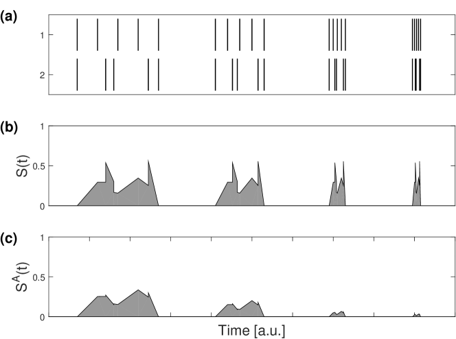
Figure 3: An example spike train pair and its SPIKE-distance and A-SPIKE-distance profiles. (a) Two spike trains having four events with five spikes per event in each spike train. The sequence of spikes in all four events is the same but the event is increasingly compressed. The only thing that changes is the time-scale. From a global perspective the first event consists of non-synchronous individual spikes, while the last event consists of coincident bursts. The two events in the middle are intermediates. (b) The SPIKE-distance $S(t)$ looks only at the local context and has the same profile shape for all events. (c) The A-SPIKE-distance considers also the global context and judges the first event like the SPIKE-distance as being dissimilar, but scales down the small spike time differences in the burst and considers the coincident burst as very similar.

$$S_{m,n}^{A}(t)=\frac{S_{n}x_{\mathrm{ISI}}^{m}(t)+S_{m}x_{\mathrm{ISI}}^{n}(t)}{2\langle x_{\mathrm{ISI}}^{n,m}(t)\rangle\max\{\langle x_{\mathrm{ISI}}^{n,m}(t)\rangle,thr\}},$$ (11)

where $\langle x_{\mathrm{ISI}}^{n,m}(t)\rangle$ is the mean over the two instantaneous ISIs. MRTS is defined by using a threshold, that replaces the denominator of weighting to spike time differences if the mean is smaller than the $thr$. This profile is analogous to the pairwise A-ISI-profile ${I_{n,m}^{A}(t)}$, but again it is piecewise linear, not piecewise constant. Unlike $S_{n}(t)$ it is not continuous, typically it exhibits instantaneous jumps at the times of the spikes. The multivariate A-SPIKE-profile is obtained the same way as the multivariate A-ISI-profile, by averaging over all pairwise profiles:

$$S^{A}(t)=\frac{1}{N(N-1)/2}\sum_{n=1}^{N-1}\sum_{m=n+1}^{N}S_{m,n}^{A}(t).$$ (12)

The final A-SPIKE-distance is calculated as the time integral over the multivariate A-SPIKE-profile the same way as the A-ISI-distance:

$$D_{S}^{A}=\frac{1}{t_{e}-t_{s}}\int_{t_{s}}^{t_{e}}S^{A}(t)dt.$$ (13)

The effect of applying the threshold can be seen in Fig. 3. With $thr=0$ the method falls back to the regular SPIKE-distance Kreuz11 . The A-SPIKE-profile for the artificial test dataset in Fig. 2c goes to zero when the spikes in all spike trains appear at the exactly same time.

2.3 Adaptive SPIKE-synchronization

A-SPIKE-synchronization Satuvuori17 quantifies how many of the possible coincidences in a dataset are actually coincidences (Fig. 1c). While the A-ISI-distance and the A-SPIKE-distance are measures of dissimilarity which obtain low values for similar spike trains, A-SPIKE-synchronization measures similarity. If all the spikes are coincident with a spike in all the other spike trains, the value will be one. In contrast, if none of the spikes are coincident, it will be zero.

The original SPIKE-synchronization Kreuz15 is parameter- and time-scale-free, since it uses the adaptive coincidence detection which was first proposed for the measure Event synchronization QuianQuiroga02b . The coincidence window, i.e., the time lag below which two spikes from two different spike trains, $t_{i}^{(n)}$ and $t_{j}^{(m)}$, are considered to be coincident, is adapted to the local firing rate. Spikes are coincident only if they both lie in each others coincidence windows. A-SPIKE-synchronization is a generalized version of the SPIKE-synchronization. The MRTS is used to decide if the window is determined locally or if the global context should be taken into account.

As a first step, we define the ISI before and after the spike as

$$x_{iP}^{(n)}=\lim_{t\to t_{i}-}x_{\mathrm{ISI}}^{(n)}(t)$$ (14)

$$x_{iF}^{(n)}=\lim_{t\to t_{i}+}x_{\mathrm{ISI}}^{(n)}(t).$$ (15)

The coincidence window for spike $i$ of spike train $n$ is defined by determining a minimum coincidence window size for a spike as half of the ISIs adjacent to the spike and allowing asymmetric coincidence windows based on MRTS. This is done by using $thr$ instead of the minimum, if it is smaller. Since the threshold value is based on ISIs and the coincidence window spans both sides of the spike, only half of the threshold spans each side. For the A-ISI- and the A-SPIKE-distance the changes induced by the threshold appear gradually, but for A-SPIKE-synchronization it is a sudden change from a non-coincidence to coincidence for a spike. Therefore, due to the binary nature of A-SPIKE-synchronization, the threshold is additionally divided by two. The coincidence window is not allowed to overlap with a coincidence window of another spike and is thus limited to half the ISI even if the threshold is larger. The base of the window is defined by the two adjacent ISIs:

$$\tau_{i}^{(n)}=\frac{1}{2}\min\{x_{iP}^{(n)},x_{iF}^{(n)}\}.$$ (16)

The coincidence window of a spike is then defined in an asymmetric form by using the coincidence window part before and after the spike as

$$\tau_{iP}^{(n)}=\min\{\max(\frac{1}{4}thr,\tau_{i}^{(n)}),\frac{1}{2}x_{iP}^{(n)}\}$$ (17)

$$\tau_{iF}^{(n)}=\min\{\max(\frac{1}{4}thr,\tau_{i}^{(n)}),\frac{1}{2}x_{iF}^{(n)}\}.$$ (18)

The combined coincidence window for spikes $i$ and $j$ is then defined as

$$\tau_{ij}^{(n,m)}=\begin{cases}\min\{\tau_{iF}^{(n)},\tau_{jP}^{(m)}\}&{\rm if}~{}~{}t_{i}\leqslant t_{j}\cr\min\{\tau_{iP}^{(n)},\tau_{jF}^{(m)}\}&otherwise\end{cases}.$$ (19)

The coincidence criterion can be quantified by means of a coincidence indicator

$$C_{i}^{(n,m)}=\begin{cases}1&{\rm if}~{}~{}\min_{j}\{|t_{i}^{(n)}-t_{j}^{(m)}|\}<\tau_{ij}^{(n,m)}\cr 0&{\rm otherwise}\end{cases}.$$ (20)

This definition ensures that each spike can only be coincident with at most one spike in the other spike train. The coincidence criterion assigns either a one or a zero to each spike depending on whether it is part of a coincidence or not. For each spike of every spike train, a normalized coincidence counter

$$C_{i}^{(n)}=\frac{1}{N-1}\sum_{m\neq n}C_{i}^{(n,m)}$$ (21)

is obtained by averaging over all $N-1$ bivariate coincidence indicators involving the spike $i$ in spike train $n$.

This way we have defined a coincidence indicator for each individual spike in the spike trains. In order to obtain one combined similarity profile, we pool the spikes of the spike trains as well as their coincidence indicators by introducing one overall spike index $k$ and defining

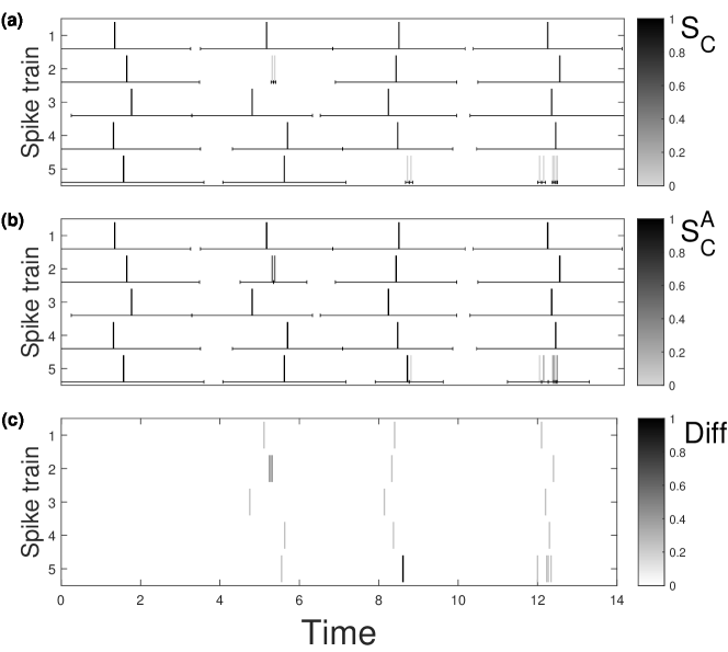
Figure 4: SPIKE-synchronization, A-SPIKE-synchronization and their difference illustrated using five spike trains with four simple events. Without the correction (A) in case of spike doublets (first and second event) or bursts (third event) the small interspike intervals result in an unreasonably high demand for spike timing accuracy. With the adaptive correction (B) for all these cases the likelihood increases that at least one of the spikes is part of a coincidence. On the other hand, if there are no doublets or bursts (last event), nothing changes (best seen in C). Note that for better visibility the colour scales differ, we use grey-black in A and B and white-black in C.

$$M=\sum_{n=1}^{N}M_{n}.$$ (22)

This yields one unified set of coincidence indicators $C_{k}$:

$$\{C_{k}\}=\bigcup_{n}\{C_{i}^{(n)}\}.$$ (23)

From this discrete set of coincidence indicators $C_{k}$ the A-SPIKE-synchronization profile $C^{A}(t_{k})$ is obtained by $C^{A}(t_{k})=C_{k}$.

Finally, A-SPIKE-synchronization is defined as the average value of this profile

$$S_{C}^{A}=\frac{1}{M}\sum_{k=1}^{M}C^{A}(t_{k}).$$ (24)

It is important to note that since A-SPIKE-synchronization is a measure of similarity, reducing differences below threshold adds coincidences and thus the value obtained increases. In Fig. 4 we illustrate how the asymmetric coincidence windows of A-SPIKE-synchronization allow for a better coverage of burst events which makes it easier to match spikes when compared to SPIKE-synchronization ($thr=0$) Kreuz15 .

As can be seen in Fig. 2d, the A-SPIKE-synchronization profile is discrete and only defined at spike times. A dotted line between the points is added as visual aid. The profile gets higher values the more coincidences are found for each spike in other spike trains.

2.4 Selecting the threshold value

In some cases spikes that occur less than a second apart might be considered more simultaneous than those taking place within minutes, and in applications like meteorological systems, weeks instead of months. Setting the minimum relevant time-scale might not be a simple task. If no information of the system producing the spikes is available, all one can do to estimate an appropriate threshold value is to look at the ISIs.

There are two criteria that a threshold value extracted from the data has to fulfil. First of all it needs to adapt to changes in spike count so that adding more spikes gives shorter threshold. Additionally we want the threshold to adapt to changes in the ISI-distribution when the spike count is fixed. The more pronounced bursts are found in the data, the more likely any differences within aligned bursts are not as important as their placement. Thus, we want our threshold to get longer if the spikes are packed together. To do so, all the ISIs in all spike trains are pooled and the threshold is determined from the pooled ISI distribution.

One should not just take a value based on ISI-distribution that counts the interspike intervals, as the mean does, but weight them by their length, which is equivalent to taking the average of the second moments of ISIs. Doing this reduces the importance of very short ISIs even if they are statistically much more common. In order to obtain a value with the right dimension, the square root of the average must be taken:

$$thr=\sqrt{\langle{(L_{\mathrm{ISI}})^{2}}\rangle}=\sqrt{\frac{\sum_{n=1}^{N}a_{n}{L_{\mathrm{ISI}}^{n}}^{2}}{\sum_{n=1}^{N}a_{n}}}.$$ (25)

Here we denoted a single ISI length in the pooled distribution as $L_{\mathrm{ISI}}^{n}$ and the number of ISI with length $L_{\mathrm{ISI}}^{n}$ as $a_{n}$. It is important to note, however, that this is only an estimate based on different time-scales found in the data. The selected MRTS is not an indicator of a time-scale of the system that produced the spikes.

As an example of how the threshold works we apply the threshold to Gamma $\Gamma(k,x)$ distribution. Since the kurtosis of the distribution is proportional to $1/k$, for small k the distribution contains large number of small ISI and few long ones.This is the property the threshold is tracking. The mean of a gamma distribution is $k/x$ and the second moment $(k+1)k/x$. thus the ratio of the threshold and the mean ISI is $thr/\langle{L_{\mathrm{ISI}}}\rangle=\sqrt{x(k+1)/k}$. From the formula we can see that for small k, where the distribution is more skewed, the ratio between the mean ISI and the threshold increases. This means that mainly the rare and large inter-burst ISIs are taken into account.

The threshold value determines the outcome of the adaptive methods. However, the threshold is not a hard set limiter neglecting everything below the threshold, but rather the point from which on differences are considered in a global instead of a local context.

3 Measures of spike train directionality

Often a set of spike trains exhibits well-defined patterns of spatio-temporal propagation where some prominent feature first appears at a specific location and then spreads to other areas until potentially becoming a global event. If a set of spike trains exhibits perfectly consistent repetitions of the same global propagation pattern, this can be called a synfire pattern. For any spike train set exhibiting propagation patterns the questions arises naturally whether these patterns show any consistency, i.e., to what extent do the spike trains resemble a synfire pattern, are there spike trains that consistently lead global events and are there other spike trains that invariably follow these leaders?

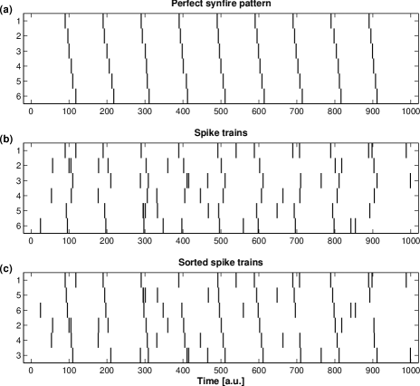
Figure 5: Motivation for SPIKE-order and Spike Train Order. (a) Perfect Synfire pattern. (b) Unsorted set of spike trains. (c) The same spike trains as in (b) but now sorted from leader to follower.

In the second part of this chapter we describe a framework consisting of two directional measures (SPIKE-Order and Spike Train Order) that allows to define a value termed Synfire Indicator which quantifies the consistency of the leader-follower relationships Kreuz2016 . This Synfire Indicator attains its maximal value of $1$ for a perfect synfire pattern in which all neurons fire repeatedly in a consistent order from leader to follower (Fig. 5a).

The same framework also allows to sort multiple spike trains from leader to follower, as illustrated in Figs. 5b and 5c. This is meant purely in the sense of temporal sequence. Whereas Fig. 5b shows an artificially created but rather realistic spike train set, in Fig. 5c the same spike trains have been sorted to become as close as possible to a synfire pattern. Now the spike trains that tend to fire first are on top whereas spike trains with predominantly trailing spikes are at the bottom.

Analyzing leader-follower relationships in a spike train set requires a criterion that determines which spikes should be compared against each other. What is needed is a match maker, a method which pairs spikes in such a way that each spike is matched with at most one spike in each of the other spike trains. This match maker already exists. It is the adaptive coincidence detection first used as the fundamental ingredient for the bivariate measure SPIKE-synchronization Kreuz15 (see Section 2.3).

3.1 SPIKE-Order and Spike Train Order

The symmetric measure SPIKE-Synchronization (introduced in Section 2.3) assigns to each spike of a given spike train pair a bivariate coincidence indicator. These coincidence indicators $C_{i}^{(n,m)}$ (Eq. 20), which are either $0$ or $1$, are then averaged over spike train pairs and converted into one overall profile $C(t_{k})$ normalized between $0$ and $1$. In exactly the same manner SPIKE-Order and Spike Train Order assign bivariate order indicators to spikes. Also these two order indicators, the asymmetric $D_{i}^{(n,m)}$ and the symmetric $E_{i}^{(n,m)}$, which both can take the values $-1$, $0$, or $+1$, are averaged over spike train pairs and converted into two overall profiles $D(t_{k})$ and $E(t_{k})$ which are normalized between $-1$ and $1$. The SPIKE-Order profile $D(t_{k})$ distinguishes leading and following spikes, whereas the Spike Train Order profile $E(t_{k})$ provides information about the order of spike trains, i.e. it allows to sort spike trains from leaders to followers.

First of all, the symmetric coincidence indicator $C^{(n,m)}_{i}$ of SPIKE-Synchronization (Eq. 20) is replaced by the asymmetric SPIKE-Order indicator

$$D_{i}^{(n,m)}=C_{i}^{(n,m)}\cdot\operatorname{\operatorname{sign}}(t_{j}^{(m)}-t_{i}^{(n)}),$$ (26)

where the index $j$ is defined from the minimum in Eq. 20 with the threshold-value in Eqs. 17 and 18 set to $thr=0$.

The corresponding value $D_{j}^{(m,n)}$ is obtained in an asymmetric manner as

$$D_{j}^{(m,n)}=C_{j}^{(m,n)}\cdot\operatorname{\operatorname{sign}}(t_{i}^{(n)}-t_{j}^{(m)})=-D_{i}^{(n,m)}.$$ (27)

Therefore, this indicator assigns to each spike either a $1$ or a $-1$ depending on whether the respective spike is leading or following a coincident spike from the other spike train. The value $0$ is obtained for cases in which there is no coincident spike in the other spike train ($C^{(n,m)}_{i}=0$), but also in cases in which the times of the two coincident spikes are absolutely identical ($t_{j}^{(m)}=t_{i}^{(n)}$).

The multivariate profile $D(t_{k})$ obtained analogously to Eq. 23 is normalized between $1$ and $-1$ and the extreme values are obtained if a spike is either leading ($+1$) or following ($-1$) coincident spikes in all other spike trains. It can be $0$ either if a spike is not part of any coincidences or if it leads exactly as many spikes from other spike trains in coincidences as it follows. From the definition in Eqs. 26 and 27 it follows immediately that $C_{k}$ is an upper bound for the absolute value $|D_{k}|$.

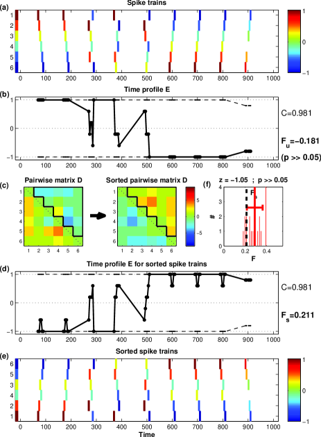
Figure 6: Illustration of SPIKE-Order for an artificially created example dataset consisting of $6$ spike trains which emit spikes in nine reliable events. For the first two events spikes fire in order, for the next three events the order is random whereas for the last four events the order is inverted. In the last event there is one spike missing. (a) Unsorted spike trains with the spikes color-coded according to the value of the SPIKE-Order $D(t_{k})$. (b) Spike Train Order profile $E(t_{k})$. Events with different firing order can clearly be distinguished. The SPIKE-Synchronization profile $C(t_{k})$ and its mirror profile (dashed black lines) act as envelope. The Synfire Indicator $F_{u}$ for the unsorted spike trains is slightly negative reflecting the dominance of the inversely ordered events. (c) Pairwise cumulative SPIKE-Order matrix $D$ before (left) and after (right) sorting. The optimal order maximizes the upper triangular matrix $D_{(n<m)}$, marked in black. The thick black arrow in between the two matrices indicates the sorting process. (d) Spike Train Order profile $E(t_{k})$ and its average values, the Synfire Indicator $F_{s}$ for the sorted spike trains. (e) Sorted spike trains. (f) Statistical significance: Results of the surrogate analysis. Thick lines denote mean and standard deviation for $19$ surrogates. Since the value for the original dataset (black) is not maximum, the optimally sorted spike trains do not exhibit a statistically significant synfire pattern.

In Fig. 6 we show the application of the SPIKE-Order framework to an example dataset. While the SPIKE-Order profile can be very useful for color-coding and visualizing local spike leaders and followers (Fig. 6a), it is not useful as an overall indicator of Spike Train Order. The profile is invariant under exchange of spike trains, i.e. it looks the same for all events no matter what the order of the firing is (in our example only the last event looks slightly different since one spike is missing). Moreover, summing over all profile values, which is equivalent to summing over all coincidences, necessarily leads to an average value of $0$, since for every leading spike ($+1$) there has to be a following spike ($-1$).

So in order to quantify any kind of leader-follower information between spike trains we need a second kind of order indicator. The Spike Train Order indicator is similar to the SPIKE-Order indicator defined in Eqs. 26 and 27 but with two important differences. Both spikes are assigned the same value and this value now depends on the order of the spike trains:

$$E_{i}^{(n,m)}=C_{i}^{(n,m)}\cdot\begin{cases}\operatorname{\operatorname{sign}}(t_{j}^{(m)}-t_{i}^{(n)})\quad\text{if}\quad n<m\\ \operatorname{\operatorname{sign}}(t_{i}^{(n)}-t_{j}^{(m)})\quad\text{if}\quad n>m\end{cases}$$ (28)

and

$$E_{j}^{(m,n)}=E_{i}^{(n,m)}.$$ (29)

This symmetric indicator assigns to both spikes a $+1$ in case the two spikes are in the correct order, i.e. the spike from the spike train with the lower spike train index is leading the coincidence, and a $-1$ in the opposite case. Once more the value $0$ is obtained when there is no coincident spike in the other spike train or when the two coincident spikes are absolutely identical.

The multivariate profile $E(t_{k})$, again obtained similarly to Eq. 23, is also normalized between $1$ and $-1$ and the extreme values are obtained for a coincident event covering all spike trains with all spikes emitted in the order from first (last) to last (first) spike train, respectively (see the first two and the last four events in Fig. 6). It can be $0$ either if a spike is not a part of any coincidences or if the order is such that correctly and incorrectly ordered spike train pairs cancel each other. Again, $C_{k}$ is an upper bound for the absolute value of $E_{k}$.

3.2 Synfire Indicator

In contrast to the SPIKE-Order profile $D_{k}$, for the Spike Train Order profile $E_{k}$ it does make sense to define an average value, which we term the Synfire Indicator:

$$F=\frac{1}{M}\sum_{k=1}^{M}E(t_{k}).$$ (30)

The interpretation is very intuitive. The Synfire Indicator $F$ quantifies to what degree the spike trains in their current order resemble a perfect synfire pattern. It is normalized between $1$ and $-1$ and attains the value $1$ ($-1$) if the spike trains in their current order form a perfect (inverse) synfire pattern, meaning that all spikes are coincident with spikes in all other spike trains and that the order from leading (following) to following (leading) spike train remains consistent for all of these events. It is $0$ either if the spike trains do not contain any coincidences at all or if among all spike trains there is a complete symmetry between leading and following spikes.

The Spike Train Order profile $E(t_{k})$ for our example is shown in Fig. 6c. In this case the order of spikes within an event clearly matters. The Synfire Indicator $F$ is slightly negative indicating that the current order of the spike trains is actually closer to an inverse synfire pattern.

Given a set of spike trains we now would like to sort the spike trains from leader to follower such that the set comes as close as possible to a synfire pattern. To do so we have to maximize the overall number of correctly ordered coincidences and this is equivalent to maximizing the Synfire Indicator $F$. However, it would be very difficult to achieve this maximization by means of the multivariate profile $E(t_{k})$. Clearly, it is more efficient to sort the spike trains based on a pairwise analysis of the spike trains. The most intuitive way is to use the anti-symmetric cumulative SPIKE-Order matrix

$$D^{(n,m)}=\sum_{i}D_{i}^{(n,m)}$$ (31)

which sums up orders of coincidences from the respective pair of spike trains only and quantifies how much spike train $n$ is leading spike train $m$ (Fig. 6c).

Hence if $D^{(n,m)}>0$ spike train $n$ is leading $m$, while $D^{(n,m)}<0$ means $m$ is leading $n$. If the current Spike Train Order is consistent with the synfire property, we thus expect that $D^{(n,m)}>0$ for $n<m$ and $D^{(n,m)}<0$ for $n>m$. Therefore, we construct the overall SPIKE-Order as

$$D_{(n<m)}=\sum_{n<m}D^{(n,m)},$$ (32)

i.e. the sum over the upper right tridiagonal part of the matrix $D^{(n,m)}$.

After normalizing by the overall number of possible coincidences, we arrive at a second more practical definition of the Synfire Indicator:

$$F=\frac{2D_{(n<m)}}{(N-1)M}.$$ (33)

The value is identical to the one of Eq. 30, only the temporal and the spatial summation of coincidences (i.e., over the profile and over spike train pairs) are performed in the opposite order.

Having such a quantification depending on the order of spike trains, we can introduce a new ordering in terms of the spike train index permutation $\varphi(n)$. The overall Synfire Indicator for this permutation is then denoted as $F_{\varphi}$. Accordingly, for the initial (unsorted) order of spike trains $\varphi_{u}$ the Synfire Indicator is denoted as $F_{u}=F_{\varphi_{u}}$.

The aim of the analysis is now to find the optimal (sorted) order $\varphi_{s}$ as the one resulting in the maximal overall Synfire Indicator $F_{s}=F_{\varphi_{s}}$:

$$\varphi_{s}:F_{\varphi_{s}}=\max_{\varphi}\{F_{\varphi}\}=F_{s}.$$ (34)

This Synfire Indicator for the sorted spike trains quantifies how close spike trains can be sorted to resemble a synfire pattern, i.e., to what extent coinciding spike pairs with correct order prevail over coinciding spike pairs with incorrect order. Unlike the Synfire Indicator for the unsorted spike trains $F_{u}$, the optimized Synfire Indicator $F_{s}$ can only attain values between $0$ and $1$ (any order that yields a negative result could simply be reversed in order to obtain the same positive value). For a perfect synfire pattern we obtain $F_{s}=1$, while sufficiently long Poisson spike trains without any synfire structure yield $F_{s}\approx 0$.

The complexity of the problem to find the optimal Spike Train Order is similar to the well-known travelling salesman problem Applegate11 . For $N$ spike trains there are $N!$ permutations $\varphi$, so for large numbers of spike trains finding the optimal Spike Train Order $\varphi_{s}$ is a non-trivial problem and brute-force methods such as calculating the $F_{\varphi}$-value for all possible permutations are not feasible. Instead, we search for the optimal order using simulated annealing Dowsland12 , a probabilistic technique which approximates the global optimum of a given function in a large search space. In our case this function is the Synfire Indicator $F_{\varphi}$ (which we would like to maximize) and the search space is the permutation space of all spike trains. We start with the $F_{u}$-value from the unsorted permutation and then visit nearby permutations using the fundamental move of exchanging two neighboring spike trains within the current permutation. All moves with positive $\Delta F$ are accepted while the likelihood of accepting moves with negative $\Delta F$ is decreased along the way according to a standard slow cooling scheme. The procedure is repeated iteratively until the order of the spike trains no longer changes or until a predefined end temperature is reached.

The sorting of the spike trains maximizes the Synfire Indicator as reflected by both the normalized sum of the upper right half of the pairwise cumulative SPIKE-Order matrix (Eq.33, Fig. 6c) and the average value of the Spike Train Order profile $E(t_{k})$ (Eq.30, Fig. 6d). Finally, the sorted spike trains in Fig. 6e are now ordered such that the first spike trains have predominantly high values (red) and the last spike trains predominantly low values (blue) of $D(t_{k})$.

The complete analysis returns results consisting of several levels of information. Time-resolved (local) information is represented in the spike-coloring and in the profiles $D$ and $E$. The pairwise information in the SPIKE-order matrix reflects the leader-follower relationship between two spike trains at a time. The Synfire Indicator $F$ characterizes the closeness of the dataset as a whole to a synfire pattern, both for the unsorted ($F_{u}$) and for the sorted ($F_{s}$) spike trains. Finally, the sorted order of the spike trains is a very important result in itself since it identifies the leading and the following spike trains.

3.3 Statistical significance

As a last step in the analysis we evaluate the statistical significance of the optimized Synfire Indicator $F_{s}$ using a set of carefully constructed spike train surrogates. The idea behind the surrogate test is to estimate the likelihood that the consistent SPIKE-Order pattern yielding a certain Synfire Indicator could have been obtained by chance. To this aim, for each surrogate we maintain the coincidence structure of the spike trains by keeping the SPIKE-Synchronization values of each individual spike constant but randomly swap the spike order in a sufficient number of coincidences. We set the number of swaps equal to the number of coincident spikes in the dataset since this way all possible spike order patterns can be reached. Only for the first surrogate we swap twice as many coincidences in order to account for transients. After each swap we take extra care that all other spike orders that are affected by the swap are updated as well. For example, if a swap changes the order between the first and the third spike in an ordered sequence of three spikes, we also swap both the order between the first and the second and the order between the second and the third spike.

For each spike train surrogate we repeat exactly the same optimization procedure in the spike train permutation space that is done for the original dataset. The original Synfire Indicator is deemed significant if it is higher than the Synfire Indicator obtained for all of the surrogate datasets (this case will be marked by two asterisks). Here we use $s=19$ surrogates for a significance level of $p^{*}=1/(s+1)=0.05$. Note that in order to achieve a better sampling of the underlying null distribution a larger number of surrogates would be preferable but the chosen value of $s$ is a compromise that takes into account the computational cost. As a second indicator we state the z-score, e.g., the deviation of the original value $x$ from the mean $\mu$ of the surrogates in units of their standard deviation $\sigma$:

$$z=\frac{x-\mu}{\sigma}.$$ (35)

Results of the significance analysis for our standard example are shown in the histogram in Fig. 6f. In this case the absolute value of the z-score is smaller than one and the p-value is larger than $p^{*}$ and the result is thus judged as statistically non-significant.

4 Outlook

In the first part of this chapter we describe three parameter-free and time resolved measures of spike train synchrony in their recently developed adaptive extensions, A-ISI-distance, A-SPIKE-distance and A-SPIKE-synchronization Satuvuori17 . All of these measures are symmetric and so their multivariate versions are invariant to changes in the order of spike trains. Since information about directionality is very relevant, in the second part of this chapter we show an algorithm which allows to sort multiple spike trains from leader to follower. This algorithm is built on two indicators, SPIKE-Order and Spike Train Order, that define the Synfire Indicator value, which quantifies the consistency of the temporal leader-follower relationships for both the original and the optimized sorting.

Symmetric measures of spike train distances (Section 2) have been applied in many different contexts, not only in the field of neuroscience Jolivet08 ; Mainen95 ; Victor05 . For example, they have been used in robotics Espinal16 and prosthesis control Dura-Bernal16 . The ISI-distance has been applied in a method for the detection of directionl coupling between point processes and point processes and flows Andrzejak11 , as an adaptation of the nonlinear technique for directional coupling detection of continuous signals Chicharro09b .

Questions about leader-follower dynamics (Section 3) have been specifically investigated in neuroscience Pereda05 , but also in fields as wide-ranging as, e.g., climatology Boers14 , social communication Varni10 , and human-robot interaction Rahbar15 . SPIKE-Order has already been applied to analyze the consistency of propagation patterns in two real datasets from neuroscience (Giant Depolarized Potentials in mice slices) and climatology (El Niño sea surface temperature recordings) Kreuz2016 .

Finally, we would like to mention that the similarity measures A-ISI-distance, A-SPIKE-distance and A-SPIKE-synchronization, as well as SPIKE-Order, are implemented in three publicly available software packages, the Matlab-based graphical user interface SPIKY Kreuz15 , cSPIKE (Matlab command line with MEX-files), and the open-source Python library PySpike Mulansky16 .

- [1] R. G. Andrzejak and T. Kreuz. Characterizing unidirectional couplings between point processes and flows. Europhysics Letters, 96:50012, 2011.
- [2] D. L. Applegate, R. E. Bixby, V. Chvatal, and W. J. Cook. The traveling salesman problem: a computational study. Princeton University Press, 2011.
- [3] N. Boers, B. Bookhagen, H.M.J. Barbosa, N. Marwan, J. Kurths, and J.A. Marengo. Prediction of extreme floods in the eastern central andes based on a complex networks approach. Nature Communications, 5:5199, 2014.
- [4] M. R. Bower, M. Stead, F. B. Meyer, W. R. Marsh, and G. A. Worrell. Spatiotemporal neuronal correlates of seizure generation in focal epilepsy. Epilepsia, 53:807, 2012.
- [5] D. Chicharro and R. G. Andrzejak. Reliable detection of directional couplings using rank statistics. Physical Review E, 80(2):026217, 2009.
- [6] D. Chicharro, T. Kreuz, and R. G. Andrzejak. What can spike train distances tell us about the neural code? J Neurosci Methods, 199:146–165, 2011.
- [7] K. A. Dowsland and J. M. Thompson. Simulated annealing. In Handbook of Natural Computing, pages 1623–1655. Springer, 2012.
- [8] S. Dura-Bernal, K. Li, S. A. Neymotin, J. T. Francis, J. C. Principe, and W. W. Lytton. Restoring behavior via inverse neurocontroller in a lesioned cortical spiking model driving a virtual arm. Frontiers in Neuroscience, 10, 2016.
- [9] A. Espinal, H. Rostro-Gonzalez, M. Carpio, E. I. Guerra-Hernandez, M. Ornelas-Rodriguez, H. J. Puga-Soberanes, M. A. Sotelo-Figuero, and P. Melin. Quadrupedal robot locomotion: a biologically inspired approach and its hardware implementation. Computational Intelligence and Neuroscience, page 5615618, 2016.
- [10] R. Jolivet, R. Kobayashi, A. Rauch, R. Naud, S. Shinomoto, and W. Gerstner. A benchmark test for a quantitative assessment of simple neuron models. J Neurosci Methods, 169:417, 2008.
- [11] T. Kreuz. Synchronization measures. In R. Quian Quiroga and S. Panzeri, editors, Principles of neural coding, page p. 97. CRC Taylor and Francis, Boca Raton, FL, USA, 2013.
- [12] T. Kreuz, D. Chicharro, M. Greschner, and R. G. Andrzejak. Time-resolved and time-scale adaptive measures of spike train synchrony. J Neurosci Methods, 195:92, 2011.
- [13] T. Kreuz, D. Chicharro, C. Houghton, R. G. Andrzejak, and F. Mormann. Monitoring spike train synchrony. J Neurophysiology, 109:1457, 2013.
- [14] T. Kreuz, J. S. Haas, A. Morelli, H. D. I. Abarbanel, and A. Politi. Measuring spike train synchrony. J Neurosci Methods, 165:151, 2007.
- [15] T. Kreuz, F. Mormann, R. G. Andrzejak, A. Kraskov, K. Lehnertz, and P. Grassberger. Measuring synchronization in coupled model systems: A comparison of different approaches. Phys D, 225:29, 2007.
- [16] T. Kreuz, M. Mulansky, and N. Bozanic. SPIKY: A graphical user interface for monitoring spike train synchrony. J Neurophysiol, 113:3432, 2015.
- [17] Thomas Kreuz, Eero Satuvuori, Martin Pofahl, and Mario Mulansky. Leaders and followers: Quantifying consistency in spatio-temporal propagation patterns. New Journal of Physics, 19:043028, 2017.
- [18] Z. Mainen and T. J. Sejnowski. Reliability of spike timing in neocortical neurons. Science, 268:1503, 1995.
- [19] M. Mulansky and T. Kreuz. Pyspike - A python library for analyzing spike train synchrony. Software X, 5:183–189, 2016.
- [20] E. Pereda, R. Quian Quiroga, and J. Bhattacharya. Nonlinear multivariate analysis of neurophysiological signals. Progress in Neurobiology, 77:1, 2005.
- [21] R. Quian Quiroga, T. Kreuz, and P. Grassberger. Event synchronization: A simple and fast method to measure synchronicity and time delay patterns. Phys. Rev. E, 66:041904, 2002.
- [22] F. Rahbar, S. Anzalone, G. Varni, E. Zibetti, S. Ivaldi, and M. Chetouani. Predicting extraversion from non-verbal features during a face-to-face human-robot interaction. International Conference on Social Robotics, page 10, 2015.
- [23] E. Satuvuori, M. Mulansky, N. Bozanic, K. Lenk, and T. Kreuz. Generalizing definitions of ISI-distance, SPIKE-distance and SPIKE-synchronization. In preparation, 2017.
- [24] W. Truccolo, J. A. Donoghue, L. R. Hochberg, E. N. Eskandar, J. R. Madsen, W. S. Anderson, E. N. Brown, E. Halgren, and S. S. Cash. Single-neuron dynamics in human focal epilepsy. Nature Neurosci, 14:635, 2011.
- [25] M. C. W. van Rossum. A novel spike distance. Neural Computation, 13:751, 2001.
- [26] G. Varni, G. Volpe, and A. Camurri. A system for real-time multimodal analysis of nonverbal affective social interaction in user-centric media. IEEE Transactions on multimedia, 12:576, 2010.
- [27] J. D. Victor. Spike train metrics. Current Opinion in Neurobiology, 15:585, 2005.
- [28] J. D. Victor and K. P. Purpura. Nature and precision of temporal coding in visual cortex: A metric-space analysis. J Neurophysiol, 76:1310, 1996.