A unique discrimination between new physics scenarios in $b\rightarrow s\mu^{+}\mu^{-}$ anomalies

Abstract

A number of observables related to the $b\to s\ell^{+}\ell^{-}$ transition show deviations from their standard model predictions. A global fit to the current $b\rightarrow s\ell^{+}\ell^{-}$ data suggests several new physics solutions. Considering only one operator at a time and new physics only in the muon sector, it has been shown that the new physics scenarios (I) $C_{9}^{\rm NP}<0$, (II) $C_{9}^{\rm NP}=-C_{10}^{\rm NP}$, (III) $C_{9}^{\rm NP}=-C_{9}^{\prime\rm NP}$ can account for all data. In this work, we develop a procedure to uniquely identify the correct new physics solution. The scenario II predicts a significantly lower value of $\mathcal{B}(B_{s}\to\mu^{+}\mu^{-})$ and can be distinguished from the other two scenarios if the experimental uncertainty comes down by a factor of three. On the other hand, a precise measurement of the CP averaged angular observables $S_{9}$ in high $q^{2}$ bin of $B\to K^{*}\mu^{+}\mu^{-}$ decay can uniquely discriminate between the other two scenarios. We propose new methods, in terms of azimuthal angle asymmetries, to measure $S_{9}$ with the necessary precision.

I Introduction

The quark level transition $b\to s\ell^{+}\ell^{-}$ ($\ell=e,\,\mu$) has immense potential to probe physics beyond Standard Model (SM). This decay is forbidden at the tree level within the SM and hence is highly suppressed. Further, the same quark level transition induces several decay modes such as $B\to X_{s}\ell^{+}\ell^{-}$, $B\to(K,\,K^{*})\ell^{+}\ell^{-}$, $B_{s}\to\phi\ell^{+}\ell^{-}$, $B_{s}\to\ell^{+}\ell^{-}$, thus providing a plethora of observables to probe new physics (NP). Due of these reasons, the $b\to s\ell^{+}\ell^{-}$ sector plays a pivotal role in hunting physics beyond SM.

The importance of this sector has increased considerably over last few years due to the fact that several deviations from the SM have been observed in decay modes induced by $b\to s\ell^{+}\ell^{-}$. These include measurements of the lepton flavor universality (LFU) violating ratios $R_{K}$ and $R_{K^{*}}$ rkstar ; Rk2019 ; Abdesselam:2019wac ; LHCb:2021trn . The measured values of these observables disagree with their SM predictions of $\approx$ 1 Hiller:2003js ; Bordone:2016gaq at the level of $\sim 2.5-3\sigma$. This tension with the SM can be accounted by assuming new physics in $b\rightarrow s\,e^{+}\,e^{-}$ and/or $b\rightarrow s\mu^{+}\mu^{-}$ . Further, there are a few anomalous measurements which can be elucidated by considering new physics only in $b\to s\mu^{+}\mu^{-}$ transition. These include measurements of branching ratio of $B_{s}\to\phi\mu^{+}\mu^{-}$ bsphilhc2 and angular observable $P^{\prime}_{5}$ in $B\to K^{*}\mu^{+}\mu^{-}$ decay Kstarlhcb1 ; Kstarlhcb2 ; Aaij:2020nrf . The measured values disagree with the SM expectations at the $\sim 4\sigma$ level sm-angular . Hence one can account for all of these measurements simply by assuming new physics only in the muon sector.

This pile-up of anomalies in a coherent fashion can be considered as a signature of new physics (NP). This NP can be quantified in a model independent way, within the framework of effective field theory, by the addition of new operators to the SM effective Hamiltonian. Model independent analysis serves as a guideline for constructing specific new physics models which can account for these anomalies. In order to identify the Lorentz structure of possible new physics, several groups have performed global fits to all available data in the $b\to s\mu^{+}\mu^{-}$ sector Alguero:2019ptt ; Alok:2019ufo ; Ciuchini:2019usw ; DAmico:2017mtc ; Datta:2019zca ; Aebischer:2019mlg ; Kowalska:2019ley ; Arbey:2019duh ; Geng:2021nhg ; Altmannshofer:2021qrr ; Hurth:2021nsi ; Carvunis:2021jga . Most of these analyses suggested new physics solutions in the form of vector and axial-vector operators. However there is no unique solution. In the simplest approach, where only one new physics Wilson coefficient or two related new physics Wilson coefficients are considered, the following scenarios provide a good fit to all $b\to s\,\mu^{+}\,\mu^{-}$ data:

• Scenario I: In this scenario, the new physics is in the form of the operator $O_{9}=(\bar{s}\gamma^{\mu}P_{L}b)\,(\bar{\mu}\gamma^{\mu}\mu)$ alone. Its Wilson coefficient is $C_{9}=C_{9}^{\rm SM}+C_{9}^{\rm NP}$ and the data require a large negative value of the NP Wilson coefficient $C_{9}^{\rm NP}$.

• Scenario II: The NP operators of this scenario are a linear combination of $O_{9}$ and $O_{10}=(\bar{s}\gamma^{\mu}P_{L}b)\,(\bar{\mu}\gamma^{\mu}\gamma^{5}\mu)$. The Wilson coefficient of the latter operator is $C_{10}=C_{10}^{\rm SM}+C_{10}^{\rm NP}$. The data imposes the condition $C_{9}^{\rm NP}=-C_{10}^{\rm NP}$ on the NP Wilson coefficients.

• Scenario III: This scenario contains NP as a linear combination of $O_{9}$ and a non-SM operator $O^{\prime}_{9}=(\bar{s}\gamma^{\mu}P_{R}b)\,(\bar{\mu}\gamma^{\mu}\mu)$ (the chirality flipped counterpart of $O_{9}$). A good fit to the data is achieved with $C_{9}^{\rm NP}=-C_{9}^{\rm{}^{\prime}NP}$, where $C_{9}^{\rm{}^{\prime}NP}$ is the Wilson coefficient of the operator $O^{\prime}_{9}$.

Therefore one of the key open problems is to uniquely identify the Lorentz structure of new physics in $b\to s\mu^{+}\mu^{-}$ decay. It requires the development of techniques to discriminate between various possible solutions. These techniques may involve

• observing new decay modes driven by $b\to s\mu^{+}\mu^{-}$ Grinstein:2015aua ; Kumar:2017xgl ; Kumbhakar:2018uty ; Guadagnoli:2017quo ; Abbas:2018xdu ; Amhis:2020phx ,

• constructing new observables in the existing decay modes Egede:2008uy ; Egede:2010zc ; Capdevila:2016ivx ; Alguero:2019pjc and

• improving the precision in the present measurements.

In this work we show that a precision measurement of the branching ratio of the decay $B_{s}\to\mu^{+}\mu^{-}$ can lead to a clear distinction between scenario II and the other two scenarios. We also find that the angular observables in the decay $B\rightarrow K^{*}\mu^{+}\mu^{-}$, dependent on the azimuthal angle $\phi$, enable us to make a distinction between scenarios I and III, provided they can be measured with small enough uncertainties.

The paper is organized as follows. In sec. II, we discuss our strategies followed by three subsections. In subsection A, we show that scenario II predicts a much lower branching ratio for the decay $B_{s}\to\mu^{+}\mu^{-}$ compared to the other two scenarios. In subsection B, we obtain predictions for various azimuthal angular observables in $B\to K^{*}\mu^{+}\mu^{-}$ for the SM as well as for the allowed new physics scenarios. Further, we discuss the ability of these observables to discriminate between different NP solutions and show that the $S_{9}$ can distinguish scenario III from scenario I, provided it can be measured with small enough uncertainty. In subsection C, we define azimuthal angle asymmetry $A_{9}$, proportional $S_{9}$, which can be measured with the smallest statistical uncertainty possible. In sec. III, we present our conclusions.

II Discrimination Variables

In the SM, the effective Hamiltonian for $b\to s\mu^{+}\mu^{-}$ transition can be written as

$$\mathcal{H}_{\rm SM} = -\frac{\alpha_{em}G_{F}}{\sqrt{2}\pi}V_{ts}^{*}V_{tb}\left[2\frac{C_{7}^{\rm eff}}{q^{2}}[\overline{s}\sigma^{\mu\nu}q_{\nu}(m_{s}P_{L}+m_{b}P_{R})b]\bar{\mu}\gamma_{\mu}\mu\right.$$ (1)

$$\left.+C_{9}^{\rm eff}(\overline{s}\gamma^{\mu}P_{L}b)(\overline{\mu}\gamma_{\mu}\mu)+C_{10}(\overline{s}\gamma^{\mu}P_{L}b)(\overline{\mu}\gamma_{\mu}\gamma_{5}\mu)\right]+h.c.,$$

where $\alpha_{em}$ is the fine-structure constant, $G_{F}$ is the Fermi constant, $V_{ts}$ and $V_{tb}$ are the Cabibbo-Kobayashi-Maskawa (CKM) matrix elements and $P_{L,R}=(1\mp\gamma^{5})/2$ are the chiral projection operators. The $q$ in the $C_{7}$ term is the momentum of the off-shell photon in the effective $b\to s\gamma^{*}$ transition.

The new physics solutions which can explain all the $b\rightarrow s\mu^{+}\mu^{-}$ data are only in the form of vector and axial-vector operators. Hence we consider the addition of only these operators to the SM Hamiltonian for both left and right chiral quark currents. Therefore, the new physics effective Hamiltonian for $b\rightarrow s\mu^{+}\mu^{-}$ process takes the form

$$\mathcal{H}_{\rm NP} = -\frac{\alpha_{\rm em}G_{F}}{\sqrt{2}\pi}V_{ts}^{*}V_{tb}\left[C^{\rm NP}_{9}(\overline{s}\gamma^{\mu}P_{L}b)(\overline{\mu}\gamma_{\mu}\mu)+C^{\rm NP}_{10}(\overline{s}\gamma^{\mu}P_{L}b)(\overline{\mu}\gamma_{\mu}\gamma_{5}\mu)\right.$$ (2)

$$\left.+C^{\prime\rm NP}_{9}(\overline{s}\gamma^{\mu}P_{R}b)(\overline{\mu}\gamma_{\mu}\mu)+C^{\prime\rm NP}_{10}(\overline{s}\gamma^{\mu}P_{R}b)(\overline{\mu}\gamma_{\mu}\gamma_{5}\mu)\right]+h.c.,$$

where $C^{\rm NP}_{9,10}$ and $C^{\prime\rm NP}_{9,10}$ are the new physics Wilson coefficients. These Wilson coefficients have been determined by a global fit to the all $b\rightarrow s\mu^{+}\mu^{-}$ data by different groups. A common conclusion of these global fits is that there are three new physics solutions to $b\rightarrow s\mu^{+}\mu^{-}$ anomalies. These scenarios along with the fit values of Wilson coefficients are listed in Table 1.

NP scenarios	Best fit value	pull
(I) $C^{\rm NP}_{9}$	$-1.01\pm 0.15$	6.9
(II) $C^{\rm NP}_{9}=-C^{\rm NP}_{10}$	$-0.49\pm 0.07$	7.0
(III) $C^{\rm NP}_{9}=-C^{\prime\rm NP}_{9}$	$-1.03\pm 0.15$	6.7

Table 1: The best fit values of the Wilson coefficients and the corresponding pull values are calculated using the methodology of Ref. Alok:2019ufo after Moriond 2021. Here pull value = $\sqrt{\chi^{2}_{\rm SM}-\chi^{2}_{\rm NP}}$.

In the following subsections, we discuss methods to distinguish between these solutions by investigating $B_{s}\to\mu^{+}\mu^{-}$ and $B\to K^{*}\mu^{+}\mu^{-}$ decays. The angular observables in $B\to K^{*}\mu^{+}\mu^{-}$ decay could be standard tools to discriminate the NP solutions. In Refs. Alok:2016qyh ; Bhattacharya:2018kig ; Alok:2018uft ; Huang:2018nnq ; Alok:2019uqc ; Murgui:2019czp ; Shi:2019gxi ; Blanke:2019qrx ; Asadi:2019xrc , it is shown that the longitudinal polarization fraction of the vector meson and the forward-backward asymmetry can only discriminate the tensor and scalar NP solutions. Hence these two observables could not help us. Therefore, we look for those observables which depend on the azimuthal angle of the $B\to K^{*}\mu^{+}\mu^{-}$ decay .

II.1 Distinguishing power of $B_{s}\to\mu^{+}\mu^{-}$

The amplitude for the decay $B_{s}\to\mu^{+}\mu^{-}$ is non-zero only when both the quark and the lepton bi-linears are of axial vector form. All four NP operators contain quark axial vector current but only $O_{10}$ and $O_{10}^{\prime}$ contain the lepton axial current. Hence only these two operators contribute to this decay. In the presence of the NP Hamiltonian of Eq. (2), the matrix element can be written as

$$i\mathcal{M}_{B_{s}\to\mu\mu}=-\frac{i}{2}\frac{4G_{F}}{\sqrt{2}}\frac{\alpha_{\rm em}}{4\pi}V_{tb}V^{*}_{ts}(C_{10}+C^{\rm NP}_{10}-C^{\prime{\rm NP}}_{10})\langle 0|\bar{s}\gamma_{\alpha}\gamma_{5}b|B_{s}(p)\rangle\left(\bar{\mu}\gamma^{\alpha}\gamma_{5}\mu\right).$$ (3)

The corresponding hadronic matrix element is expressed as

$$\langle 0|\bar{s}\gamma_{\alpha}\gamma_{5}b|B_{s}(p)\rangle=ip_{\alpha}f_{B_{s}},$$ (4)

where $f_{B_{s}}=(230.3\pm 1.3)$ MeV Aoki:2019cca is the decay constant of $B_{s}$ meson. Therefore, the expression for the branching fraction is

$$\mathcal{B}(B_{s}\to\mu^{+}\mu^{-})=\frac{G^{2}_{F}\alpha^{2}_{\rm em}m_{B_{s}}f^{2}_{B_{s}}m_{\mu}^{2}\tau_{B_{s}}}{16\pi^{3}}|V_{tb}V^{*}_{ts}|^{2}\sqrt{1-\frac{4m^{2}_{\mu}}{m^{2}_{B_{s}}}}\left|(C_{10}+C^{\rm NP}_{10}-C^{\prime{\rm NP}}_{10})\right|^{2},$$ (5)

where $\tau_{B_{s}}=(1.527\pm 0.011)$ ps is the lifetime of the $B_{s}$ meson Tanabashi:2018oca .

The SM prediction of this quantity is $\mathcal{B}(B_{s}\to\mu^{+}\mu^{-})|_{\rm SM}=(3.66\pm 0.16)\times 10^{-9}$ Straub:2018kue which includes the QED corrections and agrees with the prediction of Ref. Beneke:2019slt . From the expression of Eq. (5), it is evident that $\mathcal{B}(B_{s}\to\mu^{+}\mu^{-})$ is affected only by the NP Wilson coefficients $C_{10}^{\rm NP}$ and $C_{10}^{\prime{\rm NP}}$. Of the three NP scenarios allowed by the data, only the NP scenario II contributes to this decay. For this scenario, the predicted value of the branching ratio is

$$\mathcal{B}(B_{s}\to\mu^{+}\mu^{-})|_{\rm S\,II}=(2.77\pm 0.12)\times 10^{-9},$$ (6)

whereas the other two NP scenarios predict it to be the same as the SM value. The present experimental average of this branching fraction is Altmannshofer:2021qrr

$$\mathcal{B}(B_{s}\to\mu^{+}\mu^{-})|_{\rm exp}=(2.93\pm 0.35)\times 10^{-9}.$$ (7)

The experimental central value is closer to the prediction of scenario II, compared to the other two scenarios. However, the present experimental uncertainty is reasonably large and we can not make a discrimination between scenario II and the other two scenarios. If a future measurement yields a value close to the prediction of scenario II, with an experimental uncertainty comparable to the theoretical uncertainty, then scenarios I and III are strongly disfavored. Such a reduction in experimental uncertainty is expected to be achieved at the end of Run-3 of LHC which will provide an integrated luminosity of $300$ fb^-1 Cerri:2018ypt ; Bediaga:2018lhg .

II.2 Distinguishing through azimuthal angular asymmetries of $B\to K^{*}\mu^{+}\mu^{-}$

To make a distinction between scenario I and scenario III, we turn to angular variables other than longitudinal polarization fraction of $K^{*}$ or the forward-backward asymmetry. The differential distribution of four-body decay $B\to K^{*}(\to K\pi)\mu^{+}\mu^{-}$ can be parametrized as the function of one kinematic and three angular variables. The kinematic variable is $q^{2}=(p_{B}-p_{K^{*}})^{2}$, where $p_{B}$ and $p_{K^{*}}$ are respective four-momenta of $B$ and $K^{*}$ mesons. The angular variables are defined in the $K^{*}$ rest frame. They are (a) $\theta_{K}$ the angle between $B$ and $K$ mesons where $K$ meson comes from $K^{*}$ decay, (b) $\theta_{\mu}$ the angle between momenta of $\mu^{-}$ and $B$ meson and (c) $\phi$ the angle between $K^{*}$ decay plane and the plane defined by the $\mu^{+}-\mu^{-}$ momenta. The full decay distribution can be expressed as Bobeth:2008ij ; Altmannshofer:2008dz

$$\frac{d^{4}\Gamma}{dq^{2}d\cos\theta_{\mu}d\cos\theta_{K}d\phi}=\frac{9}{32\pi}I(q^{2},\theta_{\mu},\theta_{K},\phi),$$ (8)

where

$$I(q^{2},\theta_{\mu},\theta_{K},\phi) = I^{s}_{1}\sin^{2}\theta_{K}+I^{c}_{1}\cos^{2}\theta_{K}+(I^{s}_{2}\sin^{2}\theta_{K}+I^{c}_{2}\cos^{2}\theta_{K})\cos 2\theta_{\mu}$$ (9)

$$+I_{3}\sin^{2}\theta_{K}\sin^{2}\theta_{\mu}\cos 2\phi+I_{4}\sin 2\theta_{K}\sin 2\theta_{\mu}\cos\phi$$

$$+I_{5}\sin 2\theta_{K}\sin\theta_{\mu}\cos\phi$$

$$+(I^{s}_{6}\sin^{2}\theta_{K}+I^{c}_{6}\cos^{2}\theta_{K})\cos\theta_{\mu}+I_{7}\sin 2\theta_{K}\sin\theta_{\mu}\sin\phi$$

$$+I_{8}\sin 2\theta_{K}\sin 2\theta_{\mu}\sin\phi+I_{9}\sin^{2}\theta_{K}\sin^{2}\theta_{\mu}\sin 2\phi.$$

The twelve angular coefficients $I^{(a)}_{i}$ depend on $q^{2}$ and on various hadron form factors. The detailed expressions of these coefficients are given in Appendix (A). The corresponding expression for the CP conjugate of the decay can be obtained by replacing $\theta_{\mu}$ by $(\pi-\theta_{\mu})$ and $\phi$ by $-\phi$. This leads to the following transformations of angular coefficients

$$I^{(a)}_{1,2,3,4,7}\Longrightarrow\bar{I}^{(a)}_{1,2,3,4,7},\quad I^{(a)}_{5,6,8,9}\Longrightarrow-\bar{I}^{(a)}_{5,6,8,9},$$ (10)

where $\bar{I}^{(a)}_{i}$ are the complex conjugate of $I^{(a)}_{i}$. Therefore, there could be twelve CP averaged angular observables which can be defined as Bobeth:2008ij ; Altmannshofer:2008dz

$$S^{(a)}_{i}(q^{2})=\frac{I^{(a)}_{i}(q^{2})+\bar{I}^{(a)}_{i}(q^{2})}{d(\Gamma+\bar{\Gamma})/dq^{2}}.$$ (11)

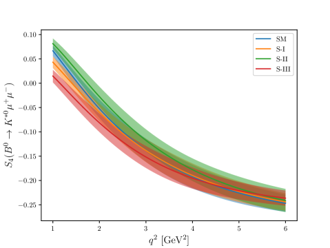
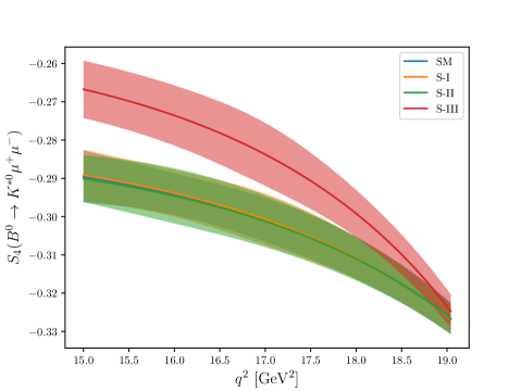
Figure 1: Plots of $S_{3,4,5}(q^{2})$ as a function of $q^{2}$ for SM and three NP scenarios. The left and right panels correspond to the low ($[1.1,6.0]$ GeV²) and high ($[15,19]$ GeV²) $q^{2}$ bins respectively. In each plot, the band represents the theoretical uncertainty mainly due to the form factors. Note that the scale on the y axis on each plot is different.

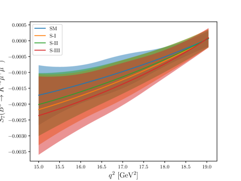
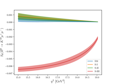
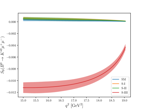
Figure 2: Plots of $S_{7,8,9}(q^{2})$ as a function of $q^{2}$ for SM and three NP scenarios. The left and right panels correspond to the low ($[1.1,6.0]$ GeV²) and high ($[15,19]$ GeV²) $q^{2}$ bins respectively. In each plot, the band represents the theoretical uncertainty mainly due to the form factors. Note that the scale on the y axis on each plot is different.

The longitudinal polarization fraction of $K^{*}$ depends on the distribution of the events in the angle $\theta_{K}$ (after integrating over $\theta_{\mu}$ and $\phi$) and the forward-backward asymmetry is defined in terms of $\theta_{\mu}$ (after integrating over $\theta_{K}$ and $\phi$). Both these quantities have very poor discrimination for NP other than scalar or tensor operators. Therefore, we study the observables that are based on the distribution in the azimuthal angle $\phi$. In particular, we investigate the distinguishing ability of $S_{3,4,5}$ and $S_{7,8,9}$. We compute the average values of these six observables for the SM and the three NP scenarios in four different $q^{2}$ bins, $q^{2}\subset[1.1,6.0],\,[15,17],\,[17,19]$ and $[15,19]$ GeV². These are listed in Tab 2. In this table, we also mention current measured values of these six quantities. We plot the six observables as a function of $q^{2}$ for the SM and the three NP scenarios. The $q^{2}$ plots for $S_{3,4,5}(q^{2})$ are shown in Fig. 1 whereas those for $S_{7,8,9}(q^{2})$ are given in Fig. 2. The average values and the plots are obtained by using Flavio package Straub:2018kue . This package uses the most precise form factor predictions obtained in light cone sum rule (LCSR) Straub:2015ica ; Gubernari:2018wyi approach, taking into account the correlations between the uncertainties of different form factors and at different values of $q^{2}$. The non-factorisable corrections are incorporated following the parameterization used in Ref. Straub:2015ica ; Straub:2018kue . These are also compatible with the calculations in Ref. Khodjamirian:2010vf .

Observable	$q^{2}$ bin	SM	S-I	S-II	S-III	Expt. value (LHCb)
	$[1.1,6]$	$-0.013\pm 0.005$	$-0.012\pm 0.005$	$-0.011\pm 0.005$	$-0.027\pm 0.007$	$-0.012\pm 0.025\pm 0.003$
$S_{3}$	$[15,17]$	$-0.173\pm 0.019$	$-0.173\pm 0.017$	$-0.173\pm 0.016$	$-0.124\pm 0.019$	$-0.166\pm 0.034\pm 0.007$
	$[17,19]$	$-0.251\pm 0.013$	$-0.252\pm 0.012$	$-0.252\pm 0.013$	$-0.220\pm 0.016$	$-0.250\pm 0.050\pm 0.025$
	$[15,19]$	$-0.205\pm 0.015$	$-0.205\pm 0.016$	$-0.205\pm 0.014$	$-0.162\pm 0.018$	$-0.189\pm 0.030\pm 0.009$
	$[1.1,6]$	$-0.147\pm 0.019$	$-0.147\pm 0.020$	$-0.130\pm 0.020$	$-0.159\pm 0.017$	$-0.136\pm 0.039\pm 0.003$
$S_{4}$	$[15,17]$	$-0.294\pm 0.006$	$-0.294\pm 0.006$	$-0.294\pm 0.007$	$-0.272\pm 0.007$	$-0.299\pm 0.033\pm 0.008$
	$[17,19]$	$-0.310\pm 0.006$	$-0.310\pm 0.006$	$-0.310\pm 0.006$	$-0.297\pm 0.006$	$-0.307\pm 0.041\pm 0.008$
	$[15,19]$	$-0.300\pm 0.006$	$-0.300\pm 0.007$	$-0.300\pm 0.006$	$-0.282\pm 0.007$	$-0.303\pm 0.024\pm 0.008$
	$[1.1,6]$	$-0.186\pm 0.037$	$-0.074\pm 0.046$	$-0.142\pm 0.042$	$-0.081\pm 0.055$	$-0.052\pm 0.034\pm 0.007$
$S_{5}$	$[15,17]$	$-0.318\pm 0.015$	$-0.288\pm 0.015$	$-0.316\pm 0.016$	$-0.324\pm 0.016$	$-0.341\pm 0.034\pm 0.009$
	$[17,19]$	$-0.226\pm 0.017$	$-0.205\pm 0.016$	$-0.224\pm 0.015$	$-0.237\pm 0.016$	$-0.280\pm 0.040\pm 0.014$
	$[15,19]$	$-0.280\pm 0.017$	$-0.254\pm 0.017$	$-0.278\pm 0.016$	$-0.289\pm 0.016$	$-0.317\pm 0.024\pm 0.011$
	$[1.1,6]$	$-0.019\pm 0.041$	$-0.023\pm 0.042$	$-0.022\pm 0.041$	$-0.025\pm 0.046$	$-0.090\pm 0.034\pm 0.002$
$S_{7}$	$[15,17]$	$-0.001\pm 0.001$	$-0.002\pm 0.001$	$-0.002\pm 0.001$	$-0.002\pm 0.001$	$0.029\pm 0.039\pm 0.001$
	$[17,19]$	$-0.001\pm 0.001$	$-0.001\pm 0.000$	$-0.001\pm 0.000$	$-0.001\pm 0.001$	$0.049\pm 0.049\pm 0.007$
	$[15,19]$	$-0.001\pm 0.001$	$-0.001\pm 0.001$	$-0.001\pm 0.001$	$-0.001\pm 0.001$	$0.035\pm 0.030\pm 0.003$
	$[1.1,6]$	$-0.006\pm 0.014$	$-0.004\pm 0.013$	$-0.006\pm 0.015$	$-0.003\pm 0.007$	$-0.009\pm 0.037\pm 0.002$
$S_{8}$	$[15,17]$	$0.000\pm 0.000$	$0.000\pm 0.000$	$0.000\pm 0.000$	$-0.006\pm 0.001$	$0.003\pm 0.042\pm 0.002$
	$[17,19]$	$0.000\pm 0.000$	$0.000\pm 0.000$	$0.000\pm 0.000$	$-0.005\pm 0.001$	$-0.026\pm 0.046\pm 0.002$
	$[15,19]$	$0.000\pm 0.000$	$0.000\pm 0.000$	$0.000\pm 0.000$	$-0.006\pm 0.001$	$0.005\pm 0.031\pm 0.001$
	$[1.1,6]$	$-0.001\pm 0.002$	$-0.001\pm 0.003$	$-0.001\pm 0.003$	$0.002\pm 0.005$	$-0.025\pm 0.026\pm 0.002$
$S_{9}$	$[15,17]$	$0.000\pm 0.000$	$0.001\pm 0.000$	$0.000\pm 0.000$	$-0.012\pm 0.001$	$0.000\pm 0.037\pm 0.002$
	$[17,19]$	$0.000\pm 0.000$	$0.000\pm 0.000$	$0.000\pm 0.000$	$-0.010\pm 0.001$	$-0.056\pm 0.045\pm 0.002$
	$[15,19]$	$0.000\pm 0.000$	$0.000\pm 0.000$	$0.000\pm 0.000$	$-0.012\pm 0.001$	$-0.031\pm 0.029\pm 0.001$

Table 2: Average values of $S_{3,4,5}$ and $S_{7,8,9}$ in four $q^{2}$ bins for the SM and three NP scenarios listed in Tab 1. Present experimental measurements of these quantities are also listed for comparison Aaij:2020nrf .

From the Figs. 1, 2 and Tab 2, we make following observations:

• The values of $S_{i}^{(a)}$ in the low-$q^{2}$ bin are lower compared to the values in the high-$q^{2}$ bin. The values of the observables $S_{3,4,5,7,8,9}$ in the low-$q^{2}$ bin do not have any ability to discriminate between three NP scenarios.

• In high $q^{2}$ bin, the $S_{5}$ and $S_{7}$ do not have any kind of discrimination power, whereas $S_{4}$ has a poor distinguishing capability for the NP scenario III. In addition, $S_{8}$ can also discriminate the third scenario, but the average values are less than $1\%$. Therefore, $S_{4}$ and $S_{8}$ are poor distinguishing tools.

• The prediction of NP scenario III and that of NP scenario I, for $S_{3}$ in high-$q^{2}$ bin, differ from each other by about $20\%$. But these predictions have a theoretical uncertainty of $10\%$. This observable becomes an effective distinguishing tool if the theoretical uncertainty can be reduced to $5\%$ and if the experimental uncertainty can also be reduced to a similar level.

• It is advantageous to use $S_{9}$ as a discriminator for NP scenario III because its theoretical uncertainty is negligibly small. NP scenario III predicts the value of $S_{9}$ in the high $q^{2}$ bin to be about a percent, whereas the predictions of the other two NP scenarios are zero. Measuring $S_{9}$ to a precision of $0.5\%$ leads to a $1\sigma$ distinction between NP scenario III from the other two. For $2\sigma$ distinction, the experimental uncertainty should be reduced by an additional factor of 2.

II.3 Measurement of $S_{3}$ and $S_{9}$ with the smallest possible uncertainty

The number of $B\to K^{*}\mu^{+}\mu^{-}$ events in an experiment are likely to be limited because of the very small branching ratio. If this small set of events is fitted to the full differential distribution in $q^{2}$ as well as in all the three angles $\theta_{K}$, $\theta_{\mu}$ and $\phi$ to determine $S_{i}^{(a)}(q^{2})$, the number of events in each bin will be rather small and the statistical uncertainties in such a determination will be quite large. It is possible to improve the statistics, by integrating over the polar angles $\theta_{K}$ and $\theta_{\mu}$ Bobeth:2008ij and define the two distributions

$$I_{\rm sum}(q^{2},\phi) = \int_{-1}^{1}d\cos\theta_{K}\int_{-1}^{1}d\cos\theta_{\mu}\left[I(q^{2},\theta_{K},\theta_{\mu},\phi)+\bar{I}(q^{2},\theta_{K},\theta_{\mu},\phi)\right]\,$$

$$I_{\rm diff}(q^{2},\phi) = \int_{-1}^{1}d\cos\theta_{K}\int_{-1}^{1}d\cos\theta_{\mu}\left[I(q^{2},\theta_{K},\theta_{\mu},\phi)-\bar{I}(q^{2},\theta_{K},\theta_{\mu},\phi)\right].$$ (12)

By doing a fit of $I_{\rm sum}(q^{2},\phi)$ and $I_{\rm diff}(q^{2},\phi)$ data binned in angle $\phi$, it is possible to determine the coefficient of $\cos 2\phi$ $(S_{3})$ and of $\sin 2\phi$ $(S_{9})$. However, it also is possible to measure $S_{3}$ and $S_{9}$ by considering $I_{\rm sum}(q^{2},\phi)$ and $I_{\rm diff}(q^{2},\phi)$ in $90^{\circ}$ wide bins of $\phi$ and define the two asymmetries

$$A_{3}(q^{2})=\frac{\left(\int^{\pi/4}_{-\pi/4}-\int^{3\pi/4}_{\pi/4}+\int^{5\pi/4}_{3\pi/4}-\int^{7\pi/4}_{5\pi/4}\right)d\phi I_{\rm sum}(q^{2},\phi)}{\left(\int^{\pi/4}_{-\pi/4}+\int^{3\pi/4}_{\pi/4}+\int^{5\pi/4}_{3\pi/4}+\int^{7\pi/4}_{5\pi/4}\right)d\phi I_{\rm sum}(q^{2},\phi)},$$ (13)

and Mandal:2014kma

$$A_{9}(q^{2})=\frac{\left(\int^{\pi/2}_{0}-\int^{\pi}_{\pi/2}+\int^{3\pi/2}_{\pi}-\int^{2\pi}_{3\pi/2}\right)d\phi I_{\rm diff}(q^{2},\phi)}{\left(\int^{\pi/2}_{0}+\int^{\pi}_{\pi/2}+\int^{3\pi/2}_{\pi}+\int^{2\pi}_{3\pi/2}\right)d\phi I_{\rm sum}(q^{2},\phi)}.$$ (14)

It is straight forward to show that $A_{3}=(2/\pi)S_{3}$ and $A_{9}=(2/\pi)S_{9}$. Since $A_{3}$ and $A_{9}$ are defined using the largest possible bins in $\phi$, they can be measured with the least possible statistical uncertainty. As discussed above, a determination of $A_{9}$, with low statistical error in the high $q^{2}$ bins, will lead to a clear distinction between the NP scenarios I and III.

III Conclusions

The global fits of the current data on the semi-leptonic $b\to s$ transitions lead to three different NP solutions (I) $C_{9}^{\rm NP}<0$, (II) $C_{9}^{\rm NP}=-C_{10}^{\rm NP}$, (III) $C_{9}^{\rm NP}=-C_{9}^{\prime\rm NP}$. In this work, we suggest a method to uniquely determine which of these three solutions is the correct one by investigating $B_{s}\to\mu^{+}\mu^{-}$ and $B\to K^{*}\mu^{+}\mu^{-}$ decays. The $B_{s}\to\mu^{+}\mu^{-}$ amplitude is non-zero only if the leptonic current has an axial-vector component. Among the three solutions, only scenario II satisfies this constraint. Therefore, the branching ratio of this decay can distinguish scenario II from the other two, provided the present experimental uncertainty in its measurement is reduced by a factor of three. It is expected that the Run-3 of LHC will lead to such a precise measurement Cerri:2018ypt . To make a distinction between the other two scenarios, we study the azimuthal angular observables in the decay $B\to K^{*}\mu^{+}\mu^{-}$ and show that the observables $S_{9}$ in high $q^{2}$ bin is an effective tool to distinguish between the NP scenarios I and III, provided its uncertainty is small enough. We also define an asymmetry in the azimuthal angle $\phi$, $A_{9}=(2/\pi)S_{9}$. This is directly measurable and utilizes the largest possible bin sizes in $\phi$. So, for any given data set, determination of $S_{9}$ through a measurement of $A_{9}$ leads to the smallest statistical uncertainty. Thus $A_{9}$ is a good tool to make a discrimination between scenarios I and III.

Data Availability Statement

This manuscript has no associated data. We have not used any data file in this work which has to be deposited.

Appendix A Angular coefficients

The angular coefficients in eq (9) can be expressed in terms of transversity amplitudes which are given by Altmannshofer:2008dz

$$I_{1}^{s} = \frac{(2+\beta^{2}_{\mu})}{4}\left[|A^{L}_{\perp}|^{2}+|A^{L}_{\parallel}|^{2}+(L\to R)\right]+\frac{4m^{2}_{\mu}}{q^{2}}{\rm Re}\left(A^{L}_{\perp}A^{R*}_{\perp}+A^{L}_{\parallel}A^{R*}_{\parallel}\right),$$

$$I^{c}_{1} = |A^{L}_{0}|^{2}+|A^{R}_{0}|^{2}+\frac{4m^{2}_{\mu}}{q^{2}}\left[|A_{t}|^{2}+2{\rm Re}\left(A^{L}_{0}A^{R*}_{0}\right)\right]+\beta^{2}_{\mu}|A_{S}|^{2},$$

$$I_{2}^{s} = \frac{\beta^{2}_{\mu}}{4}\left[|A^{L}_{\perp}|^{2}+|A^{L}_{\parallel}|^{2}+(L\to R)\right],$$

$$I^{c}_{2} = -\beta^{2}_{\mu}\left[|A^{L}_{0}|^{2}+|A^{R}_{0}|^{2}\right],$$

$$I_{3} = \frac{\beta^{2}_{\mu}}{2}\left[|A^{L}_{\perp}|^{2}-|A^{L}_{\parallel}|^{2}+(L\to R)\right],$$

$$I_{4} = \frac{\beta^{2}_{\mu}}{\sqrt{2}}\left[{\rm Re}(A^{L}_{0}A^{L*}_{\parallel})+(L\to R)\right],$$

$$I_{5} = \sqrt{2}\beta_{\mu}\left[{\rm Re}(A^{L}_{0}A^{L*}_{\perp})-(L\to R)-\frac{m_{\mu}}{\sqrt{q^{2}}}{\rm Re}(A^{L}_{\parallel}A^{*}_{S}+A^{R}_{\parallel}A^{*}_{S})\right],$$

$$I^{s}_{6} = 2\beta_{\mu}\left[{\rm Re}(A^{L}_{\parallel}A^{L*}_{\perp})-(L\to R)\right],$$

$$I^{c}_{6} = 4\beta_{\mu}\frac{m_{\mu}}{\sqrt{q^{2}}}{\rm Re}\left[A^{L}_{0}A^{*}_{S}+(L\to R)\right],$$

$$I_{7} = \sqrt{2}\beta_{\mu}\left[{\rm Im}(A^{L}_{0}A^{L*}_{\parallel})-(L\to R)+\frac{m_{\mu}}{\sqrt{q^{2}}}{\rm Im}(A^{L}_{\perp}A^{*}_{S}+A^{R}_{\perp}A^{*}_{S})\right],$$

$$I_{8} = \frac{\beta^{2}_{\mu}}{\sqrt{2}}\left[{\rm Im}(A^{L}_{0}A^{L*}_{\perp})+(L\to R)\right],$$

$$I_{9} = \beta^{2}_{\mu}\left[{\rm Im}(A^{L*}_{\parallel}A^{L}_{\perp})+(L\to R)\right].$$ (15)

The transversity amplitudes are written as

$$A_{\perp L,R} = N\sqrt{2\lambda}\left[\left[(C^{\rm eff}_{9}+C^{\rm eff\prime}_{9})\mp(C_{10}+C^{\prime}_{10})\right]\frac{V(q^{2})}{m_{B}+m_{K^{*}}}+\frac{2m_{b}}{q^{2}}C^{\rm eff}_{7}T_{1}(q^{2})\right],$$

$$A_{\parallel L,R} = -N\sqrt{2}(m^{2}_{B}-m^{2}_{K^{*}})\left[\left[(C^{\rm eff}_{9}-C^{\rm eff\prime}_{9})\mp(C_{10}-C^{\prime}_{10})\right]\frac{A_{1}(q^{2})}{m_{B}-m_{K^{*}}}+\frac{2m_{b}}{q^{2}}C^{\rm eff}_{7}T_{2}(q^{2})\right],$$

$$A_{0L,R} = -\frac{N}{2m_{K^{*}}\sqrt{q^{2}}}\left[[(C^{\rm eff}_{9}-C^{\rm eff\prime}_{9})\mp(C_{10}-C^{\prime}_{10})]\right.$$

$$\left\{(m^{2}_{B}-m^{2}_{K^{*}}-q^{2})(m_{B}+m_{K^{*}})A_{1}(q^{2})-\lambda\frac{A_{2}(q^{2})}{m_{B}+m_{K^{*}}}\right\}$$

$$\left.+2m_{b}C^{\rm eff}_{7}\left\{(m^{2}_{B}+3m^{2}_{K^{*}}-q^{2})T_{2}(q^{2})-\frac{\lambda}{m^{2}_{B}-m^{2}_{K^{*}}}T_{3}(q^{2})\right\}\right],$$

$$A_{t} = \frac{N}{\sqrt{q^{2}}}\sqrt{\lambda}\left[2(C_{10}-C^{\prime}_{10})+\frac{q^{2}}{m_{\mu}}(C_{P}-C^{\prime}_{P})\right]A_{0}(q^{2}),$$

$$A_{S} = -2N\sqrt{\lambda}(C_{S}-C^{\prime}_{S})A_{0}(q^{2}),$$ (16)

where

$$N=V_{tb}V^{*}_{ts}\left[\frac{G^{2}_{F}\alpha^{2}}{3.2^{10}\pi^{5}m^{3}_{B}}q^{2}\sqrt{\lambda}\beta_{\mu}\right]^{1/2},$$ (17)

with $\lambda=m^{4}_{B}+m^{4}_{K^{*}}+q^{4}-2(m^{2}_{B}m^{2}_{K^{*}}+m^{2}_{B}q^{2}+m^{2}_{K^{*}}q^{2})$ and $\beta_{\mu}=\sqrt{1-4m^{2}_{\mu}/q^{2}}$. The expressions of form-factors $V(q^{2})$, $A_{0,1,2}(q^{2})$ and $T_{1,2,3}(q^{2})$ can be found in ref. Straub:2015ica which are calculated by a combined fit of Light Cone Sum Rule and lattice QCD approaches.

References

• (1) R. Aaij et al. [LHCb Collaboration], JHEP 1708, 055 (2017) [arXiv:1705.05802 [hep-ex]].
• (2) R. Aaij et al. [LHCb Collaboration], Phys. Rev. Lett.  122, no. 19, 191801 (2019) [arXiv:1903.09252 [hep-ex]].
• (3) A. Abdesselam et al. [Belle], [arXiv:1904.02440 [hep-ex]].
• (4) R. Aaij et al. [LHCb], [arXiv:2103.11769 [hep-ex]].
• (5) G. Hiller and F. Kruger, Phys. Rev. D 69, 074020 (2004) [hep-ph/0310219].
• (6) M. Bordone, G. Isidori and A. Pattori, Eur. Phys. J. C 76, no. 8, 440 (2016) [arXiv:1605.07633 [hep-ph]].
• (7) R. Aaij et al. [LHCb Collaboration], JHEP 1509, 179 (2015) [arXiv:1506.08777 [hep-ex]].
• (8) R. Aaij et al. [LHCb Collaboration], Phys. Rev. Lett.  111, 191801 (2013) [arXiv:1308.1707 [hep-ex]].
• (9) R. Aaij et al. [LHCb Collaboration], JHEP 1602, 104 (2016) [arXiv:1512.04442 [hep-ex]].
• (10) R. Aaij et al. [LHCb], Phys. Rev. Lett. 125 (2020) no.1, 011802 [arXiv:2003.04831 [hep-ex]].
• (11) S. Descotes-Genon, T. Hurth, J. Matias and J. Virto, JHEP 1305, 137 (2013) [arXiv:1303.5794 [hep-ph]].
• (12) M. Algueró, B. Capdevila, A. Crivellin, S. Descotes-Genon, P. Masjuan, J. Matias and J. Virto, Eur. Phys. J. C 79 (2019) no.8, 714 [arXiv:1903.09578 [hep-ph]].
• (13) A. K. Alok, A. Dighe, S. Gangal and D. Kumar, JHEP 1906, 089 (2019) [arXiv:1903.09617 [hep-ph]].
• (14) M. Ciuchini, A. M. Coutinho, M. Fedele, E. Franco, A. Paul, L. Silvestrini and M. Valli, Eur. Phys. J. C 79 (2019) no.8, 719 [arXiv:1903.09632 [hep-ph]].
• (15) G. D’Amico, M. Nardecchia, P. Panci, F. Sannino, A. Strumia, R. Torre and A. Urbano, JHEP 1709, 010 (2017) [arXiv:1704.05438 [hep-ph]].
• (16) A. Datta, J. Kumar and D. London, Phys. Lett. B 797 (2019) 134858 [arXiv:1903.10086 [hep-ph]].
• (17) J. Aebischer, W. Altmannshofer, D. Guadagnoli, M. Reboud, P. Stangl and D. M. Straub, arXiv:1903.10434 [hep-ph].
• (18) K. Kowalska, D. Kumar and E. M. Sessolo, Eur. Phys. J. C 79, no. 10, 840 (2019) [arXiv:1903.10932 [hep-ph]].
• (19) A. Arbey, T. Hurth, F. Mahmoudi, D. M. Santos and S. Neshatpour, Phys. Rev. D 100, no. 1, 015045 (2019) [arXiv:1904.08399 [hep-ph]].
• (20) L. S. Geng, B. Grinstein, S. Jager, S. Y. Li, J. Martin Camalich and R. X. Shi, [arXiv:2103.12738 [hep-ph]].
• (21) W. Altmannshofer and P. Stangl, [arXiv:2103.13370 [hep-ph]].
• (22) T. Hurth, F. Mahmoudi, D. M. Santos and S. Neshatpour, [arXiv:2104.10058 [hep-ph]].
• (23) A. Carvunis, F. Dettori, S. Gangal, D. Guadagnoli and C. Normand, [arXiv:2102.13390 [hep-ph]].
• (24) B. Grinstein and J. Martin Camalich, Phys. Rev. Lett.  116, no. 14, 141801 (2016) [arXiv:1509.05049 [hep-ph]].
• (25) D. Kumar, J. Saini, S. Gangal and S. B. Das, Phys. Rev. D 97, no. 3, 035007 (2018) [arXiv:1711.01989 [hep-ph]].
• (26) S. Kumbhakar and J. Saini, Eur. Phys. J. C 79, no. 5, 394 (2019) [arXiv:1807.04055 [hep-ph]].
• (27) D. Guadagnoli, M. Reboud and R. Zwicky, JHEP 1711, 184 (2017) [arXiv:1708.02649 [hep-ph]].
• (28) G. Abbas, A. K. Alok and S. Gangal, arXiv:1805.02265 [hep-ph].
• (29) Y. Amhis, S. Descotes-Genon, C. Marin Benito, M. Novoa-Brunet and M. H. Schune, [arXiv:2005.09602 [hep-ph]].
• (30) U. Egede, T. Hurth, J. Matias, M. Ramon and W. Reece, JHEP 11, 032 (2008) [arXiv:0807.2589 [hep-ph]].
• (31) U. Egede, T. Hurth, J. Matias, M. Ramon and W. Reece, JHEP 10, 056 (2010) [arXiv:1005.0571 [hep-ph]].
• (32) B. Capdevila, S. Descotes-Genon, J. Matias and J. Virto, JHEP 10, 075 (2016) [arXiv:1605.03156 [hep-ph]]
• (33) M. Algueró, B. Capdevila, S. Descotes-Genon, P. Masjuan and J. Matias, JHEP 07, 096 (2019) [arXiv:1902.04900 [hep-ph]].
• (34) J. Kumar and D. London, Phys. Rev. D 99 (2019) no.7, 073008 [arXiv:1901.04516 [hep-ph]].
• (35) A. K. Alok, S. Kumbhakar, J. Saini and S. U. Sankar, Nucl. Phys. B 967 (2021), 115419 [arXiv:2011.14668 [hep-ph]].
• (36) A. K. Alok, D. Kumar, S. Kumbhakar and S. U. Sankar, Phys. Rev. D 95 (2017) no.11, 115038 [arXiv:1606.03164 [hep-ph]].
• (37) S. Bhattacharya, S. Nandi and S. Kumar Patra, Eur. Phys. J. C 79 (2019) no.3, 268 [arXiv:1805.08222 [hep-ph]].
• (38) A. K. Alok, D. Kumar, S. Kumbhakar and S. Uma Sankar, Phys. Lett. B 784 (2018), 16-20 [arXiv:1804.08078 [hep-ph]].
• (39) Z. R. Huang, Y. Li, C. D. Lu, M. A. Paracha and C. Wang, Phys. Rev. D 98 (2018) no.9, 095018 [arXiv:1808.03565 [hep-ph]].
• (40) A. K. Alok, D. Kumar, S. Kumbhakar and S. Uma Sankar, Nucl. Phys. B 953 (2020), 114957 [arXiv:1903.10486 [hep-ph]].
• (41) C. Murgui, A. Peñuelas, M. Jung and A. Pich, JHEP 09 (2019), 103 [arXiv:1904.09311 [hep-ph]].
• (42) R. X. Shi, L. S. Geng, B. Grinstein, S. Jäger and J. Martin Camalich, JHEP 12 (2019), 065 [arXiv:1905.08498 [hep-ph]].
• (43) M. Blanke, A. Crivellin, T. Kitahara, M. Moscati, U. Nierste and I. Nisandzic, [arXiv:1905.08253 [hep-ph]].
• (44) P. Asadi and D. Shih, Phys. Rev. D 100 (2019) no.11, 115013 [arXiv:1905.03311 [hep-ph]].
• (45) S. Aoki et al. [Flavour Lattice Averaging Group], Eur. Phys. J. C 80 (2020) no.2, 113 [arXiv:1902.08191 [hep-lat]].
• (46) M. Tanabashi et al. [Particle Data Group], Phys. Rev. D 98 (2018) no.3, 030001
• (47) D. M. Straub, [arXiv:1810.08132 [hep-ph]].
• (48) M. Beneke, C. Bobeth and R. Szafron, JHEP 10 (2019), 232 [arXiv:1908.07011 [hep-ph]].
• (49) A. Cerri, V. V. Gligorov, S. Malvezzi, J. Martin Camalich, J. Zupan, S. Akar, J. Alimena, B. C. Allanach, W. Altmannshofer and L. Anderlini, et al. CERN Yellow Rep. Monogr. 7 (2019), 867-1158 [arXiv:1812.07638 [hep-ph]].
• (50) R. Aaij et al. [LHCb], [arXiv:1808.08865 [hep-ex]].
• (51) C. Bobeth, G. Hiller and G. Piranishvili, JHEP 07 (2008), 106 [arXiv:0805.2525 [hep-ph]].
• (52) W. Altmannshofer, P. Ball, A. Bharucha, A. J. Buras, D. M. Straub and M. Wick, JHEP 0901, 019 (2009) [arXiv:0811.1214 [hep-ph]].
• (53) N. Gubernari, A. Kokulu and D. van Dyk, JHEP 1901 (2019) 150 [arXiv:1811.00983 [hep-ph]].
• (54) A. Bharucha, D. M. Straub and R. Zwicky, JHEP 1608, 098 (2016) [arXiv:1503.05534 [hep-ph]].
• (55) A. Khodjamirian, T. Mannel, A. A. Pivovarov and Y.-M. Wang, JHEP 1009, 089 (2010) [arXiv:1006.4945 [hep-ph]].
• (56) R. Mandal, R. Sinha and D. Das, Phys. Rev. D 90 (2014) no.9, 096006 [arXiv:1409.3088 [hep-ph]].