Many-body electronic structure of LaScO₃ by real space quantum Monte Carlo

Abstract

We present real space quantum Monte Carlo (QMC) calculations of the scandate LaScO₃ that proved to be challenging for traditional electronic structure approaches due to strong correlation effects resulting in inaccurate band gaps from DFT and $GW$ methods when compared with existing experimental data. Besides calculating an accurate QMC band gap corrected for supercell size biases and in agreement with numerous experiments, we also predict the cohesive energy of the crystal using the standard fixed-node QMC without any empirical or non-variational parameters. We show that promotion (optical) gap and fundamental gap agree with each other illustrating a clear absence of significant excitonic effects in the ideal crystal. We obtained these results in perfect consistency in two independent tracks that employ different basis sets (plane wave vs. localized gaussians), different codes for generating orbitals (Quantum Espresso vs. Crystal), different QMC codes (Qmcpack vs. Qwalk) and different high-accuracy pseudopotentials (ccECPs vs. Troullier-Martins) presenting the maturity and consistency of QMC methodology and tools for studies of strongly correlated problems.

PACS numbers

May be entered using the \pacs{#1} command.

I Introduction

Transition metal oxides that crystalize in perovskite structures are intensely studied materials due to their complex many-body effects as well as for their potential for broad applications. The challenges in understanding their electronic properties are well-known and include electron-electron correlation, competition of localized $d$ vs. more extended $s$ and $p$ states, crystal field effects, and spin-orbit contributions for heavier elements. A number of studies over the decades have been devoted to understand these effects within a range of approaches such as density functional theory (DFT), post-DFT, and dynamical mean-field theory (DMFT). Very recently, a group of La-based perovskites with formula LaMO₃ where M represents a $3d$ transition metal Pari et al. (1995); He and Franchini (2012); Ergönenc et al. (2018); Santana et al. (2017) have proved to be rather challenging even for the most advanced methods. Most of these La-based crystals show local magnetic moments and magnetic orderings as is often the case for transition element perovskites with partially filled shells, especially for the middle/late $3d$ series. Interestingly, the scandate LaScO₃ is rather atypical since the scandium $d$-shell becomes nominally empty and the ground state therefore appears to be nonmagnetic. The La atom contributes charge towards closing the empty shells of oxygens and stabilizes the structure by filling the empty space between the ScO₆ octahedra in the typical perovskite arrangement and results in a large gap, as determined by various optical experiments Afanas’ev et al. (2004); Arima et al. (1993); Heeg et al. (2006). Seemingly, its electronic structure should be not much different from other nonmagnetic closed-shell perovskites that have been described with a mixed degree of accuracy by a variety of post-DFT approaches such as $GW$, DFT+$U$, and more elaborate DMFT methods. It is therefore somewhat unexpected that this system proved to be difficult to reconcile with available experimental data, since the gap estimations are smaller than experiments by 1 eV or more, even in post-DFT methods. As explained by Millis et al Dang et al. (2014), the arbitrary boost to Hubbard $U$, which is often used as a fix for ordinary DFT methods to open the gap in transition metal oxides, is not helpful since the $d$-levels are nominally unoccupied. Indeed, ad hoc, educated double-counting schemes adapted for DFT+DMFT had to be employed in order to build the theoretical understanding of experimental gaps so that a proper balance of the charge-transfer vs. Mott-like behavior is reached in related systems such as LaTiO₃ Dang et al. (2014). Alternative methods such as $GW$ show somewhat mixed success for this class of systems. In a systematic and very precise study with several variants of the $GW$ approach Ergönenc et al. (2018), heavier transition metal oxide gaps agree quite well with the experiment, whereas in LaTiO₃, the gap is overestimated by $\sim 0.9$ eV. On the other hand for LaScO₃, the study shows an underestimated gap by $\sim 1-1.5$ eV, depending on the details of the $GW$ method. For LaScO₃ in particular, the resulting discrepancy has led to the claim that the $GW$ result is more reliable than the experiment in this case, despite numerous optical studies indicating the gap is at least as large as 5.7 eV, and quite possibly larger. Considering these contradictions, here we present an independent many-body study of LaScO₃ system using real space quantum Monte Carlo which has paved the way for employing correlated wave function electronic structure methods to real materials with strong correlations over the last two decades. We find agreement with the experimental band gap without any empirical inputs or ad hoc parameter tuning, merely using the fixed-node diffusion Monte Carlo (FNDMC) approach in its variational formulation, and corroborate our result with two independent QMC codes. We probe the band gap using the canonical definition as well as optical promotion excitation with the same results. We also propose a method for analysis and correction of finite size effects for the band gap estimation with increasing supercell sizes. In addition, we predict the value of the crystal cohesion energy, for which to the best of our knowledge there is no experimental determination. Therefore, this represents a genuine prediction from our many-body methods. In addition, we find that despite being a strongly correlated system, LaScO₃ is very well described by a single-reference wave function nodal surface with corresponding correlations recovered by the ordinary DMC method leading to accurate energy differences.

II Methods

ABO₃ perovskites, with A, B as cations and O being the anion, can crystallize in a variety of crystal symmetries. LaScO₃ in particular crystallizes with the $Pnma(62)$ crystal symmetry. Oxygen anions surround the Sc cations to form ScO₆ octahedra, while the La cations fill the space between these octahedra and close the O $p$ shell. Since Sc⁺³ and La⁺³ are closed-shell, LaScO₃ is nonmagnetic as opposed to other LaBO₃ perovskites, where the partially filled $d$ shells facilitate G-type anti-ferromagnetism. The experimental structural information is given in Table 1 and illustrated in Fig. 1. We note that while the previous DFT and post-DFT calculations that we will be comparing to have used a slightly different experimental structure Geller (1957), we use a more recent experimental determination of the structure Clark et al. (1978). The difference between these experimental structures results in only a 0.05% difference in the volumes and less than 1% error for the various Sc-O octahedral bonds. Hybrid DFT studies with HSE06 find that the DFT relaxed structures all have similar percent errors to the older experimental structure, and that the band gap is sensitive to at most 0.1 eV between the experimental and relaxed geometries He and Franchini (2012). Therefore, while all calculations considered in this work use the more recent experimental geometry, any comparison to DFT and post-DFT methods that use the older experimental geometries would change the differences only marginally, within approximately 0.1 eV, if our adopted geometry had been used.

Table 1: Experimental structure for LaScO₃ in the $Pnma(62)$ crystal structure Clark et al. (1978).

Lattice Parameters		$a$ (Å)	$b$ (Å)	$c$ (Å)
		5.7911	8.0923	5.6748
Atom	Site	$x$	$y$	$z$
O1	8$d$	0.1988	0.0528	0.3044
O2	4$c$	0.43745	1/4	0.01537
La	4$c$	0.5323	1/4	0.5996
Sc	4$a$	0	0	0

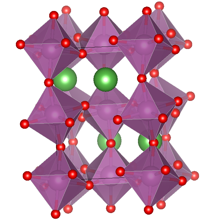
Figure 1: LaScO₃ in the experimental perovskite structure. ScO₆ octahedra are shown in purple, with the O atoms shown in red. The La⁺³ cations are shown in green. This figure was generated using the VESTA software Momma and Izumi (2011).

As opposed to effective Hamiltonian methods like DFT, DFT+$U$, DFT+$GW$, DFT+DMFT, etc., diffusion Monte Carlo (DMC) works directly with the many-body wave function. Using the imaginary time Schrödinger equation, we apply an imaginary time evolution operator to a trial wave function $e^{-\tau H}\Psi_{T}$ which evolves to the ground state in the long time evolution limit. Although this is formally exact, in order to deal with the fermion sign problem, we employ the well-known fixed-node approximation (FNDMC) Foulkes et al. (2001). In this approximation, the obtained solution is enforced to have the same zero/nodal surface as the trial wave function. This amounts to adding an additional term to the Hamiltonian, $H\rightarrow H+V_{\infty}\delta(\mathbf{R}-\mathbf{R}_{\partial\Omega})$, where $\mathbf{R}_{\partial\Omega}=\left\{\mathbf{R};\Psi_{T}(\mathbf{R})=0\right\}$ while $\mathbf{R}$ denotes coordinates of all involved electrons. The strength of the interaction is such that $V_{\infty}\to\infty$, so that it enforces a zero boundary condition at the trial nodal surface Melton and Mitas (2017). Since a non-exact nodal surface can only raise the energy relative to the exact energy, the expectation value of such Hamiltonian is therefore variational.

The accuracy of the method clearly relies on the accuracy of the trial wave function. Throughout this work, we utilize a Slater-Jastrow wave function

$$\Psi_{T}(\mathbf{R})=e^{J(\mathbf{R})}D_{\uparrow}(\psi_{k}^{\uparrow}(\mathbf{r}_{i}))D_{\downarrow}(\psi_{l}^{\downarrow}(\mathbf{r}_{j}))\,.$$ (1)

Here, $D_{\sigma}$ is a Slater determinant for spin $\sigma$ and $\psi_{i}^{\sigma}(\mathbf{r}_{j})$ form the single-particle orbital matrix. The Jastrow factor $J(\mathbf{R})$ builds explicit correlation into the trial wave function by considering electron-electron, electron-ion, and electron-electron-ion terms; clearly, the Jastrow cannot modify the nodal surface. In order to carry out a restricted optimization of the nodal surface, we use various sets of single-particle orbitals obtained from Hartree-Fock (HF), LDA, and PBE0_w where $w$ determines the amount of exact exchange in PBE0, defined as

$${\rm PBE0}_{w}=wE^{\rm HF}_{\rm x}+(1-w)E^{\rm PBE}_{\rm x}+E^{\rm PBE}_{\rm c}\,.$$ (2)

For both the ground and excited state calculations considered, we optimize the Jastrow coefficients within variational Monte Carlo (VMC) using the linear method Umrigar et al. (2007), and take the lowest energy from FNDMC as the optimal nodal surface.

In order to estimate the gap within DMC, tradionally two approaches have been utilized, namely the quasiparticle and optical formulations Hunt et al. (2018); Yang et al. (2019); Frank et al. (2019). In the quasiparticle approach, the gap is estimated by considering electron addition/removal from the wave function. By considering the addition/removal of an electron from the valence band maximum (VBM) and the conduction band minimum (CBM), we directly target the fundamental gap of the material. It is given by the following difference of total energies for system with $(N\pm 1)$ and $N$ electrons

$$\Delta_{\rm qp} = E_{N+1}+E_{N-1}-2E_{N}$$

$$\Psi_{N-1} = c_{\rm VBM}\Psi_{N}$$

$$\Psi_{N+1} = c^{\dagger}_{\rm CBM}\Psi_{N}\,,$$ (3)

with $\Psi_{N(\pm 1)}$ being the eigenstate for the $N(\pm 1)$ electron systems. Since each addition/removal is intended to be the ground state of the respective $N\pm 1$ systems, the FNDMC variational theorem holds and we take the lowest energy nodal surface. An alternative method is to use the optical excitation approach, which is argued to target the optical gap instead of the fundamental gap, potentially including excitonic information due to the electron-hole interaction. This is achieved by promoting a particle to an excited state, typically from the valence band maximum to the conduction band minimum

$$\Delta_{\rm op} = E^{\rm ex}_{N}-E_{N}$$

$$\Psi_{N}^{\rm ex} = c^{\dagger}_{\rm CBM}c_{\rm VBM}\Psi_{N}\,,$$ (4)

where $\Psi^{\rm ex}$ is the wave function for the excited state system. Although in general, the fixed-node approximation is only variational for the ground state, often the change of symmetry from VBM to CBM state guarantees the orthogonality of the excitation and the variational bound. Even when both VBM and CBM are of the same symmetry, the nodal constraint is sufficiently restrictive that single-particle excitations results in variational behavior in practice Hunt et al. (2018), (see Foulkes et al. Foulkes et al. (1999) for possible exceptions). In some cases, the optical gap may not be adequately described by the single-particle excitation used in the optical approach and a more elaborated methodology to target excited states has been developed Zhao and Neuscamman (2019) for QMC methods; however, here we restrict ourselves to the common single particle-excitation due to the absence of any pronounced excitonic effects. In cases where the dielectric constant is large, excitonic effects are largely screened out, and thus the optical and quasiparticle approach are nominally equivalent. This should be indeed the case for LaScO₃ with a dielectric constant of $\epsilon\simeq 24$ Heeg et al. (2005), therefore we expect both approaches to produce equivalent results within the energy resolution of our QMC calculations.

In order to test the validity of our calculations, we utilize two independent QMC codes, namely Qwalk Wagner et al. (2009) and Qmcpack Kim et al. (2018). For the Qwalk calculations, we generate our trial wave functions using orbitals with localized gaussian basis sets with Crystal Dovesi et al. (2005, 2009). Gaussian orbital codes like Crystal are well-suited for semi-local effective core potentials, which allows us to use our recently generated correlation consistent effective core potentials (ccECPs) for Sc Annaberdiyev et al. (2018) and O Bennett et al. (2017), which are designed for explicitly correlated methods like FNDMC. Since at present a ccECP for La has not been constructed, we instead use an existing ECP from the Stuttgart group Dolg et al. (1989, 1993), which has been appropriately modified to remove the Coulomb singularity in the potential, without changing the properties of the potential or any energy differences. We generate basis sets of the TZDP quality for O^-1, La⁺² and Sc⁺², which are close to the realized oxidation states in LaScO₃. In order to utilize our ccECPs within Qmcpack, periodic boundary conditions are mostly supported by orbital generation from Quantum Espresso (QE) Giannozzi et al. (2009, 2017). This requires a transformation of our semi-local ccECPs to the non-local Kleinman-Bylander (KB) form Kleinman and Bylander (1982) for orbital generation, although the original semi-local pseudopotential is used in the actual QMC calculations. While this is an exact transformation for the reference state, in general the potential is different than the semi-local form and can introduce errors such as ghost states and/or compromised transferability in subsequent QMC calculations Drummond et al. (2016). We found that while our ccECPs for Sc and O did not result in ghost states, the Stuttgart group pseudopotential did, and therefore we utilized another pseudopotential for La designed in DFT that has been specifically adapted to to be used in Kleinman-Bylander (KB) form with plane wave basis set Rappe et al. (1990). We denote this La pseudopotential as dft-kb. By comparing Qmcpack and Qwalk calculations, we cross-check that quality of the KB transformation of our ccECP potentials for Sc and O. In addition, we also test another set of pseudopotentials for Sc and O designed for QMC calculations Krogel et al. (2016) which we denote as dft-opt and compare the results with our ccECPs using Qwalk.

III Results

III.1 Optimal nodal surfaces

First, we focus on finding optimal nodal surfaces using orbital sets generated by hybrid DFT function PBE0_w where $w$ denotes the weight of the exact exchange (the original PBE0 functional has $w=0.25$).

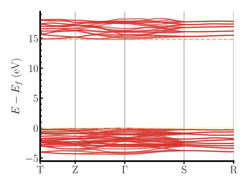
(a) HF

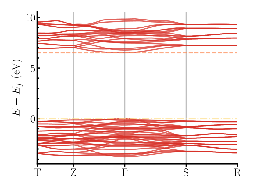
(b) PBE0

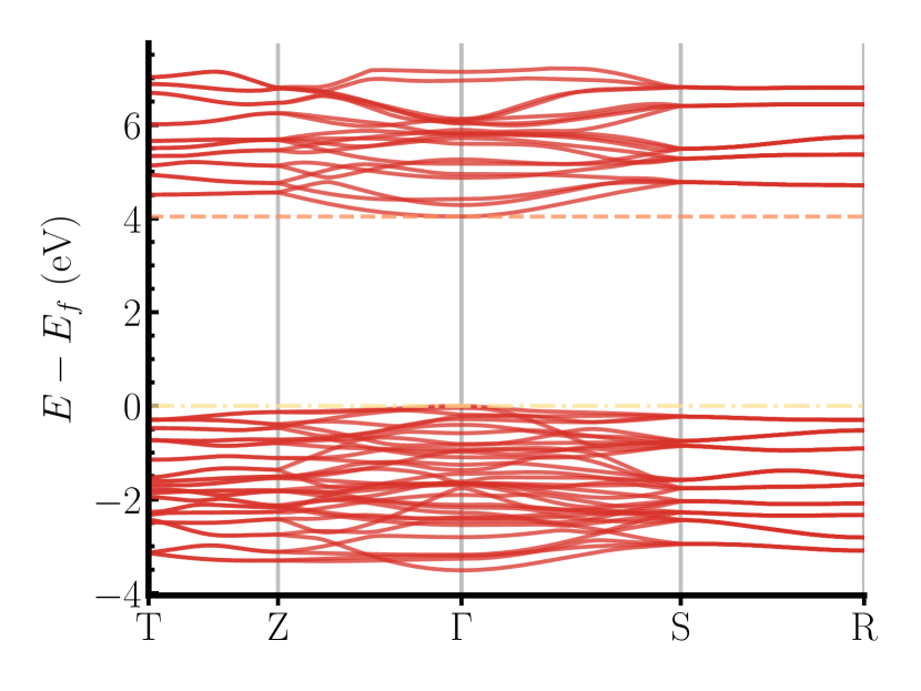
(c) PBE

Figure 2: LaScO₃ self-consistent band structures in the experimental geometry with varying degree of exact exchange. (2(a)) Hartree-Fock (HF) band structure gap of 14.82 eV is indirect with the valence band minimum (VBM) at $\Gamma$. However, the conduction band is very flat with a marginal difference between the precise conduction band minumum (CBM) and the $\Gamma$ point. (2(b)) The PBE0 band structure shows a direct gap of 6.51 eV at $\Gamma$. Similarly, (2(c)) the PBE band structure shows a direct gap of 4.04 eV at $\Gamma$.

In order to see the impact of nodal changes both on the ground and excited states, we probe the optical excitation where we simply promote an electron in the Slater determinant from VBM to CBM. For this purpose, we plot the one-particle band structures from Hartree-Fock (HF), PBE0 and PBE calculations in Fig. 2. The plot shows that the band extremes are both at the $\Gamma$ point in the range of $w$ where we expect the optimal mixing of the exact exchange $w$ that typically falls between 10 and 40% Wagner and Mitas (2003); Kolorenč et al. (2010).

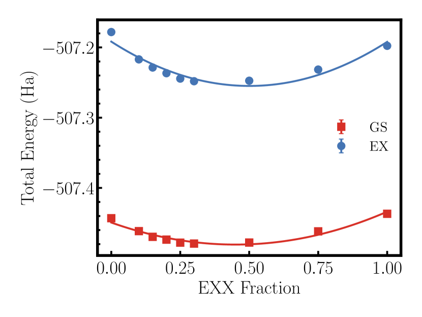
(a) FNDMC with ccECPs and dft-kb for La

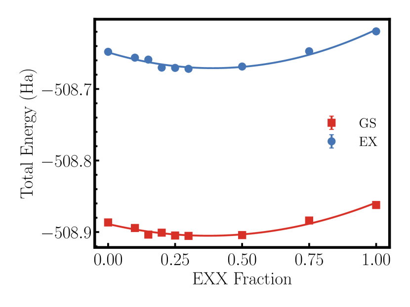
(b) FNDMC with dft-opt pseudopotentials

Figure 3: FNDMC total energies of LaScO₃ ground (squares) and excited (circles) states at the $\Gamma$ point plotted as functions of the exact exchange weight $w$. The corresponding orbital sets are generated by PBE0_w and FNDMC calculations are carried out using Qmcpack. Part (3(a)) uses ccECPs for Sc and O, and dft-kb pseudopotential for La Rappe et al. (1990). Part (3(b)) is calculated with dft-opt pseudopotentials Krogel et al. (2016).

In Fig. 3, we show the calculated ground and excited states from DMC using the QMCPACK code. These calculations use a 20-atom simulation cell, with 160 electrons, and we perform the ground state and excited state calculations with a $\Gamma$ point twist vector.

By mixing the hybrid exchange in the density functional used to generate the Slater part of the determinant, we are able to optimize the nodal surface for both the ground state and excited state. Fig. 3(a) shows the calculations using the ccECPs for Sc and O and dft-kb pseudopotential for La Ramer and Rappe (1999), whereas the Fig. 3(b) shows the same for the dft-opt pseudopotentials. Irrespective of the pseudopotentials used, the total energies for the ground and excited state have similar behavior. The minima occur around $w=0.3$ mixing although for the ground states PBE0 with $w=0.2,0.25$ are essentially identical by being basically within the error bar.

III.2 Cohesive Energy

In order to further test the quality of the softer dft-opt Krogel et al. (2016) pseudopotentials generated for use in QE and Qmcpack, we also directly compare the cohesive energies using two independent strands of calculations with different ECPs, basis sets and QMC codes. In particular, we utilize our ccECPs for Sc and O, Stuttgart ECP for La, in the Crystal code for generating the orbitals expanded in gaussian basis sets and running the FNDMC with Qwalk. The other independent track of calculations uses dft-opt pseudopotentials, Quantum Espresso with plane waves and FNDMC calculations carried out with Qmcpack. The atomic energies are calculated with single-reference fixed-node trial wave functions, and can be found in Table 2. These will be used as a reference when calculating the cohesive energy of LaScO₃.

We perform twist averaging to deal with the single-particle finite size effects, both with a variety of twist grids shown in Table 3. Each twist averaged calculation is carried out using the nodal surface generated by PBE0₂₅ nodes. We point out that if we consider the $\Gamma$ point only, we find excellent agreement between the cohesive energies of the two sets of results. This is quite encouraging, given the difference in orbital generation, QMC codes, effective Hamiltonians and different basis sets. In addition, as we converge the twist grids to the 4x4x4, we obtain again excellent agreement. The disagreement at intermediate twists in due to symmetry considerations when generating the one-particle orbitals. Given the agreement between the two QMC codes and various pseudopotentials, we focus on the Qwalk results for extrapolation to the thermodynamic limit. The extrapolation is used to filter out the two-body finite size effects and to this end, we perform a supercell calculation and extrapolate to the thermodynamic limit alongside the twist-averaging. The supercell is chosen such that it doubles the number of atoms and it is as close to a cube as possible. The cohesive energy per chemical formula is typically linearly extrapolated to the thermodynamic limit with scaling variable $1/N$ where $N$ is the number of formula units. The various cell energies are collected in Table 4. Note that already at 40 atom supercell the energy components are close to the twist averages. When extrapolated to the thermodynamic limit, they yield cohesive energy of 1.329 Ha per formula unit. To the best of our knowledge, there is no experimental cohesion available, and thus this is a genuine prediction.

Table 2: Atomic energies from fixed-node diffusion Monte Carlo and single reference single-reference trial wave functions. For the Qwalk calculations, we utilize our ccECPs and the dft-kb pseudopotential for La, while for the Qmcpack calculations here we use dft-opt pseudopotentials.

Atom	Qwalk/ccECP	Qmcpack/dft-opt
La	-31.40293(22)	-31.536684(4)
O	-15.86548(39)	-15.90088(27)
Sc	-46.52048(35)	-46.63115(48)

Table 3: Comparison of the twist-averaged energies for the 20-atom simulation cell between Qwalk and Qmcpack. The Qwalk calculations utilize the ccECPs (dft-kb for La), whereas the Qmcpack calculations are using dft-opt pseudopotentials. The corresponding atomic energies are in Table 2. Total energies are given per formula unit.

	Qwalk/ccECP		QMCPACK/opt
Twists	E (Ha)	Coh. (Ha)	E (Ha)	Coh. (Ha)
$\Gamma$	-126.87466(6)	1.3548(08)	-127.2262(04)	1.3558(08)
2x2x2	-126.8903(08)	1.3704(11)	-127.2568(08)	1.3864(10)
3x3x3	-126.8956(10)	1.3757(10)	-127.2546(04)	1.3841(07)
4x4x4	-126.9058(05)	1.3860(09)	-127.2556(02)	1.3851(07)

Table 4: Total, kinetic, and potential energies for the various Qwalk calculations. This includes two supercell sizes and several twist grids. Energies are given per formula unit.

$N_{\rm at}$	$k$-points	Energy	Kinetic	Potential
20	$\Gamma$	-126.87466(6)	65.493(17)	-207.492(07)
	2x2x2	-126.8903(08)	65.401(11)	-207.403(09)
	3x3x3	-126.8956(10)	65.373(11)	-207.380(09)
	4x4x4	-126.9058(05)	65.325(07)	-207.356(06)
40	$\Gamma$	-126.8729(4)	65.436(13)	-207.431(23)
	3x3x3	-126.8775(4)	65.380(12)	-207.363(13)

III.3 Band gap

We first discuss the band gap of LaScO₃, for both the experimental and DFT methods. From optical conductivity measurements, the spectral intensity shows a clear increase at $\approx$ 6 eV Arima et al. (1993). Numerous other optical measurements yield similar gaps. For example, a band gap of 5.7(1) eV for LaScO₃ was found from samples grown with molecular beam deposition and pulsed laser deposition Afanas’ev et al. (2004) as well as $>$ 5.8 eV using epitaxial films Heeg et al. (2006). From this, it is clear that the band gap is nearly 6.0 eV or perhaps slightly above, with an experimental uncertainty of a few tenths of eV. Previous LDA calculations underestimate the bandgap as 3.98 eV Ravindran et al. (2004), whereas PBE in the experimental structure has been found to be 3.81 eV He and Franchini (2012), which is clearly related to the well-known band gap underestimation in DFT. This is in close agreement with our independent PBE calculations, shown in Fig. 2(c), which gives a band gap of 4.04 eV. Note that although the settings are not identical since we employ different pseudopotentials, gaussian basis sets vs. plane wave basis sets, slightly different experimental geometries to the ones used previously and different codes, the results are very close. Additionally, we provide both HF and PBE0 band structures with 25% exact exchange, labeled as PBE0, which show the increase in the bandgap as exact exchange weight is increased as expected, with plots in Fig. 2. A similar behavior was demonstrated in He and Franchini (2012) using the HSE06 hybrid functional. Clearly, the band gap from the hybrid functional depends on the mixing and therefore it requires an educated guess and fine tuning in order to find proper effective exchange mixing.

In order to probe for the accuracy and impact of the nodal surface on the band gap, we first estimate the optical gap, with simple promotion of an electron in the Slater determinant from VBM to CBM, which are both at the $\Gamma$ point (Fig. 2). In Fig. 3, we show the calculated ground and excited states from fixed-node DMC using the QMCPACK code with total of 20 atoms in the simulation cell. By varying the Fock exchange in PBE0 functional, we generate orbitals for the Slater determinant and therefore scan the corresponding nodal surfaces for both the ground state and excited state Kolorenč et al. (2010). Fig. 3(a) shows the ground state and excited state calculations using the ccECPs for Sc and O and the dft-kb pseudopotential for La, whereas the Fig. 3(b) shows the ground state and excited state calculations using the softer dft-opt pseudopotentials. Irrespective of the pseudopotential sets used, the total energies for the ground and excited state show similar behavior. The minima of the DMC energy occurs using nodal surfaces of PBE0₃₀. From this, we can estimate the gap for each; the uncorrected gap using the ccECPs is 6.28(7) eV whereas using the designed QMC potentials we estimate 6.36(7) eV showing an excellent consistency of the direct energy differences.

Table 5: DMC total energies of the ground and excited state calculations using the $\Gamma$ point as the twist vector from Qwalk. This choice of twist accommodates both the CBM and VBM in the simulation cell, and define the excitation. The excited state calculations here use an independently optimized Jastrow for the ground and excited state and the gaps are not corrected for finite size effects. The total energies in the range from PBE0₂₀ to PBE0₃₀ range are roughly within two error bars and imply the uncorrected average gap here of about $6.15$ eV.

Nodal Surface	$|\Psi_{0}\rangle$	$\hat{c}^{\dagger}_{\rm CBM,\Gamma,\uparrow}\hat{c}_{\rm VBM,\Gamma,\uparrow}|\Psi_{0}\rangle$	$\Delta_{\rm op}(\Gamma)$
PBE	-507.4854(32)	-507.2535(09)	6.31(09)
PBE0-10	-507.4967(03)	-507.2580(01)	6.493(8)
PBE0-20	-507.4898(29)	-507.2715(15)	5.94(08)
PBE0-25	-507.4987(22)	-507.2681(28)	6.27(10)
PBE0-30	-507.4953(16)	-507.2696(05)	6.14(05)
PBE0-40	-507.4978(10)	-507.2702(08)	6.19(03)
PBE0-50	-507.4915(18)	-507.2621(16)	6.24(07)
PBE0-75	-507.4779(37)	-507.2433(06)	6.38(10)
HF	-507.4491(37)	-507.2126(13)	6.43(11)

We directly compare these results to another independent set of QMC calculations using the Qwalk package with nodal surfaces generated using the semi-local versions of our ccECPs from Crystal, shown in Table 5. We find similar behavior in the optimal ground state, which within error uses either the PBE0₂₅ or PBE0₃₀ nodal surfaces, whereas the excited state is PBE0₃₀ (within statistical error). From the estimated gaps using consistent nodal surfaces, we see that the gap is in close agreement to the QMCPACK calculations with independent pseudopotentials.

As an independent check on the gap, we perform quasi-particle gap calculations. Given the high dielectric of the material, we do not expect any contributions from excitons, so that the quasiparticle and optical gap estimates should agree and form independent estimates of the gap from QMC. For this purpose, we have carried out charged state calculations with the QMC designed potentials and QMCPACK as well as our ccECPs with QWalk, shown in Table 6 using PBE0₂₅ nodal surfaces.

Table 6: Total energies [Ha] and band gaps [eV] estimated in 20 atom supercell from independent Qwalk and Qmcpack calculations. The single-reference trial wave functions with PBE0 orbitals were used and the gaps from energy differences do not include finite size corrections.

Property	VMC-Qwalk	DMC-Qwalk
$E_{N}(\Gamma)$	-506.7667(20)	-507.4987(22)
$E_{N+1}(\Gamma)$	-506.1680(24)	-506.9369(40)
$E_{N-1}(\Gamma)$	-507.0704(25)	-507.8305(50)
$\Delta_{\rm qp}(\Gamma)$	8.02(12)	6.26(20)
	VMC-Qmcpack	DMC-Qmcpack
$E_{N}(\Gamma)$	-508.2768(20)	-508.9050(17)
$E_{N+1}(\Gamma)$	-507.6968(18)	-508.3445(18)
$E_{N-1}(\Gamma)$	-508.5888(17)	-509.2332(17)
$\Delta_{\rm qp}(\Gamma)$	7.29(10)	6.32(09)

Extrapolation analysis. After we find close agreement between the QWalk and QMCPACK calculations with various pseudopotentials, we study the impact of supercell sizes on the band gap and overall electronic properties. This is quite challenging due to the fact that the number of electrons per primitive cell is significant and therefore very large supercells would lead to prohibitively long runs. We therefore focus on calculations of the optical and quasiparticle gaps with doubled size of 40 atom cell. We collect the results for side by side comparison in Table 7 where for the neutral 20-atom cell we use the lowest energies from Tab.5. First thing to notice is that the quasiparticle and optical gaps are identical within the error bars. Furthermore, it is clear that the gap estimates from plain total energy differences for each size are burdened by significant finite size biases. As elaborated below, these raw differences reflect finite size effects that often have complicated dependence on size and shape of the supercell, differing convergence to asymptotic values for kinetic and potential energies, nature of excitations and/or net charge in the supercell. In order to understand these issues and corresponding data, we write the total energies of supercells with $N$ LaScO₃ units for ground and optical excitation states as energy per chemical unit

$$E_{N}/N=e_{0}+A/N+B/N^{\alpha}+...$$ (5)

$$E^{ex}_{N}/N=e_{0}^{ex}+[E_{g}+A^{ex}]/N+B^{ex}/N^{\alpha}+...$$ (6)

where $e_{0},e_{0}^{ex}$ are energies per unit, $E_{g}$ is the gap and $A,...$ are parameters. For our case of a large gap insulator and charge neutral supercells, we expect that the exponent $\alpha>1$. We consider the impact of sub-leading order terms as either minor if $\alpha\geq 2$ or, possibly, as more slowly varying McClain et al. (2017) with size so that they are effectively lumped into the $A,A_{ex}$ terms. This second case of more slowly varying sub-leading order contributions would be especially relevant for studies at intermediate sizes when calculations of larger supercells might be out of reach. Furthermore, we also consider the excitonic electron-hole effects to be marginal as argued above and as it is also clear from Table 7 below. In what follows, we will study the optical excitation $E_{g}$ that makes the analysis more straightforward due to the charge neutrality, simplifying thus the finite size effects. Analysis of the total energies per unit is useful since close to the asymptotic regime only the first two terms are important. Furthermore, the expressions show that the gap value is present in the slope of the excited state so that it can be eventually extracted from the data. We note that we specifically distinguish between the ground and the excited states for the asymptotic values of energy per chemical unit. Although they should be the same, this is not always the case at intermediate supercell sizes due to the finite size effects as further discussed below. Clearly, this is one potential source of the finite size bias. The expressions also clearly identify another possible source of difficulties that is represented by the total energy offsets $A,A^{ex}$.

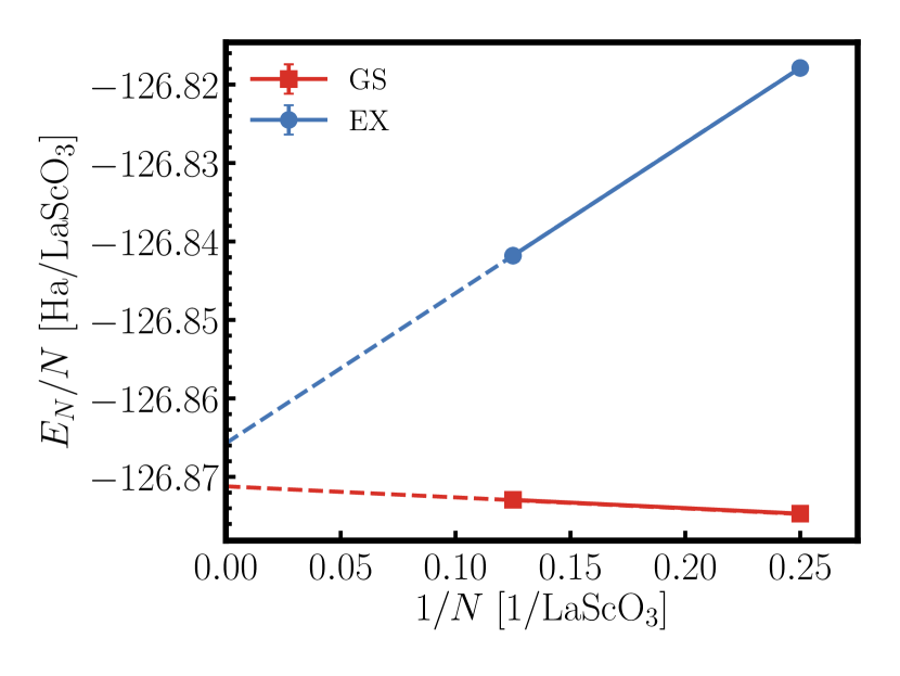
(a)

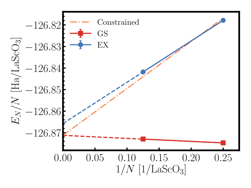
(b)

Figure 4: a) Extrapolations of ground (squares) and excited (circles) state energies per unit using 20- and 40-atom supercells data. Note that the extrapolated energies do not agree by a significant margin since the corresponding error bars are about 1 mHa/unit (ie, smaller than the data symbols). b) We add the constrained extrapolation of the excited state with the asymptotic value identical to the ground state. As explained in the text, any asymptotic value within a reasonable energy range (eg, plotted vertical axis range) that is applied consistently to both state extrapolations leads to the same gap value.

Let us now outline how we address these complications and also propose an approach on how to extract the gap from our data set.

i) Total energy offsets. We first address the asymptotic energy offsets, ie, $A$ and $A^{ex}$, by considering that they do not necessarily have the same value. Although the offsets should nominally vanish for $N\to\infty$, it is well-known that the conditionally convergent Ewald sums can exhibit finite, ${\cal O}(1)$ terms, in the thermodynamic limit (e.g., from nonvanishing multipole moment densities, such as quadrupole moments). Similarly, the kinetic energy could converge slowly for metals Drummond et al. (2008) or in the vicinity of critical points in electronic phase diagrams, etc. Related effects were addressed by corrections using real or reciprocal space formulations Hunt et al. (2018); Yang et al. (2019); Chiesa et al. (2006); McClain et al. (2017). Furthermore, any contribution of sub-leading terms would effectively add to $A,A^{ex}$ within our range of sizes as mentioned aboveMcClain et al. (2017). The key observation for our data is that the ground state value of $A$ appears to be rather small, see Table 7 and Fig. 4(a). We assume that this reflects a gradual convergence due to appreciably large number of electrons/states already in the primitive cell and rather flat bands in comparison with the expected size of the band gap. On the other hand, the excited state slope is an order of magnitude larger than for the ground state. Therefore we expect that $A^{ex}$ contained in the excited state slope has a similar value so that it does not overshadow the gap “signal”. Assuming that $A\approx A^{exc}$ is approximately true, we can cancel out most of this bias using the difference $A-A^{ex}$. We then expect that the remaining error would then be only a fraction of the ground state slope or perhaps even smaller. The impact of such residual error on the gap estimation would then be below our statistical uncertainty. Note that we have seen similar behavior in a previous study of phosphorene that showed essentially converged ground state thus enabling accurate gap estimation Frank et al. (2019).

We note that this assumption might not always be valid. A possible situation where such assumption could fail can occur if the ground state slope happens to be large and comparable to the excited state slope. Such complication can make the gap estimation difficult or biased. Obviously, this would require further data for larger sizes and/or detailed analysis of the sources of biases involved.

ii) Cohesion differences. Biases in the asymptotic values $e_{0},e_{0}^{ex}$ could influence the results even more significantly. Although these values should nominally agree, in many calculations they still differ by a statistically significant margin suggesting an apparent thermodynamic limit inconsistency. For our case, see Table 7 and Fig. 4(a), the corresponding limits differ by at least six standard deviations. Regardless what is the source of the disagreement, if that would persist even for larger supercells the resulting biases would be difficult to control. It is then inevitable that the band gap estimations from raw differences of total energies lead to a bias and that, contrary to the intuition, its influence on total energy differences can even grow with the supercell size. Although our data indicates a seemingly “small” difference (i.e., well below 1 mHa/unit for 40 atom system), for the total energies it is indeed very significant. We address this problem by an approximate cohesion consistency condition that requires both extrapolations to converge to the same asymptotic value, which we label as $e_{0}^{asym}$. This effectively restricts $e_{0}=e_{0}^{exc}=e_{0}^{asym}$ and forces both extrapolations to be consistent in the thermodynamic limit. The corrected value of the gap is then estimated from the difference of the corresponding slopes. For simplicity, let us first assume that $e_{0}^{asym}$ is bounded by the given data range

$$e_{0}\leq e_{0}^{asym}\leq e_{0}^{ex}.$$ (7)

In Fig. 4(b), we use the ground state value of $e_{0}$ (that is intuitively perhaps the most appropriate choice) as the common asymptotic limit. Interestingly, the condition above can be relaxed and the true asymptotic value could possibly be outside this bound (note that the considered data is based on single $k-$point occupation). The construction is very robust in this sense since the corresponding gap estimation does not depend on the precise value of $e_{0}^{asym}$. Indeed, any value from a reasonable energy range gives the same gap (basically, due to the conserved sum of angles in a triangle so that the difference between the slopes does not change). From this analysis we therefore conclude that the lack of consistency of energy/unit asymptotic values does play a significant role in biasing the total energy differences. Considering broader implications, if the difference between these asymptotic values is unacceptably large it simply indicates that calculations of larger supercells are still necessary in order to obtain a reliable result. In our experience so far, if the ground state varies mildly with the cell size, restoring the convergence of both extrapolations to the same asymptotic cohesion removes most or at least a major part of the finite size bias. (We have additional example(s) where essentially perfect agreement in extrapolated cohesions is achieved directly from the data and indeed the gap estimation is then more straightforward, to be published elsewhere.)

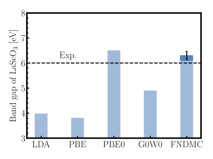
Figure 5: Band gaps of LaScO₃ from LDARavindran et al. (2004), PBEHe and Franchini (2012), PBE0 (this work), $G_{0}W_{0}$ Ergönenc et al. (2018), and FNDMC (this work) compared with the experimental estimation. FNDMC is given as 6.30(17) eV, whereas the estimated of $\approx$ 0.2 eV fixed-node bias is indicated by the shaded region.

Our consistency construction leads to the gap estimation of 6.30(17) eV. In order to complete the considerations of systematic biases, we conjecture that the fixed-node bias is between $0.1-0.2$ eV, based on experience from previous calculations Kolorenč et al. (2010). Taking this into account, the resulting best guess with all (known) systematic and random errors leads to estimate of 6.10 - 6.20 (17) eV, that is indeed very close to the experiments. We recall that the optical experimental data show onset of absorption at $\approx 6$ eV at ambient temperatures. For $T=0$ though, removing the zero point and thermal motion effects of would increase the measured gap at least by $0.1$ eV if not more, considering corrections from electron-phonon effects in large gap solids with similar elements Cannuccia and Marini (2011); Bhandari et al. (2018). In fact, the resulting agreement we see is perhaps beyond expectations from a single-reference trial wave function DMC method and corroborates the previous findings that have produced accurate values for cohesive and low-lying excitations of solids. A comparison of gap estimations to experiment for various electronic structure methods is shown in Fig. 5.

The presented construction is approximate and clearly has certain applicability limits. In particular, the data should be close to the thermodynamic limit with the ground state close to being converged in the first place. If this is not the case and the slopes for the ground and excited states are very similar and possibly large, the “gap signal” might be simply lost in the statistical noise and/or present systematic biases. Biases could be caused if the offsets vary from size to size due to non-cubic cell shapes or very different aspect ratios. Although the aspect ratio changes in our case of a 20 vs. 40 atom supercell, we rely on the key feature of our band structure with a large gap and relatively flat bands. However, in general further complications could stem from slow convergence of energy components or other features such as charges, defects, etc. and may prevent reliable estimations. Further issues could emerge for systems with very small gaps and/or metals. Therefore, for such applications further study of finite size effects at realistic supercells sizes is highly desirable.

Table 7: FNDMC total energies [Ha] calculations of the various states used to estimate the gaps from raw energy differences $\Delta_{\rm op},\Delta_{\rm qp}$ [eV]. We perform each calculation for the supercell $\Gamma$ point, which allows us to directly target the CBM and VBM in each supercell. There is essentially perfect agreement between optical and fundamental gaps that suggest no presence of excitonic signals. We provide the total energies and calculate the gaps from the direct energy differences, that are not corrected for finite size effects.

State/Cell	20 atom	40 atom
$E_{N}(\Gamma)$	-507.4987(22)	-1014.9833(28)
$E_{N+1}(\Gamma)$	-506.9369(40)	-1014.4147(09)
$E_{N-1}(\Gamma)$	-507.8305(50)	-1015.3112(19)
$E_{N}^{exc}(\Gamma$)	-507.2715(15)	-1014.7344(22)
$\Delta_{\rm qp}$ (eV)	6.26(20)	6.79(32)
$\Delta_{\rm op}$ (eV)	6.18(08)	6.89(23)

Table 8: FNDMC energies [Ha] per LaScO₃ for ground and excited states used to eliminate the finite size effects from the estimation of the optical gap [eV] from differences ($\Delta$) as well from the slopes ($E_{g}$ ) with finite size correction.

State/Cell	20 atoms	40 atoms	$e_{0}$ + const$/N$
$E_{N}(\Gamma)/N$	-126.87468(55)	-126.87292(36)	-126.8712(12) $-0.0141(51)/N$
$E_{N}^{exc}(\Gamma)/N$	-126.81788(38)	-126.84180(28)	-126.86572(74) +0.1914(37)/$N$
$E_{N}^{exc}(\Gamma)/N$	-126.81788(38)	-126.84180(28)	-126.8712(12) $+0.2175(37)/N$
$e_{0}^{exc}\leftarrow e_{0}$
Gap			$E_{g}$ (finite size corrected)
$\Delta_{\rm op}$ (eV)	6.18(08)	6.89(23)	6.30(17)

Discussion. We initiate the discussion by recalling some of the previously published results. As it is well-known DFT methods have their limitations and in particular the description of excitations can lead to rather mixed results. One of the reasons is the tendency to smooth out and distort the excited states by systematic deficiencies in approximate functionals (such as the lack of self-interaction correction) that typically leads to underestimated band gaps. Extensions to DFT such as hybrid functionals, through inclusion of some of the exact exchange, correct for part of these errors and often result in rather close agreement with experiments even with little fine-tuning. Hybrid functionals are often reasonable using their default values of exact exchange mixing, and previous calculations with HSE find a bandgap of 5.73 eV He and Franchini (2012), whereas our independent calculations with PBE0 find a bandgap of roughly 6.51 eV using the default parameters. While these estimates are not perfect, they are relatively close to the experimental values. Improvements for hybrids can be obtained by retuning the exact exchange parameter, however this requires one to have experimental data to compare against and is not purely ab initio. Many-body perturbation theory such as $G_{0}W_{0}$ is often used to improve the DFT band gap issues. However, the results can be rather sensitive to the underlying DFT orbitals Zhao and Neuscamman (2019). A very systematic study using $G_{0}W_{0}$ was carried out for a wide variety of ABO₃ compounds, and for the majority the calculated band gaps largely agree with experiment. However for LaScO₃ the $G_{0}W_{0}$ bandgap is estimated to be between 4.5 and 4.9 eV Ergönenc et al. (2018). This discrepancy with experiments is justified by stating: “LaScO₃ is a clear band insulator with the first (charge-transfer) optical excitation arising from the O$-p$ to Sc$-d$ transition; the experimental spectrum does not clearly show the tail at the bottom of the spectrum well visible in $GW$. We believe that the $GW$ band structure is reliable in this respect, and that the onset of optical absorption is not easily detected in the experiment. We therefore trust that our predicted band gap of 4.9 eV should be more reliable than the experimental estimate of 6.0 eV.” We would like make the following comments on two aspects of this interesting material. One point to consider is that the $3d$-channel is not the only candidate for the lowest excitations stemming mainly from the Sc atom. The actual situation might be more complex and probably involves a number of channels and many-body effects. In this respect, there is a rather unique example of bounded atomic Sc^- anion for which one expects the ground state to be a triplet with additional electron occupying the $d$-orbital, ie, ${}^{3}F(3d^{2}4s^{2})$. Surprisingly, this is incorrect and such a state is not bounded Mitáš (1993); Hotop and Lineberger (1985). The true Sc^- bounded lowest state actually does not conform to the Hund’s rules; it is a singlet and the additional electron goes to the $4p$ state, i.e., it is ${}^{1}D(3d4s^{2}4p)$, showing nontrivial correlations and competition of several one-particle atomic channels. We believe that such correlations might be quite difficult to describe even by sophisticated and precise perturbational approaches and indeed many-body wave functions are crucial for describing such effects Mitáš (1993).

Furthermore, we also consider the fact that absorption data could be challenging to analyze when the band gap is large. However, the underestimation from $GW$ using PBE orbitals does not necessarily imply the stated claim, given the significant variability of typical $GW$ results with respect to their underlying orbital sets Zhao and Neuscamman (2019). Our DMC results indicate that the gap, at least in the ideal system without defects or non-stoichiometries, appears to be around or marginally above $\approx$ 6 eV, in an excellent agreement with several published spectra. Therefore we are inclined to accept the optical experiments as representative in this regard. High quality direct and inverse photoemission experiments for LaScO₃ would be highly desirable in corroborating the results of both our calculations as well as the data from existing optical measurements.

IV Conclusions

We present a quantum Monte Carlo study of LaScO₃ based on real space sampling and fixed-node diffusion Monte Carlo method. Experiments show that this scandate is a large gap nonmagnetic insulator as has been consistently reconfirmed by several experiments. Despite the fact that optical data is often more complex to analyze, for large dielectric materials the lowest excitations should effectively measure the fundamental gap due to absence of strong excitons. In this Mott-Wannier limit, the interaction between electrons and holes is largely screened, and the resulting excitons are delocalized with a very small binding energy.

Our calculations are based on standard the DMC workflow and we are able to obtain accurate band gaps when compared to experiment, without the need for fine-tuning any non-variational parameters. Other electronic structure methods rely on guidance from experiments, such as adjusting the exact exchange mixing parameter in hybrid functionals or inserting Hubbard $U$ in DFT+$U$ approaches. Similarly, changing the initial orbitals sets, i.e., the starting point bias in $GW$ methods can affect and possibly bias the predictions as well. As an alternative, diffusion Monte Carlo relies only on the variational principle and on the quality of the nodal set of the explicitly constructed many-body trial wave function. Note that the usual issue of finite basis set in correlated wave function methods does not arise in DMC since the random walks represent sampling of the complete position space. We show that for systems such ours, the standard ansatz for excited states such as promotion from the valence to the conduction band works quite well when coupled with the nodal surface optimization using one-parameter hybrid DFT effective Hamiltonian.

We have carried out also a rather detailed study of finite size effects such as twist averages for the proper estimation of cohesion. In fact, our cohesive energy is a genuine prediction since to the best of our knowledge that quantity has not been measured yet. Similarly, we have studied the finite size biases in estimations of the band gap for different supercell sizes. Since our system exhibits relatively flat bands when compared with the gap, we have encountered rather mild finite size dependence of the ground state at intermediate sizes. We then showed that it is important to take into consideration both the ground and excited states scaling to large sizes so as to guarantee the consistency in thermodynamic limit. Using this as a consistency condition has enabled us to conclude that the band gap is located at 6 eV and possibly marginally higher. Based of previous transition metal oxide QMC calculations we conjecture that the bias from the fixed-node approximation is around 0.1 to 0.2 eV which is essentially on par with our statistical resolution.

Although our agreement with the experiment is very encouraging we would like to reflect on the origin of systematic errors still involved. We recapitulate the following possible sources:

a) Finite size effects, which we treat approximately, are still very important for further considerations. This concerns both the offsets and sub-leading order terms that could be still significant at intermediate sizes. Within the presented data the gap estimation is essentially locked by the introduced consistency condition at the asymptotic limit, however, for other quantities more studies and insights are necessary.

b) Residual fixed-node errors that remain after taking differences are equally relevant. The goal is to get the resulting fixed-node bias to such level that it would not affect the differences of interest within the desired statistical accuracy. Obviously, for larger systems the cost and difficulty of such exploration can be very very challenging.

c) Neglect of zero point and thermal motion effects on the band gap and possibly other quantities of interest. For these effects we roughly estimate that their impact on the band gap is of the order of 0.1 eV. Here we consider some of the recent results Bhandari et al. (2018); Nery et al. (2018) for transition and simple metal oxide materials such as SrTiO₃, TiO₂ and SnO₂ where phononic corrections are in the range $\approx$ 0.1 and 0.3 eV. This clearly requires further study.

In order to cross-validate a number of technical aspects of the QMC methodology, most of the calculations have been carried out along two independent tracks. One used the Qwalk code with gaussian basis sets, correlation consistent ECPs (ccECPs), and the Crystal code for generating the self-consistent gaussian-based solid state orbitals. The other track employed DFT-generated pseudopotentials, Quantum Espresso code with plane wave basis and Qmcpack for QMC runs. Overall, we find excellent agreement between the results using these technically very different paths, independent codes, effective Hamiltonians and basis sets. These two sets of results provide a systematic corroboration of the robustness of the QMC methods and tools for calculations of transition metal oxide systems and other complex materials in future.

For more complicated systems and further gains in accuracy, systematic improvement of the ground and excited states may be necessary Zhao and Neuscamman (2019). In addition, better understanding of finite size effects for realistic sizes of supercells will be also an important subject of future studies. Nevertheless, the methods presented here provide an excellent starting point and a first step towards more accurate and further elaborated ab inito calculations where more sophisticated trial wave function ansatz may be necessary, beyond just the Slater-Jastrow form.

Acknowledgements

This work presents two sets of quantum Monte Carlo results, methodologies, packages and calculations. The work based on the QMCPACK package and associated tools ($\approx 50$% of the project) has been supported by the U.S. Department of Energy, Office of Science, Basic Energy Sciences, Materials Sciences and Engineering Division, as part of the Computational Materials Sciences Program and Center for Predictive Simulation of Functional Materials.

The authors would like to thank Luke Shulenburger for reading the manuscript and for comments.

The presented work that used the QWalk package and corresponding tools ($\approx 50$% of the project) has been supported by the U.S. Department of Energy, Office of Science, Basic Energy Sciences (BES) under the award de-sc0012314.

The calculations were performed at Sandia National Laboratories and at TACC under XSEDE.

Sandia National Laboratories is a multi-mission laboratory managed and operated by National Technology and Engineering Solutions of Sandia LLC, a wholly owned subsidiary of Honeywell International, Inc. for the U.S. Department of Energy’s National Nuclear Security Administration under Contract No. DE-NA0003525.

This paper describes objective technical results and analysis. Any subjective views or opinions that might be expressed in the paper do not necessarily represent the views of the U.S. Department of Energy or the United States Government.

References

- Pari et al. (1995) G. Pari, S. Mathi Jaya, G. Subramoniam, and R. Asokamani, Phys. Rev. B 51, 16575 (1995).
- He and Franchini (2012) J. He and C. Franchini, Phys. Rev. B 86, 235117 (2012).
- Ergönenc et al. (2018) Z. Ergönenc, B. Kim, P. Liu, G. Kresse, and C. Franchini, Phys. Rev. Materials 2, 024601 (2018).
- Santana et al. (2017) J. A. Santana, J. T. Krogel, P. R. C. Kent, and F. A. Reboredo, The Journal of Chemical Physics 147, 034701 (2017), https://doi.org/10.1063/1.4994083 .
- Afanas’ev et al. (2004) V. V. Afanas’ev, A. Stesmans, C. Zhao, M. Caymax, T. Heeg, J. Schubert, Y. Jia, D. G. Schlom, and G. Lucovsky, Applied Physics Letters 85, 5917 (2004), https://doi.org/10.1063/1.1829781 .
- Arima et al. (1993) T. Arima, Y. Tokura, and J. B. Torrance, Phys. Rev. B 48, 17006 (1993).
- Heeg et al. (2006) T. Heeg, J. Schubert, C. Buchal, E. Cicerrella, J. Freeouf, W. Tian, Y. Jia, and D. Schlom, Applied Physics A 83, 103 (2006).
- Dang et al. (2014) H. T. Dang, X. Ai, A. J. Millis, and C. A. Marianetti, Phys. Rev. B 90, 125114 (2014).
- Geller (1957) S. Geller, Acta Crystallographica 10, 243 (1957).
- Clark et al. (1978) J. Clark, P. Richter, and L. D. Toit, Journal of Solid State Chemistry 23, 129 (1978).
- Momma and Izumi (2011) K. Momma and F. Izumi, Journal of Applied Crystallography 44, 1272 (2011).
- Foulkes et al. (2001) W. M. C. Foulkes, L. Mitas, R. J. Needs, and G. Rajagopal, Rev. Mod. Phys. 73, 33 (2001).
- Melton and Mitas (2017) C. A. Melton and L. Mitas, Phys. Rev. E 96, 043305 (2017).
- Umrigar et al. (2007) C. J. Umrigar, J. Toulouse, C. Filippi, S. Sorella, and R. G. Hennig, Phys. Rev. Lett. 98, 110201 (2007).
- Hunt et al. (2018) R. J. Hunt, M. Szyniszewski, G. I. Prayogo, R. Maezono, and N. D. Drummond, Phys. Rev. B 98, 075122 (2018).
- Yang et al. (2019) Y. Yang, V. Gorelov, C. Pierleoni, D. M. Ceperley, and M. Holzmann, “Electronic band gaps from quantum monte carlo methods,” (2019), arXiv:1910.07531 [cond-mat.mtrl-sci] .
- Frank et al. (2019) T. Frank, R. Derian, K. Tokar, L. Mitas, J. Fabian, and I. Stich, Physical Review X 9, 011018 (2019).
- Foulkes et al. (1999) W. M. C. Foulkes, R. Q. Hood, and R. J. Needs, Phys. Rev. B 60, 4558 (1999).
- Zhao and Neuscamman (2019) L. Zhao and E. Neuscamman, Phys. Rev. Lett. 123, 036402 (2019).
- Heeg et al. (2005) T. Heeg, M. Wagner, J. Schubert, C. Buchal, M. Boese, M. Luysberg, E. Cicerrella, and J. Freeouf, Microelectronic Engineering 80, 150 (2005), 14th biennial Conference on Insulating Films on Semiconductors.
- Wagner et al. (2009) L. K. Wagner, M. Bajdich, and L. Mitas, Journal of Computational Physics 228, 3390 (2009).
- Kim et al. (2018) J. Kim, A. D. Baczewski, T. D. Beaudet, A. Benali, M. C. Bennett, M. A. Berrill, N. S. Blunt, E. J. L. Borda, M. Casula, D. M. Ceperley, S. Chiesa, B. K. Clark, R. C. Clay, K. T. Delaney, M. Dewing, K. P. Esler, H. Hao, O. Heinonen, P. R. C. Kent, J. T. Krogel, I. Kylänpää, Y. W. Li, M. G. Lopez, Y. Luo, F. D. Malone, R. M. Martin, A. Mathuriya, J. McMinis, C. A. Melton, L. Mitas, M. A. Morales, E. Neuscamman, W. D. Parker, S. D. P. Flores, N. A. Romero, B. M. Rubenstein, J. A. R. Shea, H. Shin, L. Shulenburger, A. F. Tillack, J. P. Townsend, N. M. Tubman, B. V. D. Goetz, J. E. Vincent, D. C. Yang, Y. Yang, S. Zhang, and L. Zhao, Journal of Physics: Condensed Matter 30, 195901 (2018).
- Dovesi et al. (2005) R. Dovesi, A. Erba, B. Civalleri, C. Roetti, V. Saunders, and C. Zicovich-Wilson, Zeitschrift für Kristallographie - Crystalline Materials 220, 571 (2005).
- Dovesi et al. (2009) R. Dovesi, V. Saunders, C. Roetti, R. Orlando, C. Zicovich-Wilson, F. Pascale, K. Doll, N. Harrison, I. Bush, P. D’Arco, and M. Llunell, CRYSTAL09 User’s Manual. University of Torino, Torino (2009).
- Annaberdiyev et al. (2018) A. Annaberdiyev, G. Wang, C. A. Melton, M. Chandler Bennett, L. Shulenburger, and L. Mitas, The Journal of Chemical Physics 149, 134108 (2018), https://doi.org/10.1063/1.5040472 .
- Bennett et al. (2017) M. C. Bennett, C. A. Melton, A. Annaberdiyev, G. Wang, L. Shulenburger, and L. Mitas, The Journal of Chemical Physics 147, 224106 (2017), https://doi.org/10.1063/1.4995643 .
- Dolg et al. (1989) M. Dolg, H. Stoll, A. Savin, and H. Preuss, Theoretica chimica acta 75, 173 (1989).
- Dolg et al. (1993) M. Dolg, H. Stoll, and H. Preuss, Theoretica chimica acta 85, 441 (1993).
- Giannozzi et al. (2009) P. Giannozzi, S. Baroni, N. Bonini, M. Calandra, R. Car, C. Cavazzoni, D. Ceresoli, G. L. Chiarotti, M. Cococcioni, I. Dabo, A. Dal Corso, S. de Gironcoli, S. Fabris, G. Fratesi, R. Gebauer, U. Gerstmann, C. Gougoussis, A. Kokalj, M. Lazzeri, L. Martin-Samos, N. Marzari, F. Mauri, R. Mazzarello, S. Paolini, A. Pasquarello, L. Paulatto, C. Sbraccia, S. Scandolo, G. Sclauzero, A. P. Seitsonen, A. Smogunov, P. Umari, and R. M. Wentzcovitch, Journal of Physics: Condensed Matter 21, 395502 (19pp) (2009).
- Giannozzi et al. (2017) P. Giannozzi, O. Andreussi, T. Brumme, O. Bunau, M. B. Nardelli, M. Calandra, R. Car, C. Cavazzoni, D. Ceresoli, M. Cococcioni, N. Colonna, I. Carnimeo, A. D. Corso, S. de Gironcoli, P. Delugas, R. A. D. Jr, A. Ferretti, A. Floris, G. Fratesi, G. Fugallo, R. Gebauer, U. Gerstmann, F. Giustino, T. Gorni, J. Jia, M. Kawamura, H.-Y. Ko, A. Kokalj, E. Küçükbenli, M. Lazzeri, M. Marsili, N. Marzari, F. Mauri, N. L. Nguyen, H.-V. Nguyen, A. O. de-la Roza, L. Paulatto, S. Poncé, D. Rocca, R. Sabatini, B. Santra, M. Schlipf, A. P. Seitsonen, A. Smogunov, I. Timrov, T. Thonhauser, P. Umari, N. Vast, X. Wu, and S. Baroni, Journal of Physics: Condensed Matter 29, 465901 (2017).
- Kleinman and Bylander (1982) L. Kleinman and D. M. Bylander, Phys. Rev. Lett. 48, 1425 (1982).
- Drummond et al. (2016) N. D. Drummond, J. R. Trail, and R. J. Needs, Phys. Rev. B 94, 165170 (2016).
- Rappe et al. (1990) A. M. Rappe, K. M. Rabe, E. Kaxiras, and J. D. Joannopoulos, Phys. Rev. B 41, 1227 (1990).
- Krogel et al. (2016) J. T. Krogel, J. A. Santana, and F. A. Reboredo, Phys. Rev. B 93, 075143 (2016).
- Wagner and Mitas (2003) L. Wagner and L. Mitas, Chemical Physics Letters 370, 412 (2003).
- Kolorenč et al. (2010) J. Kolorenč, S. Hu, and L. Mitas, Phys. Rev. B 82, 115108 (2010).
- Ramer and Rappe (1999) N. J. Ramer and A. M. Rappe, Phys. Rev. B 59, 12471 (1999).
- Ravindran et al. (2004) P. Ravindran, R. Vidya, H. Fjellvag, and A. Kjekshus, Journal of Crystal Growth 268, 554 (2004), iCMAT 2003, Symposium H, Compound Semiconductors in Electronic and Optoelectronic Applications.
- McClain et al. (2017) J. McClain, Q. Sun, G. K.-L. Chan, and T. Berkelbach, J. Chem. Theory Comput. 13, 1209 (2017).
- Drummond et al. (2008) N. D. Drummond, R. J. Needs, A. Sorouri, and W. M. C. Foulkes, Phys. Rev. B 78, 125106 (2008).
- Chiesa et al. (2006) S. Chiesa, D. M. Ceperley, R. M. Martin, and M. Holzmann, Phys. Rev. Lett. 97, 076404 (2006).
- Cannuccia and Marini (2011) E. Cannuccia and A. Marini, Phys. Rev. Lett. 107, 255501 (2011).
- Bhandari et al. (2018) C. Bhandari, M. van Schilfgaarde, T. Kotani, and W. R. L. Lambrecht, Phys. Rev. Materials 2, 013807 (2018).
- Mitáš (1993) L. Mitáš, in Computer Simulation Studies in Condensed-Matter Physics V, edited by D. P. Landau, K. K. Mon, and H.-B. Schüttler (Springer Berlin Heidelberg, Berlin, Heidelberg, 1993) pp. 94–105.
- Hotop and Lineberger (1985) H. Hotop and W. Lineberger, J. Phys. Chem. Ref. Data 14, 731 (1985).
- Nery et al. (2018) J. P. Nery, P. B. Allen, G. Antonius, L. Reining, A. Miglio, and X. Gonze, Phys. Rev. B 97, 115145 (2018).