Quantum criticality of the Rabi-Stark model at finite frequency ratios

Abstract

In this paper, we analyze the quantum criticality of the Rabi-Stark model at finite ratios of the qubit and cavity frequencies in terms of the energy gap, the order parameter, as well as the fidelity, if the Stark coupling strength is the same as the cavity frequency. The critical exponents are derived analytically. The energy gap and the length critical exponents are different from those in the quantum Rabi model and the Dicke model. The finite size scaling analysis for the order parameter and the fidelity susceptibility is also performed. The universal scaling behaviors are demonstrated and several finite size exponents can be then extracted. Furthermore, universal critical behavior can be also established in terms of the bosonic Hilbert space truncation number, and the corresponding critical scaling exponents are found. Interestingly, the critical correlation length exponents in terms of the photonic truncation number as well as the equivalently effective length scales are different in the Rabi-Stark model and the quantum Rabi model, suggesting they belong to different universality classes. The second-order quantum phase transition is convincingly corroborated in the Rabi-Stark model at finite frequency ratios, by contrast, it only emerges at the infinite frequency ratio in the original quantum Rabi model without the Stark coupling.

I Introduction

As advocated by Anderson that more is different  anderson , emergent phenomena occur when systems with many particles behave differently than their original few ones. In classical systems the transition between different phases is driven by thermal fluctuations. Similarly, quantum fluctuations can lead to transitions between distinct quantum phases of matter, such as superconductors and insulators  Sachdev . Recently, the quantum Rabi model (QRM) Rabi and Jaynes-Cummings model JC , both only describe a single-mode cavity field and a two-level atom, but interestingly exhibit the continuous quantum phase transition (QPT) plenio2015 ; plenio2016 ; MXLiu , thus extending the previous concept to systems with few degrees of freedom. To see the collective behaviors, one need enhance the atom-field interaction and increase the two level energy difference at the same time. The former requirement can be gradually satisfied with the recent progress on cavity quantum electrodynamics (QED)  CQED , circuit QED  Niemczyk ; Yoshihara ; Forn2 , and trapped ions Leibfried , which can realizes the QRM from strong coupling Clarke , ultra-strong coupling  Forn , and even to deep-strong coupling  Casanova .

The light-matter interaction can be engineered in many different ways. Benefiting from development of quantum simulation technology, the so-called quantum Rabi-Stark model (RSM) has been realized by adding an nonlinear process to the QRM Grimsmo1 ; Grimsmo2 , and the Hamiltonian is given by

$$H_{R}=\left(\frac{\Delta}{2}+Ua^{\dagger}a\right)\sigma_{z}+\omega a^{\dagger}a+g(a^{\dagger}+a)\sigma_{x},$$ (1)

where $\Delta$ and $\omega$ are frequencies of two-level system and cavity, $\sigma_{i}(i=x,y,z)$ are usual Pauli matrices describing the two-level system, $a$ ($a^{\dagger}$) are the annihilation (creation) bosonic operators of the cavity mode with frequency $\omega$, and $g$ denotes the linear coupling strength between the qubit and the cavity. The nonlinear coupling strength $U$ is determined by the dispersive energy shift. To me more concise, the units are taken of $\omega=1$ throughout this paper unless specified. It has been studied by the Bargmann approach Maciejewski ; Eckle and the more physical Bogoliubov operator approach  Xie2019 . It is found that the emergent Stark-like nonlinear interaction bring about the novel and exotic physical properties. Such as, the interaction induced energy spectra collapse can be observed in the limit of $U\rightarrow\pm 1$  Xie2019 above a critical atom-cavity coupling strength. The first-order QPT, indicated by the level crossing of the ground-state and first excited state, is also observed Xie2019 . Grimsmo and Parkins conjectured that the nonlinear dispersive-type coupling would possibly induce a new superradiant phase at this single atom level if  $U<-1$  Grimsmo1 in the open systems.

The RSM has been attracted much attention more recently. The implementation of the RSM was proposed using trapped ions Cong . In this proposal, external laser beams are applied to induce an interaction between an electronic transition and the motional degree of freedom, thus the Stark term is generated. A continuous quantum phase transition in the limit of $U\rightarrow\pm 1$ is suggested in terms of the energy gap closing at a critical coupling in the anisotropic RSM  Xie2020 .

In this paper, we study the quantum criticality around the critical coupling of the isotropic RSM in the limit of $U\rightarrow\pm 1$ at finite frequency ratio $\Delta/\omega$. The paper is structured as follows: In Sec. II, we proposed the evidence of the second-order QPTs in the RSM at finite frequency ratio by calculating the critical (dynamic) exponent of energy gap analytically and analyze the singularity of ground state energy numerically at $U=\pm 1$. We discuss the critical behavior of order parameter and its finite size scaling behavior in Sec. III. In Sec. IV, we propose the accurate hypothesis of fidelity susceptibility, and the nice scaling behavior is also observed. We further explore the effects of the truncation of the bosonic Hilbert space on the criticality in Sec. V, where the comparison to the criticality of the QRM is also given. Finally we give a summary and outlooks in Sec. VI. Appendix A provides the analytical derivation of some critical exponents and Appendix B shows both finite-size and finite-truncation analyses for the energy gap and the variance of position quadrature of the field.

II Critical behavior in terms of the energy gap and the ground-state energy

As found by Xie  et al.  Xie2019 , the RSM at $U=1$ can be mapped to an effective quantum harmonic oscillator. Thus the low energy spectra of Hamiltonian (1) can be easily given by

$$\frac{\sqrt{-\left(\frac{\Delta}{2}+E\right)}\left(E+1-\frac{\Delta}{2}\right)}{\sqrt{-\left(\frac{\Delta}{2}+E+2g^{2}\right)}}=2n+1,\quad n=0,1,2,...\infty.$$ (2)

where an infinite number of discrete energy levels is confined in the energy interval

$$\frac{\Delta}{2}-1<E<E_{c}^{+},$$ (3)

if $g<g_{c}^{+}$, where $\ g_{c}^{+}=\sqrt{(1-\Delta)/2}$ and $E_{c}^{+}=-\Delta/2-2g^{2}$. All discrete low energy levels collapse to $E_{c}^{+}$ at $g=g_{c}^{+}$, thus the energy gap closes at $\ g_{c}^{+}$, implying the occurrence of a second-order QPT in this model. For the case of $U=-1$, the extension can be achieved straightforwardly by changing $\Delta$ into $-\Delta$. As the implementation of the RSM in trapped ions proposed in Ref.  Cong , the Hamiltonian is derived in a rotated frame so that the shifting detuning $\Delta$  can be negative.

For $g>g_{c}^{+}$, it is observed from numerical exact diagonalizations that all energies become closer to $E_{c}^{+}$ monotonously with the increasing truncated Fock space, although the convergence is hardly achieved by numerics. We argue that the energy would be only $E_{c}^{+}=-\Delta/2-2g^{2}$, and resulting effective harmonic potential, $\omega_{eff}=\sqrt{1+2g^{2}/\left(\frac{\Delta}{2}+E\right)}$, is flat. Note that the energy could be any value for the flat potential. But the perquisite condition for flat potential is no other than $E=E_{c}^{+}$. It is therefore suggested that the gapless Goldstone mode excitations appear for $g>g_{c}^{+}$.

Below the critical points in the RSM, one can find that the ground-state has a conserved parity symmetry, odd parity for $U=1$, and even parity for $U=-1$  Xie2020 . Above the critical points, the parity symmetry is broken due to the infinite degeneracy for all states.

The analytical mean photon number $\overline{n}=\left\langle a^{\dagger}a\right\rangle$ in the ground-state is also found to diverge at $g_{c}^{+}$  Xie2019 . Infinite photons are activated at the critical coupling, signifying the emergence of a new quantum phase.

To corroborate the second-order QPT in the RSM, we then discuss critical behavior of energy gap and singularity of the second derivative of the ground-state energy.

As sown in Ref. Xie2020 , the energy gap between the ground-state and the first excited state follow the universal scaling behavior in the continuous QPT Sachdev

$$\varepsilon(g\rightarrow g_{c})\sim\left|g-g_{c}\right|^{z\nu_{x}},$$ (4)

where $g_{c}$ is $g_{c}^{+}$ ($g_{c}^{-})$ for $U=1(-1)$, $\nu_{x}$ is the critical exponent and $z$ is dynamical exponent. $z\nu_{x}$ is found to be $2$ as long as the counterrotating wave terms are present.

As given analytically in detail in Eq. (22) of the Appendix A, the variance of position quadrature of the field diverge as $\Delta x=\sqrt{\left\langle x^{2}\right\rangle-\left\langle x\right\rangle^{2}}\propto(g_{c}^{+}-g)^{-\frac{1}{2}}$. It suggests $\nu_{x}=\frac{1}{2}$, and thus implies $z=4,$ in the RSM. In contrast, the gap exponent $z\nu_{x}=1/2$ with $\nu_{x}=1/4\$and $z=2\$has been found in both the Dicke model Emary and the QRM  plenio2015 . Therefore the RSM is not in the same universality class as the Dicke model and the QRM.

The phase transition takes places in the thermodynamic limit with the emergence of singularity of some physical observables. Despite few degrees of freedom in the QRM, the effective system size could be defined as $L_{R}=\Delta/\omega$ plenio2015 in order to catch sight of the critical behavior of the phase transitions. The singularity only appears in the limit of $\Delta/\omega\rightarrow\infty$. Since the energy gap closes only at $U=\pm 1$ in the present RSM, we may define the system size here as

$$L=\frac{1}{1\mp U}.$$ (5)

With this definition, $U=\pm 1$ is just corresponding to the thermodynamic limit.

As long as $\left|U\right|<1$, the ground-state energy at arbitrary coupling strength can be in principle calculated exactly. We then look at its derivatives at the critical points $g_{c}^{\pm}=\sqrt{(1\mp\Delta)/2}$ for finite effective sizes $L(U)$, and inspect how it evolves with the increase of the system size. The exact solution can be obtained by either the G-function approach  Xie2019 or the direct exact diagonalzations in truncated Fock space. Figure 1 presents the first-order (left panel) and the second-order  (right panel) derivatives of the ground state energy for $U$ gradually approaching to $\pm 1$, i.e. the size $L$ tends to infinity. One can find that the first-order derivative is always continuous when $U\rightarrow\pm 1$, while its second-order derivative changes drastically with system size $L$, displaying the discontinuity in the trend. It thus provides the another evidence of the second-order QPT in this model. It should be pointed out that it is extremely difficult to obtain the converged results in the both approaches if $U$ further approaches to $\pm 1$.

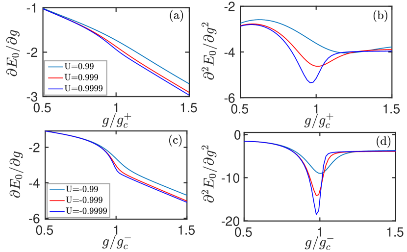
Figure 1: The first- and second-order derivative of the ground-state energy by the numerically exact solution of the RSM at $\Delta=0.5$ for different $U$ approaching to $1$ (upper panel) and $-1$ (lower panel).

We will perform the finite-size scaling analysis  on the order parameter and fidelity by using the above definition of the effective system size below.

III Order parameter and finite-size scaling analysis

To characterize the continuous QPT, we should define the order parameter. In QRM  plenio2015 , the re-scaled cavity photon number $\overline{n}=\left\langle a^{\dagger}a\right\rangle$ can be regarded as the order parameter since it is zero below and finite above the critical points.  But in the present RSM it is always finite below and diverges at the critical point.  We may define the inverse photon number $1/\overline{n}$ as the order parameter $M$. It is finite below $g_{c}^{+}$, and tends to zero at $g_{c}^{+}$. Eq.(34) in Ref. Xie2019 in the limit of $g\rightarrow g_{c}^{+}$ can be rewritten as

$$\overline{n}=\frac{6g^{2}\left(g_{c}^{+2}-g^{2}\right)}{E_{c}^{+}-E_{0}}+\frac{3}{16\left(g_{c}^{+2}-g^{2}\right)}\propto\left(g_{c}^{+}-g\right)^{-1},$$ (6)

Thus the exponent for order parameter is $\beta=1$. The detailed derivation of Eq. (6) is also given in Eq. (21) in Appendix A.

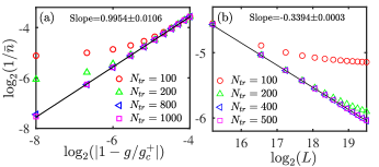
Figure 2: (a) The log-log plot of the order parameter $1/\overline{n}$ as a function of $\left|1-g/g_{c}^{+}\right|$ before $g_{c}$ for different truncation photon numbers $N_{tr}$. The fitting slope is very close to 1. $U=1$ and $\Delta=0.5$. (b) The log-log plot of order parameter $1/\overline{n}$ as a function of system size $L$ at $g_{c}$. The fitting slope is very close to $-1/3$. $\Delta=0.5$.

To confirm the analytical findings, we perform the numerically diagonalization of the RSM, which requires the truncation of the bosonic Hilbert space. Figure  2 (a) shows the order parameter $1/\overline{n}$ as a function of the reduced coupling constant $t=1-g/g_{c}^{+}$ on a log-log scale before $g_{c}^{+}$ by numerics for different truncation photon numbers $N_{tr}$. One can find that the convergence can be achieved for very large $N_{tr}$. A power law behavior, $1/\overline{n}\propto|1-g/g_{c}^{+}|^{\beta},$ is gradually exhibited in a wider the critical regime with increasing $N_{tr}$. The slope of the fitting line indicates that $\beta$ is just close to $1$. A log-log plot for the order parameter versus the system size for different truncation photon numbers at the critical point $g_{c}^{+}$ is also presented in Fig. 2 (b). Note that for finite size systems, i.e. $\ U$ is away from $1$, the convergence is arrived at more quickly with increasing $\ N_{tr}$, compared to the thermodynamic limit $\ U=1$.  A perfect power-law behavior, $1/\overline{n}\propto L^{-\gamma}$, is clearly shown for the large truncation $N_{tr}$. The fitted value of the scaling exponent $\gamma$ is very close to $1/3$. Through extensive calculations, one can find that both $\beta$ and $\gamma$ are independent of the values of $\Delta$.

The finite-size scaling for the order parameter can be also performed. In the critical regime of the continuous phase transition, it should satisfy the finite-scaling ansatz for the homogeneous function $M(\lambda^{h_{t}}t,\lambda^{h_{L}}L)=\lambda M(t,L)$, where $\lambda$ is the scale factor and $h_{t,L}$ related to some exponents below. Accordingly, the homogeneous function takes the following form

$${M}=|t|^{\beta}m(|t|L^{\gamma/\beta}),$$ (7)

where $\beta$ is the order parameter exponent and $\gamma$ is the finite-size scaling exponent for the order parameter. The function $m$ should be universal for large system size in the second-order QPT. $\nu=\gamma/\beta$ is the correlation length exponent due to the scaling function Eq. (7).

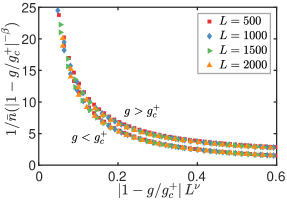
Figure 3: Finite size scaling for order parameter $1/\overline{n}$ according to Eq. (7) for both above and below the critical point at $U=1$ and $\Delta=0.5$.

By numerically diagonalizing the RSM, we show the finite-size scaling according to Eq. (7), where $M$ is just the order parameter $1/\overline{n}$, for different values of $L$ above and below the critical point in Fig. 3. A very large truncation number ($N_{tr}=1000$) for photon space is used to ensure that all numerical results in the finite size are converged. Here within the two exponents $\beta=1$ and $\gamma=1/3$ obtained above independently (cf. Fig. 2), an excellent collapse to the single curve in the critical regime is achieved for different large sizes. Two universal functions above and below the critical points are not required to be the same  plenio2015 . The universal scaling behavior observed here corroborates the continuous QPTs in the RSM at $U=1$. The correlation length exponent of the RSM is clearly $\nu=1/3$ in terms of the length definition (5).

IV FIDELITY SUSCEPTIBILITY and finite-size scaling analysis

The ground state fidelity can be taken as an useful tool to detect the QPTs even without the knowledge of the order parameters Gu2007 ; Gu2008 . It is defined as the overlap of the ground state wavefunctions at very close coupling parameters $g$ and $g+\delta g$ as

$$F(g,\delta g)=\left|\left\langle\psi_{0}(g)|\psi_{0}(g+\delta g)\right\rangle\right|.$$

The singularity of critical point would inevitably leads to the wavefunction experiencing dramatically change when crossing the critical point, showing a sharp change of fidelity.

Correspondingly, the fidelity susceptibility can be defined as Gu2007

$$\chi_{F}(g)=\lim_{\delta g\rightarrow 0}\frac{-2\ln F(g,\delta g)}{\delta g^{2}},$$

and can be written in terms of the eigenstates of the Hamiltonian

$$\chi_{F}(g)=\sum_{n\neq 0}\frac{\left|\left\langle\psi_{n}(g)\right|H_{I}\left|\psi_{0}(g)\right\rangle\right|^{2}}{\left[E_{n}(g)-E_{0}(g)\right]^{2}},$$ (8)

which is the leading order of the change in the fidelity.

In the critical regime, the fidelity susceptibility decays in a power law away from the critical point with critical exponent $\alpha$  Gu2008 ; Kwok2008

$$\chi_{F}\propto|g-g_{c}^{\pm}|^{-\alpha}.$$ (9)

In terms of the original definition of fidelity susceptibility Gu2010

$$\chi_{F}=\left<\frac{\partial\Psi_{0}}{\partial\lambda}\bigg{|}\frac{\partial\Psi_{0}}{\partial\lambda}\right>-\left<\frac{\partial\Psi_{0}}{\partial\lambda}\bigg{|}\Psi_{0}\right>\left<\Psi_{0}\bigg{|}\frac{\partial\Psi_{0}}{\partial\lambda}\right>,$$ (10)

we can actually derive the critical exponent of fidelity susceptibility $\alpha=2$ analytically, which is described in the end of Appendix A.

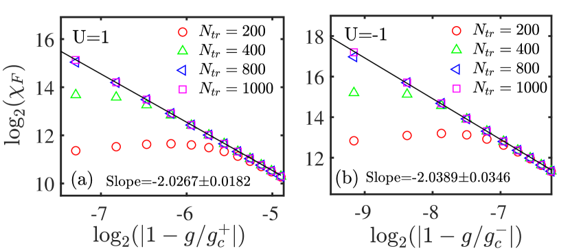
Figure 4: The log-log plot of fidelity susceptibility as a function of $g_{c}^{\pm}-g$ for different truncation photon numbers $N_{tr}$ at $U=1$ (left) and $-1$ (right). $\Delta=0.5$.

Similar to the order parameter, we present the fidelity susceptibility as a function of the deviation $g_{c}-g$ on a log-log scale below $g_{c}$ for $U=\pm 1$ by numerics within truncation of the bosonic Hilbert space in Fig. 4. Converged results are convincingly obtained with large truncation numbers. The converged data can be well fitted by straight lines with the same slope very close to $-2$, so we can immediately obtain its critical exponent $\alpha=2$, consistent with the analytical derivation.

In the second QPTs, the average fidelity susceptibility should follow the following finite-scaling ansatz Gu2007 ; Liu2009

$$\frac{\chi_{F}^{max}-\chi_{F}(g)}{\chi_{F}(g)}=f[(g-g_{m})L^{\nu}],$$ (11)

where $g_{m}$ is the coupling strength of the maximum fidelity susceptibility, $f$ is the scaling function, and $\nu$ is the correlation length critical exponent.

This function should be universal for large $L$ in the second-order QPTs. As shown in Fig. 5, with $\nu=1/3$, an excellent collapse in the critical regime is achieved according to Eq. (11) in the curves for large effective sizes $L$. Beyond the critical regime, the collapse becomes poor. As $L$ increases, the curves tend to converge in the wider coupling regime. It is demonstrated that $\nu$ is an universal constant. Interestingly, the correlation length exponent obtained here is consistent with that obtained from the finite-size scaling ansatz in the order parameter in the last section. The average FS diverges as the system size increases at the critical point, convincingly demonstrating a Landau-type phase transition in the RSM.

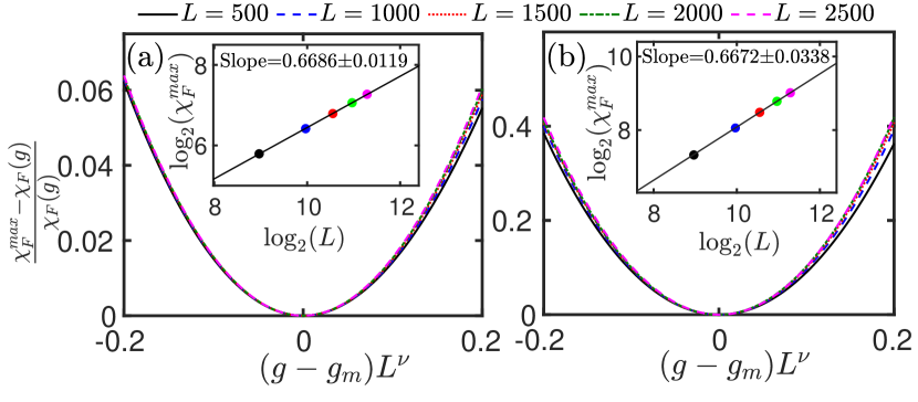
Figure 5: The finite size scaling for the fidelity susceptibility according to Eq. (11) for different system size $L$ for $U\rightarrow 1$ (a) and $U\rightarrow-1$ (b). $\Delta=0.5$. The corresponding size $L$ dependence of the maximum fidelity susceptibility $\chi_{F}^{max}$ is presented in the insets.

The insets of Fig. 5 show fidelity susceptibility at the maximum point as a function of the system size $L$ for both $U\rightarrow\pm 1$ on a log-log scale. A nice power law behavior $\chi_{F}^{max}\propto L^{\mu}$ is shown in both cases. The scaling exponent $\mu$ fitted from the numerical data at large $L$ tends to $2/3$.

In terms of the finite size scaling ansatz in Eq. (11), the critical exponents should satisfy the scaling law as $\mu/\nu=\alpha$, where $\alpha$ is just the fidelity susceptibility critical exponent. Obviously, $\alpha=2$ here is the same as the independent calculation given in Fig. 4, as well as the analytical derivation in the Appendix A.

V Finite-Truncation Effects on the criticality

The numerical solution of the RSM model requires one additional finite size parameter, namely the truncation of the bosonic Hilbert space. Does this truncation lead to additional critical exponents? In this section, we will demonstrate the solely effect of the photonic truncation $N_{tr}$ on the criticality of the RSM at $U=\pm 1$ by directly diagonalizing the RSM.

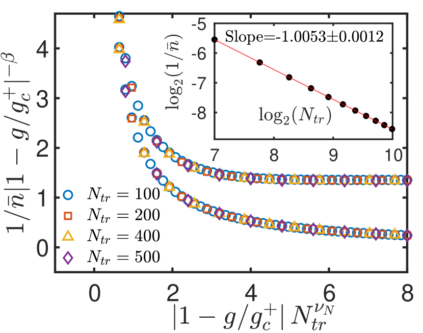
Figure 6: (a) Finite-size effects for the order parameter $1/\bar{n}$ in terms of the Hilbert space truncation according to Eq. (12) for both above and below the critical point. Inset: the corresponding log-log plot of $N_{tr}$ and $1/\bar{n}$ with fitting slope close to $-1$.

Using $N_{tr}$ as the alternative finite-size parameter, we first perform the finite-truncation scaling analysis on the RSM for the order parameter $1/\bar{n}$, and calculate the critical scaling exponents. Inset of Fig. 6 presents the order parameter $1/\overline{n}$ as a function of the photon truncation $N_{tr}$ right at the critical coupling strength on a log-log scale by numerics.  A nice power law behavior satisfying $1/\bar{n}\propto N_{tr}^{-\gamma_{N}}$ with $\gamma_{N}$ very close to $1$ is demonstrated. Interestingly, the critical scaling exponent in terms of the bosonic truncation number is different from that $\gamma=1/3$ in terms of the effective system size $L$ defined in (5) found in the Sec. III. By comparing the two size exponents of the order parameter, it is quite intriguing to note that two effective sizes can be related through $N_{tr}\propto L^{1/3}$.

The finite-truncation scaling function for order parameter is just similar to Eq. (7) by taking $N_{tr}$ as the system size as following

$$M=|1-g/g_{c}^{+}|^{\beta}f_{N}(|1-g/g_{c}^{+}|N_{tr}^{{\gamma_{N}/\beta}}),$$ (12)

Correspondingly, $\nu_{N}=\gamma_{N}/\beta$ denotes the correlation length exponent in terms of the bosonic truncation number $N_{tr}$ due to the scaling function. By numerics, we can also present the finite-truncation scaling according to Eq. (12) for different values of $N_{tr}$ above and below the critical point at $U=1$ in Fig. 6. Employing two exponents $\beta=1$ and $\gamma_{N}=1$ obtained independently above, we also observe that the scaling functions for different $N_{tr}$ collapse to the single curve, exhibiting an perfect universal scaling behavior. It follows that a universal critical behavior can be also established in terms of the bosonic Hilbert space truncation number, but leading to an alternative critical correlation length exponent of the RSM, $\nu_{N}=1$.

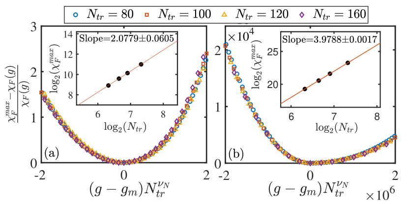
Figure 7: Finite-size effects for the fidelity susceptibility of the RSM and the quantum Rabi model in terms of Hilbert space truncation. Inset: the corresponding log-log plot of $N_{tr}$ and $\chi_{F}^{max}$ with fitting slope close to $2$. $U=1,\Delta=0.5$.

Then we turn to the finite-truncation scaling of the average fidelity susceptibility using $N_{tr}$. The corresponding scaling ansatz can be given by Eq. (11) if $L$ is replaced by $N_{tr}$. Figure  7 (a) show excellent universal scaling for large $N_{tr}$ with the correlation length exponent $\nu_{N}=1$. The inset exhibits a very good power law behavior $\chi_{F}^{max}\propto N_{tr}^{\mu_{N}}$ with $\mu_{N}=2$. These scaling exponents are also different from those in terms the size $L$ defined in Eq. (5).

Table 1: Summary of the critical exponents and the critical scaling exponents in the Rabi-Stark model. The critical exponent: $A\propto\left|g-g_{c}\right|^{y}$, the scaling exponents: $A\propto L^{y_{L}}$ in $L$, and $A\propto\left(N_{tr}\right)^{y_{N}}$ in $N_{tr}$, respectively.

exponent	$\varepsilon$	$1/\overline{n}$	$\Delta x$	$\chi_{F}$
$y$	2	1	-1/2	-2
$y_{L}$	-2/3	-1/3	1/6	2/3
$y_{N}$	-2	-1	1/2	2

At this stage, we may collect critical exponents and critical scaling exponents for more observables for completeness, which are summarized in Table I. The scaling exponents for the energy gap $\varepsilon$ and the variance of position quadrature of the field $\Delta x$ are calculated in the Appendix B. For an unified description, the critical exponent is defined by $A\propto\left|g-g_{c}\right|^{y}$, the finite-size scaling exponents by $A\propto L^{y_{L}}$, and the finite-truncation scaling exponent by $A\propto\left(N_{tr}\right)^{y_{N}}$, respectively, where $y$’s stand for the corresponding exponents of the observables $A$. One can note that all ratios of two scaling exponents $y_{L}/y_{N}$ are $1/3$, providing the consistent evidence for $N_{tr}\propto L^{1/3}$. The correlation length exponents $\nu=1/3$ in $L$ and $\nu_{N}=1$ in $N_{tr}$ can be seen by the ratios between the critical exponent and the scaling exponent, i.e. $y/y_{L}$ and $y/y_{N}$, for all observables.

Finally, for comprehensive comparisons, we revisit the criticality of the QRM by exploring the effects of the Hilbert space truncation. For brevity, we only analyze the finite-truncation scaling of the average fidelity susceptibility, which is independent of the order parameter. To facilitate the analysis of the criticality of the QRM, we set $L_{R}=\Delta/\omega=10^{8}$. In this case, the critical coupling of the QPT plenio2015 is around $\allowbreak 5000\omega$. Fig. 7 (b) show excellent universal scaling for large $N_{tr}$ with the correlation length exponent $\nu_{N}^{R}=2$ for the QRM. The inset show a very good power law behavior $\chi_{F}^{max}\propto N_{tr}^{\mu_{N}^{R}}$ with $\mu_{N}^{R}=4$. Very importantly, we can find that in terms of the same Hilbert space truncation, the critical correlation length exponent for the RSM is different from that in the QRM, indicating the different universality class.

Interestingly, comparing to the previous critical correlation length exponent $\nu^{R}=2/3$ in the QRM by the universal scaling of the same fidelity susceptibility using $L_{R}=\Delta/\omega$  Wei2018 , it is quite intriguing to note that two sizes in the QRM can be also related through $N_{tr}\propto L_{R}^{1/3}$. Comparing the effects of the Hilbert space truncations on both the RSM and QRM, we can see that the length defined in Eq. (5) of the RSM plays the equivalent role as the effective length $L_{R}=\Delta/\omega$ in the QRM. However, with these two equivalent length scales, the critical correlation length exponent $\nu=1/3$ of the RSM obtained in the last section is also different from $\nu^{R}=2/3$ in the QRM.

Using the atomic number, the finite-size scaling analysis for the fidelity susceptibility has been performed for the Dicke model  Liu2009 , and the correlation length exponent is obtained to be $2/3$, which is the same as that in Lipkin-Meshkov-Glick model Kwok2008 and the QRM using the effective size $L_{R}=\Delta/\omega$ Wei2018 . It is now generally accepted that the effective size $L_{R}=\Delta/\omega$ in the QRM plays the same role on the criticality as the atomic numbers of the Dicke model and the Lipkin-Meshkov-Glick model. No any different critical behavior of the continuous QPT has been observed in the Dicke model, Lipkin-Meshkov-Glick model, as well as the QRM in the infinite frequencies ratio. However, we indeed find that the critical correlation length exponent in the RSM is truly exceptional to all these models. Therefore, we believe that the RSM is in a different universality class.

VI Summary

We reveal the second-order QPT in the RSM at $U=\pm 1$ by studying the critical behavior of the energy gap, the order parameter, and the fidelity in this paper. The critical exponents for several observables can be analytically obtained. The energy gap exponent is $z\nu_{x}=2$ with $\nu_{x}=1/2$, in sharp contrast to $z\nu_{x}=1/2$ with $\nu_{x}=1/4$ in both the Dicke model  and the QRM. The critical exponent of the inverse photon number, which can be regarded as the order parameter of the RSM, is $\beta=1$, and the critical exponent of fidelity susceptibility is $\alpha=2$. All these critical exponents have also been confirmed by the numerically diagonalizing the RSM.

By using the effective system size $L=1/\left(1\mp U\right)$ for $U\rightarrow\pm 1$, the finite size scaling analyses for both the order parameter and the fidelity susceptibility are performed, and the universal scaling behaviors are clearly demonstrated. The size scaling exponent of the order parameter is found to be $\gamma=1/3$. Two size exponents of the fidelity susceptibility are also obtained by the perfect finite size scaling, which ratio recover the size independent critical exponent of the fidelity susceptibility $\alpha=2$. The finite size scaling analyses for the energy gap $\varepsilon$ and the variance of position quadrature of the field $\Delta x$ are also presented. The critical correlation exponent $\nu=1/3$ is obtained consistently in the calculation of all observables. A consistent picture is achieved and provides a strong evidence of the second-order QPT in the RSM.

We also explore the effects of the truncation of the bosonic Hilbert space on the criticality of the RSM. The finite-truncation scaling analyses for the several observables including the order parameter and the fidelity susceptibility are performed.  Alternative critical scaling exponents in terms of the photonic truncation number $N_{tr}$ are found. The universal critical behavior can be also established in terms of the truncation number. In particular, the corresponding critical correlation length exponent is $\nu_{N}=1/3$ in the RSM. Comparing with the scaling exponents obtained in the effective system size $L$, we can find $N_{tr}\propto L^{1/3}$.

To compare to the criticality of the QRM at infinite frequency ratio on the same foot, we also perform the finite-truncation scaling analysis for the order parameter independent fidelity susceptibility in the QRM. We find that the critical correlation length exponent in the RSM is different from $\nu_{N}^{R}=2/3$ in the QRM, suggesting that these two models would belong to different universality classes.

We like to point out that the QPT found in the RSM is of practical importance in two aspects.  One is that we do not need the extreme condition for the occurrence of the second-order QPT like the infinite ratio of the qubit and cavity frequencies $\Delta/\omega$ in the QRM.  In the present RSM, the frequency ratio $\Delta/\omega$ allowed for phase transitions can be any values. The other one is that for $U$ identical to the cavity frequency, the critical coupling is $g_{c}^{+}=\sqrt{(1-\Delta)/2}$, which can be extremely weak near the resonance by tuning the qubit frequency. This QPT should be experimentally feasible in any cavity-atom coupling device, such as the cavity (circuit) QEDs and the ion-trap. The price that should be paid is to incorporate the nonlinear Stark coupling between the two-level system and the fields in the devices.

ACKNOWLEDGEMENTS This work is supported by the National Science Foundation of China (Nos. 11674285, 11834005), the National Key Research and Development Program of China (No. 2017YFA0303002).

^∗ Corresponding author. Email:qhchen@zju.edu.cn.

Appendix A Analytical derivation of some critical exponents of the RSM at $U=1$

In this Appendix, we derive some critical exponent analytically based on the analytical exact solutions to the RSM at $U=1$. We will first briefly review the previous solution in the framework of the Fock space xieCTP , then we present the exact eigenfunction.

In terms of the basis of $\sigma_{z}$, the Hamiltonian (1) in the matrix form can be written as

$$H_{0}=\left(\begin{array}[]{cc}2a^{{\dagger}}a+\frac{\Delta}{2}&g\left(a^{{\dagger}}+a\right)\\ g\left(a^{{\dagger}}+a\right)&-\frac{\Delta}{2}\end{array}\right).$$ (13)

The series expansion of the eigenfunction in the Fock space is

$$\left|\Psi\right\rangle=\binom{\left|\Psi_{1}\right\rangle}{\left|\Psi_{2}\right\rangle}=\left(\begin{array}[]{c}\sum_{n}^{\infty}e_{n}\left|\phi_{n}\right\rangle\\ \sum_{n}^{\infty}f_{n}\left|\phi_{n}\right\rangle\end{array}\right).$$ (14)

where $e_{n}$ and $f_{n}$ are the expansion coefficients, $\left|\phi_{n}\right\rangle$ is the number states. The Schrödinger equation then gives

$$\left(2a^{{\dagger}}a+\frac{\Delta}{2}\right)\sum_{n}^{\infty}e_{n}\left|\phi_{n}\right\rangle+g\left(a^{{\dagger}}+a\right)\sum_{n}^{\infty}f_{n}\left|\phi_{n}\right\rangle$$ (15)

$$= E\sum_{n}^{\infty}e_{n}\left|\phi_{n}\right\rangle,$$

$$g\left(a^{{\dagger}}+a\right)\sum_{n}^{\infty}e_{n}\left|\phi_{n}\right\rangle=\left(\frac{\Delta}{2}+E\right)\sum_{n}^{\infty}f_{n}\left|\phi_{n}\right\rangle.$$ (16)

By inspection of Eq. (16), we obtain

$$\sum_{n}^{\infty}f_{n}\left|\phi_{n}\right\rangle=\frac{g\left(a^{{\dagger}}+a\right)}{\frac{\Delta}{2}+E}\sum_{n}^{\infty}e_{n}\left|\phi_{n}\right\rangle,$$

Inserting it into Eq. (15) leads to the effective Hamiltonian for the bosonic wavefunction in the upper level $\left|\Psi_{1}\right\rangle$

$$H_{eff}=2a^{\dagger}a+\chi(a^{\dagger}+a)^{2}+\frac{\Delta}{2},$$ (17)

with $\chi=\frac{g^{2}}{\frac{\Delta}{2}+E}$.

To diagonalize the Hamiltonian above, we apply the squeezing transformation $S=\exp{[\frac{r}{2}(a^{2}-{a^{\dagger}}^{2})]}$ with $r=\frac{1}{4}\ln(\frac{1}{1+2\chi})$, and then get a Hamiltonian for a quantum oscillator

$$H^{\prime}=SH_{eff}S^{\dagger}=\sqrt{1+2\chi}(2a^{\dagger}a+1)-1+\frac{\Delta}{2}.$$ (18)

The eigenenergy $E$ is obviously given by

$$E=\sqrt{1+2\chi}(2n+1)-1+\frac{\Delta}{2},\quad n=0,1,2...\infty.$$ (19)

which further results in Eq. (2).

The eigenfunction to the harmonic oscillator is just the Fock state $\left|n\right\rangle$, thus the eigenfunction for the RSM at $U=1$ for the low spectra reads

$$\left|\Psi_{n}\right\rangle=\frac{1}{N_{n}}\begin{pmatrix}c_{n}S^{\dagger}\left|n\right\rangle\\ d_{n}S^{\dagger}(a^{\dagger}+a)\left|n\right\rangle\end{pmatrix}$$ (20)

where $c_{n}=(1+2\chi_{n})^{1/4}$ and $d_{n}=\chi_{n}/g$, and the normalization factor $N_{n}=\sqrt{c_{n}^{2}+(2n+1)d_{n}^{2}}$. Several quantities can be calculated using this eigenfunction. For convenience, we denote the dimensionless coupling parameter $\lambda=g/g_{c}^{+}$.

First, we calculate the mean photon number using the wave function of Eq. (20) as

$$\left\langle a^{\dagger}a\right\rangle = \frac{1}{N_{n}^{2}}[c_{n}^{2}\left\langle n\right|Sa^{\dagger}aS^{\dagger}]\left|n\right\rangle$$ (21)

$$+d_{n}^{2}\left\langle n\right|(a^{\dagger}+a)Sa^{\dagger}aS^{\dagger}(a^{\dagger}+a)\left|n\right\rangle]$$

$$= \frac{1}{N_{n}^{2}}\{c_{n}^{2}(n\cosh 2r+\sinh^{2}r)$$

$$+d_{n}^{2}[\left(2n^{2}+n+1\right)\cosh 2r+(2n+1)\sinh^{2}r$$

$$+n(n+1)\sinh 2r]\}$$

$$= \frac{3}{8}\frac{(2n+1)^{2}+1}{(1-\Delta)(1-\lambda^{2})}-\frac{1}{2}\left[1-(1-\Delta)\lambda^{2}\right]$$

$$\simeq \frac{3}{8}\frac{(2n+1)^{2}+1}{(1-\Delta)(1-\lambda^{2})}\propto(1-\lambda)^{-1}.$$

where the limit $g\rightarrow g_{c}$, i. e. $\lambda$ is a small quantity, is performed in the last step. This is just Eq. (6) for the order parameter in the main text.

Then we turn to the variance of position quadrature of the field $\Delta x$. By using $x=1/\sqrt{2}(a^{\dagger}+a)$ , we have

$$(\Delta x)^{2} = \left\langle x^{2}\right\rangle-\left\langle x\right\rangle^{2}=\frac{1}{2}\left\langle(a^{\dagger}+a)^{2}\right\rangle$$ (22)

$$= \frac{e^{2r}}{2N_{n}^{2}}\left[c_{n}^{2}(2n+1)+d_{n}^{2}(6n^{2}+6n+3)\right]$$

$$\simeq \frac{3\left[(2n+1)^{2}+1\right]}{4(1-\Delta)\left(1-\lambda^{2}\right)}\propto(1-\lambda)^{-1}.$$

The critical exponent $\nu_{x}=1/2$ for the position fluctuation is obtained, which is part of the gap exponent in the main text. The relative difference for the mean photon number and the position is within $2\%$ at $\lambda=0.9$.

Finally we calculate the ground state fidelity susceptibility $\chi_{F}$ in the limit of $g\rightarrow g_{c}^{+}$, by using its the differential form Eq. (10). The eigenfunction of n-th energy level in this limit can be written as

$$\left|\Psi_{n}\right\rangle=\begin{pmatrix}C_{n}S^{\dagger}\left|n\right\rangle\\ D_{n}S^{\dagger}(a^{\dagger}+a)\left|n\right\rangle\end{pmatrix},$$ (23)

where

$$C_{n}=\frac{c_{n}}{N_{n}} = \frac{c_{n}}{\sqrt{c_{n}^{2}+(2n+1)d_{n}^{2}}}$$

$$= \frac{\sqrt{1+2\chi}}{\sqrt{\sqrt{1+2\chi}+(2n+1)\chi^{2}/g^{2}}}$$

$$\simeq \frac{(1-\Delta)\lambda}{2n+1}\sqrt{2(1-\lambda^{2})}$$

$$D_{n}=\frac{d_{n}}{N_{n}} = \frac{d_{n}}{\sqrt{c_{n}^{2}+(2n+1)d_{n}^{2}}}$$

$$= \frac{\chi/g}{\sqrt{\sqrt{1+2\chi}+(2n+1)\chi^{2}/g^{2}}}$$

$$\simeq \sqrt{\frac{1}{2n+1}}$$

Now, we can calculate the first-order partial derivative of the ground state wave function with respect to $\lambda$

$$\left|\frac{\partial\Psi_{0}}{\partial\lambda}\right\rangle=\begin{pmatrix}(\frac{\partial C_{0}}{\partial\lambda})S^{\dagger}+C_{0}(\frac{\partial S^{\dagger}}{\partial\lambda})\left|0\right\rangle\\ D_{0}(\frac{\partial S^{\dagger}}{\partial\lambda})(a^{\dagger}+a)\left|0\right\rangle\end{pmatrix},$$

where

$$\frac{\partial S^{\dagger}}{\partial\lambda}=-\frac{1}{2}\frac{\partial r(\lambda)}{\partial\lambda}S^{\dagger}(a^{2}-{a^{\dagger}}^{2})$$ (24)

$$\frac{\partial r}{\partial\lambda}=-\frac{1}{2(1+2\chi)}\frac{\partial\chi}{\partial\lambda}\simeq\frac{\lambda}{1-\lambda^{2}}.$$ (25)

Some overlaps in Eq. (10) are list below after lengthy calculation

$$\left\langle\frac{\partial\Psi_{0}}{\partial\lambda}\bigg{|}\frac{\partial\Psi_{0}}{\partial\lambda}\right\rangle = \left(\frac{\partial C_{0}}{\partial\lambda}\right)^{2}+\frac{C_{0}^{2}}{2}\left(\frac{\partial C_{0}}{\partial\lambda}\right)+\frac{3D_{0}^{2}}{2}\left(\frac{\partial C_{0}}{\partial\lambda}\right)^{2}$$ (26)

$$\simeq \frac{(1-\Delta)^{2}\left(2+\lambda^{4}\right)}{\left(1-\lambda^{2}\right)}+\frac{3\lambda^{2}}{2\left(1-\lambda^{2}\right)^{2}},$$

$$\left\langle\Psi_{0}\bigg{|}\frac{\partial\Psi_{0}}{\partial\lambda}\right\rangle = \left\langle\Psi_{0}\bigg{|}\frac{\partial\Psi_{0}}{\partial\lambda}\right\rangle=C_{0}\frac{\partial C_{0}}{\partial\lambda}$$ (27)

$$\simeq -{2(1-\Delta)^{2}\lambda}.$$

We now arrive at the fidelity susceptibility in the limit to the critical point

$$\chi_{F} \simeq \frac{(1-\Delta)^{2}\left(2+\lambda^{4}\right)}{\left(1-\lambda^{2}\right)}+\frac{3}{2}\frac{\lambda^{2}}{\left(1-\lambda^{2}\right)^{2}}+4(1-\Delta)^{2}\lambda^{2}$$ (28)

$$\simeq \frac{3}{2}\frac{\lambda^{2}}{\left(1-\lambda^{2}\right)^{2}}\propto(1-\lambda)^{-2},$$

which explicitly yields the critical exponent for the fidelity susceptibility as $\alpha=2$. The relative difference is within $4\%$ at $\lambda=0.99$.

Appendix B Finite-size scaling for the energy gap $\varepsilon$ and the variance of position quadrature of the field $\Delta x$

The finite-size scaling function near critical point $g_{c}^{+}$ at $U=1$ for any observable $A$ should satisfy following form

$$A(\mathbb{L},g)=|1-g/g_{c}^{+}|^{\beta}f(|1-g/g_{c}^{+}|\mathbb{L}^{\nu^{\prime}})$$ (29)

where $\nu^{\prime}$ is the critical correlation length exponent, the size $\mathbb{L}$ could be either the effective system size $L$ defined in Eq. (5) or the Herbert space truncation $N_{tr}$. Accordingly, the critical exponent $\nu^{\prime}$ is either $\nu$ in terms of $L$ or $\nu_{N}$ in $N_{tr}$.

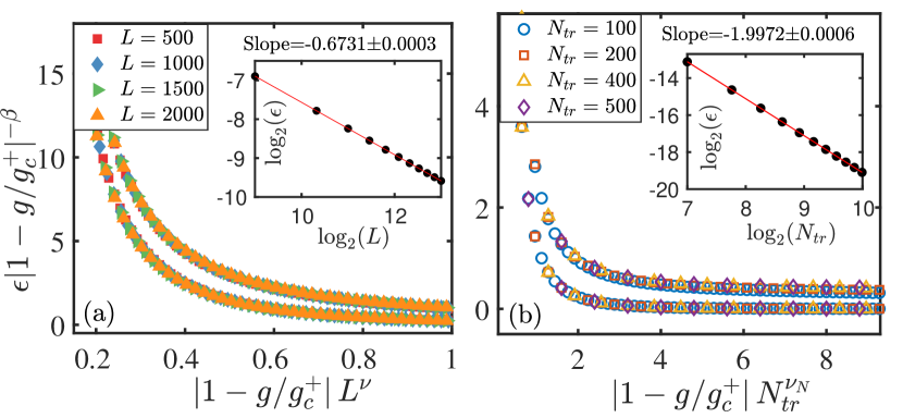
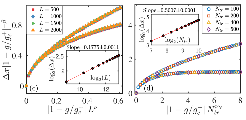
Figure 8: Finite size scaling for the energy gap $\epsilon$ (upper panel) and the variance of position quadrature of the field $\Delta x$ (lower panel) according to Eq. (29) in terms of $\mathbb{L}$ for both above and below the critical point. The corresponding inset displays the log-log plot of $\epsilon$ ($\Delta x$ ) and $\mathbb{L}$. $\mathbb{L}=L$ for left panel and $\mathbb{L}=N_{tr}$ at $U=1$ for right panel. $\Delta=0.5.$

Here we analyze the finite-size scaling for the energy gap $\epsilon$ and the variance of position quadrature of the field $\Delta x\$ in terms of both the effective system size $L$ and the bosonic Hilbert space truncation $N_{tr}$ in Fig. 8 by diagoanlizing the RSM.  The insets of the upper panel of Fig. 8 show the energy gap $\epsilon$ as a function of $\mathbb{L}$ on a log-log scale by numerics.  A nice power law behavior is observed with slopes very close to $-2/3$ and $-2$, respectively. The insets of the lower panel of Fig. 8 is plotted for the variance of position quadrature of the field $\Delta x$, and the power law behavior gives the slops $1/6$ and $1/2$ in two sizes, respectively. For $\epsilon$, with the critical exponent obtained in the main text $\beta=2$ and the critical correlation length exponent $\nu^{\prime}=1/3$ and $1$ for the two size, the excellent collapse can be find in the upper panel of Fig. 8. Similarly, for $\Delta x$, the critical exponent obtained in the main text $\beta=-1/2$, using the same values of $\nu^{\prime}$ in the upper panel of Fig. 8, we also note the perfect collapse in the lower panel of Fig. 8.

References

- (1) P. W. Anderson. More Is Different. Science, 177, 393 (1972).
- (2) S. Sachdev, Quantum Phase Transitions, 2nd ed. (Cambridge University Press, Cambridge, England, 2011).
- (3) I. I. Rabi, Phys. Rev. 51, 652 (1937).
- (4) E. T. Jaynes and F. W. Cummings Proc. IEEE 51, 89(1963).
- (5) M.-J. Hwang, R. Puebla, and M. B. Plenio, Phys. Rev. Lett.115, 180404 (2015);
- (6) M.-J. Hwang and M. B. Plenio, Phys. Rev. Lett. 117,123602 (2016).
- (7) M. X. Liu, S. Chesi, Z. J. Ying, X. S. Chen, H. G. Luo, and H. Q. Lin, Phys. Rev. Lett.119, 220601 (2017).
- (8) D. Braak, Q. H. Chen, M. Batchelor, and E. Solano, J. Phys.A: Math. Gen. 49, 300301 (2016).
- (9) J. M. Raimond, M. Brune, and S. Haroche, Rev. Mod. Phys. 73, 565 (2001).
- (10) T. Niemczyk et al., Nature Physics 6, 772 (2010).
- (11) F. Yoshihara, T. Fuse, S. Ashhab, K. Kakuyanagi, S. Saito, and K. Semba, Nat. Phys. 13, 44 (2016).
- (12) P. Forn-Díaz, J. J. García-Ripoll, B. Peropadre, J. L. Orgiazzi, M. A. Yurtalan, R. Belyansky, C. M. Wilson, and A. Lupascu, Nat. Phys. 13, 39 (2016).
- (13) D. Leibfried, R. Blatt, C. Monroe, and D. Wineland, Rev. Mod. Phys. 75, 281 (2003).
- (14) J. Clarke and F. K. Wilhelm, Nature 453, 1031 (2008).
- (15) P. Forn-Díaz et al., Phys. Rev. Lett. 105, 237001 (2010).
- (16) J. Casanova, G. Romero, I. Lizuain, J. J. García-Ripoll and E. Solano, Phys. Rev. Lett. 105 263603 (2010).
- (17) A. L. Grimsmo and S. Parkins, Phys. Rev. A 87 033814 (2013).
- (18) A. L. Grimsmo and S. Parkins, Phys. Rev. A 89 033802 (2014).
- (19) A. J. Maciejewski, M. Przybylska, and T. Stachowiak, Phys. Lett. A 379 1503(2015).
- (20) H. P. Eckle and H. Johannesson, J. Phys. A: Math. Theor. 50, 294004 (2017).
- (21) Y. F. Xie, L. W. Duan, Q. H. Chen, J. Phys. A: Math. Theor. 52, 245304 (2019).
- (22) L. Cong, S. Felicetti, J. Casanova, L. Lamata, E. Solano, and I. Arrazola, Phys. Rev. A 101, 032350 (2020).
- (23) Y. F. Xie, X. Y. Chen, X. F. Dong, and Q. H. Chen, Phys. Rev. A 101, 053803(2020).
- (24) C. Emary and T. Brandes, Phys. Rev. E 67, 066203(2003); Phys. Rev. Lett. 90, 044101(2003).
- (25) W. L. You, Y. W. Li, and S. J. Gu, Phys. Rev. E 76, 022101 (2007).
- (26) S. J. Gu, H. M. Kwok,W. Q. Ning and H. Q. Lin, Phys. Rev. B, 77, 245109(2008).
- (27) H. M. Kwok, W. Q. Ning, S. J. Gu, and H. Q. Lin, Phys. Rev. E 78, 032103(2008).
- (28) S. J. Gu, Int. J. Mod. Phys. B 24, 4371 (2010).
- (29) T. Liu,Y. Y. Zhang,Q. H. Chen and K. L.,Wang, Phys. Rev. A 80, 023810(2009).
- (30) B. B. Wei and X. C. Lv, Phys. Rev. A.97, 013845(2018).
- (31) Y. F. Xie and Q. H. Chen, Commun. Theor. Phys. 71 623 (2019).