First-order differentiability properties of a class of equality constrained optimal value functions with applications

Abstract

In this paper we study the right differentiability of a parametric infimum function over a parametric set defined by equality constraints. We present a new theorem with sufficient conditions for the right differentiability with respect to the parameter. Target applications are nonconvex objective functions with equality constraints arising in optimal control and shape optimisation. The theorem makes use of the averaged adjoint approach in conjunction with the variational approach of Kunisch, Ito and Peichl. We provide two examples of our abstract result: (a) a shape optimisation problem involving a semilinear partial differential equation which exhibits infinitely many solutions, (b) a finite dimensional quadratic function subject to a nonlinear equation.

1 Introduction

Let a normed space $X$, a vector space $Y$ and $\tau>0$ be given. In this paper we study the one-sided differentiability in $t=0^{+}$ of the optimal value-function

(1) $$t\mapsto g(t):=\inf_{u\in E(t)}f(t,u),$$

where $f:[0,\tau]\times X\to{\mathbf{R}}$ is a given function. The $E(t)$ denotes the set of states given by

(2) $$E(t)=\{u^{t}\in X:e(t,u^{t},\varphi)=0\quad\text{ for all }\varphi\in Y\},$$

where $e:[0,\tau]\times X\times Y\to{\mathbf{R}}$ is a function that is linear with respect to the last argument. The Lagrangian $(t,u,p)\mapsto G(t,u,p):[0,\tau]\times X\times Y\to{\mathbf{R}}$ associated with (1) is defined by

(3) $$G(t,u,q)=f(t,u)+e(t,u,q).$$

With this Lagrangian the set $E(t)$ can be expressed in terms of the Lagrangian $G$ as follows

(4) $$E(t)=\{u^{t}\in X:\partial_{p}G(t,u^{t},0)(\varphi)=0\;\text{ for all }\varphi\in Y\}$$

and $g$ can be written as a minimax (see [14])

(5) $$g(t)=\inf_{\varphi\in X}\sup_{\psi\in Y}G(t,\varphi,\psi)=\inf_{\varphi\in E(t)}G(t,\varphi,0).$$

We will provide new conditions (see Hypothesis (H3)) under which the function $g$ is right differentiable. The pertinence of the result is illustrated by applying it to a finite dimensional problem and a shape optimisation problem.

The problem of finding the right derivative of (1) arises naturally when deriving optimality conditions appearing in equality constrained finite and infinite dimensional control and shape optimisation problems. Accordingly it has been studied by many authors before and sufficient conditions, even with inequality constraints are known; see, e.g., the review article [4]. Often for inequality constrained problems suitable constraint qualifications (e.g. Robinson’s constraint qualification [32]) are required which impose a certain regularity on minimisers; see [24, 38, 29]. In [30] the right differentiability is examined in infinite dimensions under the assumption that the elements of $E(t)$ arise from convex optimisation problems; see also [33] and [2, 3] for results in infinite dimension.

In case $E(t)$ is independent of $t$ let us mention the early work of J. M. Danskin [8, 7] where a maximum function with respect to a parameter was studied. When the solution of the maximum problem (and similarly minimum problem) is not unique, then a natural non-differentiability arises. In this case only directional derivatives or sub-differentials are computable. We also refer to the monographs [17, 20, 31] and references therein. In the review article [4] and also the book chapters [5, Chap. 4] and [22, Chap. 2] several conditions for right differentiability of $g$ are given (see also references therein). In particular first and second order expansions of value functions are studied using second order conditions.

As mentioned before second order analysis can be used to obtain differentiability of the optimal solution $u^{t}$ and hence differentiability of the value function $g$. Let us mention [21] where the differentiability of the value function with respect to Dirichlet data of a tracking-type cost function constrained by a semilinear parabolic PDE is studied. A key ingredient is a Hölder estimate of order $1/2$ of the optimal control with respect to the Dirichlet data.

The differentiability of parametric minimax functions under saddle point assumptions has been studied in [6] by Correa and Seeger and was subsequently extended and applied to shape optimisation problems by Delfour and Zolésio in [15]. For nonlinear equality constraints this saddle point assumption is unfortunately often not satisfied.

In [35, 34] an approach to the differentiability of a minimax without a saddle point assumption for the Lagrangian was presented. An extension to the multivalued case can be found in [14, Thm. 4.1] and [12, Thm. 2 and Thm. 3]. In addition in [14, Thm. 3.1] and [12, Thm. 1] also the singleton case was revisited and extended by introducing an extra term. For applications to the single valued case of this approach we refer to [35] and also [25] and [36]. In this context let us also mention the approaches of [34, p.54, Thm. 4.6] and [10, Thm. 3.3] (see also [11]), where a Lagrangian approach using an unperturbed adjoint variable is proposed for the single-valued case. The adjoint method [10, Thm. 3.3] has also been recently used in [19] and [18] to compute topological derivatives and, in addition, also a thorough comparison with the averaged adjoint method is provided. From this it appears, at least in the context of computing topological derivatives, that the averaged adjoint method seems favorable, since a larger class of cost functionals could be treated. This may be rooted in the infinite dimensionality of the problem.

The key idea of the averaged adjoint approach is to replace the perturbed standard adjoint by the so-called averaged adjoint state equation. This allows to deal with non-convex objective functions and non-linear state equations. Let us also mention the variational approach of [23] where another approach is proposed to show the differentiability of a minimax by using some sort of second order expansion. Both approaches have in common that they bypass the computation of the derivative of the control-to-state operator. Although both approaches are from its nature very different we will show in this paper how they can effectively be combined to establish yet another even more powerful new theorem on the differentiability of the minimax.

Our result gives new easy to check conditions and generalises results in [14]. The target applications of our theorem are the shape sensitivity analysis yet the result can also be applied to optimal control problems in general.

Notation

Let $f:[0,\tau]\times\mathcal{U}_{1}\times\mathcal{U}_{2}\rightarrow{\mathbf{R}}$ be a function defined on the Cartesian product of the interval $[0,\tau]$, $\tau>0$ and the open subsets $\mathcal{U}_{1}\subset X$ and $\mathcal{U}_{2}\subset Y$ of normed spaces. Then we define for $(t,u,p)\in[0,\tau)\times\mathcal{U}_{1}\times\mathcal{U}_{2}$ and $v\in X$ and $w\in Y$ the following one sided directional derivatives

(6) $$\begin{split}\partial_{t}f(t,u,p)&:=\lim_{h\searrow 0}\frac{f(t+h,u,p)-f(t,u,p)}{h},\\ \partial_{u}f(t,u,p)(v)&:=\lim_{h\searrow 0}\frac{f(t,u+hv,p)-f(t,u,p)}{h},\\ \partial_{p}f(t,u,p)(w)&:=\lim_{h\searrow 0}\frac{f(t,u,p+hw)-f(t,u,p)}{h},\end{split}$$

provided the limits on the right hand side exist, respectively. The notation $h\searrow 0$ indicates that $h\rightarrow 0$ under the condition $h>0$.

We equip ${\mathbf{R}}^{d}$ with the Euclidean norm $\|\cdot\|$ and denote by $\|A\|$ the corresponding operator norm for $A\in{\mathbf{R}}^{d\times d}$.

Throughout the paper, we will use the terminology state equation and adjoint state equation.

2 Minimax theorem via the averaged adjoint equation

2.1 Averaged adjoint equation

Let $X,Y$ and $G$ be as in the introduction. We will henceforth assume that $g(t)$ is finite for all $t\in[0,\tau]$.

Definition 2.1.

We introduce for $t\in[0,\tau]$ the set of minimisers

(7) $$X(t):=\{u^{t}\in E(t):\;\inf_{u\in E(t)}f(t,u)=f(t,u^{t})\}.$$

Notice that $X(t)\subset E(t)$ and that $X(t)=E(t)$ whenever $E(t)$ is a singleton. However, in general $X(t)$ and $E(t)$ do not need to coincide. The definition of the averaged adjoint equation requires that the set of states is not empty:

Assumption (H0).

For all $t\in[0,\tau]$ we have $X(t)\not=\emptyset$.

Before we can introduce the averaged adjoint equation we need the following hypothesis.

Assumption (H1).

For all $t\in[0,\tau]$ and $(u^{0},u^{t})\in X(0)\times E(t)$ we assume:

1. For all $p\in Y$, the mapping $s\mapsto G(t,su^{t}+(1-s)u^{0}),p):[0,1]\to{\mathbf{R}}$ is absolutely continuous.

2. For all $(\varphi,q)\in X\times Y$ and almost all $s\in(0,1)$ the function

   (8) $$s\mapsto\partial_{u}G(t,su^{t}+(1-s)u^{0},p)(\varphi):[0,1]\to{\mathbf{R}}$$

   is well-defined and belongs to $L_{1}(0,1)$.

Remark 2.2.

Notice that item (i) implies that for all $t\in[0,\tau]$, $(u^{0},u^{t})\in X(0)\times E(t)$ and $p\in Y$,

(9) $$G(t,u^{t},p)=G(t,u^{0},p)+\int_{0}^{1}\partial_{u}G(t,su^{t}+(1-s)u^{0},p)(u^{t}-u^{0})\,ds.$$

This follows at once by applying the fundamental theorem of calculus to $s\mapsto G(t,su^{t}+(1-s)u^{0},p)$ on $[0,1]$.

The following gives the definition of the adjoint and averaged adjoint equation; see [35].

Definition 2.3 (Averaged adjoint equation).

Let $\tilde{X}\subset X$ be a linear subspace. Given $t\in[0,\tau]$ and $(u^{0},u^{t})\in E(0)\times E(t)$, the averaged adjoint state equation is defined as follows: find $q^{t}\in Y$, such that

(10) $$\int_{0}^{1}\!\!\partial_{u}G(t,su^{t}+(1-s)u^{0},q^{t})(\varphi)\,ds=0\quad\text{ for all }\varphi\in\tilde{X}.$$

For every triplet $(t,u^{0},u^{t})$ the set of solutions to (10) is denoted by $Y(t,u^{0},u^{t})$.

Definition 2.4.

The standard adjoint $p^{t}\in X$ is defined by $\partial_{u}G(t,u^{t},p^{t})(\varphi)=0$ for all $\varphi\in\tilde{X}$ and the set of adjoints associated with $(t,u^{t})$ is denoted $Y(t,u^{t})$.

Notice that $Y(0,u^{0})=Y(0,u^{0},u^{0})$ for all $u^{0}\in E(0)$, that is, the averaged adjoint equation reduces to the usual adjoint equation. The averaged adjoint equation allows us to express the Lagrangian at time $t$ solely through the Lagrangian evaluated at $(t,u^{0},q^{t})$.

Lemma 2.5.

Let $t\in(0,\tau]$. Then for all $(u^{0},u^{t})\in E(0)\times E(t)$ with $u^{t}-u^{0}\in\tilde{X}$, and $q^{t}\in Y(t,u^{0},u^{t})$, we have

(11) $$G(t,u^{t},q^{t})=G(t,u^{0},q^{t}).$$

Proof 2.6.

This follows directly from Remark 2.2 noting that $u^{t}-u^{0}\in\tilde{X}$ is an admissible test function in (10) and hence the last term in (9) vanishes.

Remark 2.7.

Notice that (11) holds for all $t>0$, but not necessarily at $t=0$. The reason behind this is a discontinuity at $t=0$. Let $u^{t}\in E(t)$ and $\bar{u}^{0}\in E(0)$ with $u^{0}\neq\bar{u}^{0}$ and let $q^{t}\in Y(t,\bar{u}^{0},u^{t})$. Set $f_{1}(t):=G(t,u^{t},q^{t})$ and $f_{2}(t):=G(t,\bar{u}^{0},q^{t})$ for $t\in[0,\tau]$. Then from (11) we obtain

(12) $$f_{1}(t)=f_{2}(t)\quad\text{ for all }t>0,$$

but $f_{1}$ and $f_{2}$ do not coincide at $t=0$ unless $f_{1}(0)=f(0,u^{0})=f(0,\bar{u}^{0})=f_{2}(0)$. However, if we also let $\bar{u}^{0}_{t}\in E(0)$, such that $\bar{u}^{0}_{0}=u^{0}$, then the functions $f_{1}(t):=G(t,u^{t},q^{t})$ and $f_{2}(t):=G(t,\bar{u}^{0}_{t},q^{t})$ will coincide at $t=0$. This observation is important for our main theorem (Theorem 2.12); see also Hypothesis (H3).

Corollary 2.8.

For all $t\in(0,\tau]$, $(u^{0},u^{t})\in E(0)\times X(t)$ with $u^{t}-u^{0}\in\tilde{X}$, and for all $q^{t}\in Y(t,u^{0},u^{t})$, we have

(13) $$g(t)=G(t,u^{t},q^{t})=G(t,u^{0},q^{t}).$$

Proof 2.9.

Let $t\in(0,\tau]$, $(u^{0},u^{t})\in E(0)\times X(t)$, and $q^{t}\in Y(t,u^{0},u^{t})$ be given. Since $u^{t}\in X(t)$ we obtain by definition

(14) $$g(t)=\inf_{u\in E(t)}G(t,u,0)=G(t,u^{t},0).$$

On the other hand since $X(t)\subset E(t)$, we have $u^{t}\in E(t)$ and thus $G(t,u^{t},0)=G(t,u^{t},q^{t}).$ Now we can apply Lemma 2.5 to obtain

(15) $$G(t,u^{t},q^{t})=G(t,u^{0},q^{t}).$$

Finally (14) and (15) together imply (13).

Remark 2.10.

Notice that in our setting the test space of the adjoint and averaged adjoint equation might be smaller than the space of definition of the parametrised Lagrangian, that is, $\tilde{X}\neq X$ in general. This is for instance the case when solving the Dirichlet Laplacian where the test space would be $H^{1}_{0}$ and the trial space $H^{1}$. We refer to the last section for an example.

Remark 2.11.

Let $G:[0,\tau]\times X\times Y\rightarrow{\mathbf{R}}$ be a Lagrangian and $u\in X$. Assume that $\partial_{t}G(0,u,p)$ exists for all $p\in Y$. Then $p\mapsto\partial_{t}G(0,u,p):Y\rightarrow{\mathbf{R}}$ is affine.

2.2 A new minimax theorem for Lagrangians

The next theorem gives new sufficient conditions for $g$ to be right differentiable at $t=0$. Our theorem extends [6] and complements [14, Theorem 4.1] for functions $G$ that are Lagrangians. We will give a new theorem which provides new sufficient conditions for which the limit

(16) $$dg(0):=\lim_{t\searrow 0}\frac{g(t)-g(0)}{t}$$

exists, where $g$ is given by (1).

Theorem 2.12.

Let $G$ be a Lagrangian and suppose that Hypotheses (H0)–(H1) and the following conditions are satisfied.

1. For all $u\in X(0)$ and all $p\in Y(0,u)$, $\partial_{t}G(0,u,p)$ exists;

2. For every null-sequence $(t_{n})$, $t_{n}\in(0,\tau]$, there exist $u^{0}\in X(0)$ and $p^{0}\in Y(0,u^{0})$, a subsequence $(t_{n_{k}})$, elements $(u^{0}_{t_{n_{k}}},u^{t_{n_{k}}})\in E(0)\times X(t_{n_{k}})$, $u^{t_{n_{k}}}-u^{0}_{t_{n_{k}}}\in\tilde{X}$ and $q^{t_{n_{k}}}\in Y(t_{n_{k}},u^{0}_{t_{n_{k}}},u^{t_{n_{k}}})$, such that

   $$\liminf_{k\to\infty}\frac{G(t_{n_{k}},u^{0}_{t_{n_{k}}},q^{t_{n_{k}}})-G(0,u^{0}_{t_{n_{k}}},q^{t_{n_{k}}})}{t_{n_{k}}}\geq\partial_{t}G(0,u^{0},p^{0}).$$

3. For every $u^{0}\in X(0)$ there is a suboptimal path $t\mapsto\bar{u}^{t}:[0,\tau]\rightarrow X$ satisfying, $\bar{u}^{0}=u^{0}$, $\bar{u}^{t}-u^{0}\in\tilde{X}$, $\bar{u}^{t}\in E(t)$ and

   $$\lim_{t\searrow 0}\frac{\|\bar{u}^{t}-u^{0}\|_{X}}{t^{1/2}}=0$$

   and for all $p^{0}\in Y(0,u^{0})$,

   (17) $$\limsup_{t\searrow 0}\frac{G(t,\bar{u}^{t},p^{0})-G(0,\bar{u}^{t},p^{0})}{t}\leq\partial_{t}G(0,u^{0},p^{0}).$$

4. For every $u^{0}\in X(0)$ and every $p^{0}\in Y(0,u^{0})$,

   (18) $$|G(0,u,p^{0})-G(0,u^{0},p^{0})-\partial_{u}G(0,u^{0},p^{0})(u-u^{0})|=\mathcal{O}(\|u-u^{0}\|^{2}_{X}).$$

Then the one sided derivative $dg(0)$ exists and we find $u^{0}\in X(0)$ and $p^{0}\in Y(0,u^{0})$, such that

(19) $$dg(0)=\partial_{t}G(0,u^{0},p^{0})$$

and we have the bound

(20) $$\inf_{u\in X(0)}\inf_{p\in Y(0,u)}\partial_{t}G(0,u,p)\leq dg(0)\leq\inf_{u\in X(0)}\sup_{p\in Y(0,u)}\partial_{t}G(0,u,p).$$

If, in addition, for all $u\in X(0)$ the set $Y(0,u)=\{p^{0}(u)\}$ is a singleton, then

(21) $$dg(0)=\inf_{u\in X(0)}\partial_{t}G(0,u,p^{0}(u))=\partial_{t}G(0,u^{0},p^{0}).$$

Before we turn our attention to the proof of this theorem let us make a few remarks.

Remark 2.13.

Let us give a guideline on how Hypothesis (H3) can be verified in practice. Let a null-sequence $(t_{n})$ and $(u^{t_{n}})\in X(t_{n})$ be given. Typically one can use compactness arguments to find $u^{0}\in X(0)$ and a subsequence (denoted the same) such that $u^{t_{n}}\to u^{0}$ in some topology on $X$ (e.g. weak or strong). Then one constructs $u^{t_{n}}_{0}\in E(0)$, such that $u^{t_{n}}_{0}\to u^{0}$ and $Y(t_{n},u^{t_{n}}_{0},u^{t_{n}})\neq\emptyset$. Then it only remains to verify that there is a sequence $q^{t_{n}}\in Y(t_{n},u^{t_{n}}_{0},u^{t_{n}})$ of averaged adjoints that converges to some element $q^{0}\in Y(0,u^{0})$.

Remark 2.14.

• In contrast to previous theorems (see, e.g., [14, 12]) we allow the points $u^{0}_{t}\in E(0)$ to change when $t$ approaches zero. The idea is to choose $u_{0}^{t}$ in such a way that the averaged adjoint variable $q^{t}\in Y(t,u_{t}^{0},u^{t})$ exists. We will illustrate this with a nonconvex example in Section 3.

• Assumption (H3) extends Hypothesis (H3) of [14, Thm. 4.1] by perturbing the elements $u_{0}\in X(0)$. This allows us to treat examples where the original averaged adjoint variable is not well-defined; see Section 3.4.

• Assumptions (H4) and (H5) in Theorem 2.12 follow ideas used in [23] (see also their follow up work [27, 26]) and replace Hypothesis (H4) of [14, Thm. 4.1]. The main motivation and advantage is that we do not need to assume that we find for all $u^{0}\in X(0)$ a continuous path $[0,\tau]\rightarrow{\mathbf{R}}^{d}:t\mapsto u^{t}$ with $u^{t}\in X(t)$, which might be difficult to check or might be even false (see the example in Section 3.4). We also refer to [23] for an example where $t\mapsto u^{t}$ is in fact not differentiable, but where (H4),(H5) are satisfied. We also note that the other recent articles such as [14, Thm. 4.1.], [10, Thm. 4.1.],[11, Thm. 6.1 and Thm. 6.2] always work with optimal paths. Therefore the replacement of this condition with the present one is crucial.

• Let us mention other results related to ours. In [4, Thm. 4.4] the differentiability of $t\mapsto g(t)$ is proved under the assumption that the minimisation problem (1) is convex and that there is an $o(t)$ optimal path $u^{t}$, such that $\|u^{t}-u^{0}\|_{X}=o(t)$. This latter condition is similar to condition (H3), however, we only require the existence of $u^{t}\in E(t)$ with $1/2$ Hölder continuity. However, the result [4, Thm. 4.4] also includes inequality constraints; see also [33] and [2, 3].

We split the proof of this theorem in two lemmas in which we prove upper and lower bounds for the following liminf and limsup of the differential quotients of $g$:

(22) $$\underline{dg}(0):=\liminf_{t\searrow 0}\frac{g(t)-g(0)}{t}\quad\text{and}\quad\overline{dg}(0):=\limsup_{t\searrow 0}\frac{g(t)-g(0)}{t}.$$

Lemma 2.15.

Assume that $G$ satisfies Hypotheses (H0)–(H3). Then

(23) $$\exists u^{0}\in X(0),\;\exists p^{0}\in Y(0,u^{0}),\quad\underline{dg}(0)\geq\partial_{t}G(0,u^{0},p^{0}).$$

In particular, we have

(24) $$\underline{dg}(0)\geq\inf_{u\in X(0)}\inf_{q\in Y(0,u)}\partial_{t}G(0,u,q).$$

Proof 2.16.

Let $(t_{n})$, $t_{n}>0$ be a null-sequence, such that

$$\lim_{n\rightarrow\infty}\frac{g(t_{n})-g(0)}{t_{n}}=\underline{dg}(0).$$

From Corollary 2.8 we get for all $t\in(0,\tau]$, $(u^{0},u^{t})\in E(0)\times X(t)$ with $u^{t}-u^{0}\in\tilde{X}$, and for all $q^{t}\in Y(t,u^{0},u^{t})$,

(25) $$g(t)=G(t,u^{t},q^{t})=G(t,u^{0},q^{t}).$$

In addition, from the definition of $X(0)$, we have for every $p\in Y$,

(26) $$g(0)\leq G(0,u^{0},0)=G(0,u^{0},p).$$

Equations (25) and (26) together yield: for all $t\in(0,\tau]$, $(u^{0},u^{t})\in E(0)\times X(t)$ and $q^{t}\in Y(t,u^{0},u^{t})$,

(27) $$\frac{g(t)-g(0)}{t}\geq\frac{G(t,u^{0},q^{t})-G(0,u^{0},q^{t})}{t}.$$

From Assumption (H3): for every null-sequence $(t_{n})$ there exist $u^{0}\in X(0)$ and $p^{0}\in Y(0,u^{0})$, such that there is a subsequence $(t_{n})$, indexed the same, $(u^{0}_{t_{n}},u^{t_{n}})\in E(0)\times X(t_{n})$ and $q^{t_{n}}\in Y(t_{n},u^{0}_{t_{n}},u^{t_{n}})$, such that

$$\lim_{n\rightarrow\infty}\frac{g(t_{n})-g(0)}{t_{n}}\stackrel{{\scriptstyle\eqref{eq:chain_le}}}{{\geq}}\liminf_{n\rightarrow\infty}\frac{G(t_{n},u^{0}_{t_{n}},q^{t_{n}})-G(0,u^{0}_{t_{n}},q^{t_{n}})}{t_{n}}\geq\partial_{t}G(0,u^{0},p^{0})$$

which is precisely (23).

Remark 2.17.

The lower bound obtained in (24) is weaker than the one of e.g. [33, Prop. 2.3]. In fact, there it is proven that

(28) $$\inf_{u\in X(0)}\sup_{p^{0}\in Y(0,u)}\partial_{t}G(0,u,p^{0})\leq\underline{dg}(0).$$

However, in this proposition it is assumed that the optimisation problem appearing in the definition of $g(t)$ is a convex optimisation problem, which together with assumptions on $X(0)$ leads to a lower bound for $\underline{dg}(0)$. Nevertheless our bound together with the bound proved in the following lemma will still lead to the right differentiability of $g$. The price we have to pay here is that the final expression of the derivative is not a minmax anymore and thus contains less information.

Lemma 2.18.

Assume that $G$ satisfies Hypotheses (H0)–(H2) and (H4)–(H5). Then

(29) $$\forall u^{0}\in X(0),\;\forall p^{0}\in Y(0,u^{0}),\quad\mkern 1.5mu\overline{\mkern-1.5mudg\mkern-1.5mu}\mkern 1.5mu(0)\leq\partial_{t}G(0,u^{0},p^{0}).$$

In particular,

(30) $$\overline{dg}(0)\leq\inf_{u\in X(0)}\sup_{q\in Y(0,u)}\partial_{t}G(0,u,q).$$

Proof 2.19.

Let $(t_{n})$, $t_{n}>0$ be a null-sequence, such that

$$\lim_{n\rightarrow\infty}\frac{g(t_{n})-g(0)}{t_{n}}=\overline{dg}(0).$$

We have for all $t\in[0,\tau]$, $u^{t}\in E(t)$ and all $p\in Y$,

(31) $$g(t)=\inf_{u\in E(t)}G(t,u,0)\leq G(t,u^{t},0)=G(t,u^{t},p).$$

As a result for all $t\in(0,\tau]$, $(u^{0},u^{t})\in X(0)\times E(t)$, and all $p\in Y$,

(32) $$\frac{g(t)-g(0)}{t} \stackrel{{\scriptstyle\eqref{eq:ineq_le_two}}}{{\leq}}\frac{G(t,u^{t},p)-G(0,u^{0},p)}{t}$$

$$=\frac{G(t,u^{t},p)-G(0,u^{t},p)}{t}+\frac{G(0,u^{t},p)-G(0,u^{0},p)}{t}.$$

To further estimate the right hand side note that it follows from Assumption (H5): For every $u^{0}\in X(0)$ and every $p^{0}\in Y(0,u^{0})$,

(33) $$|G(0,u,p^{0})-G(0,u^{0},p^{0})-\partial_{u}G(0,u^{0},p^{0})(u-u^{0})|=\mathcal{O}(\|u-u^{0}\|^{2}_{X}).$$

On the other hand by definition of the adjoint state $p^{0}\in Y(0,u^{0})$,

(34) $$\partial_{u}G(0,u^{0},p^{0})(\varphi)=0\quad\text{ for all }\varphi\in\tilde{X}.$$

Moreover thanks to Assumption (H4) we find $t\mapsto\bar{u}^{t}:[0,\tau]\rightarrow X$, such that $\bar{u}^{0}=u^{0}$, $\bar{u}^{t}-u^{0}\in\tilde{X}$, $\bar{u}^{t}\in E(t)$ and $\|\bar{u}^{t}-u^{0}\|_{X}=o(t^{1/2})$. Hence combining (33) and (34) gives that for every $u^{0}\in X(0)$ and every $p^{0}\in Y(0,u^{0})$ there is a constant $C$ (depending on $u^{0}$ and $p^{0}$) such that for all small $t$, we have

(35) $$|G(0,\bar{u}^{t},p^{0})-G(0,u^{0},p^{0})| \stackrel{{\scriptstyle\eqref{eq:est_G_second2}}}{{=}}|G(0,\bar{u}^{t},p^{0})-G(0,u^{0},p^{0})-\partial_{u}G(0,u^{0},p)(\bar{u}^{t}-u^{0})|$$

$$\stackrel{{\scriptstyle\eqref{eq:est_G_second}}}{{\leq}}C\|\bar{u}^{t}-u^{0}\|_{X}^{2}.$$

As a result

(36) $$\left|\limsup_{t\searrow 0}\frac{G(0,\bar{u}^{t},p^{0})-G(0,u^{0},p^{0})}{t}\right| \leq\limsup_{t\searrow 0}\frac{|G(0,\bar{u}^{t},p^{0})-G(0,u^{0},p^{0})|}{t}$$

$$\stackrel{{\scriptstyle\eqref{eq:est_G_second3}}}{{\leq}}C\limsup_{t\searrow 0}\frac{\|\bar{u}^{t}-u^{0}\|_{X}^{2}}{t}\stackrel{{\scriptstyle\eqref{eq:hoelder_ubar}}}{{=}}0.$$

Therefore from (32) for every $u^{0}\in X(0)$, there is $t\mapsto\bar{u}^{t}$ as before such that, for all $p^{0}\in Y(0,u^{0})$,

(37) $$\mkern 1.5mu\overline{\mkern-1.5mudg\mkern-1.5mu}\mkern 1.5mu(0) \leq\limsup_{t\searrow 0}\frac{G(t,\bar{u}^{t},p^{0})-G(0,\bar{u}^{t},p^{0})}{t}+\limsup_{t\searrow 0}\frac{G(0,\bar{u}^{t},p^{0})-G(0,u^{0},p^{0})}{t}$$

$$\leq\partial_{t}G(0,u^{0},p^{0})$$

which is precisely (29).

Remark 2.20.

A sufficient condition in the convex case to derive an upper bound for $\overline{dg}(0)$ (even with inequality constraints) as in the previous lemma is the assumption that every point in $X(0)$ satisfies the Robinson constraint qualification (see [22, p. 5] and [32] for a definition). We refer to [33, Prop. 2.1] which is due to [30].

Proof of Theorem 2.12

Let Hypotheses (H0)–(H5) hold true. Combining (23) and (29) shows there exist $u^{0}\in X(0)$ and $p^{0}\in Y(0,u^{0})$, such that

(38) $$\partial_{t}G(0,u^{0},p^{0})\leq\underline{dg}(0)\leq\mkern 1.5mu\overline{\mkern-1.5mudg\mkern-1.5mu}\mkern 1.5mu(0)\leq\partial_{t}G(0,u^{0},p^{0}),$$

which implies that $dg(0)$ exists and is equal to $\partial_{t}G(0,u^{0},p^{0})$. If for all $u^{0}\in X(0)$ the set $Y(0,u^{0})=\{p^{0}(u^{0})\}$ is a singleton, then we obtain from (23) and (38), that for all $\tilde{u}\in X(0)$,

(39) $$\inf_{u\in X(0)}\partial_{t}G(0,u,p^{0}(u))\leq\partial_{t}G(0,u^{0},p^{0})\leq dg(0)\leq\partial_{t}G(0,\tilde{u},p^{0}(\tilde{u})).$$

Taking the infimum over $\tilde{u}$ in $X(0)$ yields (21).

Alternative upper bound

Let us finish this section with an upper bound for $dg(0)$, which can be derived by replacing Hypotheses (H4),(H5) by the following relaxed Hypothesis (H4’). Its advantage over (H4),(H5) is that no Hölder continuity of $u^{t}$ is needed, but only convergence. However, the bound is weaker than the one of Lemma 2.15. Compare also with the general result [4, Thm. 4.5].

Assumption (H4’).

For every null-sequence $(t_{n})$, $t_{n}>0$ and every $u^{0}\in X(0)$, there exist $p^{0}\in Y(0,u^{0})$, a subsequence $(t_{n_{k}})$ of $(t_{n})$, $u^{t_{n_{k}}}\in E(t_{n_{k}})$, and $q^{t_{n_{k}}}\in Y(t_{n_{k}},u^{0},u^{t_{n_{k}}})$, such that

$$\limsup_{k\to\infty}\frac{G(t,u^{0},q^{t_{n_{k}}})-G(0,u^{0},q^{t_{n_{k}}})}{t_{n_{k}}}\leq\partial_{t}G(0,u^{0},p^{0}).$$

Lemma 2.21.

Let Hypotheses (H0)–(H3) and (H4’) be satisfied. Then

(40) $$\forall u^{0}\in X(0),\;\exists p^{0}\in Y(0,u^{0}),\quad\overline{dg}(0)\leq\partial_{t}G(0,u^{0},p^{0}).$$

In particular,

(41) $$\overline{dg}(0)\leq\inf_{u\in X(0)}\sup_{p\in Y(0,u)}\partial_{t}G(0,u,p).$$

Proof 2.22.

Let $(t_{n})$, $t_{n}>0$ be a null-sequence, such that

$$\lim_{n\rightarrow\infty}\frac{g(t_{n})-g(0)}{t_{n}}=\overline{d}g(0).$$

By definition we have for all $t>0$, $u^{t}\in E(t)$, $u^{0}\in X(0)$ and $q^{t}\in Y(t,u^{0},u^{t})$:

(42) $$g(t)\leq G(t,u^{t},0)=G(t,u^{t},q^{t})=G(t,u^{0},q^{t}),$$

where in the last step we used Corollary 2.8. Hence we obtain from Hypothesis (H4’) that we find $(t_{n})$ and $u^{0}\in X(0)$, a subsequence, denoted the same, an element $p^{0}\in Y(0,u^{0})$, elements $u^{t_{n}}\in E(t_{n})$ and $q^{t_{n}}\in Y(t_{n},u^{0},u^{t_{n}})$, such that

(43) $$\begin{split}\overline{dg}(0)=\lim_{n\to\infty}\frac{g(t_{n})-g(0)}{t_{n}}&\leq\limsup_{n\to\infty}\frac{G(t_{n},u^{0},q^{t_{n}})-G(0,u^{0},q^{t_{n}})}{t_{n}}\leq\partial_{t}G(0,u^{0},p^{0}).\end{split}$$

Hence in particular for every $u^{0}\in X(0)$

(44) $$\overline{dg}(0)\leq\sup_{p\in Y(0,u^{0})}\partial_{t}G(0,u^{0},p).$$

Taking the infimum over $u^{0}$ yields (41).

As said before the statement of the previous lemma is weaker than the one of Lemma 2.18. However, if for all $u^{0}\in X(0)$, the set $Y(0,u^{0})$ is a singleton we obtain right differentiability of $g$.

Corollary 2.23.

Let Hypotheses (H0)–(H3) and (H4’) be satisfied. Assume that for all $u\in X(0)$ the set $Y(0,u)=\{p^{0}(u)\}$ is a singleton. Then $g$ is right differentiable and

(45) $$dg(0)=\inf_{u\in X(0)}\partial_{t}G(0,u,p^{0}(u)).$$

Proof 2.24.

This directly follows from the proof of Lemma 2.21 (equation (43)) and Lemma 2.15.

3 Application to a finite dimensional problem

In this section we study a simple finite dimensional minimisation problem for which we can apply Theorem 2.12. The following example is a generalisation of the one considered [11, Sec. 6.3]; see also [9, p.143]. We also refer to [28], where existence of an optimisation problem with a quadratic cost function and quadratic separable inequality constraints is studied.

3.1 Problem formulation

Given two symmetric matrices $A,Q\in{\mathbf{R}}^{d\times d}$ we define

(46) $$f(u):=Qu\cdot u,\qquad E:=\{u\in{\mathbf{R}}^{d}:\;Au\cdot u=1\}$$

and consider the minimisation problem

(47) $$\inf_{u\in E}f(u).$$

The following assumption guarantees that (47) admits at least one solution.

Assumption 3.1.

We assume that the pair of symmetric matrices $(Q,A)$ satisfies one of the following two conditions:

• $Q$ is positive definite and there is $u\in{\mathbf{R}}^{d}$ with $Au\cdot u>0$.

• $Q$ is arbitrary and $A$ positive definite.

Remark 3.2.

We note that the case of nonsymmetric $A$ and $Q$ can be reduced to the symmetric case. Indeed suppose $(Q,A)$ are nonsymmetric. Then $\hat{A}:=\frac{1}{2}(A+A^{\top})$ and $\hat{Q}:=\frac{1}{2}(Q+Q^{\top})$ satisfy (a) (resp. (b)) if and only if $(Q,A)$ satisfy (a) (resp. (b)). Hence we could work with $(\hat{Q},\hat{A})$ instead.

Lemma 3.3.

Let $(Q,A)$ satisfy 3.1(a) or (b). Then the minimisation problem (47) admits a solution.

Proof 3.4.

If $A$ is positive definite, then it is readily checked that $E$ is compact. If $A$ is indefinite, then $E$ need not to be bounded, but in this case $Q$ is positive definite. Hence in either cases (47) is finite and a minimiser exists.

Remark 3.5.

We note that if 3.1(a) or (b) is satisfied, then the set $E$ is a $d-1$ dimensional embedded $C^{\infty}$-submanifold of ${\mathbf{R}}^{d}$. This is a consequence of the regular value theorem; see [1, Thm.9.3, p.243]. In fact, setting $f(u):=Au\cdot u-1$, then we have $\nabla f(u)=2Au\neq 0$ for all $u\in E$, so that $0$ is a regular value of the function $f$.

Let us continue with a few examples of matrices that satisfy (a) or (b).

Example 3.6.

• A pair $(Q,A)$ satisfying (a) is

  (48) $$Q=\begin{pmatrix}1&0\\ 0&1\end{pmatrix},\qquad A=\begin{pmatrix}1&0\\ 0&-1\end{pmatrix}.$$

  In this case $E=\{(x,y)^{\top}:x^{2}-y^{2}=1\}$ is a hyperbola.

• Another example of $(Q,A)$ satisfying (a) is

  (49) $$Q=\begin{pmatrix}1&0\\ 0&1\end{pmatrix},\qquad A=\begin{pmatrix}0&0\\ 0&1\end{pmatrix}.$$

  In this case $E=\{(x,y)^{\top}:y^{2}=1\}={\mathbf{R}}\times\{1,-1\}$ are two lines parallel to the $x$-axis.

• A pair $(Q,A)$ for which (b) is satisfied is given by

  (50) $$Q=\begin{pmatrix}1&0\\ 0&0\end{pmatrix},\qquad A=\begin{pmatrix}2&0\\ 0&1\end{pmatrix}.$$

  In this case $E=\{(x,y)^{\top}:2x^{2}+y^{2}=1\}$ is an ellipse.

If (a) or (b) are satisfied, then (47) admits at least one minimiser $u\in E$. The Lagrange multiplier rule shows that we find $p\in{\mathbf{R}}$, such that

(51) $$Qu+pAu=0.$$

So $\lambda:=-p$ is a generalised eigenvalue for the matrices $(Q,A)$. It also follows from (51) and $Au\cdot u=1$ that

(52) $$\lambda=-p=Qu\cdot u.$$

From this it follows that if (a) holds, then $0<Qu\cdot u=-p$, so $p\neq 0$. If (b) holds, then $p=0$ is possible.

3.2 Perturbation and Lagrangian

We now consider the following perturbation of (46)

(53) $$f(t,u):=Q(t)u\cdot u,\qquad E(t):=\{u^{t}\in{\mathbf{R}}^{d}:\;A(t)u^{t}\cdot u^{t}=1\},$$

where $Q,A:[0,\tau]\to{\mathbf{R}}^{d\times d}$ are matrix functions satisfying the following assumption.

Assumption 3.7.

Let $Q,A:[0,\tau]\to{\mathbf{R}}^{d\times d}$ be continuously differentiable functions, such that $Q(t)$ and $A(t)$ are symmetric for all $t\in[0,\tau]$ and the pair $(Q(0),A(0))$ satisfies 3.1, (a) or (b).

Example 3.8.

A pair $(Q,A)$ satisfying the previous assumption is given by

(54) $$Q(t)=\begin{pmatrix}1&0\\ 0&1\end{pmatrix},\qquad A(t)=\begin{pmatrix}t&0\\ 0&1\end{pmatrix}.$$

In this case $E(t)=\{(x,y)^{\top}:\;tx^{2}+y^{2}=1\}$ is an ellipse for $t>0$, but $E(0)=\{(x,\pm 1)^{\top}:x\in{\mathbf{R}}\}$ consists of two lines parallel to the $x$-axis. We illustrate the set $E(t)$ for various $t>0$ in Fig. 1.

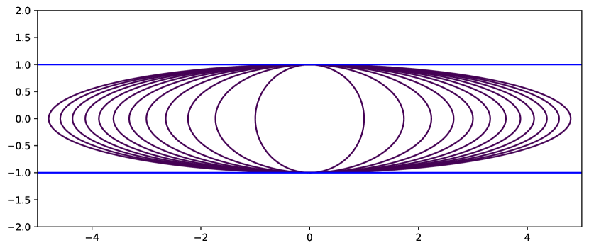
Figure 1: Ellipse converging to the two blue lines

We will show that if 3.7 holds true, then

(55) $$g(t):=\inf_{u\in E(t)}Q(t)u\cdot u$$

is right differentiable at $t=0^{+}$ by applying Theorem 2.12.

The Lagrangian $G:[0,\tau]\times{\mathbf{R}}^{d}\times{\mathbf{R}}\to{\mathbf{R}}$ associated with the minimisation problem (55) reads

(56) $$G(t,u,p):=Q(t)u\cdot u+p(A(t)u\cdot u-1).$$

By the Lagrangian multiplier rule we find for every minimiser $u^{t}\in X(t)$ a number $p^{t}\in{\mathbf{R}}$, such that

(57) $$Q(t)u^{t}+p^{t}A(t)u^{t}=0.$$

It also follows from (57) and $A(t)u^{t}\cdot u^{t}=1$, that

(58) $$g(t)=Q(t)u^{t}\cdot u^{t}=-p^{t}.$$

This shows that the set $Y(t,u^{t})=\{p^{t}\}$ is a singleton and also

(59) $$X(t)=\{u^{t}\in{\mathbf{R}}^{d}:\;Q(t)u^{t}+p^{t}(t)A(t)u^{t}=0,\quad A(t)u^{t}\cdot u^{t}=1\}.$$

The averaged adjoint equation associated with two states $(u^{0},u^{t})\in E(0)\times E(t)$ reads: find $q^{t}\in{\mathbf{R}}$ such that

(60) $$Q(t)(u^{t}+u^{0})+q^{t}A(t)(u^{t}+u^{0})=0.$$

The existence of $q^{t}$ can not be guaranteed for all pairs $(u^{0},u^{t})$; see Section 3.4 for a counter example. However, Theorem 2.12 only requires the existence of the averaged adjoint variable for certain pairs of states.

Remark 3.9.

We note that if 3.1, (b) is satisfied we have

(61) $$g(t)=\inf_{u\in E(t)}f(t,u)=\inf_{\begin{subarray}{c}u\in{\mathbf{R}}^{d}\\ u\neq 0\end{subarray}}\frac{Q(t)u\cdot u}{A(t)u\cdot u}.$$

Therefore in this case we can also apply Danskin’s theorem (see, e.g., [16, p. 524, Thm. 2.1], [9, p.140, Thm.5.1] or [4, Thm. 4.1]) to prove the right differentiability of $g$ at $t=0$ (in fact, one could even consider a more general $f(t,u)$ in this case). 3.1, (a) does not allow this simplification since $A$ is not necessarily positive definite in this case. Indeed consider the pair $(Q,A)$ from Example 3.6, (i) (which satisfies (a)):

(62) $$\inf_{\begin{subarray}{c}u\in{\mathbf{R}}^{2}\\ u\neq 0\end{subarray}}\frac{Qu\cdot u}{Au\cdot u}=\inf_{\begin{subarray}{c}u\in{\mathbf{R}}^{2}\\ u\neq 0\end{subarray}}\frac{x^{2}+y^{2}}{x^{2}-y^{2}}=-\infty,$$

while $\operatorname*{argmin}_{u\in E}x^{2}+y^{2}=\{(-1,0)^{\top},(1,0)^{\top}\}$ and hence $\min_{u\in E}Qu\cdot u=\min_{u\in E}x^{2}+y^{2}=1$ is finite.

3.3 Verification of the Hypotheses

We now verify Hypotheses (H0)–(H5) for the Lagrangian $G$ in (56) with $\tilde{X}=X={\mathbf{R}}^{d}$ and $Y={\mathbf{R}}$ and a real number $\tau>0$ which has to be chosen sufficiently small. In view of 3.1 it is clear that Hypothesis (H0) is satisfied. Hypotheses (H1) and (H2) are also obvious since $A$ and $Q$ are differentiable.

Verification of Hypothesis (H3)

To this end, we first prove the following lemma.

Lemma 3.10.

• For sufficiently small $\tau$ the set $S_{\tau}:=\cup_{t\in[0,\tau]}X(t)$ is bounded.

• For every null-sequence $(t_{n})$ and $u^{t_{n}}\in X(t_{n})$, there is a subsequence still indexed the same, and $u^{0}\in X(0)$, such that $u^{t_{n}}\to u^{0}$ as $n\to\infty$.

Proof 3.11.

We first show the boundedness of $S_{\tau}$ for $\tau$ small if either (a) or (b) of 3.1 hold. First suppose that 3.1, (a) is satisfied. Notice that $Q(t)$ is uniformly positive definite for all small $t$. Then by definition of $u^{t}\in X(t)$, we have for all $t\in[0,\tau]$,

(63) $$\alpha\|u^{t}\|^{2}\leq Q(t)u^{t}\cdot u^{t}\leq Q(t)u\cdot u\quad\text{ for all }u\in{\mathbf{R}}^{d},\;A(t)u\cdot u=1$$

for some $\alpha>0$. Now pick any $u^{0}\in{\mathbf{R}}^{d}$ with $A(0)u^{0}\cdot u^{0}=1$. By continuity we find $\tau>0$ and $c>0$ such that $A(t)u^{0}\cdot u^{0}\geq c>0$ for all $t\in[0,\tau]$ and hence $\hat{u}^{t}:=u^{0}/\sqrt{A(t)u^{0}\cdot u^{0}}$ satisfies $A(t)\hat{u}^{t}\cdot\hat{u}^{t}=1$ and thus $\hat{u}^{t}\in E(t)$. Then plugging $\hat{u}^{t}$ into (63) we obtain

(64) $$\alpha\|u^{t}\|^{2}\leq\frac{Q(t)u^{0}\cdot u^{0}}{A(t)u^{0}\cdot u^{0}}\leq c^{-1}\max_{t\in[0,\tau]}\|Q(t)\|\|u^{0}\|^{2}.$$

Thus $S_{\tau}$ is bounded.

Now suppose that 3.1, (b) holds. Since $A(0)$ is positive definite and since $A(\cdot)$ is continuous also $A(t)$ is positive definite provided $t$ is small enough. So we find $\alpha>0$, such that $\alpha\|u\|^{2}\leq A(t)u\cdot u$ for all $u\in{\mathbf{R}}^{d}$ and all small $t$. Therefore for all $u^{t}\in E(t)$ we have $\alpha\|u^{t}\|^{2}\leq A(t)u^{t}\cdot u^{t}=1$ which implies that $S_{\tau}$ is bounded.

The proof of $(ii)$ follows by standard arguments and hence is omitted.

Lemma 3.12.

For every null-sequence $(t_{n})$, we find $u^{0}\in X(0)$ and $p^{0}\in Y(0,u_{0})$, and a subsequence (denoted the same), elements $(u_{t_{n}}^{0},u^{t_{n}})\in E(0)\times X(t_{n})$ and $q^{t_{n}}\in Y(t_{n},u_{t_{n}}^{0},u^{t_{n}})$, such that

(65) $$q^{t_{n}}\to p^{0}\quad \text{ as }n\to\infty,$$

(66) $$u^{0}_{t_{n}}\to u^{0}\quad \text{ as }n\to\infty.$$

Proof 3.13.

Let $(t_{n})$ be an arbitrary null-sequence and let $(u^{t_{n}})$, $u^{t_{n}}\in X(t_{n})$ be given. Thanks to the previous Lemma 3.10 we find $u^{0}\in X(0)$ and a subsequence of $(t_{n})$, still indexed the same, such that $u^{t_{n}}\to u^{0}$ as $n\to\infty$. By the Lagrange multiplier rule we find $p^{0}\in Y(0,u^{0})$, such that

(67) $$Q(0)u^{0}+p^{0}A(0)u^{0}=0,\quad A(0)u^{0}\cdot u^{0}=1.$$

Since $A(0)u^{0}\cdot u^{0}=1$, we have $A(0)u^{t_{n}}\cdot u^{t_{n}}>0$ for $n$ large enough; therefore

(68) $$u^{0}_{t_{n}}:=\frac{1}{\sqrt{A(0)u^{t_{n}}\cdot u^{t_{n}}}}u^{t_{n}}\in E(0),$$

is well-defined. It is clear that $u^{0}_{t_{n}}\to u^{0}$ as $n\to\infty$. By construction $u^{0}_{t_{n}}$ and $u^{t_{n}}$ are linearly dependent. Since $u^{t_{n}}\in X(t_{n})$ the Lagrange multiplier rule shows $Q(t_{n})u^{t_{n}}+q^{t_{n}}A(t_{n})u^{t_{n}}=0$ for some $q^{t_{n}}\in{\mathbf{R}}$, and thus also

(69) $$Q(t_{n})(u^{0}_{t_{n}}+u^{t_{n}})+q^{t_{n}}A(t_{n})(u^{0}_{t_{n}}+u^{t_{n}})=0,$$

which is the averaged adjoint equation (60) associated with the pair $(u^{0}_{t_{n}},u^{t_{n}})$. Since $A(t_{n})(u^{0}_{t_{n}}+u^{t_{n}})\neq 0$ for $n$ large, it follows from (69) that

(70) $$q^{t_{n}}=-\frac{Q(t_{n})(u^{t_{n}}+u^{0}_{t_{n}})\cdot(u^{t_{n}}+u^{0}_{t_{n}})}{A(t_{n})(u^{t_{n}}+u^{0}_{t_{n}})\cdot(u^{t_{n}}+u^{0}_{t_{n}})}\to-\frac{Q(0)u^{0}\cdot u^{0}}{A(0)u^{0}\cdot u^{0}}=p^{0}.$$

This shows Hypothesis (H3) and finishes the proof.

Verification of Hypothesis (H4)

The verification of Hypothesis (H4) is a simple application of the inverse function theorem.

Lemma 3.14.

For every $u^{0}\in E(0)$ we find a differentiable function $t\mapsto u^{t}:[0,\tau]\to{\mathbf{R}}^{d}$ with $u^{t}\in E(t)$ for all $t\in(0,\tau]$.

Proof 3.15.

We argue similarly as in Lemma 3.12. Let $u^{0}\in{\mathbf{R}}^{d}$ with $A(0)u^{0}\cdot u^{0}=1$ be given. Again by continuity we find $\tau>0$ and $c>0$, such that $A(t)u^{0}\cdot u^{0}\geq c$ for all $t\in[0,\tau]$. Now

(71) $$u^{t}:=\frac{1}{\sqrt{A(t)u^{0}\cdot u^{0}}}$$

belongs to $E(t)$ and is right differentiable at $t=0$.

Verification of Hypothesis (H5)

To check Hypothesis (H5) we compute for all $u\in{\mathbf{R}}^{d}$ and $q\in{\mathbf{R}}$,

(72) $$\partial_{u}G(0,u,p)=(Q(0)+pA(0))u.$$

Hence by the fundamental theorem of calculus and (72) we obtain for all $u^{0}\in X(0)$, $u\in{\mathbf{R}}^{d}$ and $p^{0}\in Y(0,u^{0})$,

(73) $$\begin{split}|G(0,u,p^{0})-G(0,u^{0},p^{0})&-\partial_{u}G(0,u^{0},p^{0})(u-u^{0})|\\ &=|\int_{0}^{1}\partial_{u}G(0,su+(1-s)u^{0},p^{0})(u-u^{0})-\partial_{u}G(0,u^{0},p^{0})(u-u^{0})\;ds|\\ &\leq|u-u^{0}|^{2}2\|Q(0)+p^{0}A(0)\|\end{split}$$

and this verifies Hypothesis (H5).

Application of Theorem 2.12

Now we have verified all the Hypotheses of Theorem 2.12 and we obtain the following theorem.

Theorem 3.16.

Let $Q,A:[0,\tau]\to{\mathbf{R}}^{d\times d}$ be two continuously differentiable functions satisfying 3.7. Then the function $g$ is right differentiable at $t=0$ and we find $u^{0}\in X(0)$, such that

(74) $$dg(0)=\inf_{u\in X(0)}(Q^{\prime}(0)+p^{0}A^{\prime}(0))u\cdot u=(Q^{\prime}(0)+p^{0}A^{\prime}(0))u^{0}\cdot u^{0},$$

where $(u^{0},p^{0})\in{\mathbf{R}}^{d}\times{\mathbf{R}}$ satisfies:

$$Q(0)u^{0}+p^{0}A(0)u^{0} =0,\qquad p^{0}=-Q(0)u^{0}\cdot u^{0},$$

$$A(0)u^{0}\cdot u^{0} =1.$$

We can even obtain more using the differentiability of the suboptimal paths $u^{t}$ of Lemma 3.14 and the arguments of Lemma 2.15. In contrast to the previous theorem the following lemma holds for all elements $u^{0}\in X(0)$.

Lemma 3.17.

Let $u^{0}\in X(0)$. Let $v\in{\mathbf{R}}^{d}$ be any vector, such that there is $(u^{t})$ with $u^{t}\in E(t)$ satisfying

(75) $$v=\lim_{t\searrow 0}\frac{u^{t}-u^{0}}{t}\quad\text{ and }\quad A^{\prime}(0)u^{0}\cdot u^{0}\neq 0.$$

Then we have

(76) $$dg(0)\leq\partial_{t}G(0,u^{0},\mu)=(Q^{\prime}(0)+\mu A^{\prime}(0))u^{0}\cdot u^{0},$$

where $\mu$ is given by

(77) $$\mu:=-\frac{Q(0)u^{0}\cdot v}{A(0)u^{0}\cdot v}.$$

Proof 3.18.

Let $u^{0}\in X(0)$ and let $u^{t}$ be a differentiable path with $v:=\lim_{t\searrow 0}(u^{t}-u^{0})/t$. By definition $A(t)u^{t}\cdot u^{t}=1$ and hence $A^{\prime}(0)u^{0}\cdot u^{0}+2A(0)u^{0}\cdot v=0$. In view of $A^{\prime}(0)u^{0}\cdot u^{0}\neq 0$, we conclude

(78) $$A(0)u^{0}\cdot v\neq 0.$$

Now we choose $q^{t}\in{\mathbf{R}}$ such that

(79) $$\begin{split}\int_{0}^{1}&\partial_{u}G(t,su^{t}+(1-s)u^{0},q^{t})(u^{t}-u^{0})\\ &=2(Q(t)+q^{t}A(t))(u^{t}-u^{0})=0.\end{split}$$

It is readily checked using (78) that $A(t)(u^{t}+u^{0})\cdot(\frac{u^{t}-u^{0}}{t})\neq 0$ for all $t$ small and thus we obtain from (79),

(80) $$\begin{split}q^{t}&=-\frac{Q(t)(u^{t}+u^{0})\cdot(\frac{u^{t}-u^{0}}{t})}{A(t)(u^{t}+u^{0})\cdot(\frac{u^{t}-u^{0}}{t})}\to-\frac{Q(0)u^{0}\cdot v}{A(0)u^{0}\cdot v}=:\mu.\end{split}$$

Now we apply the mean value theorem to obtain

(81) $$G(t,u^{t},q^{t})-G(t,u^{0},q^{t})=\int_{0}^{1}\partial_{u}G(t,su^{t}+(1-s)u^{0},q^{t})(u^{t}-u^{0})\;ds=0,$$

where the last equality follows from the definition of $q^{t}$. Hence we obtain that for every null-sequence $t\searrow 0$ and every $u^{0}\in X(0)$, we find $u^{t}\in E(t)$ and $q^{t}\in{\mathbf{R}}$, such that

(82) $$G(t,u^{t},q^{t})=G(t,u^{0},q^{t}).$$

Hence we can use the same arguments as in Lemma 2.15 to conclude $dg(0)\geq\partial_{t}G(0,u^{0},\mu)$.

3.4 On the condition (H3) and non-existence of averaged adjoints

Let us give an explicit example where for all sufficiently small $t>0$ and any pair $(u^{0},u^{t})\in X(0)\times X(t)$ the set of averaged adjoints $Y(t,u^{0},u^{t})=\emptyset$ is empty. However, for every $u^{t}\in X(t)$, we find $u^{0}\in X(0)$ and $u^{t}_{0}\in E(0)$, such that $u^{t}_{0}\to u^{0}$ and $Y(t,u^{t}_{0},u^{t})\neq\emptyset$. Therefore Hypothesis (H3) is necessary in some cases and can not be simplified.

Consider again $g$ defined by (55) with

(83) $$E(t) =\{u=(x,y)^{\top}\in{\mathbf{R}}^{2}:\;A(t)u\cdot u=1\},$$

(84) $$A(t) :=\begin{pmatrix}1&t\\ t&1\end{pmatrix},\qquad Q=\begin{pmatrix}1&0\\ 0&2\end{pmatrix}.$$

Clearly 3.7 is satisfied for this example and hence $g$ is right differentiable thanks to Theorem 3.16. At $t=0$ we have

(85) $$E(0)=\{(x,y)^{\top}\in{\mathbf{R}}^{2}:\;x^{2}+y^{2}=1\},\quad X(0)=\{(\pm 1,0)^{\top}\},\quad Y(0,(\pm 1,0)^{\top})=\{1\}$$

and for $t>0$ and $u^{t}\in X(t)$ we find $p^{t}\in Y(t,u^{t})$ solving

(86) $$Qu^{t}+p^{t}A(t)u^{t}=0\quad\Leftrightarrow\quad A(t)^{-1}Qu^{t}+p^{t}u^{t}=0.$$

We compute

(87) $$A(t)^{-1}Q=\frac{1}{1-t^{2}}\underbrace{\begin{pmatrix}1&-2t\\ -t&2\end{pmatrix}}_{=:\tilde{A}(t)}.$$

The eigenvalues of $\tilde{A}(t)$ are given by

(88) $$\lambda^{\pm}(t)=\frac{1}{2}\left(3\pm\sqrt{1+8t^{2}}\right)$$

and therefore $\{\frac{1}{1-t^{2}}\lambda^{-}(t),\frac{1}{1-t^{2}}\lambda^{+}(t)\}$ are the eigenvalues of $A(t)^{-1}Q$ and the eigenspaces are one dimensional. Moreover, $g(t)=\frac{1}{1-t^{2}}\lambda^{-}(t)$. For small $t>0$ we have $\lambda^{+}(t)>2$ and $\lambda^{-}(t)<1$. The corresponding eigenvalue equations lead to

(89) $$x(\lambda^{\pm}-1) =-2ty,$$

(90) $$y(\lambda^{\pm}-2) =-tx.$$

So for $\lambda^{+}$ we obtain as eigenvector for $t>0$,

(91) $$u^{t}_{+}=\begin{pmatrix}a^{t}\\ 1\end{pmatrix},\quad a^{t}=\frac{-2t}{\lambda^{+}(t)-1}<0,$$

and $a^{t}\to 0$ for $t\searrow 0$. Similarly, for $\lambda^{-}$ we obtain

(92) $$u_{-}^{t}=\begin{pmatrix}1\\ b^{t}\end{pmatrix},\quad b^{t}=\frac{-t}{\lambda^{-}(t)-2}>0,$$

and $b^{t}\to 0$ for $t\searrow 0$. It follows that

(93) $$X(t)=\{\hat{u}_{-}^{t},-\hat{u}_{-}^{t}\},\quad\hat{u}_{-}^{t}:=\frac{1}{\sqrt{A(t)u_{-}^{t}\cdot u_{-}^{t}}}u_{-}^{t}.$$

Now let us check that the averaged adjoint equation is not solvable.

Lemma 3.19.

For $t>0$ small and for $(\hat{u}^{t}_{-},\pm u^{0})$ with $u^{0}=(1,0)^{\top}$, there is no $q^{t}\in{\mathbf{R}}$, such that

(94) $$Q(\hat{u}^{t}_{-}\pm u^{0})+q^{t}A(t)(\hat{u}^{t}_{-}\pm u^{0})=0.$$

In particular $Y(t,u^{0},u^{t}_{-})=Y(t,-u^{0},u^{t}_{-})=\emptyset$ and no averaged adjoint state for such pairs exists.

Proof 3.20.

Suppose $q^{t}\in Y(t,u^{0},u_{-}^{t})$ exists. Then in view of the definition (94), this means that $q^{t}\in\{-\frac{1}{1-t^{2}}\lambda^{-}(t),-\frac{1}{1-t^{2}}\lambda^{+}(t)\}$ and in view of (94)

(95) $$\begin{split}\hat{u}^{t}_{-}+u^{0}=&\frac{1}{\sqrt{A(t)u_{-}^{t}\cdot u_{-}^{t}}}\begin{pmatrix}1\\ b^{t}\end{pmatrix}+\begin{pmatrix}1\\ 0\end{pmatrix}\end{split}$$

must be an eigenvector of $A(t)^{-1}Q$. Since the eigenspaces are one dimensional, we must have one of the two cases:

(96a) $$\hat{u}^{t}_{-}+u^{0}=\alpha u^{t}_{-},$$

(96b) $$\hat{u}^{t}_{-}+u^{0}=\alpha u^{t}_{+},$$

for some $\alpha\in{\mathbf{R}}$. By comparing the last component of the vectors of (96a), we see that equality in (96a) can only happen for $\alpha=\frac{1}{\sqrt{A(t)u_{-}^{t}\cdot u_{-}^{t}}}$, which gives

(97) $$\hat{u}^{t}_{-}+u^{0}=\hat{u}_{-}^{t}\quad\Rightarrow\quad u^{0}=0$$

and thus a contradiction. Similarly for (96b), we compare the last component and see that equality can only be true for $\alpha=\frac{b^{t}}{\sqrt{A(t)u^{t}_{-}\cdot u^{t}_{-}}}$, which leads to

(98) $$\hat{u}^{t}_{-}+u^{0}=\frac{b^{t}}{\sqrt{A(t)u_{-}^{t}\cdot u_{-}^{t}}}\begin{pmatrix}a^{t}\\ 1\end{pmatrix}$$

which is also impossible since $a^{t}\to 0$ and $b^{t}\to 0$ and hence the right vector goes to zero as $t\searrow 0$, however, the left hand side goes to $2u^{0}\neq 0$. Therefore (94) is not solvable and $Y(t,u^{0},u^{t}_{-})=\emptyset$. The same arguments show that $Y(t,-u^{0},u^{t}_{-})=\emptyset$.

Despite this negative result, we can define for every $u^{t}\in X(t)$ the element $u^{0}_{t}:=u^{t}/\sqrt{A(0)u^{t}\cdot u^{t}}\in E(0)$, which is linearly dependent on $u^{t}$ and hence $Y(t,u^{0}_{t},u^{t})\neq\emptyset$. Moreover, if $u^{t}$ converges, also $u^{0}_{t}$ converges.

3.5 Second order sufficient conditions

Let us finish this section by making some remarks on second order analysis results. We notice that in [5, Sec. 4.9.1., p. 365] equality constraints are treated using second order analysis. However, for our problem this is not applicable. In fact in [5, Thm. 4.125, p. 365] the following problem is studied

(99) $$g(t)=\inf_{u\in E(t)}f(t,u),\quad E(t)=\{u^{t}\in X:\;e(t,u^{t})=0\},$$

where $f:[0,\tau]\times X\to{\mathbf{R}}$ and $e:[0,\tau]\times X\to Y$ are two times differentiable functions. Introduce the associated Lagrangian

(100) $$G(t,u,p):=f(t,u)+\langle p,e(t,u)\rangle_{Y^{*},Y},\quad t\in[0,\tau],\;u\in X,\;p\in Y^{*}.$$

Suppose that $\partial_{u}e(0,u^{0}):X\to Y$ is surjective, such that the Lagrange multiplier $q^{0}\in Y(0,u^{0})$ for every $u^{0}\in X(0)$ is unique. Then in [5, Thm. 4.125, p. 365] it is proved that for given $u^{0}\in X(0)$ and $q^{0}\in Y(0,u^{0})$, there exist locally unique solutions $(u^{t},p^{t})$ of

(101) $$\partial_{u}G(t,u^{t},p^{t})=\partial_{u}f(t,u^{t})+\langle p^{t},\partial_{u}e(t,u^{t})\rangle_{Y^{*},Y} =0,$$

(102) $$e(t,u^{t}) =0,$$

provided the second order condition holds:

(103) $$\exists\alpha>0,\;\partial_{u}^{2}G(0,u^{0},p^{0})(v)(v)\geq\alpha\|v\|^{2}_{X}\quad\text{ for all }v\in\text{kern}(\partial_{u}e(0,u^{0})).$$

This is a consequence of the implicit function theorem. However, this does not work in our setting in general since the second order condition for (53) reads with $X={\mathbf{R}}^{d}$ equipped with the Euclidean norm $\|\cdot\|$, $Y={\mathbf{R}}$, $e(t,u)=A(t)u\cdot u-1$ and $f(t,u):=Q(t)u\cdot u$:

(104) $$\exists\alpha>0,\;(Q(0)+p^{0}A(0))v\cdot v\geq\alpha\|v\|^{2}\quad\text{ for all }v\in(A(0)u^{0})^{\bot}.$$

Then (101) would read:

(105) $$(Q(t)+p^{t}A(t))u^{t}=0,\quad A(t)u^{t}\cdot u^{t}=1.$$

However, it is readily seen that (104) cannot hold when the eigenvalue $-p^{0}$ of $(Q(0),A(0))$ is not simple. Take for instance $A(0)=I$, $Q(0)=Q(0)^{\top}$, and assume $-p^{0}$ is not geometrically simple (i.e., the eigenspace has dimension $\geq 2$) eigenvalue of $Q(0)$. Then (104) cannot hold, since $\text{kern}(A(0)u^{0})=(u^{0})^{\bot}=\{v\in{\mathbf{R}}^{d}:v\cdot u^{0}=0\}$ contains another eigenvector $v\in(u^{0})^{\bot}$ associated with $-p^{0}$ and thus $Q(0)v\cdot v+p^{0}\|v\|^{2}=0$.

4 Application to a shape optimisation problem

In this section we present another example where Theorem 2.12 is applicable. In contrast to the previous section this example is infinite dimensional.

4.1 Shape optimisation problem

For every bounded Lipschitz domain $\Omega\subset{\mathbf{R}}^{d}$, $d\in\{2,3\}$, we consider

(106) $$J(\Omega):=\inf_{u\in E(\Omega)}f(\Omega,u),$$

where

(107) $$f(\Omega,u):=\int_{\Omega}|u-u_{r}|^{2}\;dx+\gamma\int_{\Omega}|\nabla u|^{2}\;dx,\quad\gamma>0,\;u_{r}\in H^{1}({\mathbf{R}}^{d}),$$

and $E(\Omega)$ comprises the set of solutions $u=u_{\Omega}\in H^{1}(\Omega)$ to the semilinear problem:

(108) $$\int_{\Omega}\nabla u\cdot\nabla\varphi+\varrho(u)\varphi\;dx=\int_{\Omega}f\varphi\;dx$$

for all $\varphi\in H^{1}_{0}(\Omega)$. We make the following assumption.

Assumption 4.1.

We assume that $\varrho:{\mathbf{R}}\to{\mathbf{R}}$ is a two times differentiable, Lipschitz continuous and strongly monotone function satisfying $\varrho(0)=0$. We also assume $f\in H^{1}({\mathbf{R}}^{d})$.

Equation (108) cannot be uniquely solvable since no Dirichlet boundary conditions are prescribed. Given a function $u_{r}$ the cost $J(\Omega)$ measures the best solution to (108) which is closest to $u_{r}$. The set $E(\Omega)$ contains infinitely many elements and is nonconvex (unless $\varrho$ is linear).

Lemma 4.2.

There exists a minimiser to the problem (106).

Proof 4.3.

It is clear that $J(\Omega)$ is finite. Let $(u_{n})$ be a minimising sequence in $H^{1}(\Omega)$, so that

(109) $$J(\Omega)=\lim_{n\to\infty}\left(\int_{\Omega}|u_{n}-u_{r}|^{2}\;dx+\gamma\int_{\Omega}|\nabla u_{n}|^{2}\;dx\right).$$

From this it immediately follows that $(u_{n})$ is bounded in $H^{1}(\Omega)$. Hence due to Rellich’s compactness theorem we find $u\in H^{1}(\Omega)$ and a subsequence, which is denoted the same, such that $\nabla u_{n}\rightharpoonup\nabla u$ weakly in $L_{2}(\Omega)^{d}$ and $u_{n}\to u$ strongly in $L_{2}(\Omega)$. Hence we can pass to the limit $n\to\infty$ in

(110) $$\int_{\Omega}\nabla u_{n}\cdot\nabla\varphi+\varrho(u_{n})\varphi\;dx=\int_{\Omega}f\varphi\;dx\quad\text{ for all }\varphi\in H^{1}_{0}(\Omega)$$

to conclude $u\in E(\Omega)$. In addition we infer from (109)

(111) $$\int_{\Omega}|u-u_{r}|^{2}\;dx+\gamma\int_{\Omega}|\nabla u|^{2}\;dx\leq J(\Omega).$$

This shows that $u$ is a minimiser and finishes the proof.

Our goal is now to use Theorem 2.12 to show that the directional shape derivative of $J$ exists.

Definition 4.4.

The directional shape derivative of $J$ at $\Omega$ in direction $X\in C^{0,1}({\mathbf{R}}^{d})^{d}$ is defined by

(112) $$dJ(\Omega)(X):=\lim_{t\searrow 0}\frac{J((\mathsf{Id}+tX)(\Omega))-J(\Omega)}{t}.$$

Notice that the mapping $T_{t}:=\text{id}+tX:{\mathbf{R}}^{d}\to{\mathbf{R}}^{d}$ is a bi-Lipschitz mapping for all $|t|<1/L(X)$, where $L(X)$ denotes the Lipschitz constant of $X$.

Let us introduce the Lagrangian $G:H^{1}(\Omega)\times H^{1}_{0}(\Omega)\to{\mathbf{R}}$ by

(113) $$G(\varphi,\psi):=\int_{\Omega}|\varphi-u_{r}|^{2}\;dx+\gamma\int_{\Omega}|\nabla\varphi|^{2}\;dx+\int_{\Omega}\nabla\varphi\cdot\nabla\psi+\varrho(\varphi)\psi\;dx-\int_{\Omega}f\psi\;dx.$$

Lemma 4.2 guarantees that the set

(114) $$X(\Omega):=\{u\in E(\Omega):\inf_{\varphi\in E(\Omega)}G(\varphi,0)=G(u,0)\}$$

is not empty. In the next paragraph we consider the perturbed versions of $E(\Omega)$ and $X(\Omega)$.

4.2 Analysis of the perturbed problems

We will show by applying Theorem 2.12 that for a bounded Lipschitz domain $\Omega\subset{\mathbf{R}}^{d}$ the directional shape derivative of $J$ exists. At first we consider any solution $u_{t}\in H^{1}(\Omega_{t})$ defined on the perturbed domain $\Omega_{t}:=T_{t}(\Omega)$ of

(115) $$\int_{\Omega_{t}}\nabla u_{t}\cdot\nabla\varphi+\varrho(u)\varphi\;dx=\int_{\Omega_{t}}f\varphi\;dx\quad\text{ for all }\varphi\in H^{1}_{0}(\Omega_{t}).$$

Now since $\varphi\in H^{1}(T_{t}(\Omega))$ (resp. $\varphi\in H^{1}_{0}(T_{t}(\Omega))$) if and only if $\varphi\circ T_{t}\in H^{1}(\Omega)$ (resp. $\varphi\circ T_{t}\in H^{1}_{0}(\Omega)$) (see [37, Thm. 2.2.2, p.52]) changing variables in (115) shows that $u^{t}:=u_{t}\circ T_{t}\in H^{1}(\Omega)$ solves

(116) $$\int_{\Omega}A(t)\nabla u^{t}\cdot\nabla\varphi+|\det(\partial T_{t})|\varrho(u^{t})\varphi\;dx=\int_{\Omega}f^{t}\varphi\;dx\quad\text{ for all }\varphi\in H^{1}_{0}(\Omega),$$

where

(117) $$A(t):=\det(\partial T_{t})\partial T_{t}^{-1}\partial T_{t}^{-\top},\quad f^{t}:=\det(\partial T_{t})f\circ T_{t}.$$

Therefore $u_{t}\in E(T_{t}(\Omega))$ if and only if $u^{t}:=u_{t}\circ T_{t}$ is in

(118) $$E(t):=\left\{u^{t}\in H^{1}(\Omega):\;u^{t}\text{ solves }\eqref{eq:state_ut_}\right\}.$$

As a result we get for $t$ small

(119) $$g(t):=J(T_{t}(\Omega))=\inf_{u\in E(t)}f(t,u),$$

where

(120) $$f(t,u):=\int_{\Omega}\det(\partial T_{t})(u-u_{r}^{t})^{2}\;dx+\gamma\int_{\Omega}A(t)\nabla u^{t}\cdot\nabla u^{t}\;dx,$$

where $u_{r}^{t}:=u_{r}\circ T_{t}$. This problem falls into the framework of Theorem 2.12.

We recall the following proposition; see, e.g., [34].

Proposition 4.5.

Let $\mathsf{D}\subset{\mathbf{R}}^{d}$ be a bounded and open set. Let $X:{\mathbf{R}}^{d}\to{\mathbf{R}}^{d}$ be a Lipschitz vector field. Then for $T_{t}:=id+tX$ there holds:

• We have

  $$\frac{\partial T_{t}-I}{t}\rightarrow \partial X \text{ strongly in }C(\overline{\mathsf{D}},{\mathbf{R}}^{d,d})$$

  $$\frac{\partial T_{t}^{-1}-I}{t}\rightarrow -\partial X \text{ strongly in }C(\overline{\mathsf{D}},{\mathbf{R}}^{d,d})$$

  $$\frac{\det(\partial T_{t})-1}{t}\rightarrow \operatorname{div}(X) \text{ strongly in }C(\overline{\mathsf{D}}).$$

• For all open sets $\Omega\subset\mathsf{D}$ and all $\varphi\in H^{1}({\mathbf{R}}^{d})$, we have

  (121) $$\frac{\varphi\circ T_{t}-\varphi}{t}\rightarrow \nabla\varphi\cdot X \text{ strongly in }L_{2}(\Omega).$$

Lemma 4.6.

Let $u^{0}\in E(0)$ be given. Then we find a path $t\mapsto u^{t}:[0,\tau]\rightarrow H^{1}(\Omega)$ with $u^{t}\in E(t)$, $u^{t}-u^{0}\in H^{1}_{0}(\Omega)$, and a constant $c$, such that

(122) $$\|u^{t}-u^{0}\|_{H^{1}}\leq ct\quad\text{ for all }t\in[0,\tau].$$

Proof 4.7.

Let $u^{0}\in E(0)$ be given. By definition $u^{0}\in H^{1}(\Omega)$ solves:

(123) $$\int_{\Omega}\nabla u^{0}\cdot\nabla\varphi+\varrho(u^{0})\varphi\;dx=\int_{\Omega}f\varphi\;dx\quad\text{ for all }\varphi\in H^{1}_{0}(\Omega).$$

Set $g_{0}:=u^{0}|_{\partial\Omega}$ and consider for every $t\in[0,\tau]$: find $u^{t}\in H^{1}(\Omega)$, such that $u^{t}=g_{0}$ on $\partial\Omega$ and

(124) $$\int_{\Omega}A(t)\nabla u^{t}\cdot\nabla\varphi+\operatorname{det}(\partial T_{t})\varrho(u^{t})\varphi\;dx=\int_{\Omega}f^{t}\varphi\;dx\quad\text{ for all }\varphi\in H^{1}_{0}(\Omega).$$

By construction $u^{t}$ is uniquely determined, $u^{t}\in E(t)$, $u^{t}-u^{0}=0$ on $\partial\Omega$ for all $t$. We obtain from (124):

(125) $$\int_{\Omega}A(t) \nabla(u^{t}-u^{0})\cdot\nabla\varphi\;dx+\int_{\Omega}\operatorname{det}(\partial T_{t})(\varrho(u^{t})-\varrho(u^{0}))\varphi\;dx$$

$$= -\int_{\Omega}\operatorname{det}(\partial T_{t})\varrho(u^{0})\varphi-f^{t}\varphi+A(t)\nabla u^{0}\cdot\nabla\varphi\;dx$$

$$= -\int_{\Omega}(\operatorname{det}(\partial T_{t})-1)\varrho(u^{0})\varphi-(f^{t}-f)\varphi+(A(t)-I)\nabla u^{0}\cdot\nabla\varphi\;dx$$

for all $\varphi\in H^{1}_{0}(\Omega)$. Since $\varphi:=u^{t}-u^{0}$ is zero on $\partial\Omega$ we may use it as test function in (125). Hence using Hölder’s inequality, the uniform monotonicity of $A$ and the monotonicity $(\varrho(x)-\varrho(y))(x-y)\geq 0$ for all $x,y\in{\mathbf{R}}$ gives

(126) $$\int_{\Omega} (u^{t}-u^{0})^{2}+|\nabla(u^{t}-u^{0})|^{2}\;dx$$

$$\leq c(\|f^{t}-f\|_{C(\overline{\Omega})}+\|A(t)-I\|_{C(\overline{\Omega})^{d\times d}}\|u^{0}\|_{H^{1}(\Omega)}+\|\operatorname{det}(\partial T_{t})-1\|_{C(\overline{\Omega})}\|\varrho(u_{0})\|_{C(\mkern 1.5mu\overline{\mkern-1.5mu\Omega\mkern-1.5mu}\mkern 1.5mu)})$$

and therefore it follows from Proposition 4.5,

(127) $$\|u^{t}-u^{0}\|_{H^{1}(\Omega)}\leq ct\quad\text{ for all }t\in[0,\tau].$$

Parametrised Lagrangian and averaged adjoint

We set $\tilde{X}=Y:=H^{1}_{0}(\Omega)$ and $X:=H^{1}(\Omega)$. The parametrised Lagrangian $G:[0,\tau]\times X\times Y\rightarrow{\mathbf{R}}$ is given by

(128) $$G(t,u,p)= \int_{\Omega}\det(\partial T_{t})(u-u_{r}^{t})^{2}\;dx+\gamma\int_{\Omega}A(t)\nabla u\cdot\nabla u\;dx$$

$$+\int_{\Omega}A(t)\nabla u\cdot\nabla p+\operatorname{det}(\partial T_{t})\varrho(u)p-f^{t}p\;dx,$$

where we recall $A(t)=\operatorname{det}(\partial T_{t})\partial X^{-1}\partial X^{-\top}$, $u_{r}^{t}=u_{r}\circ T_{t}$ and $f^{t}=\operatorname{det}(\partial T_{t})f\circ T_{t}$. It is noteworthy that in this example we have $\tilde{X}\neq X$. Using Proposition 4.5 we see that $A(t)$ and $f^{t}$ are differentiable and we readily check for all $u,p\in H^{1}(\Omega)$:

(129) $$\partial_{t}G(0,u,p)= \int_{\Omega}\operatorname{div}(X)(u-u_{r})^{2}-(u-u_{r})\nabla u_{r}\cdot X+\gamma A^{\prime}(0)\nabla u\cdot\nabla u\;dx$$

$$+\int_{\Omega}A^{\prime}(0)\nabla u\cdot\nabla p+\operatorname{div}(X)\varrho(u)p-f^{\prime}p\;dx,$$

where $A^{\prime}(0)=\operatorname{div}(X)I-\partial X-\partial X^{\top}$ and $f^{\prime}=\operatorname{div}(X)f+\nabla f\cdot X$. It is also readily checked that assumptions (H0)–(H3) are satisfied. Moreover, since $\varrho$ is Lipschitz continuous we also readily check Hypothesis (H5).

The averaged adjoint associated with $u^{t}\in E(t)$ and $u^{0}\in E(0)$ reads: find $q^{t}\in H^{1}_{0}(\Omega)$, such that,

(130) $$\int_{\Omega}A(t)\nabla q^{t} \cdot\nabla\varphi+\int_{0}^{1}\operatorname{det}(\partial T_{t})\varrho^{\prime}(su^{t}+(1-s)u^{0})q^{t}\;ds\varphi\;dx$$

$$=-\int_{\Omega}\operatorname{det}(\partial T_{t})(2u_{r}^{t}-(u^{t}+u^{0}))\varphi\;dx-\int_{\Omega}\operatorname{det}(\partial T_{t})A(t)\nabla(u^{t}+u^{0})\cdot\nabla\varphi\;dx$$

for all $\varphi\in H^{1}_{0}(\Omega)$. It follows from the theorem of Lax-Milgram and the uniform coercivity of $A$ and $\operatorname{det}(\partial T_{t})$ that (130) admits a unique solution.

Lemma 4.8.

For every null-sequence $(t_{n})$ and $(u^{t_{n}})$, $u^{t_{n}}\in X(t_{n})$ there is a subsequence $(t_{n_{k}})$ and $u^{0}\in X(0)$, such that

(131) $$u^{t_{n_{k}}}\rightharpoonup u^{0}\quad\text{ in }H^{1}(\Omega)\quad\text{ as }k\rightarrow\infty.$$

Proof 4.9.

Let $(t_{n})$ be a null-sequence and $u^{t_{n}}\in X(t_{n})$. By definition we have for all $n\geq 1$

(132) $$J(T_{t_{n}}(\Omega))\leq\int_{\Omega}\det(\partial T_{t_{n}})(u-u_{r}^{t_{n}})^{2}\;dx+\gamma\int_{\Omega}A(t_{n})\nabla u\cdot\nabla u\;dx\quad\text{ for all }u\in E(t_{n}).$$

Now fix $u^{0}\in E(0)$ and let $(\bar{u}^{t})\in E(t)$ be as in Lemma 4.6, such that $\bar{u}^{t}\to u^{0}$ in $H^{1}(\Omega)$. Plugging $\bar{u}^{t_{n}}$ into (132) and using Proposition 4.5, we find $C>0$, such that

(133) $$J(T_{t_{n}}(\Omega))\leq C\quad\text{ for all }n\geq 1.$$

It follows in particular, since

(134) $$J(T_{t_{n}}(\Omega))=\int_{\Omega}\det(\partial T_{t_{n}})(u^{t_{n}}-u_{r}^{t_{n}})^{2}\;dx+\gamma\int_{\Omega}A(t_{n})\nabla u^{t_{n}}\cdot\nabla u^{t_{n}}\;dx,$$

that $(u^{t_{n}})$ is bounded. Hence there is a subsequence (denoted the same) and $u^{0}\in H^{1}(\Omega)$, such that $u^{t_{n}}\rightharpoonup u^{0}$ weakly in $H^{1}(\Omega)$ and $u^{t_{n}}\to u^{0}$ strongly in $L_{2}(\Omega)$. It is readily checked that by passing to the limit $n\to\infty$ that $u^{0}\in X(0)$, which finishes the proof.

Corollary 4.10.

For every null-sequence $(t_{n})$ and $u^{t_{n}}\in X(t_{n})$, we find $u^{0}\in X(0)$ and $p^{0}\in Y(0,u^{0})$, and a subsequence (denoted the same), elements $(u^{t_{n}}_{0},u^{t_{n}})\in E(0)\times X(t_{n})$ and $q^{t_{n}}\in Y(t,u_{0}^{t_{n}},u^{t_{n}})$, such that $u^{t_{n}}-u^{0,t_{n}}\in H^{1}_{0}(\Omega)$ and

(135) $$u^{0}_{t_{n}}\rightharpoonup u^{0} \quad\text{ in }H^{1}(\Omega)\quad\text{ as }n\rightarrow\infty,$$

(136) $$q^{0}_{t_{n}}\rightharpoonup q^{0} \quad\text{ in }H^{1}_{0}(\Omega)\quad\text{ as }n\rightarrow\infty.$$

Proof 4.11.

Thanks to Lemma 4.8 we find for every null-sequence $(t_{n})$ and $u^{t_{n}}\in X(t_{n})$ a subsequence (denoted the same) and $u^{0}\in X(0)$, such that $u^{t_{n}}\rightharpoonup u^{0}$ weakly in $H^{1}(\Omega)$. Set $g_{n}:=u^{t_{n}}|_{\partial\Omega}$ and consider: find $u^{0}_{t_{n}}\in H^{1}(\Omega)$ with $u^{0}_{t_{n}}=g_{n}$ on $\partial\Omega$, such that

(137) $$\int_{\Omega}\nabla u^{0}_{t_{n}}\cdot\nabla\varphi+\varrho(u^{0}_{t_{n}})\varphi\;dx=\int_{\Omega}f\varphi\;dx\quad\text{ for all }\varphi\in H^{1}_{0}(\Omega).$$

By construction $u^{0}_{t_{n}}$ is uniquely determined and $u^{0}_{t_{n}}\in E(0)$. If we introduce $\tilde{u}_{n}:=u^{t_{n}}-u^{0}_{t_{n}}$, then $\tilde{u}_{n}\in H^{1}_{0}(\Omega)$ and

(138) $$\int_{\Omega} \nabla\tilde{u}_{n}\cdot\nabla\varphi+(\varrho(u^{t_{n}})-\varrho(u^{0}_{t_{n}}))\varphi\;dx$$

$$=\int_{\Omega}(I-A(t_{n}))\nabla u^{t_{n}}\cdot\nabla\varphi+(1-\operatorname{det}(\partial T_{t}))\varrho(u^{t_{n}})\varphi+(f^{t}-f)\varphi\;dx$$

for all $\varphi\in H^{1}_{0}(\Omega)$. So testing (138) with $\varphi=\tilde{u}_{n}$ and using Hölder’s inequality yields

(139) $$\|\tilde{u}_{n}\|_{H^{1}}\leq c(\|A(t_{n})-I\|_{C(\mkern 1.5mu\overline{\mkern-1.5mu\Omega\mkern-1.5mu}\mkern 1.5mu,{\mathbf{R}}^{d,d})}+\|1-\operatorname{det}(\partial T_{t})\|_{C(\overline{\Omega})}\|u^{t_{n}}\|_{H^{1}(\Omega)}+\|f^{t}-f\|_{L_{2}})\|u^{t_{n}}\|_{H^{1}}$$

and since $(u^{t_{n}})$ is bounded in $H^{1}(\Omega)$ the result follows from Proposition 4.5. It follows that $u^{t_{n}}-u^{0,t_{n}}\rightharpoonup 0$ in $H^{1}(\Omega)$ and since $u^{t_{n}}\rightharpoonup u^{0}$ in $H^{1}(\Omega)$ we also conclude that $u^{0,t_{n}}$ converges weakly to $u^{0}$ in $H^{1}(\Omega)$. From this and (130) it is also readily seen that the averaged adjoint $q^{t_{n}}$ for $(u^{t_{n}}_{0},u^{t_{n}})$ exists and that $q^{t_{n}}\rightharpoonup q^{0}$ weakly in $H^{1}(\Omega)$ as $n\to\infty$.

Application of Theorem 2.12

We have verified that assumptions (H0)–(H5) of Theorem 2.12 are satisfied for $G$ defined in (128) with $Y=\tilde{X}=H^{1}_{0}(\Omega)$ and $X=H^{1}(\Omega)$. Therefore we obtain the following theorem.

Theorem 4.12.

The right derivative of $g$ at $t=0^{+}$ exists and

(140) $$dg(0)=\inf_{u\in X(0)}\partial_{t}G(0,u,p^{0}(u)),$$

where $p^{0}(u)\in H^{1}_{0}(\Omega)$ solves

(141) $$\int_{\Omega}\nabla p^{0}(u)\cdot\nabla\varphi+\varrho^{\prime}(u)p^{0}(u)\varphi\;dx=-\int_{\Omega}2(u-u_{r})\varphi+2\gamma\nabla u\cdot\nabla\varphi\;dx$$

for all $\varphi\in H^{1}_{0}(\Omega)$ and $\partial_{t}G(0,u,p^{0}(u))$ is given by (129).

Conclusion

In this paper we discussed a new minimax theorem and presented two examples. In both examples we could establish right differentiability of the corresponding value function.

In a future work it would be interesting to apply our result to optimal control problems with non-unique solution. Also to find an example where for the state $u^{0}\in X(0)$ the adjoint $Y(0,u^{0})$ is not a singleton is still an open question.

References

- [1] H.Amann and J.Escher, Analysis. II, Birkhäuser Verlag, Basel, 2008. Translated from the 1999 German original by Silvio Levy and Matthew Cargo.
- [2] J. F.Bonnans and R.Cominetti, Perturbed optimization in Banach spaces I: a general theory based on a weak directional constraint qualification, SIAM Journal on Control and Optimization 34 (1996), 1151–1171, doi:10.1137/s0363012994267273.
- [3] J. F.Bonnans and R.Cominetti, Perturbed optimization in Banach spaces II: a theory based on a strong directional constraint qualification, SIAM Journal on Control and Optimization 34 (1996), 1172–1189, doi:10.1137/s0363012994267285.
- [4] J. F.Bonnans and A.Shapiro, Optimization problems with perturbations: a guided tour, SIAM Review 40 (1998), 228–264, doi:10.1137/s0036144596302644.
- [5] J. F.Bonnans and A.Shapiro, Perturbation Analysis of Optimization Problems, Springer Series in Operations Research, Springer-Verlag, New York, 2000, doi:10.1007/978-1-4612-1394-9.
- [6] R.Correa and A.Seeger, Directional derivative of a minimax function, Nonlinear Analysis: Theory, Methods & Applications 9 (1985), 13–22, doi:10.1016/0362-546x(85)90049-5.
- [7] J. M.Danskin, The theory of max-min, with applications, SIAM Journal on Applied Mathematics 14 (1966), 641–664, doi:10.1137/0114053.
- [8] J. M.Danskin, The Theory of Max-Min and its Application to Weapons Allocation Problems, Econometrics and Operations Research, Vol. V, Springer-Verlag New York, Inc., New York, 1967.
- [9] M. C.Delfour, Introduction to Optimization and Semidifferential Calculus, volume 12 of MOS-SIAM Series on Optimization, Society for Industrial and Applied Mathematics (SIAM), Philadelphia, PA; Mathematical Optimization Society, Philadelphia, PA, 2012, doi:10.1137/1.9781611972153.
- [10] M. C.Delfour, Control, shape, and topological derivatives via minimax differentiability of Lagrangians, in Springer INdAM Series, Springer International Publishing, 2018, 137–164, doi:10.1007/978-3-030-01959-4_7.
- [11] M. C.Delfour, Shape and topological derivatives via one sided differentiation of the minimax of Lagrangian functionals, in Shape Optimization, Homogenization and Optimal Control, Springer International Publishing, 2018, 227–257, doi:10.1007/978-3-319-90469-6_12.
- [12] M. C.Delfour and K.Sturm, Minimax differentiability via the averaged adjoint for control/shape sensitivity, IFAC-PapersOnLine 49 (2016), 142–149, doi:http://dx.doi.org/10.1016/j.ifacol.2016.07.436. 2nd IFAC Workshop on Control of Systems Governed by Partial Differential Equations CPDE 2016 Bertinoro, Italy, 13–15 June 2016.
- [13] M. C.Delfour and K.Sturm, minimax differentiability Via The averaged adjoint for control/shape sensitivity, IFAC-PapersOnLine 49 (2016), 142–149, doi:10.1016/j.ifacol.2016.07.436.
- [14] M. C.Delfour and K.Sturm, Parametric semidifferentiability of minimax of Lagrangians: averaged adjoint approach, J. Convex Anal. 24 (2017), 1117–1142.
- [15] M. C.Delfour and J. P.Zolésio, Analyse des problèmes de forme par la dérivation des minimax, Annales de l’Institut Henri Poincare (C) Non Linear Analysis 6 (1989), 211–227, doi:10.1016/s0294-1449(17)30023-9.
- [16] M. C.Delfour and J. P.Zolésio, Shapes and Geometries, volume 22 of Advances in Design and Control, Society for Industrial and Applied Mathematics (SIAM), Philadelphia, PA, second edition, 2011, doi:10.1137/1.9780898719826.
- [17] V. F.Demyanov and V. N.Malozëmov, Introduction to Minimax, Dover Publications, Inc., New York, 1990. Translated from the Russian by D. Louvish, Reprint of the 1974 edition.
- [18] P.Gangl and K.Sturm, Asymptotic analysis and topological derivative for 3D quasi-linear magnetostatics, accepted in ESAIM:M2AN (2020), arXiv:1908.10775v2.
- [19] P.Gangl and K.Sturm, A simplified derivation technique of topological derivatives for quasi-linear transmission problems, ESAIM Control Optim. Calc. Var. 26 (2020), Paper No. 106, 20, doi:10.1051/cocv/2020035.
- [20] M. d. R.Grossinho and S. A.Tersian, An Introduction to Minimax Theorems and Their Applications to Differential Equations, volume 52 of Nonconvex Optimization and its Applications, Kluwer Academic Publishers, Dordrecht, 2001, doi:10.1007/978-1-4757-3308-2.
- [21] R.Guglielmi and K.Kunisch, Sensitivity analysis of the value function for infinite dimensional optimal control problems and its relation to Riccati equations, Optimization 67 (2018), 1461–1485, doi:10.1080/02331934.2018.1476514.
- [22] K.Ito and K.Kunisch, Lagrange Multiplier Approach to Variational Problems and Applications, volume 15 of Advances in Design and Control, Society for Industrial and Applied Mathematics (SIAM), Philadelphia, PA, 2008, doi:10.1137/1.9780898718614.
- [23] K.Ito, K.Kunisch, and G. H.Peichl, Variational approach to shape derivatives for a class of Bernoulli problems, Journal of Mathematical Analysis and Applications 314 (2006), 126–149, doi:10.1016/j.jmaa.2005.03.100.
- [24] A. F.Izmailov and M. V.Solodov, Optimality conditions for irregular inequality-constrained problems, SIAM Journal on Control and Optimization 40 (2001/02), 1280–1295, doi:10.1137/s0363012999357549.
- [25] D.Kalise, K.Kunisch, and K.Sturm, Optimal actuator design based on shape calculus, Mathematical Models and Methods in Applied Sciences 28 (2018), 2667–2717, doi:10.1142/s0218202518500586.
- [26] H.Kasumba and K.Kunisch, On shape sensitivity analysis of the cost functional without shape sensitivity of the state variable, Control and Cybernetics Vol. 40, no 4 (2011), 989–1017.
- [27] H.Kasumba and K.Kunisch, On computation of the shape Hessian of the cost functional without shape sensitivity of the state variable, Journal of Optimization Theory and Applications 162 (2014), 779–804, doi:10.1007/s10957-013-0520-4.
- [28] R.Kučera, Minimizing quadratic functions with separable quadratic constraints, Optimization Methods and Software 22 (2007), 453–467, doi:10.1080/10556780600609246.
- [29] S.Kurcyusz, On the existence and nonexistence of Lagrange multipliers in Banach spaces, Journal of Optimization Theory and Applications 20 (1976), 81–110, doi:10.1007/bf00933349.
- [30] F.Lempio and H.Maurer, Differential stability in infinite-dimensional nonlinear programming, Applied Mathematics & Optimization 6 (1980), 139–152, doi:10.1007/bf01442889.
- [31] B.Ricceri and S.Simons (eds.), Minimax Theory and Applications, volume 26 of Nonconvex Optimization and its Applications, Kluwer Academic Publishers, Dordrecht, 1998, doi:10.1007/978-94-015-9113-3.
- [32] S. M.Robinson, Strongly regular generalized equations, Mathematics of Operations Research 5 (1980), 43–62, doi:10.1287/moor.5.1.43.
- [33] A.Shapiro, Directional differentiability of the optimal value function in convex semi-infinite programming, Mathematical Programming 70 (1995), 149–157, doi:10.1007/bf01585933.
- [34] K.Sturm, On Shape Optimization with Non-linear Partial Differential Equations, PhD thesis, Technische Universität Berlin, 2014.
- [35] K.Sturm, Minimax Lagrangian approach to the differentiability of nonlinear PDE constrained shape functions without saddle point assumption, SIAM Journal on Control and Optimization 53 (2015), 2017–2039, doi:10.1137/130930807.
- [36] K.Sturm, Shape optimization with nonsmooth cost functions: from theory to numerics, SIAM Journal on Control and Optimization 54 (2016), 3319–3346, doi:10.1137/16m1069882.
- [37] W. P.Ziemer, Weakly Differentiable Functions, volume 120 of Graduate Texts in Mathematics, Springer-Verlag, New York, 1989, doi:10.1007/978-1-4612-1015-3.
- [38] J.Zowe and S.Kurcyusz, Regularity and stability for the mathematical programming problem in Banach spaces, Applied Mathematics & Optimization 5 (1979), 49–62, doi:10.1007/bf01442543.