Geometric deep learning for computational mechanics Part I: Anisotropic Hyperelasticity

Abstract

This paper is the first attempt to use geometric deep learning and Sobolev training to incorporate non-Euclidean microstructural data such that anisotropic hyperelastic material machine learning models can be trained in the finite deformation range. While traditional hyperelasticity models often incorporates homogenized measures of microstructural attributes, such as porosity averaged orientation of constitutes, these measures cannot reflect the topological structures of the attributes. We fill this knowledge gap by introducing the concept of weighted graph as a new mean to store topological information, such as the connectivity of anisotropic grains in an assembles. Then, by leveraging a graph convolutional deep neural network architecture in the spectral domain, w introduce a mechanism to incorporate these non-Euclidean weighted graph data directly as input for training and for predicting the elastic responses of materials with complex microstructures. To ensure smoothness and prevent non-convexity of the trained stored energy functional, we we introduce a Sobolev training technique for neural networks such that stress measure is obtained implicitly from taking directional derivatives of the trained energy functional. By optimizing the neural network to approximate both the energy functional output and the stress measure, we introduce a training procedure the improves the efficiency and the generalize the learned energy functional for different micro-structures. The trained hybrid neural network model is then used to generate new stored energy functional for unseen microstructures in a parametric study to predict the influence of elastic anisotropy on the nucleation and propagation of fracture in the brittle regime.

1 Introduction

Conventional constitutive modeling efforts often rely on human interpretation of geometric descriptors of microstructures. These descriptors, such as volume fraction of void, dislocation density, degradation function, slip system orientation and shape factor are often incorporated as state variables in a system of ordinary differential equations that leads to the constitutive responses at a material point. Classical examples include the family of Gurson models in which volume fraction of void is related to ductile fracture (gurson_continuum_1977; needleman_continuum_1987; zhang_complete_2000; nahshon_modification_2008; nielsen_ductile_2010), critical state plasticity in which porosity and over-consolidation ratio dictates the plastic dilatancy and hardening law (schofield_critical_1968; borja_cam-clay_1990; manzari_critical_1997; sun_unified_2013; liu_determining_2016; wang_identifying_2016) and crystal plasticity where activation of slip system leads to plastic deformation (anand_computational_1996; na_computational_2018; ma_investigating_2018). In those cases, a specific subset of descriptors are often incorporated manually such that the most crucial deformation mechanisms for the stress-strain relationships are described mathematically.

While this approach has achieved a level of success, especially for isotropic materials, materials of complex microstructures often requires more complex geometric and topological descriptors to sufficiently describe the geometrical features (jerphagnon_description_1978; sun_multiscale_2014; kuhn_stress-induced_2015). The human interpretation limits the complexity of the state variables and may lead to lost opportunity of utilizing all the available information for the microstucture, which could in turn reduce the prediction quality. A data-driven approach should be considered to discover constitutive law mechanisms when human interpretation capabilities become restrictive (kirchdoerfer2016data; eggersmann2019model; he2019physics; stoffel2019stability; bessa2017framework; liu2018data). In this work, we consider the general form of a strain energy functional that reads,

$$\psi=\psi(\boldsymbol{F},\mathbb{G})\>\>,\>\>\boldsymbol{P}=\frac{\partial\psi}{\partial\boldsymbol{F}},$$ (1)

where $\mathbb{G}$ is a graph that stores the non-Euclidean data of the microstructures (e.g. crystal connectivity, grain connectivity). Specifically, we attempt to train a neural network approximator of the anisotropic stored elastic energy functional across different polycrystals with the sole extra input to describe the anisotropy being the weighted crystal connectivity graph.

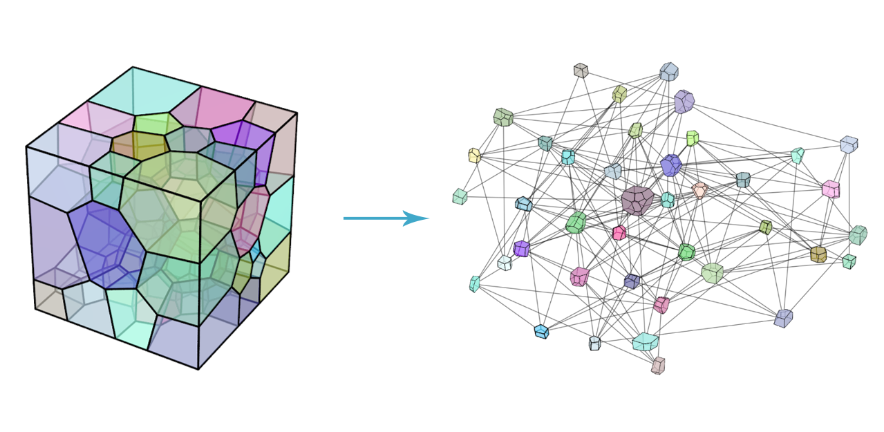
Figure 1: Polycrystal interpreted as a weighted connectivity graph. The graph is undirected and weighted at the nodes.

It can be difficult to directly incorporate either Euclidean or non-Euclidean data to a hand-crafted constitutive model. There have been attempts to infer information directly from scanned microstructual images using neural networks that utilize a convolutional layer architecture (CNN) (lubbers_inferring_2017). The endeavor to distill physically meaningful and interpertable features from scanned microstructural images stored in a Euclidean grid can be a complex and sometimes futile process. While recent advancements in convolutional neural networks have provided an effective mean to extract features that lead to extraordinary superhuman performance for image classification tasks (krizhevsky_imagenet_2012), similar success has not been recorded for mechanics predictions. This technical barrier could be attributed to the fact that feature vectors obtained from voxelized image data are highly sensitive to the grid resolution and noise. The robustness and accuracy also exhibit strong dependence on the number of dimensions of the feature vector space and the algorithms that extract the low-dimensional representations. In some cases, over-fitting and under-fitting can both cause the trained CNN extremely vulnerable to adversarial attacks and hence not suitable for high-risk, high-regret applications.

As demonstrated by (frankel_predicting_2019; jones2018machine), using images directly as additional input to our polycrystal energy functional approximator would be heavily contingent to the quality and size of the training pool. A large number of images, possibly in three dimensions, and in high enough resolution would be necessary to represent the latent features that will aid the approximator to distinguish successfully between different polycrystals. Using data in a Euclidean grid is an esoteric process that is dependent on empirical evidence that the current training sample holds adequate information to infer features useful in formulating a constitutive law. However, gathering that evidence can be a laborious process as it requires numerous trial and error runs and is weighed down by the heavy computational costs of performing filtering on Euclidean data (e.g. on high resolution 3D image voxels).

Graph representation of the data structures can provide a momentous head-start to overcome this very impediment. An example is the connectivity graph used in granular mechanics community where the formations and evolution of force chains are linked to macroscopic phenomena, such as shear band formation and failures (satake1992discrete; kuhn_stress-induced_2015; sun2013multiscale; tordesillas2014micromechanics; wang2019meta; wang2019updated). The distinct advantage of the graph representation of data, as showcased in the previous granular mechanics studies, is the high-level interpretability of the data structures. A knowledgeable user can employ domain expertise to craft graph structures that carry crucial relational information to solve the problem at hand. Designing graph structures - in terms of node connectivity, node and edge weights - can be highly expressive and exceptionally tailored to the task at hand. At the same time, by concisely selecting appropriate graph weights, one may incorporate only the essences of micro-structural data critical for mechanics predictions and hence more interpretable, flexible, economical and efficient than than incorporating feature spaces inferred from 3D voxel images. Furthermore, since one may easily rotational and transitional invariant data as weights, the graph approach is also advantageous for predicting constitutive responses that require frame indifference.

Currently, machine learning applications often employs two families of algorithms to take graphs as inputs, i.e., representation learning algorithms and graph neural networks. The former usually refer to unsupervised methods that convert graph data structures into formats or features that are easily comprehensible by machine learning algorithms (bengio2013representation). The later refer to neural network algorithms that accept graphs as inputs with layer formulations that can operate directly on graph structures (scarselli2008graph). Representation learning on graphs shares concepts with rather popular embedding techniques on text and speech recognition (mikolov_distributed_2013) to encode input in a vector format that can be utilized by common regression and classification algorithms. There has been multiple studies on encoding graph structures, spanning from the level of nodes (grover_node2vec:_2016) up to the level of entire graphs (perozzi_deepwalk:_2014; narayanan_graph2vec:_2017). Graph embedding algorithms, like DeepWalk (perozzi_deepwalk:_2014), utilize techniques such as random walks to ”read” sequences of neighbouring nodes resembling reading word sequences in a sentence and encode those graph data in an unsupervised fashion.

While these algorithms have been proven to be rather powerful and demonstrate competitive results in tasks like classification problems, they do come with disadvantages that can be limiting for use in engineering problems. Graph representation algorithms work very well on encoding the training dataset. However, they could be difficult to generalize and cannot accommodate dynamic data structures. This can be proven problematic for mechanics problems , where we expect a model to be as generalized as much as possible in terms of material structure variations (e.g. polycrystals, granular assemblies). Furthermore, representation learning algorithms can be difficult to combine with another neural network architecture for a supervised learning task in a sequential manner. In particular, when the representation learning is performed separately and independently from the supervised learning task that generates the the energy functional approximation, there is no guarantee that the clustering or classifications obtained from the representative learning is physically meaningful. Hence, the representation learning may not be capable of generating features that facilitates the energy functional prediction task in a completely unsupervised setting.

For the above reasons, we have opted for a hybrid neural network architecture that combines an unsupervised graph convolutional neural network with a multilayer perceptron to perform the regression task of predicting an energy functional. Both branches of our suggested hybrid architecture learn simultaneously from the same back-propagation process with a common loss function tailored to the approximated function. The graph encoder part - borrowing its name from the popular autoencoder architecture (vincent_extracting_2008) - learns and adjusts its weights to encode input graphs in a manner that serves the approximation task at hand. Thus, it does eliminate the obstacle of trying to coordinate the asynchronous steps of graph embedding and approximator training by parallel fitting both the graph encoder and the energy functional approximator with a common training goal (loss function).

As for notations and symbols in this current work, bold-faced letters denote tensors (including vectors which are rank-one tensors); the symbol ’$\cdot$’ denotes a single contraction of adjacent indices of two tensors (e.g. $\boldsymbol{a}\cdot\boldsymbol{b}=a_{i}b_{i}$ or $\boldsymbol{c}\cdot\boldsymbol{d}=c_{ij}d_{jk}$ ); the symbol ‘:’ denotes a double contraction of adjacent indices of tensor of rank two or higher ( e.g. $\boldsymbol{C}:\boldsymbol{\epsilon^{e}}$ = $C_{ijkl}\epsilon_{kl}^{e}$ ); the symbol ‘$\otimes$’ denotes a juxtaposition of two vectors (e.g. $\boldsymbol{a}\otimes\boldsymbol{b}=a_{i}b_{j}$) or two symmetric second order tensors (e.g. $(\boldsymbol{\alpha}\otimes\boldsymbol{\beta})_{ijkl}=\alpha_{ij}\beta_{kl}$). Moreover, $(\boldsymbol{\alpha}\oplus\boldsymbol{\beta})_{ijkl}=\alpha_{jl}\beta_{ik}$ and $(\boldsymbol{\alpha}\ominus\boldsymbol{\beta})_{ijkl}=\alpha_{il}\beta_{jk}$. We also define identity tensors $(\boldsymbol{I})_{ij}=\delta_{ij}$, $(\boldsymbol{I}^{4})_{ijkl}=\delta_{ik}\delta_{jl}$, and $(\boldsymbol{I}^{4}_{\text{sym}})_{ijkl}=\frac{1}{2}(\delta_{ik}\delta_{jl}+\delta_{il}\delta_{kj})$, where $\delta_{ij}$ is the Kronecker delta. As for sign conventions, unless specified otherwise, we consider the direction of the tensile stress and dilative pressure as positive.

2 Graphs as non-Euclidean descriptors for micro-structures

This section provides a detailed account on how to incorporate microstructural data represented by weighted graphs as descriptors for constitutive modeling. To aid readers not familiar with graph theory, we provide a brief review on some basic concepts of graph theory essential for understanding this research. The essential terminologies and definitions required to construct the graph descriptors can be found in Section 2.1. Following this review, we establish a method to translate the topological information of microstructures into various types of graphs (Section 2.2) and explain the properties of these graphs that are critical for the constitutive modeling tasks (Section 3).

2.1 Graph theory terminologies and definitions

In this section, a brief review of several terms of graph theory is provided to facilitate the illustration of the concepts in this current work. More elaborate descriptions can be found in (graham1989concrete; west2001introduction; bang2008digraphs):

Definition 1.

A graph is a two-tuple $\mathbb{G}=(\mathbb{V,E})$ where $\mathbb{V}=\{v_{1},...,v_{N}\}$ is a non-empty vertex set (also referred to as nodes) and $\mathbb{E}\subseteq\mathbb{V}\times\mathbb{V}$ is an edge set. To define a graph, there exists a relation that associates each edge with two vertices (not necessarily distinct). These two vertices are called the edge’s endpoints. The pair of endpoints can either be unordered or ordered.

Definition 2.

An undirected graph is a graph whose edge set $\mathbb{E}\subseteq\mathbb{V}\times\mathbb{V}$ connects unordered pairs of vertices together.

Definition 3.

A directed graph is a graph whose edge set $\mathbb{E}\subseteq\mathbb{V}\times\mathbb{V}$ connects ordered pairs of vertices together.

Definition 4.

A loop is an edge whose endpoint vertices are the same. When the all the nodes in the graph are in a loop with themselves, the graph is referred to as allowing self-loops.

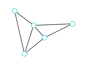
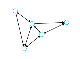
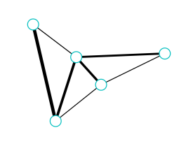
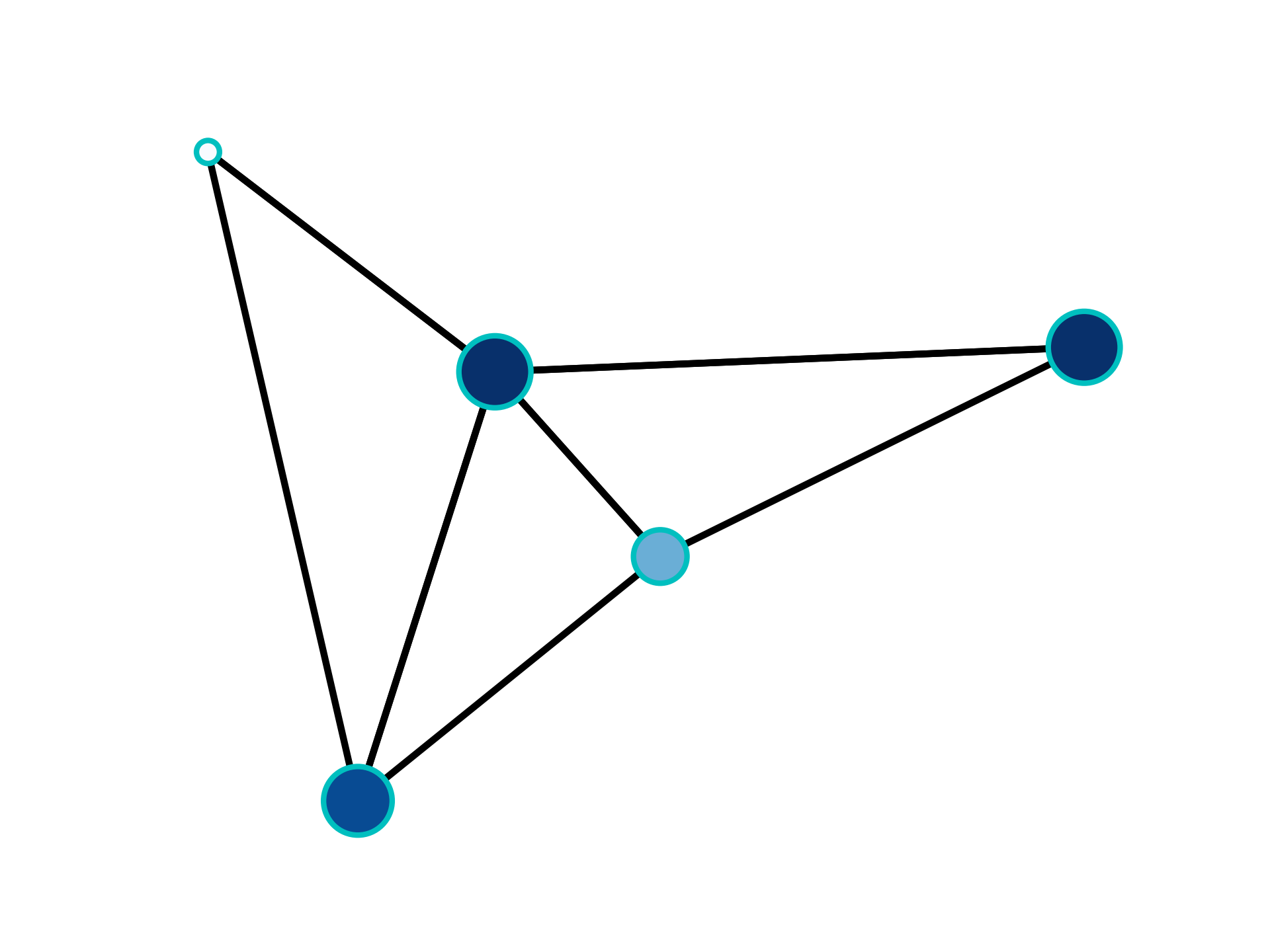
(a)	(b)	(c)	(d)

Figure 2: Different types of graphs. (a) Undirected (simple) binary graph (b) Directed binary graph (c) Edge-weighted undirected graph (d) Node-weighted undirected graph.

Definition 5.

Multiple edges are edges having the same pair of endpoint vertices.

Definition 6.

A simple graph is a graph that does not have loops or multiple edges.

Definition 7.

Two vertices that are connected by an edge are referred to as adjacent or as neighbors.

Definition 8.

The term weighted graph traditionally refers to graph that consists of edges that associate with edge-weight function $w_{ij}:\mathbb{\mathbb{E}}\rightarrow\mathbb{R}^{n}\enskip\text{with}\enskip(i,j)\in\mathbb{E}$ that maps all edges in $\mathbb{E}$ onto a set of real numbers. $n$ is the total number of edge weights and each set of edge weights can be represented by a matrix $\boldsymbol{W}$ with components $w_{ij}$.

In this current work, unless otherwise stated, we will be referring to weighted graphs as graphs weighted at the vertices - each node carries information as a set of weights that quantify features of microstructures. All vertices are associated with a vertex-weight function $f_{v}:\mathbb{\mathbb{V}}\rightarrow\mathbb{R}^{D}\enskip\text{with}\enskip v\in\mathbb{V}$ that maps all vertices in $\mathbb{V}$ onto a set of real numbers, where $D$ is the number of weights - features. The node weights can be represented by a $N\times D$ matrix $\boldsymbol{X}$ with components $x_{ik}$, where the index $i\in[1,...,N]$ represents the node and the index $k\in[1,...,D]$ represents the type of node weight - feature.

Definition 9.

A graph whose edges are unweighted ($w_{\epsilon}=1\enskip\forall\epsilon\in\mathbb{E}$) can be called a binary graph.

To facilitate the description of graph structures, several terms for representing graphs are introduced:

Definition 10.

The adjacency matrix $\boldsymbol{A}$ of a graph $\mathbb{G}$ is the $N\times N$ matrix in which entry $\alpha_{ij}$ is the number of edges in $\mathbb{G}$ with endpoints $\{v_{i},v_{j}\}$.

Definition 11.

If the vertex $v$ is an endpoint of edge $\epsilon$, then $v$ and $\epsilon$ are incident. The degree $d$ of a vertex $v$ is the number of incident edges. The degree matrix $\boldsymbol{D}$ of a graph $\mathbb{G}$ is the $N\times N$ diagonal matrix with diagonal entries $d_{ii}$ equal to the degree of vertex $v_{i}$.

Definition 12.

The unnormalized Laplacian operator $\boldsymbol{\Delta}$ is defined such that:

$$(\boldsymbol{\Delta}f)_{i} =\sum_{j:(i,j)\in\mathbb{E}}w_{ij}(f_{i}-f_{j})$$ (2)

$$=f_{i}\sum_{j:(i,j)\in\mathbb{E}}w_{ij}-\sum_{j:(i,j)\in\mathbb{E}}w_{ij}f_{j}.$$ (3)

By writing the equation above in matrix form, the unnormalized Laplacian matrix $\boldsymbol{\Delta}$ of a graph $\mathbb{G}$ is the $N\times N$ positive semi-definite matrix defined as $\boldsymbol{\Delta}=\boldsymbol{D}-\boldsymbol{W}$.

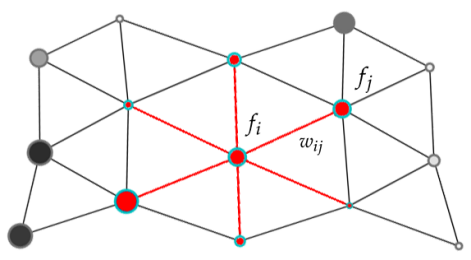
Figure 3: The graph Laplacian operator $\boldsymbol{\Delta}$ describes the difference between a value $f$ at a node and its local average.

In this current work, binary graphs will be used, thus, the equivalent expression is used for the unnomrmalized Laplacian matrix $\boldsymbol{L}$, defined as $\boldsymbol{L}=\boldsymbol{D}-\boldsymbol{A}$ with the entries $l_{ij}$ calculated as:

$$\l_{ij}=\left\{\begin{array}[]{ll}d_{i},&i=j\\ -1,&i\neq j\enskip\text{and}\enskip v_{i}\enskip\text{is adjacent to}\enskip v_{j}\\ 0,&\text{otherwise}.\\ \end{array}\right.$$ (4)

Definition 13.

For binary graphs, the symmetric nomrmalized Laplacian matrix $\boldsymbol{L^{\text{sym}}}$ of a graph $\mathbb{G}$ is the $N\times N$ matrix defined as:

$$\boldsymbol{L^{\text{sym}}}=\boldsymbol{D}^{-\frac{1}{2}}\boldsymbol{L}\boldsymbol{D}^{-\frac{1}{2}}=\boldsymbol{I}-\boldsymbol{D}^{-\frac{1}{2}}\boldsymbol{A}\boldsymbol{D}^{-\frac{1}{2}}.$$ (5)

The entries $l^{\text{sym}}_{ij}$ of the matrix $\boldsymbol{L^{\text{sym}}}$ can also be calculated as:

$$\l^{\text{sym}}_{ij}=\left\{\begin{array}[]{ll}1,&i=j\enskip\text{and}\enskip d_{i}\neq 0\\ -(d_{i}d_{j})^{-\frac{1}{2}},&i\neq j\enskip\text{and}\enskip v_{i}\enskip\text{is adjacent to}\enskip v_{j}\\ 0,&\text{otherwise}.\\ \end{array}\right.$$ (6)

2.2 Polycrystals represented as node-weighted undirected graphs

Representing microstructural data as weight graphs requires pooling, a down-sampling procedure to converts field data of a specified domain into low-dimensional features that preserve the important information. One of the most intuitive pooling is to infer the grain connectivity graph from an micro-CT image (jaquet2013estimation; wang2016identifying) or realization of micro-structures generated from software packages such as Neper or Cubit (quey_large-scale_2011; salinger2016albany). In this work, we treat each individual crystal grain as as node or vertex in a graph, and create an edge for each in-contact grain pair. The sets of the nodes and edges, $\mathbb{B}$ and $\mathbb{E}$ collectively forms as a graph (cf. Def. 1). Without adding any weight, this graph can be represented by a binary graph (cf. Def. 9) of which the binary weight for each edge indicates whether the two grains are in contact, as shown in Figure 2. While the unweighted graph can be used incorporated into the machine learning process, additional information of the microstructures can be represented by weights assigned on the nodes and edges of a graph that represents an assembles. In this current work, the database included information on the volume, the orientation (in Euler angles), the total surface area, the number of faces, the numbers of neighbors, as well as other shape descriptors (convexity, equivalent diameter, etc) for every crystal in the polycrystals - all of which could be assigned as node weights in the connectivity graph. Information was also available on the nature of contact between grains - such as the surface and the angle of contact - which could be used as weights for the edges of the graph. While this current work is solely focused on node weighted graphs, future work could employ algorithms that utilize edge weights as well to generate more robust microstructure predictors.

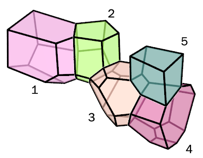
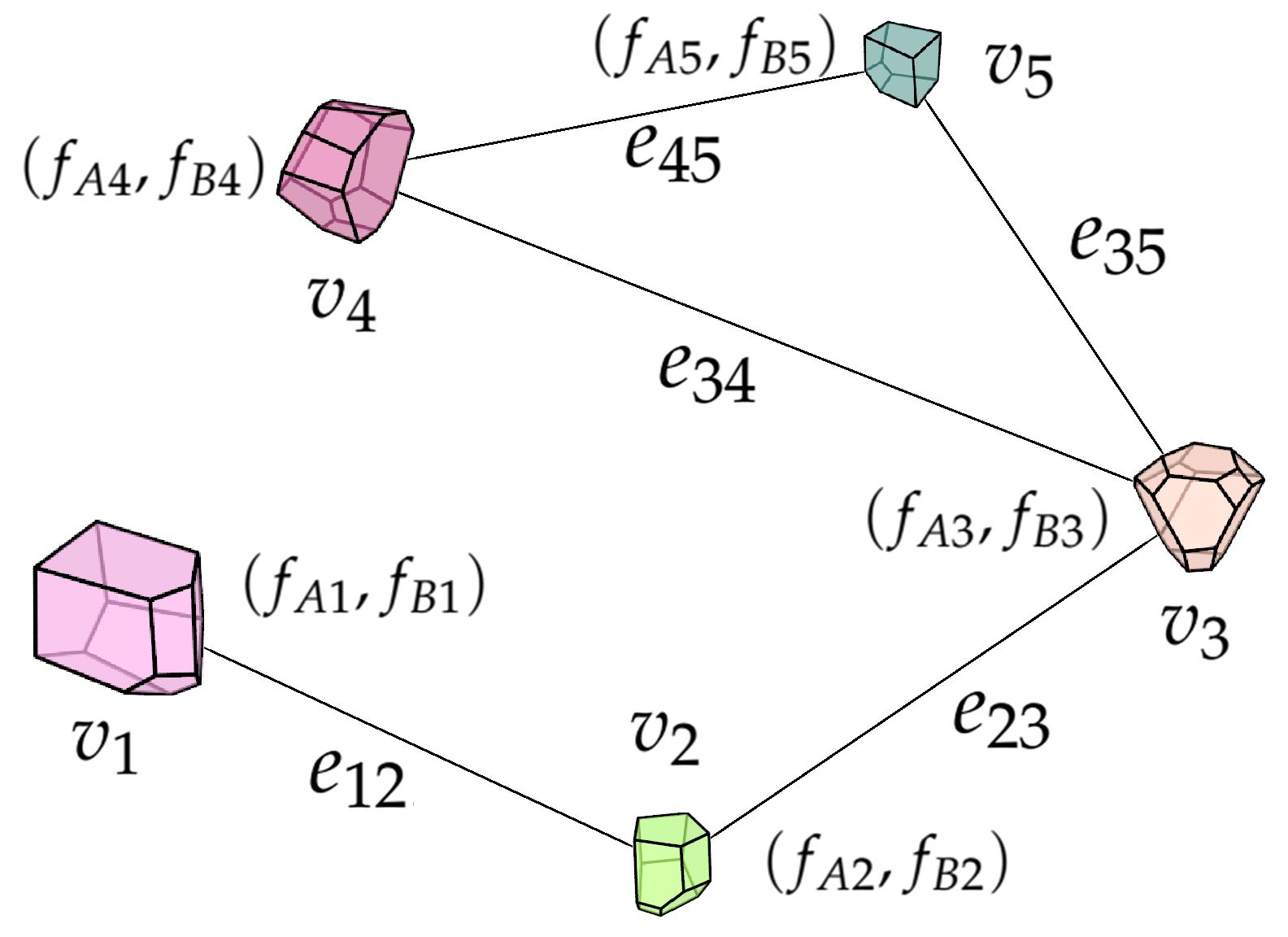
(a)	(b)

Figure 4: A sub-sample of a polycrystal (a) represented as an undirected weighted graph (b). If two crystals in the formation share an edge, their nodes are also connected in the graph. Each node is weighted by two features $f_{A}$ and $f_{B}$.

To demonstrate how graphs used to represent a polycrystalline assembles are generated, we introduced a simple example where an assembly consist of 5 crystals shown in Fig. 4(a) is converted into a node-weighted graph. Each node of the graph represents a crystal. An edge is defined between two nodes if they are connected - share a surface. The graph is undirected meaning that there is no direction specified for the edges. The vertex set $\mathbb{V}$ and edge set $\mathbb{E}$ for this specific graph are $\mathbb{V}=\{v_{1},v_{2},v_{3},v_{4},v_{5}\}$ and $\mathbb{E}=\{e_{12},e_{23},e_{34},e_{35},e_{45}\}$ respectively.

An undirected graph can be represented by an adjacency matrix $\boldsymbol{A}$ (cf. Def. 10) that holds information for the connectivity of the nodes. The entries of the adjacency matrix $\boldsymbol{A}$ in this case are binary - each entry of the matrix is 0 if an edge does not exist between two nodes and 1 if it does. Thus, for the example in Fig. 4, crystals 1 and 2 are connected so the entries $(1,2)$ and $(2,1)$ of the matrix $\boldsymbol{A}$ would be 1, while crystals 1 and 3 are not so the entries $(1,3)$ and $(3,1)$ will be 0 and so on. If the graph allows self-loops, then the entries in the diagonal of the matrix are equal to 1 and the adjacency matrix with self-loops is defined as $\boldsymbol{\hat{A}}=\boldsymbol{A}+\boldsymbol{I}$. The complete symmetric matrices $\boldsymbol{A}$ and $\boldsymbol{\hat{A}}$ for this example will be:

$$\boldsymbol{A}=\left[\begin{array}[]{ccccc}0&1&0&0&0\\ 1&0&1&0&0\\ 0&1&0&1&1\\ 0&0&1&0&1\\ 0&0&1&1&0\end{array}\right]$$

$$\boldsymbol{\hat{A}}=\boldsymbol{A}+\boldsymbol{I}=\left[\begin{array}[]{ccccc}1&1&0&0&0\\ 1&1&1&0&0\\ 0&1&1&1&1\\ 0&0&1&1&1\\ 0&0&1&1&1\end{array}\right]$$

A diagonal degree matrix $\boldsymbol{D}$ can also useful to describe a graph representation. The degree matrix $\boldsymbol{D}$ only has diagonal terms that equal the number of neighbors of the node represented in that row. The diagonal terms can simply be calculated by summing all the entries in each row of the adjacency matrix. It is noted that, when self-loops are allowed, a node is a neighbor of itself, thus it must be added to the number of total neighbors for each node. The degree matrix $\boldsymbol{D}$ for the example graph in Fig. 4 would be:

$$\boldsymbol{D}=\left[\begin{array}[]{ccccc}1&0&0&0&0\\ 0&2&0&0&0\\ 0&0&3&0&0\\ 0&0&0&2&0\\ 0&0&0&0&2\end{array}\right]$$

The polycrystal connectivity graph can be represented by its graph Laplacian matrix $\boldsymbol{L}$ - defined as $\boldsymbol{L}=\boldsymbol{D}-\boldsymbol{A}$, as well as the normalized symmetric graph Laplacian matrix $\boldsymbol{L^{\text{sym}}}=\boldsymbol{D}^{-\frac{1}{2}}\boldsymbol{L}\boldsymbol{D}^{-\frac{1}{2}}$. The two matrices for the example of Fig. 4 are calculated below:

$$\boldsymbol{L}=\left[\begin{array}[]{ccccc}1&-1&0&0&0\\ -1&2&-1&0&0\\ 0&-1&3&-1&-1\\ 0&0&-1&2&-1\\ 0&0&-1&-1&2\end{array}\right]$$

$$\boldsymbol{L^{\text{sym}}}=\left[\begin{array}[]{ccccc}1&-\frac{\sqrt{2}}{2}&0&0&0\\ -\frac{\sqrt{2}}{2}&1&-\frac{\sqrt{6}}{6}&0&0\\ 0&-\frac{\sqrt{6}}{6}&1&-\frac{\sqrt{6}}{6}&-\frac{\sqrt{6}}{6}\\ 0&0&-\frac{\sqrt{6}}{6}&1&-\frac{1}{2}\\ 0&0&-\frac{\sqrt{6}}{6}&-\frac{1}{2}&1\end{array}\right]$$

Assume that, for the example in Fig. 4,there is information available for two features $A$ and $B$ for each crystal in the graph that will be used as node weights - this could be the volume of each crystal, the orientations and so on. The node weights for each feature can be described as a vector, $\boldsymbol{f}_{A}=(f_{A1},f_{A2},f_{A3},f_{A4},f_{A5})$ and $\boldsymbol{f}_{B}=(f_{B1},f_{B2},f_{B3},f_{B4},f_{B5})$, such that each component of the vector corresponds to a feature of a node. The node features can all be represented in a feature matrix $\boldsymbol{X}$ where each row corresponds to a node and each column corresponds to a feature. For the example in question, the feature matrix would be:

$$\boldsymbol{X}=\left[\begin{array}[]{cc}f_{A1}&f_{B1}\\ f_{A2}&f_{B2}\\ f_{A3}&f_{B3}\\ f_{A4}&f_{B4}\\ f_{A5}&f_{B5}\end{array}\right]$$

While the connectivity graph appears as the most straightforward approach to pooling polycrystal microstuctural information in a non-Euclidean domain, this is not necessarily valid for other applications. While, for a polycrystal material, the connectivity graph could possibly remain constant with time, this would not be the case for a granular material (grain contacts). Another graph descriptor should be constructed that would evolve with time. For the flow modelling of a porous material, other graph descriptors could be more important (pore space, flow network).

3 Deep learning on graphs

Machine learning often involves algorithms designed to statistically estimate highly complex functions by learning from data. Some common applications in machine learning are those of regression and classification. A regression algorithm attempts to make predictions of a numerical value provided some input data. A classification algorithm attempts to assign a label to an input and place it to one or multiple classes / categories that it belongs to. Classification tasks can be supervised, if information for the true labels of the inputs are available during the learning process. Classification tasks can also be unsupervised, if the algorithm is not exposed to the true labels of the input during the learning process but attempts to infer labels for the input by learning properties of the input dataset structure. The hybrid geometric learning neural network introduced in this work performs simultaneously an unsupervised classification of polycrystal graph structures and the regression of an anisotropic elastic energy potential functional.

In the following sections, we firstly introduce several basic machine learning and deep neural network terminologies that will be encountered in this work (Section 3.1). We provide an overview the fundamental deep learning architecture of the multilayer-perceptron (MLP) - that will also carry the regression part of the hybrid architecture. In Section 3.2, we introduce the novel application of the graph convolution technique that will carry out the unsupervised classification of the polycrystals. Finally, in Section 3.3, we introduce our hybrid architecture that combines these two architectures to perform their tasks simultaneously.

3.1 Deep learning for regression

To describe a machine learning algorithm, a dataset, a model, a loss function, and an optimization procedure must be specified. The dataset refers to the total samples that are available for the training and testing of a machine learning algorithm. A dataset is commonly split in training, validation and testing sets. The training set will be used for the algorithm to be trained on and learned from. The validation set is used, while the learning process takes place, to evaluate the the learning procedure and optimize the learning algorithm. The testing set consists of unseen data - data exclusive from the training set - to test the algorithm’s blind prediction capabilities, after the learning process is complete. A (parametric) model refers to the structure that holds the parameters that describe the learned function - the number of these parameters are finite and fixed before any data is observed. A loss function (usually also referred to as cost, error or objective function) refers to a metric that must be either minimized or maximized during learning for the learning to be successful - the values of this function drive the learning process. The optimization procedure refers the numerical method utilized to find the optimal parameters of the model that minimize or maximize the loss function. A more complete discussion on machine learning and neural networks can be found in, for instance, (Goodfellow-et-al-2016).

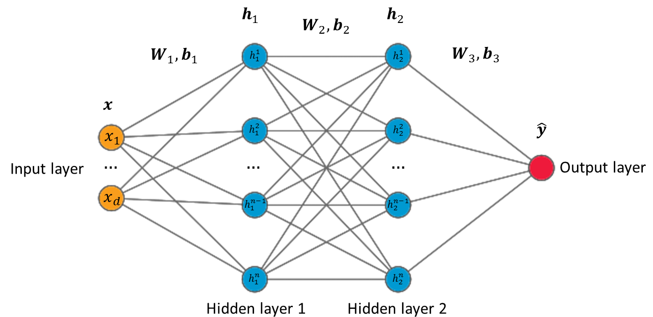
Figure 5: A two-layer perceptron. The input vector $\boldsymbol{x}$ has $d$ features, each of the two hidden layers $h_{l}$ has $m$ neurons.

A subset of machine learning algorithms that can learn from high-dimensional data are the artificial neural network (ANN) and deep learning algorithms. Inspired by the structure and function of biological neural networks, ANNs can learn to perform highly complex tasks on large datasets, such as those of image, audio, and video data. One of the simplest ANN architectures would be the multilayer perceptron (MLP) or often called feed forward neural network. The formulation for the two-layer perceptron in Fig. 5, similar to the one that is also used in this work, is presented below as a series of matrix multiplications:

$$\textbf{z}_{1} =\textbf{x}\textbf{W}_{1}+\textbf{b}_{1}$$ (7)

$$\textbf{h}_{1} =\sigma(\textbf{z}_{1})$$ (8)

$$\textbf{z}_{2} =\textbf{h}_{1}\textbf{W}_{2}+\textbf{b}_{2}$$ (9)

$$\textbf{h}_{2} =\sigma(\textbf{z}_{2})$$ (10)

$$\textbf{z}_{\text{out}} =\textbf{h}_{2}\textbf{W}_{3}+\textbf{b}_{3}$$ (11)

$$\hat{\textbf{y}} =\sigma_{\text{out}}(\textbf{z}_{\text{out}}).$$ (12)

In the above formulation, the input vector $\boldsymbol{x}_{l}$ contains the features of a sample, the weight matrix $\boldsymbol{W}_{l}$ contains the weights - parameters of the network, and $\boldsymbol{b}_{l}$ is the bias vector for every layer. The function $\sigma$ is the chosen activation function for the hidden layers. In the current work, the MLP hidden layers have the ELU function as an activation function, defined as:

$$\text{ELU}(\alpha)=\left\{\begin{array}[]{ll}e^{\alpha}-1,&\alpha<0\\ \alpha,&\alpha\geq 0.\\ \end{array}\right.$$ (13)

The vector $\boldsymbol{h}_{l}$ contains the activation function values for every neuron in the hidden layer. The vector $\hat{\boldsymbol{y}}$ is the output vector of the network with linear activation $\sigma_{\text{out}}(\bullet)=(\bullet)$.

If $\boldsymbol{y}$ are the true function values corresponding to the inputs $\boldsymbol{x}$, then the MLP architecture could be simplified as an approximator function $\hat{\boldsymbol{y}}=\hat{\boldsymbol{y}}(\boldsymbol{x}|\boldsymbol{W},\boldsymbol{b})$ with inputs $\boldsymbol{x}$ parametrized by $\boldsymbol{W}$ and $\boldsymbol{b}$, such that:

$$\boldsymbol{W}^{\prime},\boldsymbol{b}^{\prime}=\operatorname*{argmin}_{\boldsymbol{W},\boldsymbol{b}}\ell(\hat{\boldsymbol{y}}(\boldsymbol{x}|\boldsymbol{W},\boldsymbol{b}),\boldsymbol{y}),$$ (14)

where $\boldsymbol{W}^{\prime}$ and $\boldsymbol{b}^{\prime}$ are the optimal weights and biases of the neural network that arrive from the optimization - training process such that a defined loss function $\ell$ is minimized. The loss functions used in this work are discussed in Section 4.

The fully-connected (Dense) layer that is used as the hidden layer that is used for a standard MLP architecture has the following general formulation:

$$\boldsymbol{h}^{(l+1)}_{\text{dense}}=\sigma(\boldsymbol{h}^{(l)}\boldsymbol{W}^{(l)}+\boldsymbol{b}^{(l)}).$$ (15)

The architecture described above will constitute the energy functional regression branch of the hybrid architecture described in Section 3.3. It is noted, as it will be discussed later in Section LABEL:sec:graph_based_model, that this architecture would be sufficient to predict the energy functional for a single polycrystal with the strain being the sole input and the energy functional the output. To predict the complex behavior of multiple polycrystals, the hybrid architecture is introduced in the following sections.

3.2 Graph convolution network for unsupervised classification of polycrystals

Geometric learning refers to the extension of previously established neural network techniques to graph structures and manifold-structured data. Graph Neural Networks (GNN) refers to a specific type of neural networks architectures that operate directly on graph structures. An extensive summary of different graph neural network architectures currently developed can be found in (wu_comprehensive_2019). Graph convolution networks (GCN) (defferrard_convolutional_2016; kipf_semi-supervised_2017) are variations of graph neural networks that bear similarities with the highly popular convolutional neural network (CNN) algorithms, commonly used in image processing (lecun_gradient-based_1998; krizhevsky_imagenet_2012). The mutual term convolutional refers to use of filter parameters that are shared over all locations in the graph similar to image processing. Graph convolution networks are designed to learn a function of features or signals in graphs $\mathbb{G}=(\mathbb{V,E})$ and they have demonstrated competitive scores at tasks of classification (kipf_semi-supervised_2017; simonovsky2017dynamic).

In this current work, we utilize a GCN layer implementation similar to that introduced in (kipf_semi-supervised_2017). The implementation is based on the open-source neural network library Keras (chollet2015keras) and the open-source library on graph neural networks Spektral (noauthor_spektral_nodate). The GCN layers will be the ones that learn from the polycrystal connectivity graph information. A GCN layer accepts two inputs, a symmetric normalized graph Laplacian matrix $\boldsymbol{L^{\text{sym}}}$ and a node feature matrix $\boldsymbol{X}$ as described in Section 2.1. The matrix $\boldsymbol{L^{\text{sym}}}$ holds the information about the graph structure. The matrix $\boldsymbol{X}$ holds information about the features of every node in the graph - every crystal in the polycrystal. In matrix form, the GCN layer has the following structure:

$$\boldsymbol{h}^{(l+1)}_{\text{GCN}}=\sigma(\boldsymbol{L^{\text{sym}}}\boldsymbol{h}^{(l)}\boldsymbol{W}^{(l)}+\boldsymbol{b}^{(l)}).$$ (16)

In the above formulation, $\boldsymbol{h}^{l}$ is the output of a layer $l$. For $l=0$, the first GCN layer of the network accepts the graph features as input such that $\boldsymbol{h}^{0}=\boldsymbol{X}$. For $l>1$, $\boldsymbol{h}$ represents a higher dimension representation of the graph features that are produced from the convolution function, similar to a CNN layer. The function $\sigma$ is a non-linear activation function. In this work, the GCN layers use the Rectified Linear Unit activation function, defined as $ReLU(\bullet)=\max(0,\bullet)$. The weight matrix $\boldsymbol{W}^{l}$ and bias vector $\boldsymbol{b}^{l}$ are the parameters of the layer that will be optimized during training.

The matrix $\boldsymbol{L^{\text{sym}}}$ has dimensions $N\times N$, where $N$ is the number of nodes in the graph - crystalline grain in the polycrystal. The node feature matrix $\boldsymbol{X}$ has dimensions of $N\times D$ where $N$ is the number of nodes in the graph and $D$ is the number of used input features (node weights). In this work, four crystal features where used as node weights (the volume and the three Euler angles for each crystal), thus, $D=4$. Unweighted graphs can be used too - in that case the feature matrix is just the identity matrix $\boldsymbol{X}=\boldsymbol{I}$. The matrix $\boldsymbol{L^{\text{sym}}}$ acts as an operator on the node feature matrix $\boldsymbol{X}$ so that, for every node, the sum of every neighbouring node features and the node itself is accounted for. In order to include the features of the node itself, the matrix $\boldsymbol{L^{\text{sym}}}$ comes by using Equation 5 with the binary adjacency matrix $\boldsymbol{\hat{A}}$ allowing self-loops and the equivalent degree matrix $\boldsymbol{D}$. Using the normalized laplacian matrix $\boldsymbol{L^{\text{sym}}}$, instead of the adjacency matrix $\boldsymbol{\hat{A}}$, for feature filtering remedies possible numerical instabilites and vanishing / exploding gradient issues when using the GCN layer in deep neural networks.

This type of spatial filtering can be of great use in constitutive modelling. In the case of the polycrystals, for example, the neural network model does not solely learn on the features of every crystal separately. It also learns by aggregating the features of the neighboring crystals in the graph and potentially uncover a behavior that stems from the feature correlation between different nodes. This property deems this filtering function a considerable candidate for learning on spatially heterogeneous material structures.

3.3 Hybrid neural network architecture for simultaneous unsupervised classification and regression

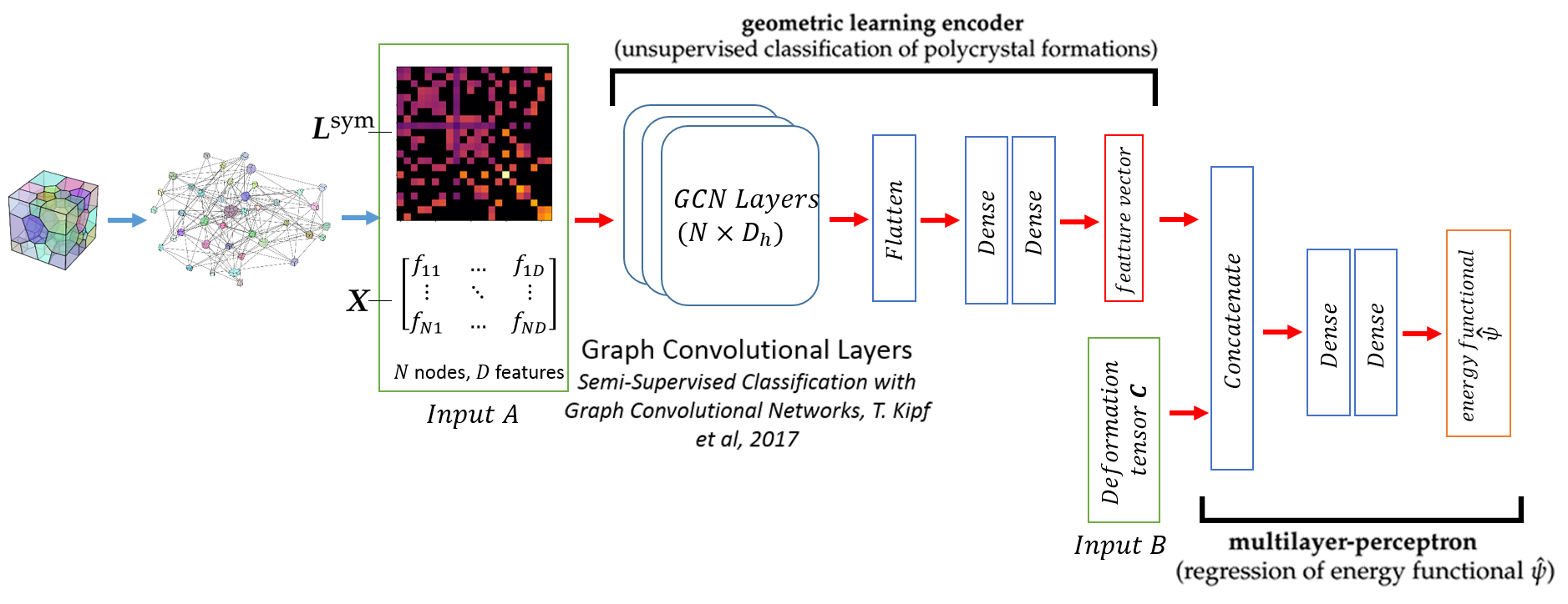
Figure 6: Hybrid neural network architecture. The network is comprised of two branches - a graph convolutional encoder and a multi-layer perceptron. The first branch accepts the graph structure (normalized Laplacian $\boldsymbol{L^{\text{sym}}}$) and graph weights (feature matrix $\boldsymbol{X}$) (Input A) as inputs and outputs an encoded feature vector. The second branch accepts the concatenated encoded feature vector and the right Cauchy–Green deformation tensor $\boldsymbol{C}$ in Voigt notation (Input B) as inputs and outputs the energy functional $\hat{\psi}$ prediction.

The hybrid network architecture employed in this current work is designed to perform two tasks simultaneously, guided by a common objective function. The first task is the unsupervised classification of the connectivity graphs of the polycrystals. This is carried through by the first branch of the hybrid architecture that resembles that of a convolutional encoder, commonly used in image classification (lecun_gradient-based_1998; krizhevsky_imagenet_2012) and autoencoders (vincent_extracting_2008). However, the convolutional layers are now following the aforementioned GCN layer formulation. A convolutional encoder passes a complex structure (i.e images, graphs) through a series of filters to can generate a higher level representation and encode - compress the information in a structure of lower dimensions (i.e. a vector). It is common practice, for example, in image classification (krizhevsky_imagenet_2012), to pass an image through a series of stacked convolutional layers, that increase the feature space dimensionality, and then encode the information in a vector through a multilayer perceptron - a series of stacked fully connected layers. The weights of the every layer in the network are optimized using a loss function (usually categorical cross-entropy) so that the output vector matches the classification labels of the input image.

A similar concept is employed for the geometric learning encoder branch of the hybrid architecture. This branch accepts as inputs the normalized graph Laplacian and the node feature matrices. The two convolutional layers read the graph features and increase the dimensionality of the node features. These features are then and flattened and then fed to two fully connected layers that encode the graph information in a feature vector. The encoded feature vector dense layer can have a linear activation function, similar to regression problems, or a softmax activation function with a range of 0 to 1, similar to multi-label classification problems. Both activation functions have been tested and appear to have comparable results.

The second task performed by the hybrid network is a regression task - the prediction of the energy functional. The architecture of this branch of the network follows that of a simple feed-forward network with two hidden fully connected layers, similar to the one described in Section 3.1. The input of this branch is the encoded feature vector, arriving from the geometric learning encoder branch, concatenated with the second order right Cauchy–Green deformation tensor $\boldsymbol{C}$ in Voigt vector notation. The output of this branch is the predicted energy functional $\hat{\psi}$. It is noted that in this current work, an elastic energy functional is predicted and the not history dependent behavior can be adequately mapped with feed-forward architectures. Applications of geometric learning on plastic behavior will be the object of future work and will require recurrent network architectures that can capture the material’s behavior history, similar to (wang_multiscale_2018).

The layer weights of these two branches are updated in tandem with a common back-propagation algorithm and an objective function that rewards the better energy functional and stress field predictions, using a Sobolev training procedure, described in Section 4.

While this hybrid network architecture provides a promising aspect for incorporating structural data in the form of graphs, there are still several shortcomings that should be addressed in future work. The GCN algorithm itself is not inductive - it cannot introduce new nodes and generalize in terms of the graph structure very efficiently. It is, thus, suggested that the graph structures used in training are statistically similar to each other, so that with adequate regularization the model can generalize on unseen but similar structures. This is the reason why in this current work we focus on making predictions on families of polycrystals with statistically similar crystal number distributions. Simultaneously, we implement rigorous methods of regularization on the graph encoder branch of the hybrid architecture, in the form of Dropout layers (srivastava_dropout:_2014) and $L_{2}$ regularization. We have discovered that regularization techniques provide a competent method for combating overfitting issues, addressed later in this work. This work is a first attempt to utilizing geometric learning in material mechanics and model refinement will be considered when approaching more complex problems in the future (e.g. history dependent plasticity problems).

4 Sobolev training for hyperelastic energy functional predictions

In principle, forecast engines for elastic constitutive responses are trained by (1) an energy-conjugate pair of stress and strain measures (ghaboussi_knowledge-based_1991; wang_multiscale_2018; lefik_artificial_2009), (2) a power-conjugate pair of stress and strain rates (liu_deep_2019) and (3) a pair of strain measure and Helmholtz stored energy (lu_data-driven_2019; huang_predictive_2019). While options (1) and (2) can both be simple and easy to train once the proper configuration of the neural networks are determined, one critical drawback is that the resultant model may predict non-convex energy response and exhibit ad-hoc path-dependence (borja1997coupling).

An alternative is to introduce supervised learning that takes strain measure as input and output the stored energy functional. This formulation leads to the so-called hyperelastic or Green-elastic material, which postulate the existence of a Helmholtz free-energy function (holzapfel_new_2000). The concept of learning a free energy function as a mean to describe multi-scale materials has been previously explored (le2015computational; teichert2019machine_a). However, without direct control of the gradient of the energy functional, the predicted stress and elastic tangential operator may not be sufficiently smooth unless the activation functions and the architecture of the neural network are carefully designed. To rectify the drawbacks of these existing options, we leverage the recent work on Sobolev training (czarnecki_sobolev_2017) in which we incorporate both the stored elastic energy functional and the derivatives (i.e. conjugate stress tensor) into the loss function such that the objective of the training is not solely minimizing the errors of the energy predictions but the discrepancy of the stress response as well.

Traditional deep learning regression algorithms aim to train a neural network to approximate a function by minimizing the discrepancy between the predicted values and the benchmark data. However, the metric or norm used to measure discrepancy is often the $L_{2}$ norm, which does not regularize the derivative or gradients or the learned function. When combined with the types of activation functions that include high-frequency basis, the learned function may exhibit spurious oscillation and hence not suitable for training hyperelastic energy function that requires smoothness for the first and second derivatives.

Sobolev training we adopted from czarnecki_sobolev_2017 is designed to maximize the utilization of data by leveraging the available additional higher order data in the form of higher order constraints in the training objective function. In the Sobolev training, objective functions are constructed for minimizing the $H^{K}$ Sobolev norms of the corresponding Sobolev space. Recall that a Sobolev space refers to the space of functions equipped with norm comprised of $L^{p}$ norms of the functions and their derivatives up to a certain order $K$.

Since it has been shown that neural networks with the ReLU activation function (as well as functions similar to that) can be universal approximators for $C^{1}$ functions in a Sobolev space (sonoda2017neural), our goal here is to directly predict the elastic energy functional by using the Sobolev norm as loss function to train the hybrid neural network models.

This current work focuses on the prediction of an elastic stored energy functional listed in Eq. 1, thus, for simplicity, the superscript $e$ (denoting elastic behavior) will be omitted for all energy, strain, stress, and stiffness scalar and tensor values herein. In the case of the simple MLP feed- forward network, the network can be seen as an approximator function $\hat{\psi}=\hat{\psi}(\boldsymbol{C}|\boldsymbol{W},\boldsymbol{b})$ of the true energy functional $\psi$ with input the right Cauchy–Green deformation tensor $\boldsymbol{C}$, parametrized by weights $\boldsymbol{W}$ and biases $\boldsymbol{b}$. In the case of the hybrid neural network architecture, the network can be seen as an approximator function $\hat{\psi}=\hat{\psi}(\mathbb{G},\boldsymbol{C}|\boldsymbol{W},\boldsymbol{b})$ of the true energy functional $\psi$ with input the polycrystal connectivity graph information (as described in Fig. 6) and the tensor $\boldsymbol{C}$, parametrized by weights $\boldsymbol{W}$ and biases $\boldsymbol{b}$. The first training objective in Equation 17 for the training samples $i\in[1,...,N]$ is modelled after an $L_{2}$ norm, constraining only $\psi$:

$$\boldsymbol{W}^{\prime},\boldsymbol{b}^{\prime}=\operatorname*{argmin}_{\boldsymbol{W},\boldsymbol{b}}\left(\frac{1}{N}\sum_{i=1}^{N}\left\lVert\psi_{i}-\hat{\psi}_{i}\right\rVert^{2}_{2}\right).$$ (17)

The second training objective in Equation 18 for the training samples $i\in[1,...,N]$ is modelled after an $H_{1}$ norm, constraining both $\psi$ and its first derivative with respect to $\boldsymbol{C}$ - i.e. one half of the 2nd Piola Kirchhoff stress tensor $\boldsymbol{S}$:

$$\boldsymbol{W}^{\prime},\boldsymbol{b}^{\prime}=\operatorname*{argmin}_{\boldsymbol{W},\boldsymbol{b}}\left(\frac{1}{N}\sum_{i=1}^{N}\left\lVert\psi_{i}-\hat{\psi}_{i}\right\rVert^{2}_{2}+\left\lVert\frac{\partial\psi_{i}}{\partial\boldsymbol{C}}-\frac{\partial\hat{\psi}_{i}}{\partial\boldsymbol{C}}\right\rVert^{2}_{2}\right),$$ (18)

where in the above:

$$\boldsymbol{S}=2\frac{\partial\psi}{\partial\boldsymbol{C}}.$$ (19)

It is noted that higher order objective functions can be constructed as well, such as an $H_{2}$ norm constraining the predicted $\hat{\psi}$, stress, and stiffness values. This would be expected to procure even more accurate $\hat{\psi}$ results, smoother stress predictions and more accurate stiffness predictions. However, since a neural network is a combination of linear functions - the second order derivative of the ReLU and its adjacent activation functions is zero, it becomes innately difficult to control the second order derivative during training, thus in this work we mainly focus on the first order Sobolev method. In case it is desired to control the behavior of the stiffness tensor, a first order Sobolev training scheme can be designed with strain as input and stress as output. The gradient of this approximated relationship would be the stiffness tensor. This experiment would also be meaningful and useful in finite element simulations.

Figure 7: Schematic of the training procedure of a hyperelastic material surrogate model with the right Cauchy–Green deformation tensor $\boldsymbol{C}$ as input and the energy functional $\hat{\psi}$ as output. A Sobolev trained surrogate model will output smooth $\hat{\psi}$ predictions and the gradient of the model with respect to $\boldsymbol{C}$ will be a valid stress tensor $\hat{\boldsymbol{S}}$.

It is noted that, in this current work, the Sobolev training is implemented using the available stress information as the higher order constraint, assuring that the predicted stress tensors are accurate component-wise. In simpler terms, the $H_{1}$ norm constrains every single component of the second order stress tensor. It is expected that this could be handled more efficiently and elegantly by constraining the spectral decomposition of the stress tensor - the principal values and directions. It has been shown in (heider_invariance_2019) that using loss functions structured to constrain tensorial values in such manner can be beneficial in mechanics-oriented problems and will be investigated in future work.

Remark 1.

Since the energy functional $\psi$ and the stress values are on different scales of magnitude, the prediction errors are demonstrated using a common scaled metric. For all the numerical experiments in this current work, to demonstrate the discrepancy between any predicted value ($X_{\text{pred}}$) and the equivalent true value ($X_{\text{true}}$) for a sample of size $N$, the following scaled mean squared error (scaled MSE) metric is defined:

$$\text{scaled}\quad MSE=\frac{1}{N}\sum_{i=1}^{N}\left[(\overline{X}_{\text{true}})_{i}-(\overline{X}_{\text{pred}})_{i}\right]^{2}\quad\text{with}\quad\overline{X}:=\frac{X-X_{\text{min}}}{X_{\text{max}}-X_{\text{min}}}.$$ (20)

The function mentioned above scales the values $X_{\text{pred}}$ and $X_{\text{true}}$ to be in the feature range $[0,1]$.

5 Verification exercises for checking compatibility with physical constraints

While data-driven techniques, such as the neural network architectures discussed in this work, has provided unprecedented efficiency in generating constitutive laws, the consistency of these laws with well-known mechanical theory principles can be rather dubious. Generating black-box constitutive models by blindly learning from the available data is considered to be one of the pitfalls of data-driven methods . If the necessary precautions are not taken, a data-driven model while appearing to be highly accurate in replicating the behaviors discerned from the available database, it may lack the utility of a mechanically consistent law and, thus, be inappropriate to use in describing physical phenomena. In this work, we leverage the mechanical knowledge on fundamental properties of a hyperelastic constitutive laws to check and - if necessary - enforce the consistency of the approximated material models with said properties. In particular for this work, the generated neural network energy functional models are tested for their material frame indifference, isotropy (or lack of), and convexity properties. A brief discussion of these properties is presented in this section, while the verification test results are provided in Section LABEL:sec:verification_tests.

5.1 Material Frame Indifference

Material frame indifference or objectivity requires that the energy and stress response of a deformed elastic body remains unchanged, when rigid body motion takes place. The trained models are expected to meet the objectivity condition - i.e. the material response should not depend on the choice of the reference frame. While translation invariance is automatically ensured by describing the material response as a function of the deformation, invariance for rigid body rotations is not necessarily imposed and must be checked. The definition of material frame indifference for an elastic energy functional $\psi$ formulation is described as follows:

$$\psi(\boldsymbol{Q}\boldsymbol{F})=\psi(\boldsymbol{F})\>\text{for all}\>\boldsymbol{F}\in GL^{+}(3,\mathbb{R}),\boldsymbol{Q}\in SO(3),$$ (21)

where $\boldsymbol{Q}$ is a rotation tensor. The above definition can be proven to expand for the equivalent stress and stiffness measures:

$$P_{iJ}(\boldsymbol{Q}\boldsymbol{F})=Q_{ij}P_{jJ}(\boldsymbol{F})\>\text{for all}\>\boldsymbol{F}\in GL^{+}(3,\mathbb{R}),\boldsymbol{Q}\in SO(3),$$ (22)

$$c_{iJkL}(\boldsymbol{Q}\boldsymbol{F})=Q_{ij}Q_{kl}c_{jJlL}(\boldsymbol{F})\>\text{for all}\>\boldsymbol{F}\in GL^{+}(3,\mathbb{R}),\boldsymbol{Q}\in SO(3).$$ (23)

Thus, a constitutive law is frame-indifferent, if the responses for the energy, the stress and stiffness predictions are left rotationally invariant. Frame invariance requires that (borja_plasticity_2013; kirchdoerfer2016data) ,

$$\psi(\boldsymbol{F})=\psi(\boldsymbol{F^{+}}),\quad\quad\boldsymbol{F^{+}}=\boldsymbol{QF}.$$ (24)

The above is automatically satisfied when the response is modeled as an equivalent function of the right Cauchy-Green deformation tensor $\boldsymbol{C}$, since:

$$\boldsymbol{C^{+}}=(\boldsymbol{F^{+}})^{T}\boldsymbol{F^{+}}=\boldsymbol{F}^{T}\boldsymbol{Q}^{T}\boldsymbol{Q}\boldsymbol{F}=\boldsymbol{F}^{T}\boldsymbol{F}\equiv\boldsymbol{C}.$$ (25)

By training all the models in this work as a function of the right Cauchy-Green deformation tensor $\boldsymbol{C}$, this condition is automatically satisfied.

5.2 Isotropy

The material response described by a constitutive law is expected to be isotropic, if the following is valid:

$$\psi(\boldsymbol{F}\boldsymbol{Q})=\psi(\boldsymbol{F})\>\text{for all}\>\boldsymbol{F}\in GL^{+}(3,\mathbb{R}),\boldsymbol{Q}\in SO(3).$$ (26)

This expands to the stress and stiffness response of the material:

$$\boldsymbol{P}_{iJ}(\boldsymbol{F}\boldsymbol{Q})=P_{iI}(\boldsymbol{F})Q_{IJ}\>\text{for all}\>\boldsymbol{F}\in GL^{+}(3,\mathbb{R}),\boldsymbol{Q}\in SO(3),$$ (27)

$$c_{iJkL}(\boldsymbol{F}\boldsymbol{Q})=c_{iIkK}(\boldsymbol{F})Q_{IJ}Q_{KL}\>\text{for all}\>\boldsymbol{F}\in GL^{+}(3,\mathbb{R}),\boldsymbol{Q}\in SO(3).$$ (28)

Thus, for a material to be isotropic, its response must be right rotationally invariant. In the case that the response is anisotropic, as in the inherently anisotropic material studied in this work, the above should no t be valid. In Section LABEL:sec:isotropy_check, it is shown that the behavior of the polycrystals predicted by the hybrid architecture is, indeed, anisotropic.

5.3 Convexity

To ensure the thermodynamical consistency of the trained neural network models, the predicted energy functional must be convex. Testing the convexity of a black box data-driven function without an explicitly stated equation is not necessarily a straight-forward process. There have been developed certain algorithms to estimate the convexity of black box functions (tamura2019quantitative), however, it is outside the scope of this work and will be considered in the future. While convexity would be straight-forward to visually check for a low-dimensional function, this is not necessarily true for a high-dimensional function described by the hybrid models.

A function $f:\mathbb{R}^{n}\rightarrow\mathbb{R}$ is convex over a compact domain $D$ if for all $x,y\in D$ and all $\lambda\in\left[0,1\right]$, if:

$$f(\lambda x+(1-\lambda)y)\geq\lambda f(x)+(1-\lambda)f(y).$$ (29)

For a twice differentiable function $f:\mathbb{R}^{n}\rightarrow\mathbb{R}$ over a compact domain $D$, the definition of convexity can be proven to be equivalent with the following statement:

$$f(y)\geq f(x)+\nabla f(x)^{T}(y-x),\quad\text{for all}\quad x,y\in D.$$ (30)

The above can be interpreted as the first order Taylor expansion at any point of the domain being a global under-estimator of the function $f$. In terms of the approximated black-box function $\hat{\psi}(\boldsymbol{C},\mathbb{G})$ used in the current work, the inequality 30 can be rewritten as:

$$\hat{\psi}(\boldsymbol{C}_{\alpha},\mathbb{G})\geq\hat{\psi}(\boldsymbol{C}_{\beta},\mathbb{G})+\frac{\partial\hat{\psi}}{\partial\boldsymbol{C}}(\boldsymbol{C}_{\beta},\mathbb{G}):(\boldsymbol{C}_{\alpha}-\boldsymbol{C}_{\beta}),\quad\text{for all}\quad\boldsymbol{C}_{\alpha},\boldsymbol{C}_{\beta}\in D.$$ (31)

The above constitutes a necessary condition for the approximated energy functional for a specific polycrystal (represented by the connectivity graph $\mathbb{G}$) to be convex, if it is valid for any pair of right Cauchy deformation tensors $\boldsymbol{C}_{\alpha}$ and $\boldsymbol{C}_{\beta}$ in a compact domain $D$. This check is shown to be satisfied in Section LABEL:sec:convexity_check.