Identifying Earth-impacting asteroids using an artificial neural network

By means of a fully connected artificial neural network, we identified asteroids with the potential to impact Earth. The resulting instrument, named the Hazardous Object Identifier (HOI), was trained on the basis of an artificial set of known impactors which were generated by launching objects from Earth’s surface and integrating them backward in time. HOI was able to identify 95.25% of the known impactors simulated that were present in the test set as potential impactors. In addition, HOI was able to identify 90.99% of the potentially hazardous objects identified by NASA, without being trained on them directly.

1 Introduction

In 1990 the US Congress requested for NASA to establish two workshops to focus on the identification of potentially hazardous small bodies and on methods of altering their orbits to prevent impact (Milani et al. 2002). The workshops led to the establishment of the Sentry earth impact monitoring system (NASA 2018c). If a hazardous asteroid is identified early enough prior to impact, it would be possible to mitigate the impact by means of an appropriate space mission to alter the asteroid’s orbit through a gravitational tugboat (Schweickart & et al. 2003) or by obliterating it with a nuclear warhead (Barbee et al. 2018). Both mitigation strategies require many years of preparation, which makes the early detection of hazardous objects vital for allowing ample time to prepare such missions.

The Sentry system adopts a Monte Carlo approach in which millions of virtual objects are launched with orbital parameters that are statistically sampled from within the error ellipse of the observed asteroids. The impact probability is subsequently determined based on the fraction of virtual asteroids that reach Earth within some predetermined striking distance (Milani et al. 2002). In this approach, the orbits of many asteroids are integrated numerically and the final parameter space is considered to represent the probability-density distribution of the respective objects. The calculation of this probability density distribution relies on the algorithm and implementation used to integrate the orbits of the asteroids. The time scale over which such integrations remain reliable depends on the degree to which the asteroid’s orbit is chaotic, that is, it depends on the value of the largest positive Lyapunov exponent. Additionally, the reliability of such integrations depends on the ability of the integrator to obtain a solution, such that the integration complies to the concept of nagh Hoch (Portegies Zwart & Boekholt 2018).

Both of these concepts are not guaranteed with regard to the adopted numerical schemes and the results reach questionable proportions as soon as the asteroid experiences a close encounter with any object other than the Earth. In the latter case, the phase space of possible solutions grows exponentially due to the chaotic nature of the equations of motion. Establishing the chaotic nature of an asteroid is limited by the accuracy of its orbital determination. This is generally realized by observing any particular asteroid a number of times. These observations result in a data arc, the fraction of the orbit over which the object has been observed. The adopted Monte-Carlo method used in the Sentry system is expected to be reliable for at most a few dozen years (NASA 2018a) for asteroids whose observed data arc is shorter than a month, which comprises 12.9% of all smallbodies (Giorgini & Chamberlin 2014).

Considering the high degree of chaotic motion (small Lyapunov time scale) in asteroids and the consequential exponential divergence of its orbit, one might wonder if it is worth the effort to perform extensive computer simulations to track the orbital trajectories of a large number of particles so long as the veracity of the orbital integration cannot be guaranteed. For the most chaotic asteroids, the impact probability depends acutely on the statistics of the adopted method and a more coarse grained approach to identify potentially hazardous objects may suffice. This approach would free up computer time to provide a more reliable impact probability for the most promising candidate impostors.

We explore the population of asteroids and, in particular, the potentially dangerous ones by means of automatic machine recognition through a combination of numerical integrations and a trained neural network similar to the architectures described in Misra & Bus (2008) and Song & Gong (2019), which were used for classifying hazardous taxonomy and solar sail transfer time estimation respectively. It is a statistical approach in which we determine the prospect for impact of the known population of asteroids gathered from the dastcom5 off-line database (Giorgini & Chamberlin 2014). Our analysis is mediated by an artificial neural-network dubbed HOI for Hazardous Object Identifier, which was trained on a population of known impactors (KI) and a random sample from the observed database using the TensorFlow framework (Abadi et al. 2016). The KIs are machine-generated from an integrated population of asteroids that start their orbit on a random position of Earth’s surface and are launched radially away with the varying speeds. These objects are subsequently integrated backward in time together with the planets in the Solar System for up to 20,000 years. To train HOI, these computer generated KIs are then mixed with a subset of observed asteroids, which we assume to be known non-impacting objects. The trained network is then used on another random selection of observed asteroids in order to identify potential impactors (PIs). All the objects that were not identified by the model as PIs, which were not initially labeled as KIs, are referred to as unidentified objects (UOs).

We begin by describing HOI’s architecture in Section 2, followed by a discussion of the generation of the small-body datasets in Section 3. The results are examined in Section 4 and conclusions are drawn in Section 5. All the code used to train the neural network, generate data, and evaluate the results are publicly available on GitHub.

2 Hazardous Object Identifier (HOI)

In general, neural networks are particularly well-suited for recognizing complex patterns hidden in multidimensional datasets. In our particular case, we strive to identify observed objects that have topologically similar trajectories to the trajectories of the population of KIs. Because we are no longer reliant on calculations that attempt to estimate the asteroids position at a particular point in time, the network is more resilient to perturbations of the initial conditions, that is, chaotic motion.

The problem at hand is a discrete binary classification task, where the two mutually exclusive classes for the observed objects are either potential impactors (PIs) or unidentified objects (UOs). For the purpose of our experiments, the UOs are what we would consider “benign objects”, meaning objects that are identified as having a negligible chance of colliding with the Earth. To quantify the network’s accuracy, the standard cross-entropy cost function is used. This is defined as:

$$H(y,\hat{y})=-\sum_{i}^{N}y_{i}\text{ln}(\hat{y}_{i})+(1-y_{i})\text{ln}(1-\hat{y}_{i}).$$ (1)

Here $y$ is the actual value, or label, $\hat{y}$ is the predicted value, and $N$ is the total amount of predictions. This cost function has the convenient property that its derivative with respect to some input weight, $w$, scales linearly with the difference between the label and predicted value (Nielsen 2015):

$$\frac{\partial C}{\partial w}=\frac{1}{N}\sum^{N}_{i}x(\hat{y}_{i}-y_{i})$$ (2)

Here $x$ is the input value by which $w$ is multiplied. To minimize (1), the Adam Optimizer is used, which expands upon naïve stochastic gradient descent by adapting its learning rate based on both the average of the first and second moments of the gradients (Kingma & Ba 2015). Empirically, it is observed that this optimizer reduces the cost function to the lowest value with the fewest number of iterations relative to the other algorithms available in TensorFlow.

Each object fed into the HOI is represented by a five-element vector where each vector is the Keplerian elements of the asteroid around the sun including the semi-major axis (a), eccentricity (e), inclination (i), the mean speed (N), and the specific angular momentum (H). These five orbital elements fully characterize the shape of an asteroid trajectory around the sun, but not its orientation as the longitude of the ascending node $\Omega$ and argument of periapsis $\omega$ are omitted.

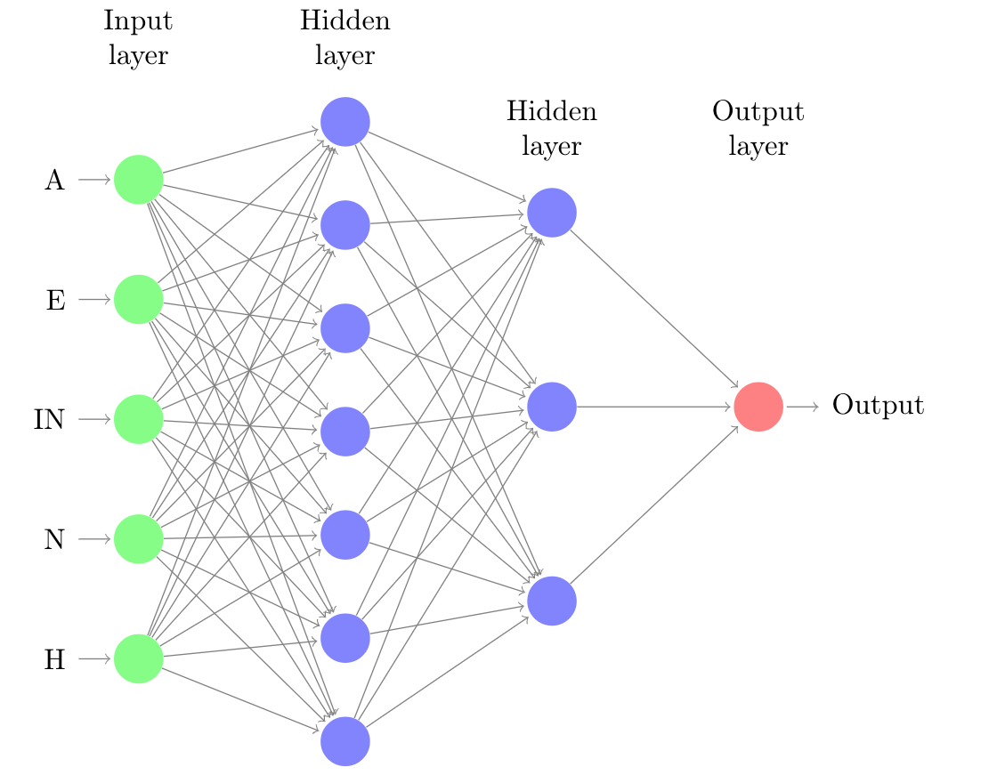
Figure 1: HOI network architecture. The input layer is comprised of five nodes, which is followed by two hidden layers of seven and three nodes, and an output layer of a single node.

A diagram showing the HOI architecture is presented in Fig. 1. The input layer is a vector of $five$ neurons that matches the dimensionality of the input, which is followed by two hidden layers that are composed of seven and three neurons, respectively, from the input layer. The output layer is composed of a single neuron whose values are restrained between 0 and 1 by virtue of the sigmoid function. Here, objects with a rating of 0.5 or above are classified as PI while those below the threshold are classified as UO. This neural network architecture was arrived at by a combination of empirical experimentation and the incorporation of domain knowledge. We wanted to provide the network with enough degrees of freedom to properly generalize the orbital elemental profiles of KI but to avoid giving it so many degrees of freedom that the network would overfit to the training datasets.

The described architecture results in 69 free parameters: 59 weights and ten biases . To optimize these parameters, the network is trained on five randomly selected sub-sets of 100,000 observed and KI objects over 20 epochs, which took less than five minutes on a CPU-type laptop without a GPU. The training was halted when the relative loss decrease per epoch was less than $1\%$ to prevent overfitting. At the end of the training process, the network’s performance was validated with a subset of 20,000 KI and 20,000 observed objects that had been held out of the training process. Furthermore, all potentially hazardous objects (PHOs) were held out of the training process and used exclusively for testing purposes. Fig. 2 shows how the training and validation loss decreased per training epoch, while the fraction of PHO hazardous objects identified simultaneously increased.

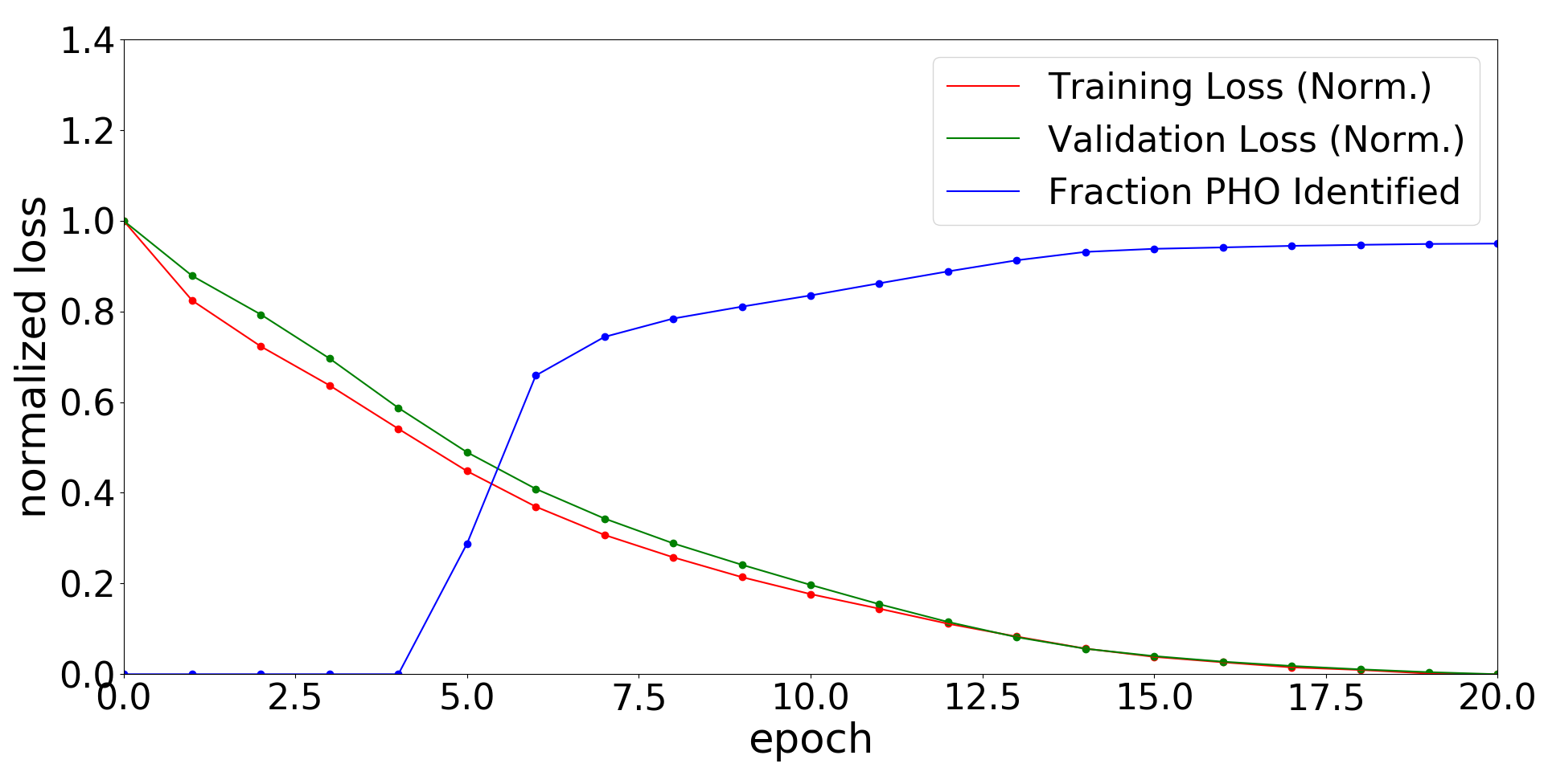
Figure 2: Normalized training and validation losses plotted against the training epoch number, along with the fraction of PHOs identified by the network.

We gave the observed objects and KIs labels of 0.1 and 0.9, respectively. Here, higher numbers correspond with a larger probability of colliding with Earth. The label of 0.9 was chosen for the KIs to represent calculations of the KI trajectories which are not converged solutions (Portegies Zwart & Boekholt 2014) and to show that several perturbing effects in the Solar System were neglected during the simulations, implying that all of the KIs will, in fact, not collide with Earth when their respective velocities are negated.

To arrive at the label of 0.1 for the observed objects, we assumed that any individual observed object is very likely to be benign by the following logic: first, all of the PHOs which have considerably larger probability to collide with the Earth compared with the rest of the observed population are not used in HOI training. As a result, their labeling does not degrade the network’s ultimate performance. Second, impacts from large objects are rare (Chapman & Morrison 1994) as the impact frequency of an asteroid collision decreases with the cube of an asteroid’s diameter. Earth collisions with 5 kilometer asteroids occur approximately every 20 million years, while those with a 100 meter asteroids occur every 500 years (Tedesco 1994). Because 98.4% of the observed objects used for our experiments are greater than 100 meters in diameter, we can use the following formula to estimate an upper-bound of the number of expected Earth impacts from asteroids in our sample within the next 20,000 years:

$$N_{collisions}=\int^{\infty}_{100}\frac{4\times 10^{7}}{D^{3}}=2000,$$ (3)

Where $D$ is the diameter of an asteroid. Given that over 700,000 objects were used in HOI training, the number of 2000 mislabeled objects implies that 0.3% of the observed labels are inaccurate. As discussed further in the following sections, although our sample contains only a small fraction of misclassified non-impactors, they still may effect the ability of HOI to accurately identify an impactor.

3 Data generation and acquisition

3.1 Observed objects

We extracted $736,496$ minor bodies from NASA’s dastcom5 database (Giorgini & Chamberlin 2014). A percentage of 95.5% of the extracted objects are main-belt asteroids, 3.2% are asteroids that are not in the main belt (such as Apollo or Trojan asteroids), 0.7% are comets, 0.2% are Kuiper-belt objects, and the remaining 0.4% is composed of a plethora of miscellaneous objects, such as planetary satellites and centaurs (Johnston 2018). These proportions, however, are not representative of the actual small-body populations because there is considerable observational bias towards the closer main-belt asteroids in comparison with more distant objects (Stern 2012).

3.2 Generating a database of known impactors

We generated an ensemble of 330,000 KIs according to Algorithm 1 to act as examples of hazardous objects. Here virtual objects are launched from future positions of Earth’s surface and then integrated backward in time to the present era. The idea is that the virtual objects’ trajectories would be similar to that of an asteroid observed in the present that would strike the Earth or come very close to it at some point in the future.

Algorithm 1 KI generation algorithm. Here, $T_{0}$ is the earliest Solar System orientation, $T_{1}$ is the latest orientation, $n$ is the number of KIs, and $\Delta T=(T_{1}-T-0)/n$

1:T=$[T_{0},T_{0}+\Delta t,T_{0}+2\Delta t,...,T_{0}+(n-1)\Delta t,T_{1}]$

2:for each $\tau$ in $T$ do

3:      Initialize the Solar System’s planets’ velocities and positions with values corresponding to epoch $\tau$.

4:      Launch a virtual object perpendicularly from Earth’s surface with a velocity magnitude randomly drawn from an even distribution between 15 and 45km/s.

5:      Integrate the object backward in time along with all other Solar System objects until the present epoch.

6:      If the object has left the Solar System or spun into the sun, discard it and rerun the simulation.

The future launch dates, defined by the orientation of the Solar System, are evenly distributed between 300 and 20,000 years in the future, which correspond to $T_{0}$ and $T_{1}$ values of 2318 and 22018, respectively. The launching velocities are selected to bracket the Earth’s and Solar System’s escape speeds of 11.2 and 42.5km/s, respectively. We deliberately did not attempt to mimic the observed asteroid impact velocities to allow the neural network to learn from the full range of parameters, rather than just based on a hand-selected subsample.

4 Results

4.1 Identifying Earth-impacting asteroids

The training of the network led to the positive identification of 95.25% of the KIs that were not part of the training and 90.99% of the PHOs as PIs. Additionally, 1.94% of the observed objects that were not classified as PHOs were identified as PIs. The high fraction of correctly identified KIs indicates that HOI positively recognizes most objects that are constructed to strike Earth. This result is not unexpected because HOI was specifically tuned to identify artificial KI objects. A more meaningful metric of performance is the percentage of PHOs identified. Although 9.01% PHOs were not classified as potential impactors, HOI is approximately 47 (90.99/1.94) times more likely to select a PHO over some other observed object.

To further evaluate the effectiveness of HOI, we performed simulations to compare the closest Earth approaches of PIs and UOs. To run these simulations, we began by loading the positions and velocities of the asteroids and other Solar System objects corresponding to January 1, 2018. We then integrated all of the bodies forward in time for a thousand years while saving the closest approach that the asteroids made relative to Earth. The trajectories of all the 14,680 observed PIs and an equal number of randomly selected UO asteroids were computed. The distributions of the closest Earth approaches achieved during these simulations are plotted in Fig. 3.

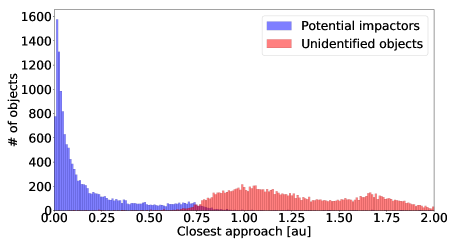
Figure 3: Closest approaches to Earth achieved in the next 1000 years for all the observed PIs and an equal number of randomly selected UOs. 108 PIs and 884 UOs are not plotted because their closest approaches exceeded the x-axis limits of 2  au. Every object that reach Earth within 0.01 au and 99.9% of objects within 0.05 au are identified by HOI as PIs.

To investigate why HOI only identified approximately nine-tenths of PHOs as PIs, the thousand-year integrations described above were additionally performed for all PHOs. We present in Fig.  4 the distributions of these closest approaches. The distributions of identified PHOs and unidentified PHOs are similar, therefore the fraction of PHOs identified as PIs could be used as a measure of the network’s performance. Additionally, all objects that did not approach Earth within at least 0.5 au could be considered misclassified PIs. This cut-off is not arbitrary but based, rather, on the minimum distance achieved by approximately 99.7%, or $3\sigma$, of PHOs. In the case of HOI, 12.2% of the PIs are outside of this threshold and are therefore considered misclassified. The root of this misclassification likely stems from the approximations made in the labeling schemes described in Section 2.

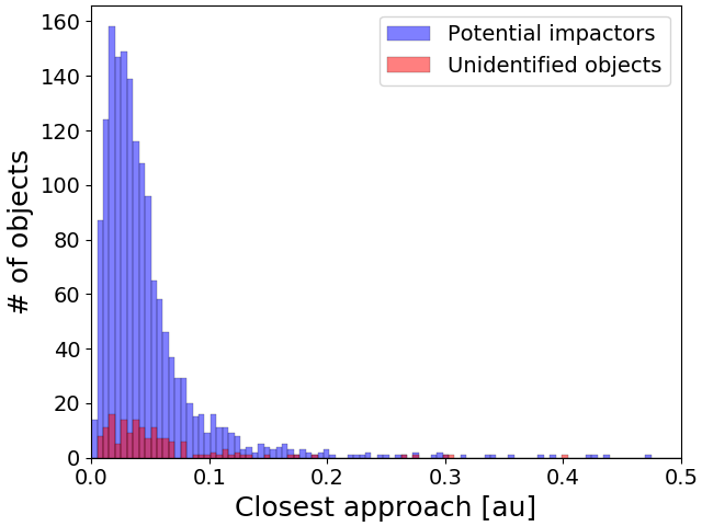
Figure 4: Closest approach distances to Earth reached for PHOs in the coming 1000 years.

A total of $13,258$ asteroids identified by HOI as KIs are not listed by NASA as PHOs. In our thousand-year integrations, $4472$ of these objects approached within 0.05 au of Earth while $2015$ approached within 0.02 au. In Table. 1 we present a short list of 11 notable asteroids with absolute magnitudes of less than 22, data arcs of less than 31 days, and closest approaches less than 0.02 au.

Designation	CA	$t_{\rm CA}$	H	arc
	[au]	[Year]	[mag]	[day]
2005 RV24	0.020	Feb. 2374	20.60	28
2008 UV99	0.013	April 2332	20.03	1
2011 BU10	0.006	April 2920	21.30	18
2011 HH1	0.012	July 2923	21.7	13
2011 WC44	0.018	Feb. 2679	20.5	31
2013 AG76	0.013	Dec. 2638	20.3	24
2014 GL35	0.018	July 2556	20.6	23
2014 TW57	0.017	Sept. 2165	20.1	24
2014 WD365	0.017	Sept. 2735	19.7	5
2017 DQ36	0.013	Dec. 2131	19.3	29
2017 JE3	0.016	July 2741	21.9	23

Table 1: Potential impactor shortlist: relatively large minor bodies with a short data arcs that were identified as PIs by HOI but are not considered PHOs. Along with their closest approaches (CA) in au, the month and year that their closest approaches occurred ($t_{\rm CA}$), their absolute magnitudes (H), and their data arc lengths in days (arc) are tabulated.

The absolute magnitude threshold of 22 was chosen so that only asteroids that have the potential of causing regional devastation unprecedented in human history would make the shortlist. Assuming a geometric albedo between 0.05 and 0.25 and a spherical shape, objects with an absolute magnitude of 22 are estimated to have diameters between from 100 m to 236 m. For perspective, Tunguska object which flattened 2,000 square kilometers of forest in Siberia was estimated to have a diameter of between 50-80 m (Farinella et al. 2001). The month long data-arc limit is selected because the Monte-Carlo method adopted by NASA is particularly ill-suited for calculating the impact probabilities of such uncertain orbits. As a consequence, these objects are the most likely to be overlooked as PHOs.

4.2 Comparing various populations of object

The characteristics of the simulated KIs and the observed objects are compared to better understand how HOI differentiates between the two populations. In Fig. 5 we present 100 trajectories of observed objects and KIs.

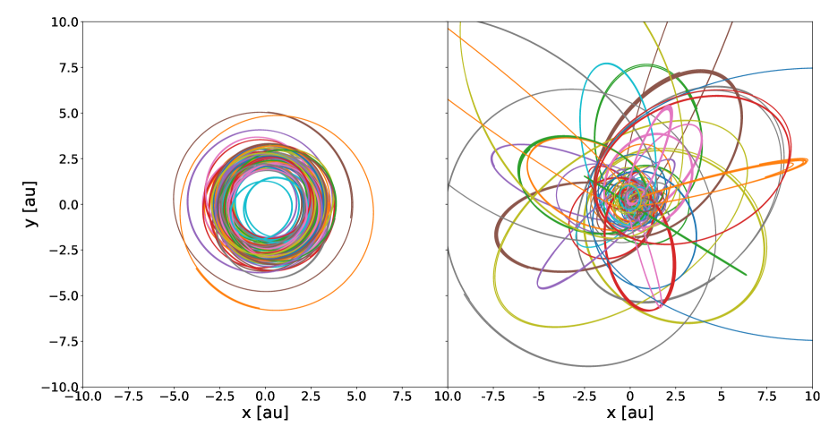
Figure 5: Illustration of the difference between the trajectories of observed objects (left) and KIs (right). The observed objects tend to have circular orbits which lie in the orbital plane of Earth around the Sun, whereas the KIs exhibit a much broader distribution in eccentricity and inclination. These characteristics, however, are not mutually exclusive and could be one the root causes of HOI’s imperfect classification.

There are profound differences between the orbital elements of the two distinct populations of objects. Our artificial population of objects launched from Earth tend to have highly eccentric and inclined orbits, whereas the observed objects tend to have circular orbits confined near the ecliptic plane. For the observed objects, the orbital plane is essentially empty within approximately 2 au of the Sun, while for the KIs this is the most densely occupied space. This object distribution should be expected considering that all the KIs were generated $1\pm 0.017$ au away from the Sun along the Earth’s orbit and that the integration times were not sufficiently long enough to allow considerable outward migration of the objects.

The a versus e ratio is an important factor in an object’s identification, as illustrated in Fig. 6. A curve is drawn to highlight an apparent “classification boundary”, which is above 95.2% of PI and below 90.3% of unidentified observed objects. Although the boundary is an indicator of an object’s potential classification, it is not definite, which is understandable considering that HOI takes five orbital elements as input for each object instead of just the a and e orbital elements.

5 Conclusions

We designed, constructed, and trained a fairly simple neural network aimed at classifying asteroids with the potential to impact the Earth over the coming $20,000$ years. Our method takes the observed orbital elements as input and provides a classifier for the expectation value for the object’s striking Earth.

The network was able pick out 95.25% of the KIs when mixed into a set of observed asteroids which are not expected to strike Earth. When applied to the entire population of observed asteroids, the network was able to identify approximately nine-tenths of the asteroids identified by NASA as PIs and along with virtually every other observed asteroid that approached within 0.05 au of Earth. We generated a short list of network identified PIs which NASA does not label as PHOs, mainly because the observed orbital elements are so uncertain that NASA’s Monte Carlo approach to determine their Earth-striking probability fails. The network classifies an object as a PI or UO within $0.25$ milliseconds, which is negligible compared to the time required for the Monte-Carlo method employed by NASA.

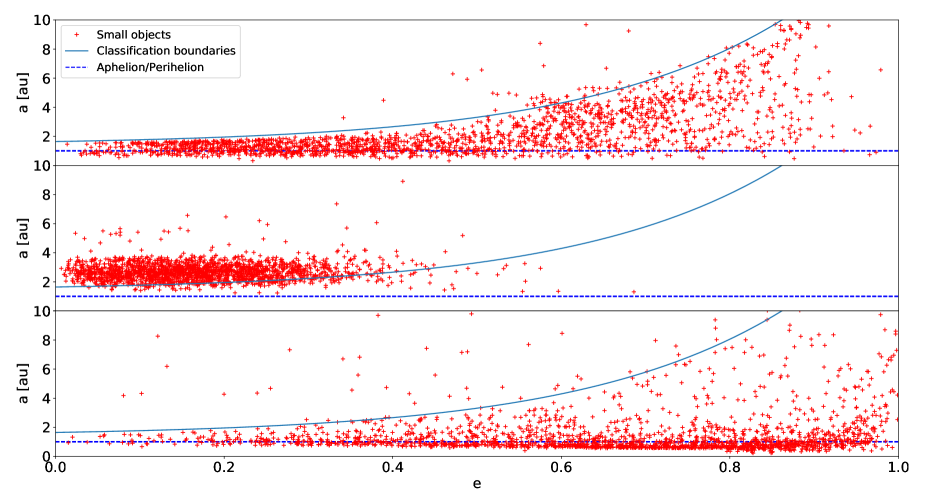
Figure 6: Plots the semi-major axis versus the eccentricity for 2,000 PI, UO and KI objects, respectively, from top to bottom. The dotted blue lines represent the aphelion and perihelion distances of Earth’s orbit and the teal curves represent the “classification boundary” where objects below are likely to be classified as PIs and those above are likely to be classified as benign.

Follow-up calculations over a time-span of 1000 years revealed that 12.2% of the PIs identified by the network did not come within 0.5 au of Earth. This may imply that thee asteroids pose no direct threat on the time scale considered. Integrating their orbits for a longer time-frame, however, this is impractical because of the large uncertainty in their orbital elements and the relatively small Lyapunov timescale for these objects.

We look forward to improving the network’s classification accuracy. The network, as we show in Fig. 1, is the result of a great deal of experimentation in network depth, width, and (sub)selection input parameters. It is possible that the structure preserving mimetic architectures motivated by the underlying Keplerian topology of the orbits could allow us to achieve a higher quality of prediction accuracy but this still requires a considerable degree of further experimentation. Another improvement could be carried out by considering a stricter labeling scheme in which some probability statistics for impacting the Earth could be taken into account.