Approximation smooth and sparse functions by deep neural networks without saturation

Abstract

Constructing neural networks for function approximation is a classical and longstanding topic in approximation theory. In this paper, we aim at constructing deep neural networks (deep nets for short) with three hidden layers to approximate smooth and sparse functions. In particular, we prove that the constructed deep nets can reach the optimal approximation rate in approximating both smooth and sparse functions with controllable magnitude of free parameters. Since the saturation that describes the bottleneck of approximate is an insurmountable problem of constructive neural networks, we also prove that deepening the neural network with only one more hidden layer can avoid the saturation. The obtained results underlie advantages of deep nets and provide theoretical explanations for deep learning.

1 Introduction

Machine learning [5] is a key sub-field of artificial intelligence (AI) which abounds in sciences, engineering, medicine, computational finance and so on. Neural network [29, 26, 16, 21] is an eternal topic of machine learning that makes machine learning no longer just like a machine to execute commands, but makes machine learning have the ability to draw inferences about other cases from one instance. Deep learning [12, 15] is a new active area of machine learning research based on deep structured learning model with appropriate algorithms, and is acclaimed as a magical approach to deal with massive data. Indeed, neural networks with more than one hidden layer are one of the most typical deep structured models in deep learning [12]. In current literature [21, 30], it was showed that deep nets outperform shallow neural networks (shallow nets for short) in the sense that deep nets break through some lower bounds for shallow nets. Furthermore, some studies [11, 18, 22, 27, 32, 33] have demonstrated the superiority of deep nets via showing that deep nets can approximate various functions while shallow nets fail with similar number of neurons.

Constructing neural networks to approximate continuous functions is a classical and prevalent topic in approximation theory. In 1996, Mhaskar [25] proved that neural networks with single hidden layer are capable of providing an optimal order of approximating smooth functions. The problem is, however, that the weights and biases of the constructrs shallow nets are huge, which usually leads to extremely large capacity [13]. Besides this partly positive approximation results, it was shown in [7, 22] that there is a bottleneck for shallow nets in approximating smooth functions in the sense that there is some lower bound for approximation. Moreover, Chui et al. [6] showed that shallow nets with an ideal sigmoidal activation function cannot provide localized approximation in Euclidean space. Furthermore, it was proved in [9] that shallow nets cannot capture the rotation-invariance property by showing the same approximate rates in approximating rotation-invariant function and general smooth function. All these results presented limitations of shallow nets from the approximation theory view point.

To overcome these limitations of shallow nets, Chui et al. [6] demonstrated that deep nets with two hidden layers can provide localized approximation. Further than that, Chui et al. [9] showed that deep nets with two hidden layers and controllable norms of weights can approximate the univariate smooth functions without saturation and adding depth can realize the rotation-invariance. Here, saturation [21] means that the approximation rate cannot be improved once the smoothness of functions achieves a certain level, which was proposed as an open question by Chen [2]. The general results by Lin [24] indicated that deep nets with two hidden layers and controllable weights possess both localized and sparse approximation properties in the spatial domain. They also proved that learning strategies based on deep nets can learn more functions with almost optimal learning rates than those based on shallow nets. The problem in [24] is that the saturation cannot be overcome. The above theoretical verifications demonstrate that deep nets with two hidden layers can really overcome some deficiency of shallow nets, but that is just partially.

Recent literature in deep nets [34, 17] proved that deep nets with ReLU activation function (denoting deep ReLU nets) are more efficiently in approximating smooth function and possess better generalization performance for numerous learning tasks than shallow nets. Nevertheless, the constructed deep ReLU nets are too deep, which results in several difficulty in training, including the gradient vanishing phenomenon and disvergence issue [12]. Furthermore, how to select the depth is still an open problem, and there is a common phenomenon that deep nets with huge hidden layers will lead to inoperable [15]. Under this circumstance, we hope to construct a deep net with good approximation capability, controllable parameters, non-saturation and not too deep. To this end, we construct in this paper a deep net with three hidden layers that possesses the following properties: localized approximation, optimal approximation rate, controllable parameters, non-saturation and spatial sparsity. Our main tool for analysis is the localized approximation [7, 24], “product gate” strategy [9, 31, 34] and localized Taylor polynomials [17, 31].

2 Main results

Let $I=[0,1]$, $d\in\mathbb{N}$, $x\in X:=I^{d}$, $C(\mathbb{R}^{d})$ be the space of continuous functions with the norm

$$\|f\|_{\infty}:=\|f\|_{C(\mathbb{R}^{d})}:=\max_{x\in{\mathbb{R}^{d}}}|f(x)|.$$

For $x\in X$, the set of shallow nets can be mathematically expressed as

$$F_{\sigma,n}(x)=\left\{\sum_{i=1}^{n_{0}}c_{i}\sigma(w_{i}\cdot x+b_{i}):w_{i}\in\mathbb{R}^{d},b_{i},c_{i}\in\mathbb{R}\right\}$$ (2.1)

where $\sigma:\mathbb{R}\rightarrow\mathbb{R}$ is an activation function, $n_{0}$ is the number of hidden neurons (nodes), $c_{i}\in\mathbb{R}$ is the outer weights, $w_{i}:=(w_{ji})_{j=1}^{d}\in\mathbb{R}^{d}$ is the inner weight, and $b_{i}$ is the bias (threshold) of the $i$-$th$ hidden nodes.

Let $l\in\mathbb{N}$, $d_{0}=d,d_{1},\cdots,d_{l}\in\mathbb{N}$, $\sigma_{k}:\mathbb{R}\rightarrow\mathbb{R}~{}(k=1,2,\cdots,l)$ be univariate nonlinear functions. For $\vec{h}=(h^{(1)},\cdots,h^{(d_{k})})^{T}\in\mathbb{R}^{d_{k}}$, define $\vec{\sigma}(\vec{h})=(\vec{\sigma}(h^{(1)}),\cdots,\vec{\sigma}(h^{(d_{k})}))^{T}$. Denote $\mathcal{H}_{\{\sigma_{j},l,\tilde{n}\}}$ as the set of deep nets with $l$ hidden layers and $\tilde{n}$ free parameters that can be mathematically represented by

$$h_{\{\sigma_{j},l,\tilde{n}\}}(x)=\vec{a}\cdot\vec{h}_{l}(x)$$ (2.2)

where

$$\vec{h}_{k}(x)=\vec{\sigma}_{k}(W_{k}\cdot\vec{h}_{k-1}(x)+\vec{b}_{k}),~{}k=1,2,\cdots,l,$$

$h_{0}(x)=x,\vec{a}\in\mathbb{R}^{d_{l}},\vec{b}_{k}\in\mathbb{R}^{d_{k}}$, $W_{k}:=(W_{i,j}^{k})_{d_{k}\times d_{k-1}}$ is a $d_{k}\times d_{k-1}$ matrix, and $\tilde{n}$ denotes the number of free parameters, i.e., $\tilde{n}=\sum_{k=1}^{l}(d_{k}\cdot d_{k-1}+d_{k})+d_{l}$. The structure of deep nets, depicted in Figure 1, depends mainly on the structures of the weight matrices $W_{k}$ and the parameter vectors $\vec{b}_{k}$ and $\vec{a}$, $k=1,2,\cdots,l$. It is easy to see that when $l=1$, the function defined by (2.2) is a shallow net.

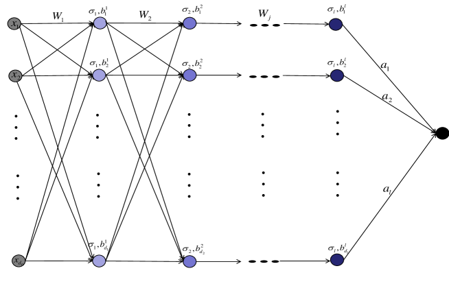
Figure 1: Structure for deep neural networks

2.1 Approximation of smooth function by Deep Nets

In this part, we focus on approximating smooth functions by deep nets. The smooth property is a widely used priori-assumption in approximation and learning theory [8, 10, 14, 23, 34]. Let $c_{0}$ be a positive constant, $r=k+v$ with $k\in\mathbb{N}_{0}:=\{0\}\bigcup\mathbb{N}$ and $0<v\leq 1$. A function $f:X\rightarrow\mathbb{R}$ is said to be $(r,c_{0})$-smooth if $f$ is $k$-times differentiable and for any $\alpha_{j}\in\mathbb{N}_{0},j=1,\cdots,d$ with $\alpha_{1}+\cdots+\alpha_{d}=k$, then for any $x,z\in X$, the partial derivatives $\partial^{k}f/{\partial x_{1}^{\alpha_{1}}\cdots\partial x_{d}^{\alpha_{d}}}$ exist and satisfy

$$\left|\frac{\partial^{k}f}{\partial x_{1}^{\alpha_{1}}\cdots\partial x_{d}^{\alpha_{d}}}(x)-\frac{\partial^{k}f}{\partial x_{1}^{\alpha_{1}}\cdots\partial x_{d}^{\alpha_{d}}}(z)\right|\leq c_{0}\|x-z\|^{v}.$$ (2.3)

Throughtout this paper, $\|x\|$ denotes the Euclidean norm of $x$. In particular, if $0<r\leq 1$, then (2.3) coincides the well known Lipschitz condition:

$$|f(x)-f(z)|\leq c_{0}\|x-z\|^{r},\forall x,z\in X.$$ (2.4)

Denote by $Lip(r,c_{0})$ be the family of $(r,c_{0})$-Lipschitz functions satisfying (2.4). In fact, the Lipschitz property depicts the smooth information of $f$ and has been adopted in huge literature [30, 6, 9, 24, 20] to quantify the approximation ability of neural networks.

As we know, different activation functions used in neural networks will lead to different results [30]. Among all the activation functions, the sigmoidal function and Heaviside function are two commonly used ones. Similar as [24], we use these two activation functions to construct deep nets. The main reason is that the usage of Heaviside function can enhance the localized approximation performance [24] and the adoption of sigmoidal function can improve the capability to approximate algebraic polynomials [9]. Let $\sigma_{0}$ be the Heaviside function, i.e.,

$$\sigma_{0}(t)=1,\mbox{if~{}}t\geq 0;~{}\sigma_{0}(t)=0,\mbox{if~{}}t<0,$$

and $\sigma:\mathbb{R}\rightarrow\mathbb{R}$ be a sigmoidal function, i.e.,

$$\lim_{t\rightarrow+\infty}\sigma(t)=1,\lim_{t\rightarrow-\infty}\sigma(t)=0.$$ (2.5)

Due to (2.5), for any $\varepsilon>0$, there exists a $K_{\varepsilon}=K(\varepsilon,\sigma)>0$ such that

$$\left\{\begin{array}[]{cc}|\sigma(t)-1|<\varepsilon,\mbox{~{}if~{}}t\geq K_{\varepsilon},\\ |\sigma(t)|<\varepsilon,\mbox{~{}~{}if~{}}t\leq-K_{\varepsilon}.\end{array}\right.$$ (2.8)

Before presenting the main results, we should introduce some assumptions. Assumption 1 is the $r$-Lipschitz continuous condition for the target function, which is a standard condition in approximation and learning theory.

Assumption 1 We assume $g\in\mbox{Lip}(r,c_{0})$ with $r=k+v$, $k\in\mathbb{N}_{0}$, $0<v\leq 1$, $c_{0}>0$.

Assumption 2 concerns the smoothness condition on activation function $\sigma$, which has already been adopted in [19].

Assumption 2 For $r>0$ with $r=k+v$, $k\in\mathbb{N}_{0}$, $0<v\leq 1$, let $\sigma$ be a non-decreasing sigmoidal function with $\|\sigma^{\prime}\|_{L_{\infty}(R)}\leq 1$, $\|\sigma\|_{L_{\infty}(R)}\leq 1$ and there exists at least a point $b_{0}\in\mathbb{R}^{d}$ satisfies $\sigma^{(j)}(b_{0})\neq 0$ for all $j=0,1,2,\cdots,k_{0}$, and $k_{0}\geq\max\{k,2\}+1$.

There are many functions satisfy the above restrictions such as: the Logistic function $\sigma(t)=\frac{1}{1+e^{-t}}$, the Hyperbolic tangent function $\sigma(t)=\frac{1}{2}(\tanh(t)+1)$, the Gompertz function $\sigma(t)=e^{-ae^{-bt}}$ with $a,b>0$ and the Gaussian function $\sigma(t)=e^{-t^{2}}$.

Our first main result is the following theorem, in which we construct a deep net with three hidden layers to approximate smooth functions. Denote by $\mathcal{H}_{3,\tilde{n}}:=\mathcal{H}_{\{\sigma_{0},\sigma,\sigma,3,\tilde{n}\}}$ be the set of deep net with three hidden layers and $\tilde{n}$ free parameters, where $\sigma_{0},\sigma,\sigma$ are the activation functions in the first, second and third hidden layers, respectively.

Theorem 2.1

Let $0<\varepsilon\leq 1$, under Assumptions 1 and 2, there exists a deep net $H(x)\in\mathcal{H}_{\{3,\tilde{n}\}}$ such that

$$|g(x)-H(x)|\leq C(\tilde{n}^{-\frac{r}{d}}+\tilde{n}\varepsilon),$$ (2.9)

where all parameters of this deep net are bounded by $\mbox{poly}(\tilde{n},\frac{1}{\varepsilon})$, $\mbox{poly}(\tilde{n},\frac{1}{\varepsilon})$ denotes some polynomial function with respect to $\tilde{n}$ and $\frac{1}{\varepsilon}$, and $C$ is a constant independent of $\tilde{n}$ and $\varepsilon$.

The proof of Theorem 2.1 will be postponed in Section 4, and a direct consequences of Theorem 2.1 is as follows.

Corollary 2.2

Under Assumptions 1 and 2, if $\varepsilon=\tilde{n}^{-\frac{r+d}{d}}$, then there holds

$$|g(x)-H(x)|\leq\bar{C}\tilde{n}^{-\frac{r}{d}},$$ (2.10)

where $\bar{C}$ is a constant independent of $\tilde{n}$, and all the parameters of the deep net are bounded by $\mbox{poly}(\tilde{n})$.

The approximation rate of shallow nets and deep nets with two hidden layers are $\mathcal{O}(\tilde{n}^{-\frac{r}{d}})$ [29, 9], which is the same as Corollary 2.2. However, as far as the norm of weights is considered, all the weights in Corollary 2.2 are controllable, and are much less than those of shallow nets. Specifically, for shallow nets, the norm of weights is at least exponential with respect to $\tilde{n}$ [25], while for deep nets in Corollary 2.2, the norm of weights is only polynomial respect to $\tilde{n}$. Such a difference is essentially according to the capacity estimate [13], where a rigorous proof was presented that the covering number of deep nets with controllable norms of free parameters can be tightly bounded. Furthermore, compared with similar results for deep nets with two hidden layers [24], we find that our constructed deep net avoids the saturation. To sum up, the constructed deep net with three hidden layers performs better than shallow nets and deep nets with two hidden layers in overcoming their shortcomings.

2.2 Sparse Approximation for Deep Nets

Sparseness in the spatial domain is a prevalent data feature that abounds in numerous applications such as magnetic resonance imaging (MRI) analysis [1], handwritten digit recognition [4] and so on. The spatial sparseness means that the response (or function) of some actions only happens on several small regions instead of the whole input space. In other words, the response vanishes in most of regions of the input space. Mathematically, the spatially sparse function is defined as follows [24].

Let $s,N\in\mathbb{N}$, $s\leq N^{d}$, $N_{N}^{d}=\{1,2,...,N\}^{d}$. Denote by $\{B_{N,\jmath}\}_{\jmath\in N_{N}^{d}}$ a cubic partition of $I^{d}$ with centers $\{\zeta_{\jmath}\}_{\jmath\in N_{N}^{d}}$ and side length $\frac{1}{N}$. Define

$$\Lambda_{s}:=\{\mathbf{k}_{\ell}:\mathbf{k}_{\ell}\in N_{N}^{d},1\leq{\ell}\leq s\}$$

and

$$S:=\bigcup_{\jmath\in\Lambda_{s}}B_{N,\jmath}.$$

For any function $f$ defined on $I^{d}$, if the support of $f$ is $S$, then we say that $f$ is $s$-sparse in $N^{d}$ partitions. We use $Lip(N,s,r,c_{0})$ to quantify both the smoothness property and sparseness, i.e.,

$$Lip(N,s,r,c_{0})=\left\{f:f\in Lip(r,c_{0})~{}\mbox{and}~{}f~{}\mbox{is s-sparse in}~{}N^{d}~{}\mbox{partition}\right\}.$$

For $n\in\mathbb{N}$ with $n\geq\hat{c}N$ for some $\hat{c}>0$, let $\{A_{n,j}\}_{j\in\mathbb{N}_{n}^{d}}$ be another cubic partition of $I^{d}$ with centers $\{\xi_{j}\}_{j\in\mathbb{N}_{n}^{d}}$ and side length $\frac{1}{n}$. For each $\jmath\in\mathbb{N}_{N}^{d}$, define

$$\bar{\Lambda}_{\jmath}:=\{j\in N_{n}^{d}:A_{n,j}\cap B_{N,\jmath}\neq\emptyset\},$$

it is easy to see that the set $\bigcup_{\jmath\in\bigwedge_{s}}\bar{\Lambda}_{\jmath}$ is the family of $A_{n,j}$ where $f$ is not vanished.

With these helps, we present a spareness assumption of $f$ as follows.

Assumption 3 We assume $f\in\mbox{Lip}(N,s,r,c_{0})$ with $r=k+v$, $k\in\mathbb{N}_{0}$, $0<v\leq 1$, $c_{0}>0$, $N,s\in\mathbb{N}$.

In [9], Chui et al. only discussed the approximating performance of deep nets with two hidden layers in approximating smooth function. Lin [24] extended the results in [9] to approximate spatially sparse functions. Specifically, Lin [24] proved that deep nets with two hidden layers can approximate spatially sparse function much better than shallow nets. However, their results suffered from the saturation. In this subsection, we aim at conquering the above deficiency by constructing a deep net with three hidden layers. Theorem 2.3 below is the second main result of this paper, and the proof also be verified in Section 4.

Theorem 2.3

Let $0<\varepsilon\leq 1$, $\tilde{n}\geq\tilde{c}N^{d}$ for some $\tilde{c}>0$. Under Assumptions 2 and 3, there exists a deep net $H(x)\in\mathcal{H}_{\{3,\tilde{n}\}}$ such that

$$|f(x)-H(x)|\leq c_{0}\tilde{n}^{-\frac{r}{d}}+\tilde{C}\tilde{n}\varepsilon,~{}\forall x\in X.$$

If $x\in{I^{d}}\setminus\bigcup_{\jmath\in\Lambda_{s}}\bar{\Lambda}_{\jmath}$, then

$$|H(x)|\leq\tilde{C}\tilde{n}\varepsilon$$

where all the parameters of the deep net are bounded by $\mbox{poly}(\tilde{n},\frac{1}{\varepsilon})$, and $\tilde{C}$ is a constant independent of $\tilde{n}$ and $\varepsilon$.

Corollary 2.4

Let $T$ be arbitrary positive number satisfies $T\geq\frac{r+d}{d}$ and $\varepsilon=\tilde{n}^{-T}$. Under the Assumptions 2 and 3, if $\tilde{n}\geq\tilde{c}N^{d}$ for some $\tilde{c}>0$, then there holds

$$|f(x)-H(x)|\leq\hat{C}\tilde{n}^{-\frac{r}{d}},~{}\forall x\in X.$$ (2.11)

If $x\in X\setminus\bigcup_{\jmath\in\Lambda_{s}}\bar{\Lambda}_{\jmath}$, then

$$|H(x)|\leq\tilde{n}^{-T}$$ (2.12)

where $\hat{C}$ is a constant independent of $\tilde{n}$.

To be detailed, (2.11) shows that the approximation rate of deep nets is as fast as $\mathcal{O}(\tilde{n}^{-\frac{r}{d}})$, and (2.12) states their performance in realizing the spatial sparseness, when $T$ is large. However, too large $T$ may lead to extremely large weights, which implies huge capacity measured by the covering number of $\mathcal{H}_{\{3,\tilde{n}\}}$ according to [13]. A preferable choice of $T$ should be $T=\mathcal{O}(\frac{r+d}{d})$.

Previous studies [3, 6] indicated that shallow nets cannot provide localized approximation, which is a special case for sparse approximation with $s=1$. Lemma 4.1 (in Section 4) shows that deep nets with two hidden layers have the localized approximation property, which is the building-block to construct deep nets possessing sparse approximation property. To the best our knowledge, [24] is the first work to construct deep nets to realize sparse features. Compared with [24], our main novelty is to deepen the network to conquer the saturation.

3 Related work

Constructing neural networks to approximate the functions is a classic problem [29, 25, 27, 31, 10, 14, 24] in approximation theory. Traditional method to deal with this problem can be divided into three steps. Step 1, constructing a neural network to approximate polynomials; Step 2, utilizing polynomials to approximate target functions; Step 3, combining the above two steps to reach the final approximation results between neural networks and target functions. Tayor formula is usually be used in Step 1 to obtain the approximation results, which usually leads to extremely large weights, i.e., $|w_{i}|\sim e^{m}$, where $m$ is the degree of the polynomial. However, larger weight leads to large capability and consequently bad generalization and instable algorithms. Typical example includes [25] and [28]. In order to overcome this drawback, we introduce a new function by the product of Taylor polynomial and a deep net with two hidden layers to instead of the polynomial in Step 1 to reduce the weights of neural networks from $e^{m}$ to $\mbox{poly}(m)$.

For deep nets, [34] and [31] stated that deep ReLU networks are more efficient to approximate smooth functions than shallow nets. But their results are slightly worse than Theorem 2.1 in this paper, in the sense that there is either an additional logarithmic term or under the weaker norm. Recently, Han et al. [17] indicated that deep ReLU nets can achieve the optimal generalization performance for numerous learning tasks, but the depth of [31] is much larger than ours. Recently, Zhou [35, 36] also verified that deep convolutional neural network (DCNN) is universal, i.e., DCNN can be used to approximate any continuous function to an arbitrary accuracy when the depth of the neural network is large enough.

All the above literature [34, 31, 17, 35, 36] demonstrated that deep nets with ReLU activation function and DCNN have good properties both in approximation and generalization. However, there are too deep to be particularly used in real tasks. Compared with these results, we constructed a deep net only with three hidden layers to approximate smooth and sparse functions, respectively. We proved in Theorem 2.1 and Theorem 2.3 that the constructed deep net with three hidden layers and with controllable weights, can realize smoothness and spatial sparseness without saturation, simultaneously.

4 Proofs

Let $\mathcal{P}_{m}=\mathcal{P}_{m}(\mathbb{R}^{d})$ be the set of multivariate algebraical polynomials on $\mathbb{R}^{d}$ of degree at most $m$, i.e.,

$${\mathcal{P}}_{m}=span\{x^{k}\equiv x_{1}^{k_{1}}\cdots x_{d}^{k_{d}}:|k|=k_{1}+...+k_{d}\leq m\}.$$

Consider $\mathcal{P}_{m}^{h}$ as the set of homogeneous polynomials of degree $m$, i.e.,

$$\mathcal{P}_{m}^{h}=span\{x^{k}=x_{1}^{k_{1}}\cdots x_{d}^{k_{d}}:|k|=k_{1}+...+k_{d}=m\}.$$

4.1 Localized Approximation for Deep Nets

Let $\mathbb{N}_{n}^{d}=\{1,2,\cdots,n\}^{d}$, $n\in\mathbb{N}$, $\{A_{n,j}\}_{j\in\mathbb{N}_{n}^{d}}$ be the cubic partition of $X$ with centers $\{\xi_{j}\}_{j\in\mathbb{N}_{n}^{d}}$ and side length $\frac{1}{n}$. If $x$ lies on the boundary of some $A_{n,j}$, then $j_{x}$ is the set to be the smallest integer satisfying $x\in A_{n,j}$, i.e.,

$$j_{x}=\left\{j|j\in N_{n}^{d},x\in A_{n,j}\right\}.$$

Then, for $K>0$, any $j\in\mathbb{N}_{n}^{d}$, $x\in X$, we construct a deep net with two hidden-layer $N^{*}_{n,j,K}(x)\in\mathcal{H}_{\{\sigma_{0},\sigma,2,2d+1\}}$ as

$$N^{*}_{n,j,K}(x)=\sigma\left\{2K\left[\sum_{l=1}^{d}\sigma_{0}\left[\frac{1}{2n}+x^{(l)}-\xi_{j}^{(l)}\right]+\sum_{l=1}^{d}\sigma_{0}\left[\frac{1}{2n}-x^{(l)}+\xi_{j}^{(l)}\right]-2d+\frac{1}{2}\right]\right\}.$$

Localized approximation of neural networks [6] implies that if the target function is modified only on a small subset of the Euclidean space, then only a few neurons, rather than the entire network, need to be retrained. Lemma 4.1 below that was proved in [24] states the localized approximation property of deep nets which is totally different from the shallow nets. We refer [9] (section 3.3) for details in the localized approximation of neural networks.

Lemma 4.1

For any $\varepsilon>0$, if $N^{*}_{n,j,K_{\varepsilon}}$ is defined by (4.1) with $K_{\varepsilon}$ satisfying (2.8) and $\sigma$ being a nondecreasing sigmoidal function, then

(i) For any $x\not\in A_{n,j}$, there holds $|N^{*}_{n,j,K_{\varepsilon}}(x)|<\varepsilon$;

(ii) For any $x\in A_{n,j}$, there holds $|1-N^{*}_{n,j,K_{\varepsilon}}(x)|\leq\varepsilon$.

It is easy to see that if $\varepsilon\rightarrow 0$, then $N^{*}_{n,j,K_{\varepsilon}}$ is an indicator function for $A_{n,j}$. Moreover, when $n\rightarrow\infty$, it indicates that $N^{*}_{n,j,K_{\varepsilon}}$ can recognize the location of $x$ in an arbitrarily small region and will vanish in some of partitions of the input space.

In order to overcome the deficiency of traditional method in neural networks approximation. We defined a new function $\Phi_{g}(x)$ by a product of Taylor polynomial and a deep network function with two hidden layers to instead of polynomials:

$$\Phi_{g}(x)=\sum_{j\in\mathbb{N}_{n}^{d}}P_{k,\eta_{j},g}(x)N^{*}_{n,j,K_{\varepsilon}}(x),~{}x\in X,$$ (4.2)

where $N^{*}_{n,j,K_{\varepsilon}}$ and $K_{\varepsilon}$ are defined by (4.1) and (2.8). $P_{k,\eta_{j},g}(x)$ is the Taylor polynomial of $g$ with degree $k$ around $\eta_{j}$, $\eta_{j}\in A_{n,j}$ and $j\in N_{n}^{d}$.

Based on the localized approximation results and the localized Taylor polynomial in (4.2), we construct a deep net with three hidden layers to approximate both smooth and sparse functions.

4.2 Proof of Theorem 2.1

The following proposition indicates that constructing a shallow net with one neuron can replace a minimal.

Proposition 4.2

Let $c_{0}>0,L=\mathcal{O}(m^{d-1})$, $\sigma\in Lip(r_{0},c_{0})$ is a sigmoidal function with $(m+1)-$times bounded derivatives, and $\parallel{\sigma}^{\prime}\parallel_{L_{\infty}(\mathbb{R})}\leq 1$, $\sigma^{(j)}(0)\neq 0$ for all $j=0,1,...,s_{0}$. For arbitrary $P_{m}\in\mathcal{P}_{m}$ and any $\varepsilon\in(0,1)$, we have

$$\left|P_{m}(x)-\sum_{i=1}^{L}\frac{C(i,m)m!}{\delta_{m}^{m}\sigma^{(m)}(0)}\sigma(\delta_{m}(w_{i}\cdot x))-P^{*}_{m-1}(x)\right|<\varepsilon.$$ (4.3)

where

$$P_{m-1}^{*}(x)=\sum_{j=0}^{m-1}\sum_{i=1}^{L}D(i,j)(w_{i}\cdot x)^{j},~{}D(i,j)=C(i,j)-\frac{C(i,m)m!\sigma^{(j)}(0)}{\delta_{m}^{m}\sigma^{(m)}(0)j!},$$

$$\delta_{m}=\min\left\{\frac{\varepsilon}{M_{m}},\frac{\varepsilon}{\sum_{i=1}^{L}|C(i,m)|M_{m}}\right\},~{}M_{m}=\max_{-1\leq\xi\leq 1}\frac{\sigma^{(m+1)}(\xi)}{\sigma^{(m)}(0)},$$

and $C(i,j)$ is an absolute constant.

We use the Taylor formula [9] to prove the above Proposition 4.2.

Lemma 4.3

Let $k\geq 1$ and $\varphi$ be $k-$times differentiable on ${\mathbb{R}}$. Then for any $u,u_{0}\in{\mathbb{R}}$, there holds

$$\varphi(u)=\varphi(x_{0})+\frac{\varphi^{{}^{\prime}}(u_{0})}{1!}(u-u_{0})+...+\frac{\varphi^{k}(u_{0})}{k!}(u-u_{0})^{k}+R_{k}(u)$$ (4.4)

where

$$R_{k}(u)=\frac{1}{(k-1)!}\int_{u_{0}}^{u}[\varphi^{(k)}(t)-\varphi^{(k)}(u_{0})](u-t)^{k-1}dt.$$ (4.5)

In addition, under the condition of Lemma 4.3, for any $a\in{\mathbb{R}}$, there holds

$$\varphi(au)=\varphi(u_{0})+\frac{\varphi^{{}^{\prime}}(u_{0})}{1!}(au-u_{0})+...+\frac{\varphi^{k}(u_{0})}{k!}(au-u_{0})^{k}+R_{k}(u)$$ (4.6)

where

$$R_{k}(u)=\frac{a^{k}}{(k-1)!}\int_{u_{0}}^{u}[\varphi^{k}(at)-\varphi^{k}(u_{0})](u-t)^{k-1}dt.$$ (4.7)

Lemma 4.4 which was proved in [28] plays an important role in proving Proposition 4.2.

Lemma 4.4

Let $m\in\mathbb{N}$ and $L=\mathcal{O}(m^{d-1})$. For any $P_{m}\in{\mathcal{P}}_{m}$, there exists a set of points $\{w_{1},...,w_{L}\}\subset I^{d}$ such that

$$P_{m}(x)=span\{(w_{i}\cdot x)^{j}:x,w_{i}\in I^{d},0\leq j\leq m,1\leq i\leq L\}.$$ (4.8)

Proof of Proposition 4.2. For any $t\in[0,1]$, ${\delta_{k}}\in(0,1)$, $k\in[1,s_{0}]$, it follows from Lemma 4.3 that

$$\sigma({\delta_{k}}t)=\sigma(0)+\frac{\sigma^{{}^{\prime}}(0)}{1!}{\delta_{k}}t+...+\frac{\sigma^{k}(0)}{k!}({\delta_{k}}t)^{k}+\tilde{R}_{k}(t)$$ (4.9)

where

$$\tilde{R}_{k}(t)=\frac{\delta_{k}^{k}}{(k-1)!}\int_{0}^{t}[\sigma^{(k)}({\delta_{k}}u)-\sigma^{(k)}(0)](t-u)^{k-1}du.$$ (4.10)

Denote

$$Q_{k-1}(t)=\sum_{j=0}^{k-1}\frac{\sigma^{(j)}(0)}{j!}({\delta_{k}}t)^{j}.$$

Then (4.9) yields

$$t^{k}=\frac{k!}{\delta_{k}^{k}\sigma^{(k)}(0)}\sigma({\delta_{k}}t)-\frac{k!}{\delta_{k}^{k}\sigma^{(k)}(0)}Q_{k-1}(t)-\frac{k!}{\delta_{k}^{k}\sigma^{(k)}(0)}\tilde{R}_{k}(t),$$

which implies

$$t^{k}=\frac{k!}{\delta_{k}^{k}\sigma^{(k)}(0)}\sigma({\delta_{k}}t)+q_{k-1}(t)+r_{k}(t)$$ (4.11)

where

$$q_{k-1}(t)=-\frac{k!}{\delta_{k}^{k}\sigma^{(k)}(0)}Q_{k-1}(t)$$

and

$$r_{k}(t)=-\frac{k!}{\delta_{k}^{k}\sigma^{(k)}(0)}\tilde{R}_{k}(t).$$ (4.12)

Since

$$|\sigma^{(k)}({{\delta_{k}}}u)-\sigma^{(k)}(0)|\leq\max_{0<\xi<1}|\sigma^{(k+1)}(\xi)||{\delta_{k}}||u|,$$

then by (4.10) and (4.12), there holds

$$|r_{k}(t)| = \left|-\frac{k!}{\delta_{k}^{k}\sigma^{(k)}(0)}\tilde{R}_{k}(t)\right|$$ (4.13)

$$= \frac{k}{|\sigma^{(k)}(0)|}\left|\int_{0}^{t}[\sigma^{(k)}({\delta_{k}}u)-\sigma^{(k)}(0)](t-u)^{k-1}du\right|$$

$$\leq \frac{k|\sigma^{(k+1)}(\xi)|}{|\sigma^{(k)}(0)|}\left|\int_{0}^{t}{\delta_{k}}u(t-u)^{k-1}du\right|=\frac{{\delta_{k}}k|\sigma^{(k+1)}(\xi)|}{|\sigma^{(k)}(0)|}\left|\int_{0}^{1}u(1-u)^{k-1}du\right|$$

$$\leq k{\delta_{k}}M_{k}(\frac{1}{k}-\frac{1}{1+k})\leq{\delta_{k}}M_{k}.$$

From Lemma 4.4, for any $P_{m}\in\mathcal{P}_{m}$, it follows

$$P_{m}(x) = \sum_{j=0}^{m}\sum_{i=1}^{L}C(i,j)(w_{i}\cdot x)^{j}$$ (4.14)

$$= \sum_{i=1}^{L}C(i,m)(w_{i}\cdot x)^{m}+\sum_{i=1}^{L}C(i,m-1)(w_{i}\cdot x)^{m-1}$$

$$+\cdots+\sum_{i=1}^{L}C(i,1)(w_{i}\cdot x)+\sum_{i=1}^{L}C(i,0).$$

Since $x,w_{i}\in I^{d}$, we have $|w_{i}\cdot x|\leq 1$. Then, for an arbitrary $\varepsilon>0$, there exists a $\delta_{m}\in(0,1)$ such that

$$\sum_{i=1}^{L}|C(i,m)|M_{m}\delta_{m}\leq\varepsilon.$$ (4.15)

Due to (4.11) and $\delta_{m}|w_{i}\cdot x|\in[0,1]$, there holds

$$(w_{i}\cdot x)^{m}=\frac{m!}{\delta_{m}^{m}\sigma^{(m)}(0)}\sigma(\delta_{m}(w_{i}\cdot x))+q_{m-1}(w_{i}\cdot x)+r_{m}(w_{i}\cdot x).$$ (4.16)

Inserting the above (4.16) into (4.14), we obtain

$$P_{m}(x) = \sum_{i=1}^{L}C(i,m)\left(\frac{m!}{\delta_{m}^{m}\sigma^{(m)}(0)}\sigma(\delta_{m}(w_{i}\cdot x))+q_{m-1}(w_{i}\cdot x)+r_{m}(w_{i}\cdot x)\right)$$ (4.17)

$$+\sum_{i=1}^{L}C(i,m-1)(w_{i}\cdot x)^{m-1}+\cdots+\sum_{i=1}^{L}C(i,1)(w_{i}\cdot x)+\sum_{i=1}^{L}C(i,0)$$

$$= \sum_{i=1}^{L}C(i,m)\frac{m!}{\delta_{m}^{m}\sigma^{(m)}(0)}\sigma(\delta_{m}(w_{i}\cdot x))+P_{m-1}^{*}(x)+R_{m}(x)$$

where

$$R_{m}(x)=\sum_{i=1}^{L}C(i,m)r_{m}(w_{i}\cdot x)$$

and

$$P_{m-1}^{*}(x) = \sum_{i=1}^{L}C(i,m)q_{m-1}(w_{i}\cdot x)+\sum_{i=1}^{L}C(i,m-1)(w_{i}\cdot x)^{m-1}$$ (4.18)

$$+\cdots+\sum_{i=1}^{L}C(i,1)(w_{i}\cdot x)+\sum_{i=1}^{L}C(i,0)$$

$$= \sum_{i=1}^{L}D(i,m-1)(w_{i}\cdot x)^{m-1}+\sum_{i=1}^{L}D(i,m-2)(w_{i}\cdot x)^{m-2}$$

$$+\cdots+\sum_{i=1}^{L}D(i,1)(w_{i}\cdot x)+\sum_{i=1}^{L}D(i,0)$$

$$= \sum_{j=0}^{m-1}\sum_{i=1}^{L}D(i,j)(w_{i}\cdot x)^{j}$$

with $D(i,j)=C(i,j)-\frac{C(i,m)m!\sigma^{(j)}(0)}{\delta_{m}^{m}\sigma^{(m)}(0)j!}$. It then follows from (4.13) and (4.15) that

$$|R_{m}(x)|\leq\varepsilon.$$ (4.19)

Combining (4.17)-(4.19), we have

$$\left|P_{m}(x)-\sum_{i=1}^{L}\frac{C(i,m)m!}{\delta_{m}^{m}\sigma^{(m)}(0)}\sigma(\delta_{m}(w_{i}\cdot x+b_{i}))-P^{*}_{m-1}(x)\right|<\varepsilon.$$

This completes the proof of Proposition 4.2.   

Next, we show the performance of shallow nets in approximating.

Proposition 4.5

Let $\sigma$ be a non-decreasing sigmoidal function with $\|{\sigma}^{\prime}\|_{L_{\infty}(\mathbb{R})}\leq 1$, $\|{\sigma}\|_{L_{\infty}(\mathbb{R})}\leq 1$, $\sigma^{(j)}(0)\neq 0$ for all $j=0,1,...,m+1$. For any $P_{m}\in\mathcal{P}_{m}$ and $\varepsilon\in(0,1)$, there exists a shallow net

$$h_{m+1}(x)=\sum_{j=0}^{m}\sum_{i=1}^{L}a(i,j)\sigma(\delta_{j}(w_{i}\cdot x))$$

with $a(i,j)=\frac{C(i,j)j!}{\delta_{j}^{j}\sigma^{(j)}(0)}$ and $\delta_{m}$ being a polynomial with respect to $\frac{1}{\varepsilon}$ such that

$$|P_{m}(x)-h_{m+1}(x)|\leq\varepsilon.$$

Proof. From Proposition 4.2, it holds that

$$\left|P_{m}(x)-\sum_{i=1}^{L}a(i,m)\sigma(\delta_{m}(w_{i}\cdot x))-P^{*}_{m-1}(x)\right|<\frac{\varepsilon}{m+1}$$ (4.20)

where $a(i,m)=\frac{C(i,m)m!}{\delta_{m}^{m}\sigma^{(m)}(0)}$ and $\delta_{m}\sim\mbox{poly}(\frac{1}{\varepsilon})$. Similar methods as above

$$\left|P_{m-1}^{*}(x)-\sum_{i=1}^{L}a(i,m-1)\sigma(\delta_{m-1}(w_{i}\cdot x))-P^{*}_{m-2}(x)\right|<\frac{\varepsilon}{m+1},$$ (4.21)

$$\cdots$$

$$\left|P_{1}^{*}(x)-\sum_{i=1}^{L}a(i,1)\sigma(\delta_{1}(w_{i}\cdot x))-P^{*}_{0}(x)\right|<\frac{\varepsilon}{m+1},$$ (4.22)

and

$$\left|P_{0}^{*}(x)-\frac{P_{0}^{*}(x)}{\sigma(0)}\sigma(0\cdot x)\right|=0<\frac{\varepsilon}{m+1}$$ (4.23)

Then, it follows from (4.20)-(4.23) that

$$\left|P_{m}(x)-\sum_{j=0}^{m}\sum_{i=1}^{L}a(i,m)\sigma(\delta_{j}(w_{i}\cdot x))\right|<\varepsilon.$$

This completes the proof of Proposition 4.5.   

Corollary 4.6

Let $m\in\mathbb{N}$, $L=\mathcal{O}(m^{d-1})$ and $\sigma$ be a non-decreasing sigmoidal function with $\|{\sigma}^{\prime}\|_{L_{\infty}(\mathbb{R})}\leq 1$, $\|{\sigma}\|_{L_{\infty}(\mathbb{R})}\leq 1$. If $\sigma^{(j)}(b)\neq 0$ for some $b\in\mathbb{R}$ and all $j=0,1,...,m+1$, then there exists a shallow net

$$h_{m+1}(x)=\sum_{j=0}^{m}\sum_{i=1}^{L}a(i,j)\sigma(\delta_{j}(w_{i}\cdot x+b))$$

such that

$$|P_{m}(x)-h_{m+1}(x)|\leq\varepsilon.$$

Based on the above Proposition 4.5, we are able to yield a “product-gete” property of deep nets in the following Proposition 4.7, whose proof can be found in [9].

Proposition 4.7

Let $m\in\mathbb{N}$ and $L=\mathcal{O}(m^{d-1})$. If $\sigma$ is a non-decreasing sigmoidal function with $\|{\sigma}^{\prime}\|_{L_{\infty}(\mathbb{R})}\leq 1$, $\|{\sigma}\|_{L_{\infty}(\mathbb{R})}\leq 1$, $\sigma^{(j)}(0)\neq 0$ for all $j=0,1,...,m+1$, then for any $\varepsilon>0$, there exists a shallow net

$$h_{3}(x)=\sum_{j=1}^{3}a_{j}\sigma(w_{j}\cdot x)$$

such that for any $u_{1},u_{2}\in[-1,1]$

$$\left|u_{1}u_{2}-\left(2h_{3}\left(\frac{u_{1}+u_{2}}{2}\right)-\frac{1}{2}h_{3}(u_{1})-\frac{1}{2}h_{3}(u_{2})\right)\right|<\varepsilon.$$

Corollary 4.8

Let $m\in\mathbb{N}$, $L=\mathcal{O}(m^{d-1})$ and $\sigma$ be a non-decreasing sigmoidal function with $\|{\sigma}^{\prime}\|_{L_{\infty}(\mathbb{R})}\leq 1$, $\|{\sigma}\|_{L_{\infty}(\mathbb{R})}\leq 1$. If there exists a point $b_{0}\in\mathbb{R}$ satisfying $\sigma^{(j)}(b_{0})\neq 0$ for all $j=1,2,3$, then for any $\varepsilon>0$, there exists a shallow net

$$h_{3}(x)=\sum_{j=1}^{3}a_{j}\sigma(w_{j}\cdot x+b_{0})$$

such that for any $u_{1},u_{2}\in[-1,1]$

$$\left|u_{1}u_{2}-\left(2h_{3}\left(\frac{u_{1}+u_{2}}{2}\right)-\frac{1}{2}h_{3}(u_{1})-\frac{1}{2}h_{3}(u_{2})\right)\right|<\varepsilon.$$

In our proof, we also need the following Lemma 4.9, which can be found in [17].

Lemma 4.9

Let $x\in I^{d}$, $r=k+v$ with $k\in\mathbb{N}_{0}$ and $0<v\leq 1$. If $f\in Lip(r,c_{0})$ and $P_{k,x_{0},f}(x)$ is the Taylor polynomial of $f$ with degree $k$ around $x_{0}$, then

$$|f(x)-P_{k,x_{0},f}(x)|\leq\widetilde{c}_{1}\|x-x_{0}\|^{r},~{}x_{0}\in\mathbb{R}^{d},$$ (4.24)

where $\widetilde{c}_{1}$ is a constant depending only on $k,c_{0}$ and $d$.

The following Lemma 4.10 illustrates the approximation property of the product of Taylor polynomial and deep nets.

Lemma 4.10

If $g\in\mbox{Lip}(r,c_{0})$ with $r=k+v,k\in\mathbb{N}_{0}$, $0<v\leq 1,c_{0}>0$, $\sigma$ is a non-decreasing sigmoidal function and $\Phi(x)$ is defined by (4.2), then

$$|g(x)-\Phi_{g}(x)|\leq\tilde{c_{1}}n^{-r}+n^{d}B_{0}\varepsilon,~{}x\in X,$$

where $B_{0}:=\|g\|_{L_{\infty}(X)}+\tilde{c_{1}}$.

Proof. From Lemma 4.9, we observe

$$|P_{k,\eta_{j_{x}},g}(x)|\leq\|g\|_{L_{\infty}(X)}+\tilde{c_{1}}\|x-\eta_{j_{x}}\|^{r}\leq\|g\|_{L_{\infty}(X)}+\tilde{c_{1}}:=B_{0}$$ (4.25)

where $B_{0}:=\|g\|_{L_{\infty}(X)}+\tilde{c_{1}}$.

Since $I^{d}=\bigcup_{j\in{\mathbb{N}_{n}^{d}}}A_{n,j}$, for each $x\in X$, there exists a $j_{x}$ such that $x\in A_{n,j_{x}}$. Therefore, it follows from Proposition 4.1 that

$$|g(x)-\Phi_{g}(x)|$$ (4.26)

$$= \left|g(x)-P_{k,\eta_{j_{x}},g}(x)-\sum_{j\neq j_{x}}P_{k,\eta_{j},g}(x)N^{*}_{n,j,K_{\varepsilon}}(x)+P_{k,\eta_{j_{x}},g}(x)(1-N^{*}_{n,j_{x},K_{\varepsilon}}(x))\right|$$

$$\leq |g(x)-P_{k,\eta_{j_{x}},g}(x)|+\left|\sum_{j\neq j_{x}}P_{k,\eta_{j},g}(x)N^{*}_{n,j,K_{\varepsilon}}(x)]|+|P_{k,\eta_{j_{x}},g}(x)(1-N^{*}_{n,j_{x},K_{\varepsilon}}(x))\right|$$

$$\leq \tilde{c_{1}}\|x-\eta_{j_{x}}\|^{r}+(n^{d}-1)B_{0}\varepsilon+B_{0}\varepsilon$$

$$\leq \tilde{c_{1}}n^{-r}+n^{d}B_{0}\varepsilon$$

This completes the proof of Lemma 4.10.   

Proof of Theorem 2.1. The proof can be divided into three steps: the first one is to give estimates for the product function and shallow net; then, we consider the approximation between Taylor polynomial and shallow net; finally, we give approximation errors by combining the above two steps.

Step 1: By the definition of $N^{*}_{n,j,K_{\varepsilon}}(x)$ in (4.1), we observe

$$|N^{*}_{n,j,K_{\varepsilon}}(x)|\leq 1.$$

Furthermore, it follows from Lemma 4.9 that

$$|P_{k,\eta_{j},g}(x)|\leq\|g\|_{L_{\infty}(X)}+\tilde{c_{1}}\|x-\eta_{j}\|^{r}\leq\|g\|_{L_{\infty}(X)}+\tilde{c_{1}}.$$ (4.27)

Denote $B_{1}:=4(\|g\|_{L_{\infty}(X)}+\tilde{c_{1}}+1)$. Hence, for an arbitrary $x\in X$, we have $\frac{N^{*}_{n,j,K_{\varepsilon}}(x)}{B_{1}}\in[-\frac{1}{4},\frac{1}{4}]$ and $\frac{P_{k,\eta_{j},g}(x)}{B_{1}}\in[-\frac{1}{4},\frac{1}{4}]$. It then follows from Corollary 4.8 with $u_{1}=\frac{N^{*}_{n,j,K_{\varepsilon}}(x)}{B_{1}}$, $u_{2}=\frac{P_{k,\eta_{j},g}(x)}{B_{1}}$ that there exists a shallow net

$$h_{3}(x)=\sum_{j=1}^{3}a_{j}\sigma(w_{j}\cdot x+b_{j})$$

such that

$$\left|P_{k,\eta_{j},g}(x)N^{*}_{n,j,K_{\varepsilon}}(x)-B_{1}^{2}\left(2h_{3}\left(\frac{N^{*}_{n,j,K_{\varepsilon}}(x)+P_{k,\eta_{j},g}(x)}{2B_{1}}\right)-\frac{h_{3}\left(\frac{N^{*}_{n,j,K_{\varepsilon}}(x)}{B_{1}}\right)}{2}-\frac{h_{3}\left(\frac{P_{k,\eta_{j},g}(x)}{B_{1}}\right)}{2}\right)\right|$$ (4.28)

$$\leq B_{1}^{2}\varepsilon.$$

For the sake of convenience, denote

$$\Delta_{1}=B_{1}^{2}\left(2h_{3}\left(\frac{N^{*}_{n,j,K_{\varepsilon}}(x)+P_{k,\eta_{j},g}(x)}{2B_{1}}\right)-\frac{h_{3}\left(\frac{N^{*}_{n,j,K_{\varepsilon}}(x)}{B_{1}}\right)}{2}-\frac{h_{3}\left(\frac{P_{k,\eta_{j},g}(x)}{B_{1}}\right)}{2}\right).$$

Noting $\|\sigma^{{}^{\prime}}\|_{L_{\infty}(R)}\leq 1$, for any $x_{1},x_{2}\in X$, there holds

$$|h_{3}(x_{1})-h_{3}(x_{2})| \leq \left|\sum_{j=1}^{3}a_{j}\sigma(w_{j}\cdot x_{1}+b_{j})-\sum_{j=1}^{3}a_{j}\sigma(w_{j}\cdot x_{2}+b_{j})\right|$$ (4.29)

$$\leq \sum_{j=1}^{3}|a_{j}||\sigma(w_{j}\cdot x_{1}+b_{j})-\sigma(w_{j}\cdot x_{2}+b_{j})|$$

$$\leq \sum_{i=1}^{3}|a_{j}|\|w_{j}\|\|x_{1}-x_{2}\|$$

$$\leq 3\tilde{c}_{2}\|x_{1}-x_{2}\|,$$

where $\tilde{c}_{2}=\max_{j\in\{1,2,3\}}|a_{j}|\max_{i\in\{1,\cdots,d\}}\{|w_{j1}|,\cdots,|w_{jd}|\}$ and $w_{j}=(w_{j1}$, $\cdots,w_{jd})^{T}$.

Step 2: It from Corollary 4.6 with $P_{k}(t-\eta_{j})=\frac{P_{k,\eta_{j},g}(x)}{B_{1}}$ that there exists a shallow net

$$h_{k+1,L}(x)=\sum_{j=1}^{k+1}\sum_{i=0}^{L}a(i,j)\sigma(w_{j}\cdot(x-x_{i})+b_{j})$$ (4.30)

such that

$$\left|\frac{P_{k,\eta_{j},g}(x)}{B_{1}}-h_{k+1,L}(x)\right|\leq\varepsilon_{1}.$$

Step 3: Define

$$H(x):=\sum_{j=1}^{n^{d}}H_{j}(x)$$ (4.31)

where

$$H_{j}(x)=B_{1}^{2}\left(2h_{3}\left(\frac{h_{k+1,L}(x)}{2}+\frac{N^{*}_{n,j,K_{\varepsilon}}(x)}{2B_{1}}\right)-\frac{h_{3}(h_{k+1,L}(x))}{2}-\frac{h_{3}\left(\frac{N^{*}_{n,j,K_{\varepsilon}}(x)}{B_{1}}\right)}{2}\right).$$ (4.32)

By (4.2) and (4.28), we get

$$|H(x)-\Phi_{g}(x)|$$ (4.33)

$$\leq \sum_{j\in\mathbb{N}_{n}^{d}}|H_{j}(x)-\Delta_{1}+\Delta_{1}-P_{k,\eta_{j},g}(t)N^{*}_{n,j,K_{\varepsilon}}(x)|$$

$$\leq \sum_{j\in\mathbb{N}_{n}^{d}}\left|B_{1}^{2}\left(2h_{3}\left(\frac{h_{k+1,L}(x)}{2}+\frac{N^{*}_{n,j,K_{\varepsilon}}(x)}{2B_{1}}\right)-\frac{h_{3}(h_{k+1,L}(x))}{2}-\frac{h_{3}\left(\frac{N^{*}_{n,j,K_{\varepsilon}}(x)}{B_{1}}\right)}{2}\right)\right.$$

$$\left.-B_{1}^{2}\left(2h_{3}\left(\frac{N^{*}_{n,j,K_{\varepsilon}}(x)+P_{k,\eta_{j},g}(x)}{2B_{1}}\right)-\frac{h_{3}\left(\frac{N^{*}_{n,j,K_{\varepsilon}}(x)}{B_{1}}\right)}{2}-\frac{h_{3}\left(\frac{P_{k,\eta_{j},g}(x)}{B_{1}}\right)}{2}\right)\right|+n^{d}B_{1}^{2}\varepsilon$$

$$\leq n^{d}B_{1}^{2}\left(\frac{9}{2}\tilde{c_{2}}\varepsilon_{1}+\varepsilon\right)$$

$$\leq \bar{C_{2}}n^{d}\varepsilon$$

where we set $\varepsilon_{1}=2\varepsilon$ and $\bar{C_{2}}$ is a constant depending only on $B_{1}$ and $\tilde{c_{2}}$. Noting (4.33) and Lemma 4.10, we obtain

$$|g(x)-H(x)| \leq |g(x)-\Phi_{g}(x)|+|\Phi_{g}(x)-H(x)|$$

$$\leq \tilde{c_{1}}n^{-r}+B_{0}n^{d}\varepsilon+\bar{C_{2}}n^{d}\varepsilon$$

$$= C(n^{-r}+n^{d}\varepsilon),$$

where $C$ is a constant depending only on $k,c_{0},d,B_{0}$. Due to (4.1) (4.30) (4.31) and (4.32), there exists a deep net $H(x)\in\mathcal{H}_{3,\tilde{n}}$ with $\tilde{n}=6n^{d}((L+1)(k+1)+2d+1)$ free parameters satisfying

$$|g(x)-H(x)|\leq C(\tilde{n}^{-\frac{r}{d}}+\tilde{n}\varepsilon).$$

Furthermore, it is easy to check (see [9] for detailed proof) that all the parameters in $H(x)$ can be bounded by $\mbox{poly}(\tilde{n},\frac{1}{\varepsilon})$. This completes the proof of Theorem 2.1.   

Proof of Corollary 2.2. This result can be directly deduced from Theorem 2.1 with $\varepsilon=\tilde{n}^{-\frac{r+d}{d}}$. This completes the proof of Corollary 2.2.   

4.3 Proof of Theorem 2.3

Since the spatial sparseness depends heavily on the localized approximation property, we first show that $\Phi_{f}(x)$ succeeds to realizing the sparseness of the target function $f$ that breaks through the bottleneck of shallow nets [6]. For different partitions $\{A_{n,j}\}_{j\in N_{n}^{d}}$ and $\{B_{N,j}\}_{j\in N_{N}^{d}}$, we assume $n\geq\hat{c}N$ for some $\hat{c}>0$ throughout the proof.

Lemma 4.11

Let $0<\varepsilon<1$, under Assumptions 2 and 3, if $\Phi_{f}(x)$ is defined by (4.2) and $K_{\varepsilon}$ satisfies (2.8), then

$$|f(x)-\Phi_{f}(x)|\leq c_{0}n^{-r}+B_{2}n^{d}\varepsilon,$$ (4.34)

where $B_{2}=\|f\|_{L_{\infty}(X)}+\tilde{c}_{1}$. Furthermore, if $n\geq\hat{c}N$, there holds

$$|\Phi_{f}(x)|\leq B_{2}n^{d}\varepsilon,~{}\forall x\in I^{d}\setminus\bigcup_{k\in\Lambda_{s}}\bar{\Lambda}_{k}.$$ (4.35)

Proof. Since $I^{d}=\bigcup_{j\in N_{n}^{d}}A_{n,j}$, for each $x\in X$, there exists a $j_{x}\in\mathbb{N}$ such that $x\in A_{n,j_{x}}$. By Lemma 4.1, we know that for any $x\in A_{n,j}$, $|1-N_{n,j,K_{\varepsilon}}^{*}(x)|\leq\varepsilon$ and for any $x\not\in A_{n,j}$, $|N_{n,j,K_{\varepsilon}}^{*}(x)|\leq\varepsilon$. From (4.27), we also get

$$|P_{k,\eta_{j},f}(x)|\leq B_{2},$$ (4.36)

where $B_{2}=\|f\|_{L_{\infty}(X)}+\tilde{c}_{1}$. Then

$$|f(x)-\Phi_{f}(x)|$$

$$= |f(x)-P_{k,\eta_{j_{x}},f}(x)-\sum_{j\neq j_{x}}P_{k,\eta_{j},f}(x)N_{n,j,K_{\varepsilon}}^{*}(x)+P_{k,\eta_{j_{x}},f}(x)(1-N_{n,j_{x},K_{\varepsilon}}^{*}(x))|$$

$$\leq |f(x)-P_{k,\eta_{j_{x}},f}(x)|+|\sum_{j\neq j_{x}}P_{k,\eta_{j},f}(x)N_{n,j,K_{\varepsilon}}^{*}(x)|+|P_{k,\eta_{j_{x}},f}(x)(1-N_{n,j_{x},K_{\varepsilon}}^{*}(x))|$$

$$\leq c_{0}\|x-\eta_{j_{x}}\|^{r}+(n^{d}-1)B_{2}\varepsilon+B_{2}\varepsilon$$

$$\leq c_{0}n^{-r}+B_{2}n^{d}\varepsilon.$$

Since $n>\hat{c}N$, $x\in I^{d}\setminus\bigcup_{k\in\Lambda_{s}}\bar{\Lambda}_{k}$ implies $A_{n,j_{x}}\bigcap S=\emptyset$. This together with $f\in Lip(N,s,r,c_{0})$ yields $f(x)=P_{k,\eta_{j_{x}},f}(x)=0$. From Lemma 4.1 and (4.36), we have

$$|\Phi_{f}(x)| = |\sum_{j\neq j_{x}}P_{k,\eta_{j},f}(x)N_{n,j,K(\varepsilon)}^{*}(x)|+|P_{k,\eta_{j_{x}},f}(x)N_{n,j_{x},K(\varepsilon)}^{*}(x)|$$

$$\leq |P_{k,\eta_{j},f}(x)|\sum_{j\neq j_{x}}|N_{n,j,K(\varepsilon)}^{*}(x)|$$

$$\leq (n^{d}-1)B_{2}\varepsilon$$

$$\leq B_{2}n^{d}\varepsilon.$$

This completes the proof of Lemma 4.11.   

Proof of Theorem 2.3. The proof of this theorem is similar to the proof of Theorem 2.1. Similar as Step 1 and Step 2 in the proof of Theorem 2.1, we obtain

$$\left|P_{k,\eta_{j},f}(x)N^{*}_{n,j,K_{\varepsilon}}(x)-B_{3}^{2}\left(2h_{3}\left(\frac{2N^{*}_{n,j,K_{\varepsilon}}(x)+P_{k,\eta_{j},f}(x)}{2B_{3}}\right)-\frac{h_{3}\left(\frac{N^{*}_{n,j,K_{\varepsilon}}(x)}{B_{3}}\right)}{2}-\frac{h_{3}\left(\frac{P_{k,\eta_{j},f}(x)}{B_{3}}\right)}{2}\right)\right|$$ (4.37)

$$\leq B_{3}^{2}\varepsilon,$$

where $B_{3}:=2(\|f\|_{L_{\infty}(X)}+\tilde{c}_{1}+1)$. Denote

$$\Delta_{2}=B_{3}^{2}\left(2h_{3}\left(\frac{2N^{*}_{n,j,K_{\varepsilon}}(x)+P_{k,\eta_{j},f}(x)}{2B_{3}}\right)-\frac{h_{3}\left(\frac{N^{*}_{n,j,K_{\varepsilon}}(x)}{B_{3}}\right)}{2}-\frac{h_{3}\left(\frac{P_{k,\eta_{j},f}(x)}{B_{3}}\right)}{2}\right).$$

Define

$$H(x):=\sum_{j=1}^{n^{d}}H_{j}(x)$$

where $H_{j}(x)=B_{3}^{2}\left(2h_{3}\left(\frac{2N^{*}_{n,j,K_{\varepsilon}}(x)+h_{k+1,L}(x)}{2B_{3}}\right)-\frac{h_{3}\left(\frac{N^{*}_{n,j,K_{\varepsilon}}(x)}{B_{3}}\right)}{2}-\frac{h_{3}\left(\frac{h_{k+1,L}(x)}{B_{3}}\right)}{2}\right)$.
Proposition 4.5 implies that there exists a shallow net

$$h_{k+1,L}(x)=\sum_{j=1}^{k+1}\sum_{i=0}^{L}a(i,j)\sigma(w_{j}\cdot(x-x_{i})+b_{j})$$

such that

$$\left|\frac{P_{k,\eta_{j},f}(x)}{B_{3}}-h_{k+1,L}(x)\right|\leq\varepsilon_{1}.$$ (4.38)

Since $f\in Lip(N,s,r,c_{0})$ with (4.38), we obtain

$$|H(x)-\Phi_{f}(x)|$$ (4.39)

$$\leq \sum_{j\in\mathbb{N}_{n}^{d}}|H_{j}(x)-\Delta_{2}+\Delta_{2}-P_{k,\eta_{j},f}(x)N^{*}_{n,j,K_{\varepsilon}}(x)|$$

$$\leq \sum_{j\in\mathbb{N}_{n}^{d}}\left|B_{3}^{2}\left(2h_{3}\left(\frac{h_{k+1,L}(x)}{2}+\frac{N^{*}_{n,j,K_{\varepsilon}}(x)}{2B_{3}}\right)-\frac{h_{3}(h_{k+1,L}(x))}{2}-\frac{h_{3}\left(\frac{N^{*}_{n,j,K_{\varepsilon}}(x)}{B_{3}}\right)}{2}\right)\right.$$

$$\left.-B_{3}^{2}\left(2h_{3}\left(\frac{N^{*}_{n,j,K_{\varepsilon}}(x)+P_{k,\eta_{j},f}(x)}{2B_{3}}\right)-\frac{h_{3}\left(\frac{{N^{*}_{n,j,K_{\varepsilon}}(x)}}{B_{3}}\right)}{2}-\frac{h_{3}\left(\frac{P_{k,\eta_{j},f}(x)}{B_{3}}\right)}{2}\right)\right|+B_{3}^{2}n^{d}\varepsilon$$

$$\leq \frac{9\tilde{c_{2}}B_{3}^{2}n^{d}}{2}\left|h_{k+1,L}(x)-\frac{P_{k,\eta_{j},f}(x)}{B_{3}}\right|+B_{3}^{2}n^{d}\varepsilon$$

$$\leq \frac{9\tilde{c_{2}}B_{3}^{2}n^{d}}{2}\varepsilon_{1}+B_{3}^{2}n^{d}\varepsilon$$

$$= B_{3}^{2}n^{d}\varepsilon(9\tilde{c_{2}}+1)$$

$$= \tilde{c}_{3}n^{d}\varepsilon$$

where $\varepsilon_{1}=2\varepsilon$, $\tilde{c}_{3}$ is a constant depending only on $B_{3}$ and $\tilde{c}_{2}$.
Due to (4.39) and Lemma 4.11, for any $x\in X$, we get

$$|f(x)-H(x)| \leq |f(x)-\Phi_{f}(x)|+|\Phi_{f}(x)-H(x)|$$

$$\leq c_{0}n^{-r}+B_{2}n^{d}\varepsilon+\tilde{c}_{3}n^{d}\varepsilon$$

$$= c_{0}n^{-r}+\tilde{C}n^{d}\varepsilon,$$

where $\tilde{C}$ is a constant depending only on $\tilde{c_{3}},B_{2}$.
Moreover, if $x\in I^{d}\setminus\bigcup_{\jmath\in\Lambda_{s}}\bar{\Lambda}_{\jmath}$, we have $f(x)=P_{k,\eta_{j},f}(x)=0$ and $|\Phi_{f}(x)|\leq B_{2}n^{d}\varepsilon$, then it is easy to obtain that

$$|H(x)| \leq |\Phi_{f}(x)|+|\Phi_{f}(x)-H(x)|$$

$$\leq |\Phi_{f}(x))|+|\Phi_{f}(x)-H(x)|$$

$$\leq B_{2}n^{d}\varepsilon+\tilde{c}_{3}n^{d}\varepsilon$$

$$= \tilde{C}n^{d}\varepsilon,$$

where $\tilde{C}$ is a constant depending only on $k,c_{0},d,B_{2}$. It is easy to see that there are totally $\tilde{n}:=6n^{d}((L+1)(k+1)+2d+1)$ free parameters in $H(x)$. In this case, we obtain

$$|f(x)-H(x)|\leq c_{0}\tilde{n}^{-\frac{r}{d}}+\tilde{C}\tilde{n}\varepsilon.$$

Furthermore, if $x\in X\setminus\bigcup_{\jmath\in\Lambda_{s}}\bar{\Lambda}_{\jmath}$ and $\tilde{n}\geq\tilde{c}N^{d}$, then

$$|H(x)|\leq\tilde{C}\tilde{n}\varepsilon.$$

It is noticeable that all the parameters of deep nets are controllable, which is bounded by $\mbox{poly}(\tilde{n},\frac{1}{\varepsilon})$. This completes the proof of Theorem 2.3.   

Proof of Corollary 2.4. The result (2.11) can be deduced directly from Theorem 2.3 with $\varepsilon=\tilde{n}^{-T}$ for $T\geq\frac{r+d}{d}$. This completes the proof of Corollary 2.4.   

5 References

References

- [1] Z. Akkus, A. Galimzianova, A. Hoogi, D. L. Rubin and B. J. Erickson. Deep learning for brain MRI segmentation: state of the art and future directions. Journal of Digital Imaging, 30(4): 449-459, 2017.
- [2] D. B. Chen. Degree of approximation by superpsitions of a sigmoidal function. Approximation Theory and its Applications, 9:17-28, 1993.
- [3] E. Blum and L. Li. Approximation theory and neural networks. Neural Networks. 4(4): 511-515, 1991.
- [4] D. C. Ciresan, U. Meier, L. M. Gambardella and J. Schmidhuber. Deep, big, simple neural nets for handwritten digit recognition. Neural Computation, 22(12): 3207-3220, 2010.
- [5] C. M. Bishop. Pattern Recognition and Machine Learning. Springer, 2006.
- [6] C. K. Chui, X. Li and H. N. Mhaskar. Neural networks for localized approximation. Mathematics of Computation, 63(208): 607-607, 1994.
- [7] C. K. Chui, X. Li and H. N. Mhaskar. Limitations of the approximation capabilities of neural networks with one hidden layer. Advances in Computational Mathematics, 5(1): 233-243, 1996.
- [8] C. K. Chui, S. B. Lin and D. X. Zhou. Construction of neural networks for realization of localized deep learning. Frontiers in Applied Mathematics and Statistics, 4: 14, 2018.
- [9] C. K. Chui, S. B. Lin and D. X. Zhou. Deep neural networks for rotation-invariance approximation and learning. Analysis and Applications, 17(05): 737-772, 2019.
- [10] F.Cucker and D. X. Zhou. Learning Theory: An Approximation Theory Viewpoint. Cambridge University Press, Cambridge, 2007.
- [11] R. Eldan R and O. Shamir. The power of depth for feedforward neural networks. Conference on learning theory, 907-940, 2016.
- [12] I. Goodfellow, Y. Bengio and A. Courville. Deep Learning. MIT Press, 2016.
- [13] Z. C. Guo, L. Shi and S. B. Lin. Realizing data features by deep nets. IEEE Transaction on Neural Networks and Learning Systems, 2019, arXiv:1901.00130.
- [14] L. Györfi, M. Kohler, A. Krzyak, et al. A Distribution-Free Theory of Nonparametric Regression. Springer, Berlin, 2002.
- [15] G. E. Hinton, S. Oshindero and Y. W. Teh. A fast learning algorithm for deep belief netws. Neural Computation, 18: 1527-1554, 2006.
- [16] M. Hagan, M. Beale and H. Demuth. Neural Network Design. PWS Publishing Company, Boston, 1996.
- [17] Z. Han, S. Q. Yu, S. B. Lin and D. X. Zhou. Depth selection for deep ReLU nets in feature extraction and generalization. IEEE Transaction on Pattern Analysis and Machine Intelligence, 2019. Under revision.
- [18] V. Kurkov and M. Sanguineti. Can two hidden layers make a difference? International Conference on Adaptive and Natural Computing Algorithms. Springer, Berlin, Heidelberg, 2013.
- [19] S. B. Lin, X. Liu, Y. H. Rong and Z. B. Xu. Almost optimal estimates for approximation and learning by radial basis function networks. Machine Learning, 95:147-164, 2014.
- [20] S. B. Lin, Y. H. Rong and Z. B. Xu. Multivariate Jackson-type inequality for a new type neural network approximation. Applied Mathematical Modelling, 38(24): 6031-6037, 2014.
- [21] S. B. Lin, J. S. Zeng and X. Q. Zhang. Constructive neural network learning. IEEE Transactions on Cybernetics, 49(1): 221-232, 2019.
- [22] S. B. Lin. Limitations of shallow nets approximation. Neural Networks, 94: 96-102, 2017.
- [23] S. B. Lin and D. X. Zhou. Distributed kernel-based gradient descent algorithms. Constructive Approximation, 47: 249-276, 2018.
- [24] S. B. Lin. Generalization and expressivity for deep nets. IEEE Transactions on Neural Networks and Learning Systems, 30(5): 1392-1406, 2019.
- [25] H. N. Mhaskar. Neural networks for optimal approximation of smooth and analytic functions. Neural Computation, 8(1): 164-177, 1996.
- [26] H. N. Mhaskar. Approximation theory and neural networks. Neural Networks, 247-289, 2008.
- [27] H. Mhaskar H and T. Poggio. Deep vs. shallow networks: an approximation theory perspective. Analysis and Applications, 14(6): 829-848, 2016.
- [28] V. E. Maiorov. On best approximation by ridge functions. Journal of Approximation Theory, 99: 68-94, 1999.
- [29] V. E. Maiorov. Approximation by neural networks and learning theory. Journal of Complexity, 22(1): 102-117, 2006.
- [30] A. Pinkus. Approximation theory of the MLP model in neural networks. Acta Numerica, 8: 143-195, 1999.
- [31] P. Petersen and F. Voigtlaender. Optimal approximation of piecewise smooth functions using deep ReLU neural networks. Neural Networks, 108: 296-330, 2018.
- [32] M. Raghu, B Poole, J. Kleinberg, S. Ganguli and J. Sohl-Dickstein. On the expressive power of deep neural networks. Proceedings of the 34th International Conference on Machine Learning, 70: 2847-2854, 2017.
- [33] M. Telgarsky. Benefits of depth in neural networks. 2016, arXiv: 1602.04485.
- [34] D. Yarotsky. Error bounds for approximatons with deep ReLU networks. Neural Networks, 94: 103-114, 2017.
- [35] D. X. Zhou. Universality of deep convolutional neural networks. Applied and Computational Harmonic Analysis, 2019. In Press.
- [36] D. X. Zhou. Deep distributed convolutional neural networks: universality. Analysis Applications, 16: 895-919, 2018.