Resolving the Induction Problem: Can We State with Complete Confidence via Induction that the Sun Rises Forever?

Abstract

Induction is a form of reasoning that moves from a particular example to a general rule. However, establishing the truth of a general proposition is problematic because it is always possible that a conflicting observation will occur. This is known as the induction problem. The sunrise problem, first introduced by Laplace (1814), is a quintessential example of the induction problem. However, in his solution, a zero probability is always assigned to the general proposition that the sun will rise forever, regardless of the number of observations made. This is a problem of induction: the acceptance of a general proposition can never be attained via induction. In this paper, we study why this happens and show how scientific theory enables us to overcome such a difficulty. A likelihood-based epistemology is proposed, which allows a resolution in agreement with the evidence by providing a new updating rule not the Bayes rule. The study shows that through induction, one can rationally accept a general proposition.

1 Introduction

In the era of artificial intelligence, learning from experience (induction from data) is crucial for drawing valid inferences. Induction is a form of reasoning that moves from particular examples to a general rule, in which one infers a general proposition (knowledge) based on data (evidence). Originally, the goal of science was to corroborate general propositions such as ‘all ravens are black’ or to infer them from observational data. However, the difficulty of deriving such inductive logic has been recognized as a problem of induction since classical times. Pyrrhonian skeptic Sextus Empiricus (1933) questioned the validity of inductive reasoning, ‘positing that a universal rule (general proposition) could not be established from an incomplete set of particular instances. Specifically, to establish a universal rule from particular instances by means of induction, either all or some of the particulars can be reviewed. If only some of the instances are reviewed, the induction may not be definitive, as some of the instances omitted in the induction may contravene the universal fact; however, reviewing all the instances may be nearly impossible, as the instances are infinite and indefinite’.

Hume (1748) argued that inductive reasoning cannot be justified rationally because it presupposes that the future will resemble the past. In response to Hume’s skepticism, Bayes (1763) proposed the inductive reasoning procedure. In line with this, the current study addresses the question of whether one can rationally accept a general proposition via induction. Kolmogorov (1933) defined formal mathematical probability as the key measure of uncertainty. For the purpose of this study, we limit ourselves to two interpretations of probability. In the Bayesian approach, the probability represents the degree of belief (credence) in a proposition. Bayes (1763) is the first to propose the use of probability in this way; however, he might not have embraced the broad scope of application now known as Bayesian epistemology, which was in fact pioneered and popularized by Laplace (1814) as inverse probability. Bayesian epistemology has been applied to all types of propositions in scientific and other fields (Paulos, 2011). Savage (1954) provided an axiomatic basis for credence as subjective probability, while Jaynes (2003) considered it intersubjective probability. However, frequentists interpret probability as either a long-run frequency (Von Mises, 1928) or a propensity of the generating mechanism. For them, single events like the true status of a proposition do not have a probability. In this paper, we propose a likelihood-based epistemology for single events.

Inductive logic is based on the idea that the probability represents a logical relation between the general proposition and the relevant observations. Let $G$ be a general proposition, such as ‘all ravens are black’ or ‘the sun rises forever’ and $E$ be a particular proposition (observation, evidence) such as ‘the raven in front of me is black’ or ‘the sun will rise tomorrow’. The deductive logic that $G$ implies $E$ can be represented by the conditional probability

$$P(E|G)=1\text{ \ and \ }P(\text{not }E|G)=0$$

and its contrapositive logic, that not $E$ implies not $G,$ by

$$P(\text{not }G|\text{not }E)=1\text{ \ and \ }P(G|\text{not }E)=0.$$

The probability can be quantified as a number between 0 and 1, where 0 indicates impossibility (the proposition is false) and 1 indicates certainty (the proposition is true). Thus, deductive reasoning allows us to accept a particular proposition and to falsify a general proposition by observing conflicting evidence. A single observation of a nonblack raven can certainly falsify the general proposition.

Inductive reasoning has been studied based on the Bayes (1763) rule, provided that the denominator is not zero

$$P(G|E)\varpropto P(E|G)P(G),$$ (1)

where $P(G)$ is called a prior, $P(E|G)$ is a likelihood and $P(G|E)$ is a posterior. From now on, we assume that the probability in the denominator is always not zero. Note that

$$1\geq P(G|E)=\frac{P(E|G)P(G)}{P(E)}=\frac{P(G)}{P(E)}\geq P(G)\geq 0.$$

Updating the probability (credence) of $G$ from $P(G)$ to $P(G|E)$ via the Bayes rule is called ‘learning’ from the evidence. In Bayesian epistemology it would be irrational to assert that $P(G)=0$ or $1$ because learning from the evidence is not possible, as

$$P(G|E)=P(G).$$

According to the Dutch book argument by Ramsey (1926) and de Finetti (1972), assigning $P(G)=1$ means that one is willing to bet everything, one’s life, one’s family, etc., on the given proposition $G$ being true. Since we are rarely willing to bet everything on a given proposition being true, we should avoid assigning $P(G)=1$ (Olsson, 2018). The ‘Bayesian challenge’ concludes that belief $P(G)=1$ is not relevant to rational decision making. Broad (1918) indicated that the Bayes–Laplace solution in the next section always involves falsification by assigning $P(G|E)=0$ $(P($not $G|E)=1)$ for any evidence. Thus, Broad argued that ‘induction is the glory of science but the scandal of philosophy’. If there is no way to accept a general proposition via induction, it is also the scandal of science. Likelihood-based epistemology indicates that accepting a scientific theory is legitimate, not irrational, as claimed by the ‘Bayesian challenge’. Throughout the paper, differences between likelihood-based and Bayesian epistemologies are investigated.

2 Bayesian Solutions to the Sunrise Problem

Using the sunrise problem, Laplace (1814) demonstrated how to compute credence based on the data. The Bernoulli model was developed for random binary events such as coin tossing. Let $\theta$ be the long-run frequency of sunrises, i.e., the sun rises on 100$\times\theta$% of days. Under the Bernoulli model, the general proposition $G$ that the sun rises forever is equivalent to hypothesis $\theta=1.$ The general proposition for which $\theta=1$ is then a Popper scientific theory because it can be falsified if a conflicting observation, i.e., one day of no sunrise, occurs. Based on the finite observations ($E$) until the present day, can we attain $P(G|E)=1?$

Prior to the knowledge of any sunrise, suppose that one is completely ignorant of the value of $\theta$. Laplace (1814) represented this prior ignorance, due to the principle of insufficient reason, by means of a uniform prior $\pi_{0}(\theta)=1$ on $\theta\in[0,1].$ This uniform prior was also proposed by Bayes (1763). Here, the probability of there being a sunrise tomorrow is $\theta$. However, we do not know the true value of $\theta$. Let $T_{n}$ be the number of sunrises in $n$ days. We are provided with the observed data that the sun has risen every day on record ($T_{n}=n)$. Laplace, based on a young-earth creationist reading of the Bible, inferred the number of days according to the belief that the universe was created approximately 6000 years ago. The Bayes–Laplace rule derived the posterior density,

$$f(\theta|T_{n}=n)=\frac{\pi_{0}(\theta)\theta^{n}}{\int_{0}^{1}\pi_{0}(\theta)\theta^{n}d\theta}=\frac{\theta^{n}}{\int_{0}^{1}\theta^{n}d\theta}=(n+1)\theta^{n}.$$ (2)

Consequently, the probability statements for $\theta$ can be established from this posterior. In Appendix, given $n=6000\times 365=2,190,000$ days of consecutive sunrises, we have

$$P(E|T_{n}=n)=\int\theta f(\theta|T_{n}=n)d\theta=\frac{n+1}{n+2}=\frac{2190001}{2190002}=0.9999995.$$

The probability of this particular proposition, that is, the sun rising the next day, eventually becomes one as the number of observations increases. However, this aspect is not sufficient to accept the general proposition $G$ that the sun rises forever. As shown in the Appendix, Broad (1918) showed that $P(G|T_{n}=n)=0$ for all $n$; there is no way to attach even a moderate probability to $G$ (see Senn 2003 for a more thorough discussion on this point). Thus, the Bayes–Laplace rule cannot overcome the degree of skepticism raised by Hume (1748).

In Bayesian epistemology, the fact that $laws$ cannot be corroborated via induction (the Bayes rule) means that the choice of prior was wrong. Jeffreys’s (1939) resolution was the use of another prior, which places a point mass 1/2 on the general proposition $\theta=1$ and a uniform prior on [0,1) with 1/2 weight. Then, as described in the Appendix, we have

$$P(E|T_{n}=n)=\frac{(n+1)(n+3)}{(n+2)^{2}}\text{\ and }P(G|T_{n}=n)=\frac{n+1}{n+2}.$$

Jeffreys’s resolution appears well received and produces an important innovation of the Bayes factor for hypothesis testing (Etz and Wagenmakers, 2017). Senn (2009) considered Jeffreys’s (1939) work to be ‘a touch of genius, necessary to rescue the Laplacian formulation of induction’ because it allows $P(G|T_{n}=n)>0$. According to Jeffreys’s resolution with a prior $P(G)=1/2$,

$$P(G)=\frac{1}{2}<P(G|T_{1}=1)=\frac{2}{3}<P(G|T_{2}=2)=\frac{3}{4}<\cdots,$$

and thus, $P(G|T_{n}=n)$ eventually increases to one. Using this resolution, given $T_{n}=n,$ the general proposition $G$ is not falsified as long as $T_{n}=n$. However, it does not allow an acceptance of $G$ in finite evidence since $P(G|T_{n}=n)<1$ for all $n<\infty$. Thus, is there another way to allow acceptance with finite evidence?

3 Bayesian Epistemology and Priors

According to Hartmann and Sprenger (2010), there are three pillars of Bayesian epistemology: the Dutch book argument by Ramsey (1926) and de Finetti (1972), the principal principle of Lewis (1980) and Bayesian conditionalization. A logical device called the Dutch book has been used to establish an epistemic concept for Bayesian probability as an internally consistent personal betting price for a single event. The subjective degree of belief (credence) about the proposition can be represented by a probability (namely, betting odds). In de Finetti’s (1972) framework, betting odds should obey probability laws to avoid the Dutch book. In effect, his Dutch book argument assumes objective utility (money) and a coherent betting strategy to arrive at subjective probabilities (credence). von Neumman and Morgenstern (1947) assume that the objective probability and axioms of rational preferences will lead to subjective utility. Thus, in Bayesian epistemology a person is rational if one maximizes the expected utility. Savage (1954) combined the Dutch book argument and von Neumman and Morgenstern’s (1947) preferences in game theory to unify subjective probability and subjective utility within a decision framework. His axiomatic approach justifies the use of subjective probability (credence). Lewis’s (1980) principal principle states that credence must be set as equal to objective probability if the latter exists. In Bayesian epistemology, the Bayes rule (1763) is called conditionalization, which gives a learning formula from the evidence $E$

$$P(G|E)=\frac{P(E|G)P(G)}{P(E)}.$$ (3)

By setting the current posterior $P(G|E)$ as the prior $P(G)$, one can update the credence in light of new evidence. This means that one should have $0<P(G|E)<1$ to learn from future new evidence and to avoid the ‘Bayesian challenge’. Bayesian epistemology may not allow a paradigm shift (Kuhn, 2012) (from $P(G)=0$ to $P(G)=1$ or vice versa) to accept a new scientific theory by induction.

In Bayesian epistemology, prior credence plays an important role. Jaynes (2003) argued that a beta prior, $Beta(\alpha,\beta)$ with $\alpha>0$ and $\beta>0,$ describes the state of knowledge that we have observed $\alpha$ successes and $\beta$ failures prior to the experiment. The Bayes–Laplace uniform prior $\pi_{0}(\theta)=1$ is the $Beta(1,1)$ prior, which means that there is the prior credence that one success and one failure were observed a priori. Thus, having a uniform prior indicates that the experiment is a true binary in terms of physical possibility $0<\theta<1$. It cannot be an ignorant prior credence. This explains why one cannot accept $G$ ($P(G|E)=1$) by using the Bayes rule (1) because $Beta(1,1)$ prior credence presumes $P(G)=0$ a priori. Even if there is an experiment with successes only after many trials, there is no way to accept that $\theta=1$, unless the prior credence that one failure was observed a priori is discarded. In this problem, Jeffreys’s (1939) another noninformative prior and Bernardo’s (1979) reference prior of the objective Bayesian approach is $Beta(1/2,1/2)$, but as shown in the Appendix, any prior with $\alpha>0$ and $\beta>0$ cannot overcome the degree of skepticism, i.e., $P(G|T_{n}=n)=0$.

In summary, the choice of prior is a difficult problem in Bayesian epistemology. Is there another kind of epistemology that can resolve the induction problem without presuming any prior at all?

4 Confidence Resolution of the Induction Problem

Given evidence $E$ and scientific theory $P_{\theta}(T_{n})$, we have seen that different prior $P(G)$ lead to different conclusions $P(G|E)$. Fisher (1930) was against the use of priors in Bayesian epistemology and introduced fiducial probability, which was recently termed confidence. Neyman (1937) introduced the idea of confidence as the objective frequentist coverage probability of a confidence interval. This allows for frequentist propensity interpretation in confidence interval procedures. Recently, there has been a surge of renewed interest in confidence as an alternative to Bayesian credence (Schweder and Hjort, 2016).

Let $T_{n}$ be a random variable generated from scientific theory $P_{\theta}(T_{n})$ with fixed unknown scalar parameter $\theta$ and $\theta_{0}$ be the true but unknown value of $\theta$. Let $t$ be an observed value of $T_{n}.$ Suppose that based on evidence $T_{n}=t,$ we construct the $(1-\alpha)\times 100\%$ confidence interval. Is there an objective epistemic concept to state our sense of uncertainty in an observed confidence interval ${[\hat{\theta}_{l},\hat{\theta}_{u}]?}$ Analogous to Fisher (1921), we define the confidence function

$$c(\theta;t)=\partial P_{\theta}(T_{n}\geq t)/\partial\theta,$$ (4)

where $P_{\theta}(T_{n}\geq t)=\sum_{y=t}^{\infty}P_{\theta}(T_{n}=y)$ is the P-value. Define $I(\cdot)$ as the truth function such that $I(A)=1$ if proposition $A$ is true and $=0$ otherwise. For an observed confidence interval ${[\hat{\theta}_{l},\hat{\theta}_{u}]}$, a sample dependent proposition

$$U={I(\theta_{0}\in[\hat{\theta}_{l},\hat{\theta}_{u}])}$$

is realized as either one or zero but is still unknown because $\theta_{0}$ is unknown. Let us treat $U$ as a binary random variable with a confidence of

$$C(U=1;t)=C({\theta_{0}\in[\hat{\theta}_{l},\hat{\theta}_{u}]};t)=\int_{[{\hat{\theta}_{l},\hat{\theta}_{u}]}}c(\theta;t)d\theta=\alpha,$$

where we call $\alpha$ confidence, and it attains complete confidence when $\alpha=1.$ If $X$ is an observable random variable, its objective probability $P(X=1)$ is represented by its observed long-run frequency. However, because $U$ is unobservable (unknown), its frequency cannot be observed.

Popper (1959) was a follower of the objective (frequency) interpretation of probability. However, for him, the main drawback of the frequentist view was its failure to provide objective epistemic probabilities (propensities) for single events. What Popper wanted, we believe, was the confidence. Let $U=I(G)$ be the status of the general proposition, which is either 0 or 1 but is never observed. Through observations, we study how to make a sample-dependent representation of $C(G;t)=C(U=1;t)$. Current definition of confidence confidence $C({\theta_{0}\in[\hat{\theta}_{l},\hat{\theta}_{u}];t})$ of an observed confidence interval is required to have an objective frequentist coverage probability (Schweder and Hjort, 2016). The propensity of the declared proposition $G$ being true (PDPT) corresponds to coverage probability in confidence interval. When $T_{n}$ is discrete, as in the sunrise problem, in the Appendix, $C(U=1;t)$ is not confidence because it does not give an exact frequentist PDPT. In this paper, we still call $C(U=1;t)$ confidence because as we show that confidence is a consistent estimator of the PDPT.

Because $U=I(G)$ is an unobservable single event, we propose this propensity interpretation as an objective frequency interpretation. Just as a Bayesian posterior density (2) contains a wealth of information for any type of Bayesian inference, a confidence function (4) contains a wealth of information for constructing almost all types of frequentist inferences (Xie and Singh, 2013). Statistical hypothesis testing is a prediction problem of unobservable $U=I(G)=0$ or $1$ (Lee and Bjørnstad, 2013). Thus, the confidence $C(G)$ is similarly interpreted as the probability of a coin toss, but its outcome will never be observed, as the true status of the general proposition $U=I(G)$ is never known. Instead of using the term ‘credence’ to indicate the subjective degree of belief, we may use ‘confidence’ for objective PDPT. For notational convenience, in this paper, we use the probability notation $P(G)$ for both confidence and Bayesian posterior unless confusion arises.

In statistical hypothesis testing, the type 1 error is the rejection of a true $G$ ($C(G;T_{n}=n)=0;$ false positive), while the type 2 error is the acceptance of a false $G$ ($C(G;T_{n})=1;$ false negative). In practice, these two errors are traded off against each other, i.e., an effort to reduce one usually increases the other. Since it is impossible to avoid both errors, it is natural to consider the amount of risk one is willing to take in deciding whether to accept or reject $G$. According to Fisher (1935), $G$ can never be accepted but can be rejected (falsified). When $G$ is false, the probability of not conclusively falsifying $G$ in both Jeffreys’s resolution $(P(G|T_{n})\neq 0$) and the confidence resolution $(C(G;T_{n})\neq 0$) is common $P_{\theta}(T_{n}=n).$ However, when $G$ is true, the latter allows a complete acceptance with a null type 1 error $(P(C(G;T_{n}=n)=0)=0)$ and the former a tentative acceptance $(P(G|T_{n}=n)>0)$. Thus, in decision theoretical perspective, the confidence resolution is a better decision rule than Jeffreys’s resolution. In this paper, oracle decision means a decision rule with a null type 1 error. However, because of the type 2 error, the acceptance of $G$ with complete confidence does not necessarily mean that $I(G)=1$ is true. The risk, caused by the type 2 error, occurs in the decision-making process. When the true value of $\theta$ is close to 1, for example $\theta=0.99,$ the type 2 error can be quite large in small samples. However, in this case, $G$ is, practically speaking, a good approximate scientific theory. Furthermore, consistency means that the type 2 error becomes null (meaning that $C(G)=0$ eventually, since $T_{n}\neq n$ as $n$ increases). We can be assured of our decision as the evidence grows. Laplace resolution has type 1 error of one.

Popper (1959) saw falsifiability as a criterion for scientific theory; if a theory is falsifiable, it is scientific, and if not, then it is unscientific. To Popper, no scientific theory can be accepted until conflicting evidence appears to allow conclusive falsification. Currently, in Jeffreys’s resolution suppose that we have observed $T_{n}=n$ to have $P(G|T_{n}=n)=(n+1)/(n+2)<1.$ Now suppose that new conflicting evidence $X_{n+1}=0$ arrives. Then, the prior is setted as $P(G)=P(G|T_{n}=n)=(n+1)/(n+2)<1$ to allow a complete falsification $P(G|X_{n+1}=0)=0.$ Jeffereys’s resolution follows Popper’s theory that a general proposition is never accepted until conclusive falsification is established. Now suppose that if we allow $P(G)=1,$ then

$$P(G|X_{n+1}=0) = \frac{P(X_{n+1}=0|G)}{P(X_{n+1}=0|G)P(G)+P(X_{n+1}=0|\text{not }G)P(\text{not }G)}$$

$$= \frac{0}{0}\text{ (undefined).}$$

Thus, conflicting evidence cannot falsify the general proposition if $P(G)=1$. Thus, the prior should be setted as $0<P(G)<1.$

In Appendix, we show that accepting $G$ with complete confidence

$$C(G;T_{n}=n)=C(U=1;T_{n}=n)=P(\theta=1|T_{n}=n)=1$$

without type 1 error. This allows a complete acceptance of $G$, $C(G;T_{1}=1)=1$ even with a single corroborating observation $X_{1}=1,$ as it allows a complete rejection of $G$,

$$C(G;T_{n}=n,X_{n+1}=0)=0$$

with a single new conflicting observation $X_{n+1}=0,$ even though it was accepted previously with the complete confidence $C(G;T_{n}=n)=1$. This means that confidence updating rule does not follow probability laws (Bayes rule). Indeed, confidence is not probability but the extended likelihood (Pawitan and Lee, 2021). Among three pillars of Bayesian epistemology, it does not obey Bayesian conditionalization. In Bayesian epistemology, if $P(G)=1$ the term ‘belief’ is used, but it is not rational to have such a belief about a given proposition (Kaplan, 1996). Note that confidence is always sample dependent, based on all currently available evidence. The history of the evidence is preserved so that the current complete confidence $C(G;T_{n}=n)=1$ can be altered to null if conflicting evidence $X_{n+1}=0$ appears. Thus, $C(G;T_{n}=n)=1$ means that according to the current evidence, $G$ is accepted with complete confidence. Thus, $C(G;T_{n+1}=n+1)=1$ is more convincing than $C(G;T_{n}=n)=1$ due to there being more evidence for the former. Popper (1972) pointed out that such inductive belief $C(G;T_{n}=n)=1$ can be shown to be wrong when Pytheas of Marseilles travelled to the arctic circle and discovered “the frozen sea and the midnight sun”. Thus, “daily rising and setting of the sun over London, even if observed for thousands of years, provides no proof on the general proposition. Thus, we need a dynamic paradigm shift in scientific theory (Kuhn, 2012) when a conflicting evidence occurs. We shall justify such a shift as reducing an error in decision making.

5 Likelihood-based Epistemology

We propose a new likelihood-based epistemology that solely exploits observed data $t$ and the statistical model $P_{\theta}(T_{n})$ without presuming any prior $P(G)$. The orthodox frequentist view of probability is emphatic that it can be applied not to a single event but to the procedure, namely, a propensity of the generating mechanism. Thus, the epistemic property is unavailable or even denied in the frequentist interpretation. Therefore, for frequentists, single events do not have a probability. Fisher (1958) clearly stated that his fiducial probability (1930) represents the state of mind, thus allowing epistemological interpretation. However, his proposal had generated much confusion and numerous paradoxes, so the concept of fiducial probability is practically abandoned. Most pardoxes are steming from the fact that fiducial probability (therefore confidence) is not probability. In fact, the confidence $C(U=1)=C(G)$ is Lee and Nelder’s (1996) extended likelihood of the unobservable $U$ (Lee et al., 2017). The extended likelihood concept is logically necessary if one wants to allow a sense of uncertainty associated with a single event, while at the same time avoid paradoxes related to probability (Pawitan and Lee, 2017). Neyman’s (1956) current confidence concept cannot be attached to a single event. Fisher (1958) believed that the objective epistemic confidence of single event exists if there exist no relevant sets. In logic and philosophy, the relevant subset problem is known as the reference class problem (Hájek, 2007). The extended likelihood principle (Bjørnstad, 1996) states that extended likelihood contains all of the information in the data. This implies that the confidence associated with full information leaves no room for relevant subsets. We argue that confidence provides an objective epistemic probability for a single event, namely PDPF, if it is available, and otherwise provides its consistent estimator in discrete cases like sunrise problem as in the Appendix.

The fundamental theorem of asset pricing in betting markets (Ross 1976) states that the Dutch book is impossible if the price is determined by the objective probability based on full information. Confidence is the objective probability of a single event in Lewis’s (1980) principal principle, if it is available, so it is possible to construct a market-linked Dutch book in contrast to an internally consistent Bayesian credence (Pawitan et al., 2021). The confidence allows an updating rule (Schweder and Hjort, 2016) similar to the Bayes rule

$$c(\theta;t)\varpropto c_{0}(\theta;t)L(\theta;t),$$ (5)

where $c_{0}(\theta;t)$ is the implied prior and $L(\theta;t)=P_{\theta}(T_{n}=t)$ is Fisher’s likelihood. Thus, the confidence $c(\theta;t)$ can be viewed as a posterior under a prior $c_{0}(\theta;t).$ However, unlike a Bayesian prior, $c_{0}(\theta;t)$ is generally improper and sample dependent (Pawitan et al., 2021). Indeed, $c_{0}(\theta;t)$ is implied solely by the P-value $P_{\theta}(T_{n}\geq t)=\sum_{y=t}^{\infty}P_{\theta}(T_{n}=y)$, which results in very a different updating rule than the Bayes rule based on probability laws. The likelihood $L(\theta;t)$ uses the scientific theory $P_{\theta}(t)$ at observed data $t$, whereas the confidence uses additional information from the scientific theory $P_{\theta}(T_{n})$ about unobserved future data $T_{n}$.

In Bayesian epistemology, credence $P(G)$ represents the degree of belief about $G$, and $P(G)=1$ represents a personal belief about $G$ that is independent of evidence. According to Kaplan (1996), a person with complete credence should be willing to bet on the truth of $G$ at any odds because the loss of being wrong will drop out of the utility calculation, making that loss, however great, irrelevant. Therefore, one should not prefer the status quo (doing nothing) to accepting a bet in which $G$ being true yields nothing and $G$ being false results in a million dollars because the (personal) expected utility of both actions is the same. However, this is irrational. Thus, one should not accept a proposition with complete credence. In the sunrise problem, the complete confidence $C(G;T_{n}=n)=1$ is an estimator of the PDPT based on the current evidence $T_{n}=n$ with a risk (type 2 error) when $I(G)=0$. Thus, the status quo has a fixed zero expected utility, whereas the zero estimated expected utility of the bet is susceptible to risk. Thus, the status quo is preferred for having no risk. The consistency of complete confidence $C(G;T_{n}=n)=1$ means that the risk of accepting $G$ vanishes eventually as $n$ approaches $\infty.$ In new epistemology, accepting $G$ with complete confidence is a rational acceptance based on the current evidence. Thus, with finite evidence the bet under complete confidence can be irrational due to a type 2 error.

6 Oracle Acceptance of Scientific Theory

Frank (1954) studied a variety of reasons for the acceptance of scientific theories. Among scientists, it is taken for granted that a scientific theory should be accepted if and only if it is true ($I(G)=1),$ which can never be known. Thus, in practice, being true means being in ‘agreement with observations’ that can be logically derived from the theory. Frank pointed out that the ‘simplicity (or beauty) of a theory’ and ‘agreement with the common sense’ are also important in the acceptance of theories. However, these two criteria are subjective judgments because simplicity and common sense rely on contemporary knowledge. Thus, in inductive logic, ‘agreement with observations’ is the only objective criterion for accepting a theory; this agreement can be established by the consistent PDPT estimation of our decision-making procedure. For example, the validity of general relativity theory was confirmed in 1919 by one observation of light bending as predicted by relativity theory. The new theory was accepted based on the evidence coming from one observation of light bending $T_{1}=1$, which allowed a dynamic paradigm shift (Kuhn, 2012). This does not seem to obey the Bayesian epistemology. But likelihood-nased episteomology shows that it is legitimate to accept general relativity theory with one observation of light bending. There is no reason for disbelief unless we encounter a more convincing new theory that is simpler and more in more agreement with common sense, which would indicate the falseness of the former theory. More observational studies have been carried out to support relativity theory, i.e., the evidence-based rational acceptance of a theory becomes more convincing as risk (the type 2 error) vanishes with more evidence. Until conflicting evidence appears, instead of not rejection (Jeffreys’s resolution), the oracle acceptance of relativity theory with complete confidence (confidence resolution) is a rationally better decision rule for a null type 1 error.

Russell (1912) illustrated the induction problem: ‘Domestic animals expect food when they see the person who usually feeds them. We know that all these rather crude expectations of uniformity are liable to be misleading. The man who has fed the chicken every day throughout its life at last wrings its neck instead, showing that more refined views as to the uniformity of nature would have been useful to the chicken.’ Regardless of the number of observations, Hume (1748) even argued that we cannot claim something as ‘more probable’, since this still requires the assumption that the past predicts the future. In both Hume’s and Russell’s arguments, a scientific theory is evidently lacking on how future data will be generated, and furthermore, both presume $P(G)=0$ a priori by assuming non-uniformity. In a similar spirit, Popper (1959, Appendix vii) also explained why he believed that $P(G)=0$ a priori and used it as argument against probability-based induction because there is nothing to learn from the data. The presumption of $P(G)=0$ causes an induction problem. Although there is no reason that uniformity holds ($P(G)=1$ as Kant (1781) presumed a priori for Euclidean geometry), there is also no reason that uniformity does not hold ($P(G)=0$ as Popper (1959) presumed a priori). All the problems are caused by setting of a prior $P(G)$. To establish the general proposition from the particular instances by means of induction, one needs not to review all the instances but to establish a scientific theory $P_{\theta}(T_{n})$ on the generation of future instances. To resolve the induction problem, we infer uniformity $\theta$ based on agreement with observed data $t$ under the scientific theory $P_{\theta}(T_{n})$. Unlike Bayesian epistemology, we neither presume any data-independent prior $P(G)$ nor use conditionalization (the Bayes rule) to learn from new evidence by computing data-dependent posterior using the prior. It is legitimate to predict the future uniformly based on the scientific theory $P_{\theta}(T_{n})$ until it fails to hold. Such inductive reasoning is theoretically consistent and therefore rational, avoiding the ‘Bayesian challenge’.

7 Concluding Remarks

Over the past 100 years, statisticians have developed a concept called likelihood, which has played a central role in statistical modeling and inference. Fisher’s (1921) likelihood has been extended by Lee and Nelder (1996) to allow inferences of unobservable random quantities whose generating mechanism is scientifically modeled; for example, the P-value $P_{\theta}(T_{n}\geq t)=\sum_{y=t}^{\infty}P_{\theta}(T_{n}=y)$ is a extended likelihood of an unobserved future observation $T_{n}$ (Lee and Nelder, 2009). This leads to a new epistemology. Hume (1748) was skeptical about the possibility of attaining knowledge via induction. The induction problem has historically been discussed in the context of the sun rising problem. With the Laplace–Bayes solution, $P(G|T_{n}=n)=0.$ We see that such an induction problem is caused by the presumption of $P(G)=0.$ With Jeffreys’s (1939) resolution, $T_{n}=n$ corroborates the general proposition $G$ positively, but $P(G|T_{n}=n)<1$ with a finite $n$. The confidence resolution allows an oracle (having a null type 1 error) acceptance of $C(G;T_{n}=n)=1$ with finite evidence. This confidence is a consistent sample-dependent estimator of the objective probability, namely PDPT. This allows an estimate of the expected utility, thus resolving the ‘Bayesian challenge’. The precision of confidence becomes greater as evidence grows. Thus, via induction, based only on scientific theory, one can accept a general proposition that the sun rises forever with finite evidence. (Of course, according to advanced scientific theory in physics, the sun will run out of energy, and the solar system will eventually vanish.) However, if the sun suddenly does not rise one day, this will of course falsify the scientific theory giving the general proposition. Hume’s (1748) nonuniformity does not presume the existence of scientific theory on how future data will be generated. If one drops an apple, one can be sure, with complete confidence, that it will fall unless there is an appealing theory that the Newtonian laws suddenly stop holding. However, such complete confidence can change to null if a conflicting observation occurs later as a new general relativity theory was accepted by one observation of light bending in 1919. This way of the rational acceptance and falsification of a current scientific theory via likelihood-based epistemology is theoretically consistent and also agrees with observations.

Appendix A: Bayesian approach

Laplace (1814) used the Bernoulli model for the sunrise problem. Let $X=(X_{1},\cdots,X_{n})$ be independent and identically distributed Bernoulli random variables with the success probability $\theta.$ Once we observed data $x=(x_{1},\cdots,x_{n}),$ we have the likelihood

$$L(\theta;x)=P(X=x|\theta)=\theta^{t}(1-\theta)^{n-t},$$ (6)

where $t=\sum x_{i}$. Prior to knowing of any sunrise, suppose that one is completely ignorant of the value of $\theta$. Laplace (1814) represented this prior ignorance by means of a uniform prior $\pi_{0}(\theta)=1$ on $\theta\in[0,1].$ Let $T_{n}=\sum X_{i}.$ To find the logical conditional probability of $\theta$ given $T_{n}=n$, one uses the Bayes-Laplace rule: The conditional probability distribution of $\theta$ given the data $x$ is called the posterior

$$f(\theta|x)=\frac{\pi_{0}(\theta)L(\theta;x)}{\int L(\theta;x)\pi_{0}(\theta)d\theta}=\frac{\pi_{0}(\theta)L(\theta;x)}{P(X=x)},$$ (7)

where

$$P(X=x)=\int L(\theta;x)\pi_{0}(\theta)d\theta=\int\theta^{t}(1-\theta)^{n-t}d\theta=beta(t+1,n-t+1),$$

where $beta(\cdot,\cdot)$ is the beta function. Let $E$ be a particular proposition (or an event) that the sun rises tomorrow. Then,

$$P(T_{n}=n)=beta(n+1,1)=\frac{1}{n+1},$$

to give

$$P(E|\text{ The sun has risen }n\text{ consecutive days})$$

$$=P(X_{n+1}=1|T_{n}=n)$$

$$=\frac{n+1}{n+2}=\frac{2190001}{2190002}=0.9999995.$$

This shows that

$$P(E|T_{n}=n)\rightarrow 1\text{ as }n\rightarrow\infty.$$

One observation increases the probability of the particular proposition from $\frac{n}{n+1}$ to $\frac{n+1}{n+2},$ so that the increment of probability is $\frac{n+1}{n+2}-\frac{n}{n+1}=\frac{1}{(n+1)(n+2)}.$ Thus, the probability of this particular proposition will be eventually one. However, this is not enough to ensure the general proposition $G$ that the sun rises forever holds (Senn, 2003). The probability that the sun rises in the next $m$ consecutive days, given the previous $n$ consecutive sunrises, is

$$P(X_{n+1}=1,...,X_{n+m}=1|T_{n}=n)=P(T_{n+m}=n+m|T_{n}=n)=\frac{n+1}{n+m+1}.$$

As long as $n$ is finite, the probability of the general proposition $G$ becomes zero because for all $n>0$

$$P(G|T_{n}=n)=\lim_{m\rightarrow\infty}P(T_{n+m}=n+m|T_{n}=n)=0.$$

Consider Jeffreys’ prior, which places 1/2 of probability on $\theta=1$ and puts a uniform prior on [0,1) with 1/2 probability. Then,

$$P(T_{n}=n)=\frac{1}{2}\left(1+\frac{1}{n+1}\right)$$

to give

$$P(E|T_{n}=n)=P(T_{n+1}=n+1|T_{n}=n)=\frac{1+1/(n+2)}{1+1/(n+1)}=\frac{(n+1)(n+3)}{(n+2)^{2}},$$

$$P(T_{n+m}=n+m|T_{n}=n)=\frac{1+1/(n+m+1)}{1+1/(n+1)}=\frac{(n+1)(n+m+2)}{(n+2)(n+m+1)}.$$

Thus,

$$P(G|T_{n}=n)=\frac{n+1}{n+2}\rightarrow 1\text{ as }n\rightarrow\infty.$$

Appendix B: Confidence approach

Fisher considered cases for $T$ to be continuous. However, in practical applications $T$ does not have to be continuous. In the Bernoulli model, $T_{n}$ is a sufficient statistic but is discrete. Consider the right-side P-value

$$P_{\theta}(T_{n}\geq t)=\sum_{y=t}^{n}\frac{n!}{y!(n-y)!}\theta^{y}(1-\theta)^{n-y}=\frac{\int_{0}^{\theta}x^{t-1}(1-x)^{n-t}dx}{beta(t,n-t+1)}.$$

This leads to $Beta(t,n-t+1)$ density as the confidence density

$$c(\theta;t)=\frac{\theta^{t-1}(1-\theta)^{n-t}}{beta(t,n-t+1)},$$

which gives a conservative confidence interval (Pawitan 2001, Chapter 5): See Pawitan and Lee (2021) for a more thorough discussion. Because this confidence density can be computed as the posterior under the implied prior

$$c_{0}(\theta)\varpropto c(\theta;t)/L(\theta;t)\propto\theta^{-1}.$$

However, the implied prior $c_{0}(\theta)\varpropto\theta^{-1},$ namely $Beta(0,1)$ distribution, is improper to give $\int_{0}^{1}\theta^{-1}d\theta=\infty.$ Necessary computations of $Beta(0,1)$ can be obtained as the limit of proper $Beta(a,1)$ distribution for $a>0$. To highlight analogy between confidence and Bayesian approach, in this section we use probability notation. $Beta(a,1)$ leads to

$$P_{\theta}(T_{n}=n)=\int_{0}^{1}P_{\theta}(T_{n}=n|\theta)c_{0}(\theta)d\theta=\frac{\Gamma(a+1)}{\Gamma(a)}\int_{0}^{1}\theta^{n+a-1}d\theta=\frac{\Gamma(a+1)}{(n+a)\Gamma(a)}$$

$$P_{\theta}(X_{n+1}=1|T_{n}=n)=\frac{P_{\theta}(T_{n+1}=n+1)}{P_{\theta}(T_{n}=n)}=\frac{n+a}{n+a+1},$$

$$P_{\theta}(T_{n+m}=n+m|T_{n}=n)=\frac{P_{\theta}(T_{n+m}=n+m)}{P_{\theta}(T_{n}=n)}=\frac{n+a}{n+m+a}.$$

to give

$$\lim_{a\downarrow 0}P(T_{n+m}=n+m|T_{n}=n)=\frac{n}{n+m}$$

Given $n,$ $Beta(0,1)$ implied prior leads to

$$P(G|T_{n}=n)=\lim_{m\rightarrow\infty}P_{\theta}(T_{n+m}=n+m|T_{n}=n)=0.$$

Thus, this confidence density cannot overcome the degree of skepticism yet.

Now apply the confidence to the transformed data, by defining $Y_{i}=0$ if the sun rises in the $i$th day, where $P_{\theta^{\ast}}(Y_{i}=1)=\theta^{\ast}=1-\theta$ and $\theta$ is the long-run frequency of sunrises. Then $Y_{i}=1-X_{i}$ and $\theta^{\ast}=1$ is equivalent to $\theta=0$. Let $T_{n}^{\ast}=\sum Y_{i}=n-T_{n}$. Then the conservative right-side P-value function is

$$P_{\theta^{\ast}}(T_{n}^{\ast}\geq n-t)=P_{\theta^{\ast}}(T_{n}\leq t)=1-P_{\theta^{\ast}}(T_{n}\geq t+1)$$

for $t=0,1,\cdots,n-1$. For $t=n$, we have for any $\theta^{\ast}\in[0,1]$

$$P_{\theta^{\ast}}(T_{n}\leq n)=1$$

which gives point mass 1 at $\theta^{\ast}=0$, equivalently $\theta=1$. The confidence distribution for $t=n$ leads to

$$P_{\theta^{\ast}}(T_{n}^{\ast}=0)=P_{\theta^{\ast}}(T_{n}=n)=1,$$

$$P_{\theta^{\ast}}(T_{n+m}^{\ast}=0|T_{n}^{\ast}=0)=P_{\theta^{\ast}}(T_{n+m}=n+m|T_{n}=n)=1,$$

$$P(G|T_{n}=n)=1.$$

Thus we can say that the sun will always rise with the confidence being one. We can get the same result from the implied prior, namely $Beta(1,0)\varpropto(1-\theta)^{-1},$ because

$$c_{0}(\theta)=c_{0}^{\ast}(\theta^{\ast})\propto\frac{c^{\ast}(\theta^{\ast};n-t)}{L(\theta^{\ast};n-t)}\propto\frac{1}{1-\theta}.$$

The computations for $Beta(1,0)$ can be obtained as the limit of $Beta(1,a)$ for $a>0$, which leads to

$$P_{\theta}(T_{n}^{\ast}=0) =P_{\theta}(T_{n}=n)=\int_{0}^{1}P_{\theta}(T_{n}=n)c_{0}(\theta)d\theta=\frac{\Gamma(a+1)}{\Gamma(a)\Gamma(1)}\int_{0}^{1}\theta^{n}(1-\theta)^{a-1}d\theta$$

$$=\frac{\Gamma(a+1)}{\Gamma(a)\Gamma(1)}\frac{\Gamma(n+1)\Gamma(a)}{\Gamma(n+a+1)}\int_{0}^{1}\frac{\Gamma(n+a+1)}{\Gamma(n+1)\Gamma(a)}\theta^{n}(1-\theta)^{a-1}d\theta$$

$$=\frac{\Gamma(a+1)\Gamma(n+1)}{\Gamma(n+a+1)}\rightarrow 1\quad\text{as }a\downarrow 0.$$

Thus, $P(G|T_{n}=n)=1.$
   We can interpret a $Beta(\alpha,\beta)$ prior with $\alpha>0$ and $\beta>0$ as describing the state of knowledge that a priori we have observed $\alpha$ successes and $\beta$ failures. Then,

$$P_{\theta}(X_{n+1}=1|T_{n}=n)=\frac{Beta(n+1+\alpha,\beta)}{Beta(n+\alpha,\beta)}=\frac{n+\alpha}{n+\alpha+\beta}$$

and

$$P_{\theta}(X_{n+1}=0|T_{n}=0)=\frac{Beta(\alpha,n+1+\beta)}{Beta(\alpha,n+\beta)}=\frac{n+\beta}{n+\alpha+\beta}.$$

Thus, $P_{\theta}(X_{n+1}=1|T_{n}=n)\rightarrow 1$ as $\beta\rightarrow 0$ and $P_{\theta}(X_{n+1}=0|T_{n}=0)\rightarrow 1$ as $\alpha\rightarrow 0.$ The implied prior $Beta(0,1)$ and $Beta(1,0)$ allow complete confidence on $\theta=0$ and $\theta=1$, respectively. Furthermore,

$$\log P_{\theta}(T_{n+m}=n+m|T_{n}=n) =\log\left(\prod_{i=0}^{m-1}\frac{n+i+\alpha}{n+i+\alpha+\beta}\right)$$

$$=\sum_{i=0}^{m-1}\log\left(1-\frac{\beta}{n+i+\alpha+\beta}\right)$$

$$\leq-\beta\sum_{i=0}^{m-1}\frac{1}{n+i+\alpha+\beta}.$$

to give

$$0\leq P(G|T_{n}=n)=\lim_{m\rightarrow\infty}P_{\theta}(T_{n+m}=n+m|T_{n}=n)\leq\exp(-\infty)=0,$$

provided $\beta>0.$

Appendix C: Oracle property of confidence

Our resolution provides an extension of the oracle property (type 1 error being zero) of a recent interest for simultaneous hypothesis testing and point estimation (Fan and Li, 2001). Here the oracle property works as if it is known in advance whether the general proposition is true or not. When $T_{n}$ is continuous, the confidence is in general identical to objective probability. However, in discrete case like sunrise problem where$\ T_{n}=0,1,\cdots,n$, as we shall show the confidence is a consistent estimator of objective probability, namely PDPT, allowing a propensity interpretation. The right-side P-value $P_{\theta}(T_{n}\geq n)$ gives the oracle property that in finite evidence

$$C(U=1;t=n)=P(G|T_{n}=n)=1,$$

due to the use of implied prior $Beta(1,0)$. The implied prior $Beta(1,0)$ provides simultaneous hypothesis testing for the general proposition $G$ and interval estimation of $\theta$. Recently, various implied priors are introduced for oracle variable selection (Fan and Li, 2001). Lee and Oh (2014) proposed the use of an implied prior, similar to $Beta(1,0),$ which is infinite and not differentiable at $\theta=1.$ An advantage of using this type of priors is that in the change point problem, this allows a simultaneously consistent estimation of the number of change points and their locations and sizes (Ng et al., 2018). Simulation studies show that their oracle procedures have in general good finite sampling properties (Lee et al., 2017).

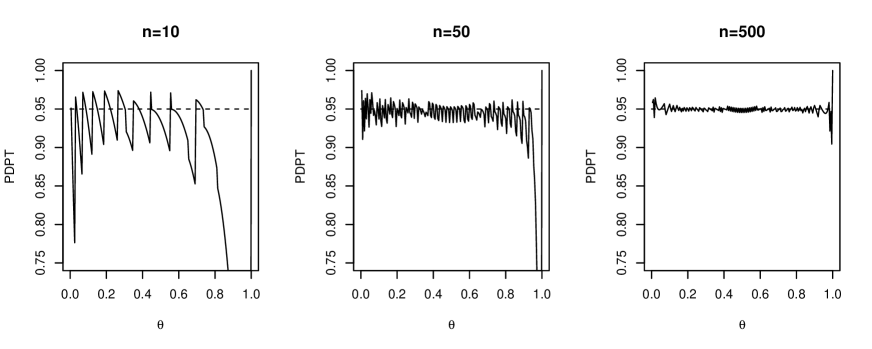
Figure 1: PDPT against the 95% confidence level at $n=10,50,500.$

Figure 1 plots the PDPT of our inferential procedure using the two-sided 95% confidence interval, against confidence level $\int_{{[\hat{\theta}_{l},\hat{\theta}_{u}]}}c(\theta;t)d\theta=0.95$ for $n=10,$ $50$ and $500.$ When $T_{n}=n,$ $C(\theta=1;t=n)=P(G|T_{n}=n)=1$, insuring that $G$ can be accepted with complete confidence (maintaining zero type 1 error). When $T_{n}=t<n,$ $G$ is rejected with complete confidence, and the confidence density $c(\theta;t)$ is the $Beta(t+1,n-t)$ density function to construct the confidence interval for $\theta.$ Figure shows that confidence is a consistent estimator of the objective PDPT for decision process, i.e. confidence converges to the objective probability, namely PDPT as $n$ increases. Our oracle property is achieved in a sacrifice of true PDPT near $\theta=1$ in small sample. Suppose that the true value of $\theta$ is $0.99.$ Because $P_{\theta=0.99}(T_{n}=n)=\theta^{n}=0.90$ if $n=10,$ $P_{\theta=0.99}(T_{n}=n)=0.61$ if $n=50$ and $P_{\theta=0.99}(T_{n}=n)=0.007$ if $n=500,$ PDPT $\leq 0.1$ if $n=10,$ PDPT $\leq 0.39$ if $n=50$ and PDPT $\leq 0.993$ if $n=500$. Thus, when $\theta=0.99,$ our oracle procedure may falsely accept $G$ ($\theta=1$) in small sample. However, $T_{n}$ cannot be $n$ if $n$ is sufficiently large when $\theta<1,$ so that we cannot achieve the false acceptance of $G$ with a sufficiently large data. However, $G$ ($\theta=1$) is still a good approximate scientific theory for $\theta=0.99,$ so that in practice accepting G would be a good practice.

References

1. Bayes, T. (1763). An Essay Towards Solving a Problem in the Doctrine of Chances. By the late Rev. Mr. Bayes, F. R. S. communicated by Mr. Price, in a Letter to John Canton, A. M. F. R. S.. Philosophical transactions of the Royal Society of London, 53, 370-418.

2. Bernardo, J. M. (1979). Reference Posterior Distributions for Bayesian Inference. Journal of the Royal Statistical Society: Series B (Statistical Methodology), 41, 113-128.

3. Broad, C. D. (1918). On the Relation Between Induction and Probability (Part I.). Mind, 27, 389-404.

4. De Finetti, B. (1972). Probability, Induction and Statistics. (London: J. Wiley.)

5. Empiricus, S. (1933). Outlines of Pyrrhonism. (Translated by R. G. Bury. London: W. Heinemann)

6. Etz, A. & Wagenmakers, E. J. (2017). J. B. S. Haldane’s Contribution to the Bayes Factor Hypothesis Test. Statistical Science, 32, 313-329.

7. Fan, J. & Li, R. (2001). Variable Selection via Nonconcave Penalized Likelihood and Its Oracle Properties. Journal of the American statistical Association, 96, 1348-1360.

8. Fisher, R. A. (1921). On the probable error’ of a coefficient of correlation deduced from a small sample. Metron, 1, 1-32.

9. Fisher, R. A. (1930). Inverse Probability. Mathematical Proceedings of the Cambridge Philosophical Society, 26, 528-535.

10. Fisher, R. A. (1935). The Design of Experiments. (Edinburgh: Oliver & Boyd)

11. Fisher, R. A. (1958). The Nature of Probability. Centennial Review of Arts & Science, 2, 261-274.

12. Frank, P. G. (1954). The variety of reasons for the acceptance of scientific theories. The Scientific Monthly, 79, 139-145.

13. Hájek, A. (2007). The Reference Class Problem Is Your Problem Too. Synthese, 156, 563-585.

14. Hartmann, S. & Sprenger, J. (2010). Bayesian Epistemology. (In D. Pritchard & S. Bernecker (Eds.), The Routledge Companion to Epistemology. London: Routledge)

15. Hume, D. (1748). An Enquiry Concerning Human Understanding, P. Millican (Ed.), Oxford: Oxford University Press.

16. Jaynes, E. T. (2003). Probability Theory: The Logic of Science, G. L. Bretthorst (Ed.). (Cambridge: Cambridge University Press)

17. Jeffreys, H. (1939). Theory of Probability. (New York: Oxford University Press)

18. Kant, I. (1781). Critique of Pure Reason. (Translated by W. S. Pluhar. Indianapolis: Hackett)

19. Kaplan, M. (1996). Decision Theory as Philosophy. (Cambridge: Cambridge University Press)

20. Kolmogorov, A. N. (1933). Foundations of Probability. (Translated by N. Morrison. New Yourk: Chelsea Publishing Company)

21. Kuhn, T. S. (2012). The Structure of Scientific Revolutions, 4th ed. with I. Hacking (intro). (University of Chicago Press)

22. Laplace, P. S. (1814). A Philosophical Essay on Probabilities. (Translated by F. W. Truscott & F. L. Emory. New York: Dover.)

23. Lee, Y. & Bjørnstad, J. F. (2013). Extended Likelihood Approach to Large-scale Multiple Testing. Journal of the Royal Statistical Society: Series B (Statistical Methodology), 75, 553-575.

24. Lee, Y. & Nelder, J. A. (1996). Hierarchical Generalized Linear Models (with discussion). Journal of the Royal Statistical Society: Series B (Statistical Methodology), 58, 619-678.

25. Lee, Y. & Nelder, J. A. (2009). Likelihood Inference for Models with Unobservables: Another View (with discussion). Statistical Science, 24, 255-279.

26. Lee, Y., Nelder, J. A. & Pawitan, Y. (2017). Generalized Linear Models with Random Effects: Unified Analysis via H-likelihood, 2nd ed. (Boca Raton, Florida : CRC Press)

27. Lee, Y. & Oh, H. 2014. A New Sparse Variable Selection via Random-effect Model. Journal of Multivariate Analysis, 125, 89-99.

28. Lewis, D. (1980). A Subjectivist Guide to Objective Chance. (In W. L. Harper, R. Stalnaker & G. Pearce (Eds.), Ifs. Berkeley: University of California Press)

29. Neyman, J. (1956). Note on an Article by Sir Ronald Fisher. Journal of the Royal Statistical Society: Series B (Statistical Methodology) , 18, 288-294.

30. Ng, C. T., Lee, W. & Lee, Y. (2018). Change-Point Estimators with True Identification Property. Bernoulli, 24, 616-660.

31. Olsson, E. J. (2018). Bayesian Epistemology. in S. O. Hansson and V. F. Hendricks (eds), Introduction to Formal Philosophy, Springer, Cham.

32. Paulos, J. A. (2011). The Mathematics of Changing Your Mind. New York Times, 5 August 2011.

33. Pawitan, Y. (2001). In All Likelihood: Statistical Modelling and Inference Using Likelihood. (Oxford University Press)

34. Pawitan, Y., Lee, H. & Lee, Y. (2021). Epistemic Confidence, the Dutch Book and Relevant Subsets. arXiv preprint arXiv:2104.14712.

35. Pawitan, Y. & Lee, Y. (2017). Wallet game: Probability, likelihood, and extended likelihood. The American Statistician, 71, 120-122.

36. Pawitan, Y. & Lee, Y. (2021). Confidence as Likelihood. Statistical Science, to appear.

37. Popper, K. R. (1959). New Appendices. (In The Logic of Scientific Discovery. New York: Routledge)

38. Popper, K. R. (1972). Objective knowledge. (Oxford: Oxford University Press)

39. Ramsey, F. P. (1926). Truth and Probability. (In R. B. Braithwaite (Ed.), The Foundations of Mathematics and other Logical Essays. London: Routledge & Kegan Paul)

40. Ross, S. A. (1976). Return, risk and arbitrage. (In I. Friend & J. Bicksler (Eds.), Studies in Risk and Return. Cambridge, MA: Ballinger)

41. Russell, B. (1912). The Problems of Philosophy. (New York: Henry Holt & Co.)

42. Savage, L. J. (1954). The Foundations of Statistics. (New York: Jon Wiley and Sons)

43. Schweder, T. & Hjort, N. L. (2016). Confidence, Likelihood, Probability. (Cambridge University Press)

44. Senn, S. (2003). Dicing with Death: Chance, Risk and Health. (Cambridge University Press)

45. Senn, S. (2009). Comment on Harold Jeffreys’s Theory of Probability Revisited. Statistical Science, 24, 185-186.

46. Von Mises, R. (1928). Probability, Statistics and Truth, 2nd English ed. (Translated by H. Geiringer. London: Allen and Unwin)

47. Von Neumann, J. & Morgenstern, O. (1947). Theory of Games and Economic Behavior, 2nd ed. (Princeton University Press)

48. Xie, M. & Singh, K. (2013). Confidence Distribution, the Frequentist Distribution Estimator of a Parameter: A Review. International Statistical Review, 81, 3-39.