Relational State-Space Model
for Stochastic Multi-Object Systems

Abstract

Real-world dynamical systems often consist of multiple stochastic subsystems that interact with each other. Modeling and forecasting the behavior of such dynamics are generally not easy, due to the inherent hardness in understanding the complicated interactions and evolutions of their constituents. This paper introduces the relational state-space model (R-SSM), a sequential hierarchical latent variable model that makes use of graph neural networks (GNNs) to simulate the joint state transitions of multiple correlated objects. By letting GNNs cooperate with SSM, R-SSM provides a flexible way to incorporate relational information into the modeling of multi-object dynamics. We further suggest augmenting the model with normalizing flows instantiated for vertex-indexed random variables and propose two auxiliary contrastive objectives to facilitate the learning. The utility of R-SSM is empirically evaluated on synthetic and real time series datasets.

1 Introduction

Many real-world dynamical systems can be decomposed into smaller interacting subsystems if we take a fine-grained view. For example, the trajectories of coupled particles are co-determined by per-particle physical properties (e.g., mass and velocity) and their physical interactions (e.g., gravity); traffic flow can be viewed as the coevolution of a large number of vehicle dynamics. Models that are able to better capture the complex behavior of such multi-object systems are of wide interest to various communities, e.g., physics, ecology, biology, geoscience, and finance.

State-space models (SSMs) are a wide class of sequential latent variable models (LVMs) that serve as workhorses for the analysis of dynamical systems and sequence data. Although SSMs are traditionally designed under the guidance of domain-specific knowledge or tractability consideration, recently introduced deep SSMs Fraccaro (2018) use neural networks (NNs) to parameterize flexible state transitions and emissions, achieving much higher expressivity. To develop deep SSMs for multi-object systems, graph neural networks (GNNs) emerge to be a promising choice, as they have been shown to be fundamental NN building blocks that can impose relational inductive bias explicitly and model complex interactions effectively Battaglia et al. (2018).

Recent works that advocate GNNs for modeling multi-object dynamics mostly make use of GNNs in an autoregressive (AR) fashion. AR models based on recurrent (G)NNs can be viewed as special instantiations of SSMs in which the state transitions are restricted to being deterministic (Fraccaro, 2018, Section 4.2). Despite their simplicity, it has been pointed out that their modeling capability is bottlenecked by the deterministic state transitions Chung et al. (2015); Fraccaro et al. (2016) and the oversimplified observation distributions Yang et al. (2018).

In this study, we make the following contributions: (i) We propose the relational state-space model (R-SSM), a novel hierarchical deep SSM that simulates the stochastic state transitions of interacting objects with GNNs, extending GNN-based dynamics modeling to challenging stochastic multi-object systems. (ii) We suggest using the graph normalizing flow (GNF) to construct expressive joint state distributions for R-SSM, further enhancing its ability to capture the joint evolutions of correlated stochastic subsystems. (iii) We develop structured posterior approximation to learn R-SSM using variational inference and introduce two auxiliary training objectives to facilitate the learning.

Our experiments on synthetic and real-world time series datasets show that R-SSM achieves competitive test likelihood and good prediction performance in comparison to GNN-based AR models and other sequential LVMs. The remainder of this paper is organized as follows: Section 2 briefly reviews neccesary preliminaries. Section 3 introduces R-SSM formally and presents the methods to learn R-SSM from observations. Related work is summarized in Section 4 and experimental evaluation is presented in Section 5. We conclude the paper in Section 6.

2 Preliminaries

In this work, an attributed directed graph is given by a 4-tuple: $\mathcal{G}=(\mathcal{V},\mathcal{E},\mathbf{V},{\bm{\mathsfit{E}}})$, where $\mathcal{V}=[N]\coloneqq\{1,\dotsc,N\}$ is the set of vertices, $\mathcal{E}\subseteq[N]\times[N]$ is the set of edges, $\mathbf{V}\in\mathbb{R}^{N\times d_{v}}$ is a matrix of static vertex attributes, and ${\bm{\mathsfit{E}}}\in\mathbb{R}^{N\times N\times d_{e}}$ is a sparse tensor storing the static edge attributes. The set of direct predecessors of vertex $i$ is notated as $\mathcal{N}^{-}_{i}=\left\{p\middle|(p,i)\in\mathcal{E}\right\}$. We use the notation $\mathbf{x}_{i}$ to refer to the $i$-th row of matrix $\mathbf{X}$ and write $\mathbf{x}_{ij}$ to indicate the $(i,j)$-th entry of tensor ${\bm{\mathsfit{X}}}$ (if the corresponding matrix or tensor appears in the context). For sequences, we write $\mathbf{x}_{\leq t}=\mathbf{x}_{1:t}\coloneqq(\mathbf{x}_{1},\ldots,\mathbf{x}_{t})$ and switch to $\mathbf{x}_{t}^{(i)}$ for referring to the $i$-th row of matrix $\mathbf{X}_{t}$.

2.1 Graph Neural Networks

GNNs are a class of neural networks developed to process graph-structured data and support relational reasoning. Here we focus on vertex-centric GNNs that iteratively update the vertex representations of a graph $\mathcal{G}$ while being equivariant Maron et al. (2019) under vertex relabeling. Let $\mathbf{H}\in\mathbb{R}^{N\times d}$ be a matrix of vertex representations, in which the $i$-th row $\mathbf{h}_{i}\in\mathbb{R}^{d}$ is the vectorized representation attached to vertex $i$. Conditioning on the static graph structure and attributes given by $\mathcal{G}$, a GNN just takes the vertex representations $\mathbf{H}$ along with some graph-level context $\mathbf{g}\in\mathbb{R}^{d_{g}}$ as input and returns new vertex representations $\mathbf{H}^{\prime}\in\mathbb{R}^{N\times d^{\prime}}$ as output, i.e., $\mathbf{H}^{\prime}=\text{GNN}(\mathcal{G},\mathbf{g},\mathbf{H})$.

When updating the representation of vertex $i$ from $\mathbf{h}_{i}$ to $\mathbf{h}_{i}^{\prime}$, a GNN takes the representations of other nearby vertices into consideration. Popular GNN variants achieve this through a multi-round message passing paradigm, in which the vertices repeatedly send messages to their neighbors, aggregate the messeages they received, and update their own representations accordingly. Formally, the operations performed by a basic block of a message-passing GNN are defined as follows:

$$\forall(j,i)\in\mathcal{E} : \mathcal{M}_{j\to i} =\text{MESSAGE}\left(\mathbf{g},\mathbf{v}_{j},\mathbf{v}_{i},\mathbf{e}_{ji},\mathbf{h}_{j},\mathbf{h}_{i}\right)$$ (1)

$$\forall i\in\mathcal{V} : \mathcal{A}_{i} =\text{AGGREGATE}\left(\left\{\mathcal{M}_{p\to i}\right\}_{p\in\mathcal{N}^{-}_{i}}\right)$$ (2)

$$\forall i\in\mathcal{V} : \mathbf{h}^{\prime}_{i} =\text{COMBINE}\left(\mathbf{g},\mathbf{v}_{i},\mathbf{h}_{i},\mathcal{A}_{i}\right)$$ (3)

Throughout this work, we implement Equations (1) and (2) by adopting a multi-head attention mechanism similar to Vaswani et al. (2017) and Veličković et al. (2018). For Equation (3), we use either a RNN cell or a residual block He et al. (2016), depending on whether the inputs to GNN are RNN states or not. We write such a block as $\mathbf{H}^{\prime}=\text{MHA}(\mathcal{G},\mathbf{g},\mathbf{H})$ and give its detailed implementation in the Appendix. A GNN simply stacks $L$ separately-parameterized MHA blocks and iteratively computes $\mathbf{H}\eqqcolon\mathbf{H}^{(0)},\ldots,\mathbf{H}^{(L)}\eqqcolon\mathbf{H}^{\prime}$, in which $\mathbf{H}^{(l)}=\text{MHA}(\mathcal{G},\mathbf{g},\mathbf{H}^{(l-1)})$ for $l=1,\ldots,L$. We write this construction as $\mathbf{H}^{\prime}=\text{GNN}(\mathcal{G},\mathbf{g},\mathbf{H})$ and treat it as a black box to avoid notational clutter.

2.2 State-Space Models

State-space models are widely applied to analyze dynamical systems whose true states are not directly observable. Formally, an SSM assumes the dynamical system follows a latent state process $\left\{\mathbf{z}_{t}\right\}_{t\geq 1}$, which possibly depends on exogenous inputs $\{\mathbf{u}_{t}\}_{t\geq 1}$. Parameterized by some (unknown) static parameter $\theta$, the latent state process is characterized by an initial density $\mathbf{z}_{1}\sim\pi_{\theta}(\cdot|\mathbf{u}_{1})$ and a transition density $\mathbf{z}_{t+1}\sim f_{\theta}\left(\cdot\middle|\mathbf{z}_{\leq t},\mathbf{u}_{\leq t+1}\right)$. Moreover, at each time step, some noisy measurements of the latent state are observed through an observation density: $\mathbf{x}_{t}\sim g_{\theta}\left(\cdot\middle|\mathbf{z}_{\leq t},\mathbf{u}_{\leq t}\right)$ . The joint density of $\mathbf{x}_{1:T}$ and $\mathbf{z}_{1:T}$ factors as: $p(\mathbf{x}_{1:T},\mathbf{z}_{1:T}|\mathbf{u}_{1:T})=\pi_{\theta}(\mathbf{z}_{1}|\mathbf{u}_{1})\prod_{t=2}^{T}{f_{\theta}(\mathbf{z}_{t}|\mathbf{z}_{<t},\mathbf{u}_{\leq t})}\prod_{t=1}^{T}{g_{\theta}(\mathbf{x}_{t}|\mathbf{z}_{\leq t},\mathbf{u}_{\leq t})}$.

The superior expressiveness of SSMs can be seen from the fact that the marginal predictive distribution $p(\mathbf{x}_{t}|\mathbf{x}_{<t},\mathbf{u}_{\leq t})=\int p(\mathbf{x}_{t},\mathbf{z}_{\leq t}|\mathbf{x}_{<t},\mathbf{u}_{\leq t})\>\mathrm{d}\mathbf{z}_{\leq t}$ can be far more complex than unimodal distributions and their finite mixtures that are common in AR models. Recently developed deep SSMs use RNNs to compress $\mathbf{z}_{\leq t}$ (and $\mathbf{u}_{\leq t}$) into fixed-size vectors to achieve tractability. As shown in next section, R-SSM can be viewed as enabling multiple individual deep SSMs to communicate.

2.3 Normalizing Flows

Normalizing flows Rezende & Mohamed (2015) are invertible transformations that have the capability to transform a simple probability density into a complex one (or vice versa). Given two domains $\mathcal{X}\subseteq\mathbb{R}^{D}$ and $\mathcal{Y}\subseteq\mathbb{R}^{D}$, let $f:\mathcal{X}\to\mathcal{Y}$ be an invertible mapping with inverse $f^{-1}$. Applying $f$ to a random variable $\mathbf{z}\in\mathcal{X}$ with density $p(\mathbf{z})$, by the change of variables rule, the resulting random variable $\mathbf{z}^{\prime}=f(\mathbf{z})\in\mathcal{Y}$ will have a density:

$$p(\mathbf{z}^{\prime})=p(\mathbf{z})\left|\det\frac{\partial f^{-1}}{\partial\mathbf{z}^{\prime}}\right|=p(\mathbf{z})\left|\det\frac{\partial f}{\partial\mathbf{z}}\right|^{-1}$$

A series of invertible mappings with cheap-to-evaluate determinants can be chained together to achieve complex transformations while retaining efficient density calculation. This provides a powerful way to construct expressive distributions.

3 Relational State-Space Model

Suppose there is a dynamical system that consists of multiple interacting objects, and observing this system at a specific time is accomplished by acquiring measurements from every individual object simultaneously. We further assume these objects are homogeneous, i.e., they share the same measurement model, and leave systems whose constituents are nonhomogeneous for future work. To generatively model a time-ordered series of observations collected from this system, the straightforward approach that builds an individual SSM for each object is usually unsatisfactory, as it simply assumes the state of each object evolves independently and ignores the interactions between objects. To break such an independence assumption, our main idea is to let multiple individual SSMs interact through GNNs, which are expected to capture the joint state transitions of correlated objects well.

[width=]img/generative-model

(a) Generative model.

[width=]img/generative-model-collapsed

(b) Collapsed generative model.

[width=]img/proposal

(c) Inference model.

Figure 1: Graphical structures of R-SSM. Diamonds represent deterministic states and circles represent random variables. To be concise, the dependencies on the graph $\mathcal{G}$ and exogenous inputs $\mathbf{U}_{1:T}$ are not shown. (b) is the result of collapsing all deterministic states in (a) and writing $\mathcal{Z}_{t}=(\mathbf{z}_{t}^{g},\mathbf{Z}_{t})$. In (c), solid lines represent the computation shared with the generative model and dashed lines represent additional computation for inference.

3.1 Generative model

Given the observations for a multi-object dynamical system, our model further assumes its interaction structure is known as prior knowledge. The interaction structure is provided as a directed graph, in which each object corresponds to a vertex, and a directed edge indicates that the state of its head is likely to be affected by its tail. In situations where such graph structure is not available, a complete graph can be specified. However, to model dynamical systems comprising a large number of objects, it is often beneficial to explicitly specify sparse graph structures, because they impose stronger relational inductive bias and help save the computational cost.

A relational state-space model assumes a set of correlated dynamical subsystems evolve jointly under the coordination of graph neural networks. Formally, given a graph $\mathcal{G}=(\mathcal{V},\mathcal{E},\mathbf{V},{\bm{\mathsfit{E}}})$, in which an edge $(i,j)\in\mathcal{E}$ indicates that the state of vertex $j$ may be affected by vertex $i$. Let $\mathbf{u}_{t}^{(i)}\in\mathbb{R}^{d_{u}}$ and $\mathbf{x}_{t}^{(i)}\in\mathbb{R}^{d_{x}}$ be the input and observation for vertex $i$ at time step $t$, respectively. For $T$ steps, we introduce a set of unobserved random variables $\{\mathbf{z}_{1:T}^{(i)}\}_{i=1}^{N}$, in which $\mathbf{z}_{t}^{(i)}\in\mathbb{R}^{d_{z}}$ represents the latent state of vertex $i$ at time step $t$. Furthermore, we introduce a global latent variable $\mathbf{z}_{t}^{g}\in\mathbb{R}^{d_{g}}$ for each time step to represent the global state shared by all vertices. Conditioning on the graph and exogenous inputs, an R-SSM factorizes the joint density of observations and latent states as follows:

$$p_{\theta}\left(\big{\{}\mathbf{x}_{1:T}^{(i)}\big{\}}_{i=1}^{N},\big{\{}\mathbf{z}_{1:T}^{(i)}\big{\}}_{i=1}^{N},\mathbf{z}_{1:T}^{g}\middle|\mathcal{G},\big{\{}\mathbf{u}_{1:T}^{(i)}\big{\}}_{i=1}^{N}\right)=\\ \prod_{t=1}^{T}{f_{\theta}\left(\big{\{}\mathbf{z}_{t}^{(i)}\big{\}}_{i=1}^{N},\mathbf{z}_{t}^{g}\middle|\big{\{}\mathbf{z}_{<t}^{(i)}\big{\}}_{i=1}^{N},\mathbf{z}_{<t}^{g},\mathcal{G},\big{\{}\mathbf{u}_{\leq t}^{(i)}\big{\}}_{i=1}^{N}\right)}\\ \prod_{t=1}^{T}{\prod_{i=1}^{N}{g_{\theta}\left(\mathbf{x}_{t}^{(i)}\middle|\mathbf{z}_{t}^{(i)},\mathbf{z}_{\leq t}^{g},\big{\{}\mathbf{z}_{<t}^{(i)}\big{\}}_{i=1}^{N},\mathcal{G},\big{\{}\mathbf{u}_{\leq t}^{(i)}\big{\}}_{i=1}^{N}\right)}}$$ (4)

For notational simplicity, we switch to the matrix notation $\mathbf{Z}_{t}=\big{[}\mathbf{z}_{t}^{(1)},\mathbf{z}_{t}^{(2)},\ldots,\mathbf{z}_{t}^{(N)}\big{]}^{\top}$ from now on. The joint transition density $f_{\theta}$ is further factorized as a product of global transition density $f_{\theta}^{g}$ and local transition density $f_{\theta}^{\star}$, i.e., $f_{\theta}\left(\mathbf{Z}_{t},\mathbf{z}_{t}^{g}\middle|\ldots\right)=f_{\theta}^{g}\left(\mathbf{z}_{t}^{g}\middle|\ldots\right)f_{\theta}^{\star}\left(\mathbf{Z}_{t}\middle|\mathbf{z}_{t}^{g},\ldots\right)$ . To instantiate these conditional distributions, a GNN accompanied by RNN cells is adopted to recurrently compress the past dependencies at each time step into fixed-size context vectors. Specifically, the observations are assumed to be generated from following process:

$$\tilde{\mathbf{h}}_{t}^{(i)}=\text{RNN}_{\theta}^{v}\big{(}\mathbf{h}_{t-1}^{(i)},\big{[}\mathbf{z}_{t-1}^{(i)},\mathbf{u}_{t}^{(i)}\big{]}\big{)},\quad \tilde{\mathbf{h}}_{t}^{g}=\text{READOUT}_{\theta}\big{(}\mathcal{G},\tilde{\mathbf{H}}_{t}\big{)}$$

$$\mathbf{h}_{t}^{g}=\text{RNN}_{\theta}^{g}\big{(}\mathbf{h}_{t-1}^{g},\big{[}\mathbf{z}_{t-1}^{g},\tilde{\mathbf{h}}_{t}^{g}\big{]}\big{)},\quad \mathbf{z}_{t}^{g}\sim f_{\theta}^{g}\big{(}\cdot\big{|}\mathbf{h}_{t}^{g}\big{)}$$

$$\mathbf{H}_{t}=\text{GNN}_{\theta}\big{(}\mathcal{G},\mathbf{z}_{t}^{g},\tilde{\mathbf{H}}_{t}\big{)},\quad \mathbf{Z}_{t}\sim f_{\theta}^{\star}\big{(}\cdot\big{|}\mathbf{H}_{t}\big{)}$$

$$\mathbf{x}_{t}^{(i)}\sim g_{\theta}\big{(}\cdot\big{|}\mathbf{z}_{t}^{(i)},\mathbf{h}_{t}^{(i)},\mathbf{z}_{t}^{g},\mathbf{h}_{t}^{g}\big{)}$$

for $i=1,\ldots,N$ and $t=1,\ldots,T$, where $\mathbf{h}_{0}^{(i)}=\mathbf{h}_{0}^{\ast}$ and $\mathbf{z}_{0}^{(i)}=\mathbf{z}_{0}^{\ast}$. Here $\mathbf{h}_{0}^{g}$, $\mathbf{z}_{0}^{g}$, $\mathbf{h}_{0}^{\ast}$ and $\mathbf{z}_{0}^{\ast}$ are learnable initial states. The READOUT function aggregates the context vectors of all vertices into a global context vector in a permutation-invariant manner. The global transition density $f_{\theta}^{g}$ is specified to be a diagonal Gaussian distribution whose mean and variance are parameterized by the output of a multilayer perceptron (MLP), and the local transition density $f_{\theta}^{\star}$ will be discussed later. The local observation distribution $g_{\theta}$ can be freely selected in line with the data, and in our experiments it is either a Gaussian distribution or a mixture of logistic distributions parameterized by MLPs.

The graphical structure of two consecutive steps of the generating process is illustrated in Figure 1(a). An intuitive way to think about this generative model is to note that the $N+1$ latent state processes interact through the GNN, which enables the new state of a vertex to depend on not only its own state trajectory but also the state trajectories of other vertices and the entire graph.

3.2 Learning and inference

As illustrated in Figure 1(b), writing $\mathcal{Z}_{t}=(\mathbf{z}_{t}^{g},\mathbf{Z}_{t})$ and suppressing the dependencies on the graph $\mathcal{G}$ and exogenous inputs $\mathbf{U}_{1:T}$, an R-SSM can be interpreted as an ordinary SSM in which the entire graph evolves as a whole, i.e., the joint density of latent states and observations factors as: $p(\mathbf{X}_{1:T},\mathcal{Z}_{1:T})=\prod_{t=1}^{T}{p_{\theta}(\mathcal{Z}_{t}|\mathcal{Z}_{<t})p_{\theta}(\mathbf{X}_{t}|\mathcal{Z}_{t})}$. Given observations $\mathbf{X}_{1:T}$, we are interested in learning unknown parameters $\theta$ and inferring unobserved states $\mathcal{Z}_{1:T}$. For the learning task we wish to maximize the marginal likelihood $p_{\theta}(\mathbf{X}_{1:T})=\int p_{\theta}(\mathbf{X}_{1:T},\mathcal{Z}_{1:T})\>\mathrm{d}\mathcal{Z}_{1:T}$, but in our case the integral is intractable. We adopt a recently developed variational inference (VI) approach called variational sequential Monte Carlo (VSMC) Maddison et al. (2017); Naesseth et al. (2018); Le et al. (2018), which maximizes a variational lower bound on the log marginal likelihood instead and learns the proposal distributions for the inference task simultaneously.

Given a sequence of proposal distributions $\{q_{\phi}\left(\mathcal{Z}_{t}\middle|\mathcal{Z}_{<t},\mathbf{X}_{\leq t}\right)\}_{t=1}^{T}$ parameterized by $\phi$, running the sequential Monte Carlo (SMC) algorithm with $K$ particles yields an unbiased marginal likelihood estimator $\hat{p}_{\theta,\phi,K}(\mathbf{X}_{1:T})=\prod_{t=1}^{T}{\big{[}\nicefrac{{1}}{{K}}\sum_{k=1}^{K}{w_{t}^{k}}\big{]}}$, where $w_{t}^{k}$ is the unnormalized importance weight of particle $k$ at time $t$. The variational lower bound is obtained by applying the Jensen’s inequality:

$$\mathcal{L}_{K}^{\text{SMC}}(\theta,\phi)\coloneqq\mathbb{E}\left[\log\hat{p}_{\theta,\phi,K}(\mathbf{X}_{1:T})\right]\leq\log\mathbb{E}\left[\hat{p}_{\theta,\phi,K}(\mathbf{X}_{1:T})\right]=\log p_{\theta}(\mathbf{X}_{1:T})$$ (5)

Assuming the proposal distributions are reparameterizable Kingma & Welling (2014), we use the biased gradient estimator $\nabla\mathcal{L}_{K}^{\text{SMC}}(\theta,\phi)\approx\mathbb{E}[\nabla\log\hat{p}_{\theta,\phi,K}(\mathbf{X}_{1:T})]$ to maximize $\mathcal{L}_{K}^{\text{SMC}}$.

Proposal design.

We make the proposal for $\mathcal{Z}_{t}$ depend on the information up to time $t$ and share some parameters with the generative model. We also choose to factorize $q_{\phi}\left(\mathcal{Z}_{t}\middle|\ldots\right)=r_{\phi}^{g}\left(\mathbf{z}^{g}_{t}\middle|\ldots\right)r_{\phi}^{\star}\left(\mathbf{Z}_{t}\middle|\mathbf{z}^{g}_{t},\ldots\right)$ . The proposal distributions for all time steps are structured as follows:

$$\tilde{\mathbf{b}}_{t}^{(i)}=\text{RNN}_{\phi}\big{(}\mathbf{b}_{t-1}^{(i)},\big{[}\mathbf{x}_{t}^{(i)},\mathbf{u}_{t}^{(i)}\big{]}\big{)},\quad \tilde{\mathbf{b}}_{t}^{g}=\text{READOUT}_{\phi,1}\big{(}\mathcal{G},\tilde{\mathbf{B}}_{t}\big{)}$$

$$\mathbf{B}_{t}=\text{GNN}_{\phi}\big{(}\mathcal{G},\tilde{\mathbf{b}}_{t}^{g},\tilde{\mathbf{B}}_{t}\big{)},\quad \mathbf{b}_{t}^{g}=\text{READOUT}_{\phi,2}\big{(}\mathcal{G},\mathbf{B}_{t}\big{)}$$

$$\mathbf{z}_{t}^{g}\sim r_{\phi}^{g}\big{(}\cdot\big{|}\mathbf{h}_{t}^{g},\mathbf{b}_{t}^{g}\big{)},\quad \mathbf{Z}_{t}\sim r_{\phi}^{\star}\big{(}\cdot\big{|}\mathbf{H}_{t},\mathbf{B}_{t}\big{)}$$

for $i=1,\ldots,N$ and $t=1,\ldots,T$, where $\mathbf{h}_{t}^{g}$ and $\mathbf{H}_{1:T}$ are computed using the relevant parts of the generative model. $r_{\phi}^{g}$ is specified to be a diagonal Gaussian parameterized by an MLP, and $r_{\phi}^{\star}$ will be discussed soon. Here $\mathbf{B}_{t}$ can be interpreted as a belief state Gregor et al. (2019), which summarizes past observations $\mathbf{X}_{\leq t}$ (and inputs $\mathbf{U}_{\leq t}$) deterministically. The graphical structure of this proposal design is shown in Figure 1(c), and the detailed VSMC implementation using this proposal is given in Appendix A.4.

3.3 Graph Normalizing Flow

The local transition density $f_{\theta}^{\star}\left(\mathbf{Z}_{t}\big{|}\ldots\right)$ and the local proposal density $r_{\phi}^{\star}\left(\mathbf{Z}_{t}\middle|\ldots\right)$ may be parameterized in several ways. One simple and efficient starting point is (block-)diagonal Gaussian distribution: $f_{\theta}^{\star}\left(\mathbf{Z}_{t}\big{|}\ldots\right)=\prod_{i=1}^{N}\mathcal{N}(\mathbf{z}_{t}^{(i)}|\ldots)$, which assumes that the object states are conditionally independent, i.e., the joint state distribution is completely factorized over objects. We believe that such an independence assumption is an oversimplification for situations where the joint state evolution is multimodal and highly correlated. One possible way to introduce inter-object dependencies is modeling joint state distributions as Markov random fields (MRFs) Naesseth et al. (2019), but this will significantly complicate the learning.

Here we introduce the Graph Normalizing Flow (GNF) , which adapts Glow Kingma & Dhariwal (2018) to graph settings and enables us to build expressive joint distributions for correlated random variables indexed by graph nodes. As described earlier, the key ingredient for a flow is a series invertible mappings that are iteratively applied to the samples of a base distribution. Now we are interested in the case where the samples are vertex states $\mathbf{Z}_{t}$, and thus the invertible mappings should be further constrained to be equivariant under vertex relabeling. This rules out popular autoregressive flows, e.g., IAF Kingma et al. (2016) and MAF Papamakarios et al. (2017).

Our GNF is built upon the coupling layer introduced in Dinh et al. (2017), which provides a flexible framework to construct efficient invertible mappings. A GNF coupling layer splits the input $\mathbf{Z}\in\mathbb{R}^{N\times D}$ into two parts, $\mathbf{Z}_{a}\in\mathbb{R}^{N\times d}$ and $\mathbf{Z}_{b}\in\mathbb{R}^{N\times(D-d)}$. The output $\mathbf{Z}^{\prime}\in\mathbb{R}^{N\times D}$ is formed as:

$$\mathbf{Z}^{\prime}_{a}=\mathbf{Z}_{a}\;,\quad\mathbf{Z}^{\prime}_{b}=\mathbf{Z}_{b}\odot\exp\big{(}s(\mathbf{Z}_{a})\big{)}+t(\mathbf{Z}_{a})\;,\quad\mathbf{Z}^{\prime}=[\mathbf{Z}^{\prime}_{a},\mathbf{Z}^{\prime}_{b}]\;,$$

where $\odot$ denotes the element-wise product, and the functions $s(\cdot)$ and $t(\cdot)$ are specified to be GNNs to enforce the equivariance property. A GNF combines a coupling layer with a trainable element-wise affine layer and an invertible $1\times 1$ convolution layer Hoogeboom et al. (2019), organizing them as: $\text{Input}\rightarrow\text{Affine}\rightarrow\text{Coupling}\rightarrow\text{Conv}_{1\times 1}\rightarrow\text{Output}$. A visual illustration of this architecture is provided in Appendix A.5.

In order to obtain more expressive prior and variational posterior approximation, the local transition density and local proposal density can be constructed by stacking multiple GNFs on top of diagonal Gaussian distributions parameterized by MLPs. With the message passing inside the coupling layers, GNFs can transform independent noise into correlated noise and thus increase model expressivity. The $1\times 1$ convolution layers free us from manually permuting the dimensions, and the element-wise affine layers enable us to tune their initial weights to stablize training.

3.4 Auxiliary contrastive prediction tasks

In our initial experiments, we found that learning R-SSM suffered from the posterior collpase phenomenon, which is a well known problem in the training of variational autoencoders (VAEs). It means that the variational posterior approximation $q_{\phi}(\mathcal{Z}_{t}|\mathcal{Z}_{<t},\mathbf{X}_{\leq t})$ degenerate into the prior $f_{\theta}(\mathcal{Z}_{t}|\mathcal{Z}_{<t})$ in the early stage of optimization, making the training dynamics get stuck in undesirable local optima. Besides, we also encountered a more subtle problem inherent in likelihood-based training of deep sequential models. That is, for relatively smooth observations, the learned model tended to only capture short-term local correlations but not the interaction effects and long-term transition dynamics.

Motivated by recent advances in unsupervised representation learning based on mutual information maximization, in particular the Contrastive Predictive Coding (CPC) approach Oord et al. (2018), we alleviate these problems by forcing the latent states to perform two auxiliary contrastive prediction tasks. At each time step $t$, the future observations of each vertex $i$ are summarized into a vector using a backward RNN: $\mathbf{c}_{t}^{(i)}=\text{RNN}_{\psi}(\mathbf{x}_{>t}^{(i)})$. Then we define two auxiliary CPC objectives:

$$\mathcal{L}_{1}^{\text{aux}}=\mathbb{E}\left[\sum_{t=1}^{T-1}\sum_{i=1}^{N}\log\frac{\lambda_{\psi,1}(\hat{\mathbf{z}}_{t}^{(i)},\mathbf{c}_{t}^{(i)})}{\sum_{\mathbf{c}\in\Omega_{t,i}}{\lambda_{\psi,1}(\hat{\mathbf{z}}_{t}^{(i)},\mathbf{c})}}\right],\;\mathcal{L}_{2}^{\text{aux}}=\mathbb{E}\left[\sum_{t=1}^{T-1}\sum_{i=1}^{N}\log\frac{\lambda_{\psi,2}(\hat{\mathbf{h}}_{t}^{(i)},\mathbf{c}_{t}^{(i)})}{\sum_{\mathbf{c}\in\Omega_{t,i}}{\lambda_{\psi,2}(\hat{\mathbf{h}}_{t}^{(i)},\mathbf{c})}}\right]$$

where $\hat{\mathbf{z}}_{t}^{(i)}=[\mathbf{z}_{t}^{g},\mathbf{z}_{t}^{(i)}]$, $\hat{\mathbf{h}}_{t}^{(i)}=\text{MLP}_{\psi}(\sum_{j\neq i\,\wedge\,j\in\mathcal{N}_{i}^{-}}{\mathbf{h}_{t}^{(j)}})$, and $\Omega_{t,i}$ is a set that contains $\mathbf{c}_{t}^{(i)}$ and some negative samples. The expectation is over negative samples and the latent states sampled from the filtering distributions. The positive score functions $\lambda_{\psi,1}$ and $\lambda_{\psi,2}$ are specified to be simple log-bilinear models.

Intuitively, $\mathcal{L}_{1}^{\text{aux}}$ encourages the latent states to encode useful information that helps distinguish the future summaries from negative samples. $\mathcal{L}_{2}^{\text{aux}}$ encourages the deterministic states to reflect the interaction effects, as it contrastingly predicts the future summary of vertex $i$ based on the states of $i$’s neighbors only. The negative samples are selected from the future summaries of other vertices within the minibatch. The final objective to maximize is $\mathcal{L}=\mathcal{L}_{K}^{\text{SMC}}+\beta_{1}\mathcal{L}_{1}^{\text{aux}}+\beta_{2}\mathcal{L}_{2}^{\text{aux}}$, in which $\beta_{1}\geq 0$ and $\beta_{2}\geq 0$ are tunable hyperparameters. The procedure to estimate this objective is described in Appendix A.4.

4 Related Work

GNN-based dynamics modeling.

GNNs Scarselli et al. (2009); Duvenaud et al. (2015); Li et al. (2016); Defferrard et al. (2016); Gilmer et al. (2017); Hamilton et al. (2017); Veličković et al. (2018); Xu et al. (2019); Maron et al. (2019) provide a promising framework to learn on graph-structured data and impose relational inductive bias in learning models. We refer the reader to Battaglia et al. (2018) for a recent review. GNNs (or neural message passing modules) are the core components of recently developed neural physics simulators Battaglia et al. (2016); Watters et al. (2017); Chang et al. (2017); Janner et al. (2019); Sanchez-Gonzalez et al. (2018); Mrowca et al. (2018); Li et al. (2019) and spatiotemporal or multi-agent dynamics models Alahi et al. (2016); Hoshen (2017); Li et al. (2018); Zhang et al. (2018); Tacchetti et al. (2019); chen-aaai2020. In these works, GNNs usually act autoregressively or be integrated into the sequence-to-sequence (seq2seq) framework Sutskever et al. (2014). Besides, recently they have been combined with generative adversarial networks Goodfellow et al. (2014) and normalizing flows for multi-agent forecasting Gupta et al. (2018); Kosaraju et al. (2019); Rhinehart et al. (2019). R-SSM differs from all these works by introducing structured latent variables to represent the uncertainty on state transition and estimation.

GNNs in sequential LVMs.

A few recent works have combined GNNs with a sequential latent variable model, including R-NEM van Steenkiste et al. (2018), NRI Kipf et al. (2018), SQAIR Kosiorek et al. (2018), VGRNN Hajiramezanali et al. (2019), MFP Tang & Salakhutdinov (2019), and Graph VRNN Sun et al. (2019); Yeh et al. (2019). The latent variables in R-NEM and NRI are discrete and represent membership relations and types of edges, respectively. In contrast, the latent variables in our model are continuous and represent the states of objects. SQAIR is also a deep SSM for multi-object dynamics, but the GNN is only used in its inference network. VGRNN is focused on modeling the topological evolution of dynamical graphs. MFP employs a conditional VAE architecture, in which the per-agent discrete latent variables are shared by all time steps. The work most relevant to ours is Graph VRNN, in which the hidden states of per-agent VRNNs interact through GNNs. Our work mainly differs from it by introducing a global latent state process to make the model hierarchical and exploring the use of normalizing flows as well as the auxiliary contrastive objectives. More subtle differences are discussed in Section 5.2.

Deep LVMs for sequential data.

There has been growing interest in developing latent variable models for sequential data with neural networks as their building blocks, among which the works most relevant to ours are stochastic RNNs and deep SSMs. Many works have proposed incorporating stochastic latent variables into vanilla RNNs to equip them with the ability to express more complex data distributions Bayer & Osendorfer (2014); Chung et al. (2015); Fraccaro et al. (2016); Goyal et al. (2017); Ke et al. (2019) or, from another perspective, developing deep SSMs by parameterizing flexible transition and emission distributions using neural networks Krishnan et al. (2017); Fraccaro et al. (2017); Buesing et al. (2018); Zheng et al. (2017); Hafner et al. (2019). Approximate inference and parameter estimation methods for nonlinear SSMs have been extensively studied in the literature Doucet & Johansen (2009); Andrieu et al. (2010); Kantas et al. (2015); Gu et al. (2015); Karl et al. (2016); Marino et al. (2018); Gregor et al. (2019); Hirt & Dellaportas (2019). We choose VSMC Maddison et al. (2017); Naesseth et al. (2018); Le et al. (2018) as it combines the powers of VI and SMC. The posterior collapse problem is commonly addressed by KL annealing, which does not work with VSMC. The idea of using auxiliary costs to train deep SSMs has been explored in Z-forcing Goyal et al. (2017); Ke et al. (2019), which predicts the future summaries directly rather than contrastingly. As a result, the backward RNN in Z-forcing may degenerate easily.

5 Experiments

We implement R-SSM using the TensorFlow Probability library Dillon et al. (2017). The experiments are organized as follows: In Section 5.1, we sample a toy dataset from a simple stochastic multi-object model and validate that R-SSM can fit it well while AR models and non-relational models may struggle. In Section 5.2, R-SSM is compared with state-of-the-art sequential LVMs for multi-agent modeling on a basketball gameplay dataset, and the effectiveness of GNF is tested through ablation studies. Finally, in Section 5.3, the prediction performance of R-SSM is compared with strong GNN-based seq2seq baselines on a road traffic dataset. Due to the space constraint, the detailed model architecture and hyperparameter settings for each dataset are given in the Appendix. Below, all values reported with error bars are averaged over 3 or 5 runs.

5.1 Synthetic toy dataset

First we construct a simple toy dataset to illustrate the capability of R-SSM. Each example in this dataset is generated by the following procedure:

$$\mathcal{G}\sim\text{SBM}(N,K,p_{0},p_{1}),\quad\mathbf{v}_{i}\sim\text{Normal}(\mathbf{0},\mathbf{I}),\quad z_{0}^{(i)}\sim\text{Normal}(0,1)$$

$$\tilde{z}_{t}^{(i)}=\bm{\eta}^{\top}\mathbf{v}_{i}+\alpha_{1}{\textstyle\sum}_{j\in\mathcal{N}_{i}}{z_{t-1}^{(j)}}/|\mathcal{N}_{i}|+\alpha_{2}z_{t-1}^{(i)}$$ (6)

$$z_{t}^{(i)}\sim\text{Normal}\big{(}\cos(\tilde{z}_{t}^{(i)}),\sigma_{z}^{2}\big{)},\quad x_{t}^{(i)}\sim\text{Normal}\big{(}\tanh(\varepsilon z_{t}^{(i)}),\sigma_{x}^{2}\big{)}$$

for $i=1,\ldots,N$ and $t=1,\ldots,T$. Here SBM is short for the symmetric stochastic block model, in which each vertex $i$ belongs to exact one of the $K$ communities, and two vertices $i$ and $j$ are connected with probability $p_{0}$ if they are in the same community, $p_{1}$ otherwise. A vertex-specific covariate vector $\mathbf{v}_{i}\in\mathbb{R}^{d_{v}}$ is attached to each vertex $i$, and by Equation (6), the state of each vertex $i$ can be affected by its neighbors $\mathcal{N}_{i}$. Choosing the parameters $d_{v}=4$, $N=36$, $K=3$, $p_{0}=1/3$, $p_{1}=1/18$, $T=80$, $\alpha_{1}=5.0$, $\alpha_{2}=-1.5$, $\bm{\eta}=[-1.5,0.4,2.0,-0.9]^{\top}$, $\sigma_{x}=\sigma_{z}=0.05$, and $\varepsilon=2.5$, we generate 10K examples for training, validation, and test, respectively. A typical example is visualized in the Appendix.

Despite the simple generating process, the resulting dataset is highly challenging for common models to fit. To show this, we compare R-SSM with several baselines, including (a) VAR: Fitting a first-order vector autoregression model for each example; (b) VRNN: A variational RNN Chung et al. (2015) shared by all examples; (c) GNN-AR: A variant of the recurrent decoder of NRI Kipf et al. (2018), which is exactly a GNN-based AR model when given the ground-truth graph. VAR and VRNN are given access to the observations $\{x_{1:T}^{(i)}\}_{i=1}^{N}$ only, while GNN-AR and R-SSM are additionally given access to the graph structure $(\mathcal{V},\mathcal{E})$ (but not the vertex covariates). GNF is not used in R-SSM because the true joint transition distribution is factorized over vertices.

Table 1: Test log-likelihood and prediction performance comparisons on the synthetic toy dataset.

Model	LL	MSE	CP
VAR	-366	0.679 $\pm$.000	0.750 $\pm$.000
VRNN	$\geq$-2641	0.501 $\pm$.003	0.931 $\pm$.002
GNN-AR	-94	0.286 $\pm$.002	0.806 $\pm$.004
R-SSM	$\geq$2583	0.029 $\pm$.001	0.883 $\pm$.002
$+\mathcal{L}_{2}^{\text{aux}}$	$\geq$2647	0.024 $\pm$.001	0.897 $\pm$.001

For each model, we calculate three metrics: (1) LL: Average log-likelihood (or its lower bound) of test examples; (2) MSE: Average mean squared one-step prediction error given the first 75 time steps of each test example; (3) CP: Average coverage probability of a 90% one-step prediction interval. For non-analytic models, point predictions and prediction intervals are computed using 1000 Monte Carlo samples. The results are reported in Table 1.

The generating process involves latent factors and nonlinearities, so VAR performs poorly as expected. VRNN largely underfits the data and struggles to generalize, which may be caused by the different topologies under the examples. In contrast, GNN-AR and R-SSM generalize well as expected, while R-SSM achieves much higher test log-likelihood and produces good one-step probabilistic predictions. This toy case illustrates the generalization ability of GNNs and suggests the importance of latent variables for capturing the uncertainty in stochastic multi-object systems. We also observed that without $\mathcal{L}_{1}^{\text{aux}}$ the training dynamics easily get stuck in posterior collapse at the very early stage, and adding $\mathcal{L}_{2}^{\text{aux}}$ help improve the test likelihood.

Table 2: Test log-likelihood and rollout quality comparisons on the basketball gameplay dataset (offensive players only).

Model	$\mathcal{L}_{1000}^{\text{SMC}}$	ELBO	Speed	Distance	OOB
VRNN	—	2360	0.89	43.78	33.78
MI-VRNN	—	2362	0.79	38.92	15.52
R-SSM	2459.8 $\pm$.3	2372.3 $\pm$.8	0.83 $\pm$.01	40.75 $\pm$.15	1.84 $\pm$.16
$+\mathcal{L}_{2}^{\text{aux}}$	2463.3 $\pm$.4	2380.2 $\pm$.6	0.82 $\pm$.01	40.36 $\pm$.23	2.17 $\pm$.09
$+$GNF (4)	2483.2 $\pm$.3	2381.6 $\pm$.4	0.80 $\pm$.00	39.37 $\pm$.35	2.06 $\pm$.15
$+$GNF (8)	2501.6 $\pm$.2	2382.1 $\pm$.4	0.79 $\pm$.00	39.14 $\pm$.29	2.12 $\pm$.10
Ground Truth	—	—	0.77	37.78	2.21

5.2 Basketball gameplay

In basketball gameplay, the trajectories of players and the ball are highly correlated and demonstrate rich, dynamic interations. Here we compare R-SSM with a state-of-the-art hierarchical sequential LVM for multi-agent trajectories Zhan et al. (2019), in which the per-agent VRNNs are coordinated by a global "macro intent" model. We note it as MI-VRNN. The dataset includes 107,146 training examples and 13,845 test examples, each of which contains the 2D trajectories of ten players and the ball recorded at 6Hz for 50 time steps. Following their settings, we use the trajectories of offensive team only and preprocess the data in exactly the same way to make the results directly comparable. The complete graph of players is used as the input to R-SSM.

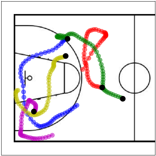
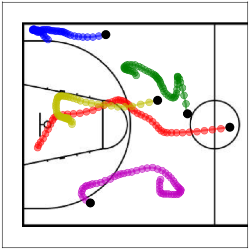
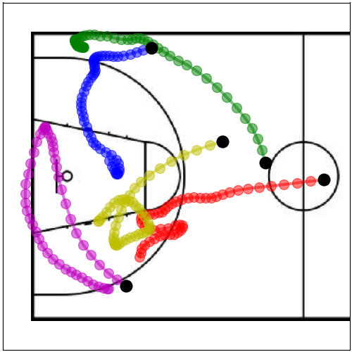
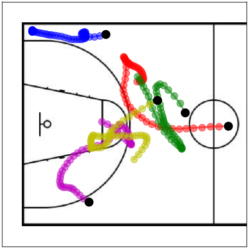
Several ablation studies are performed to verify the utility of the proposed ideas. In Table 4, we report test likelihood bounds and the rollout quality evaluated with three heuristic statistics: average speed (feet/step), average distance traveled (feet), and the percentage of out-of-bound (OOB) time steps. The VRNN baseline developed by Zhan et al. (2019) is also included for comparison. Note that the VSMC bound $\mathcal{L}_{1000}^{\text{SMC}}$ is a tighter log-likelihood approximation than the ELBO (which is equivalent to $\mathcal{L}_{1}^{\text{SMC}}$). The rollout statistics of R-SSMs are calculated from 150K 50-step rollouts with 10 burn-in steps. Several selected rollouts are visualized in the Appendix.

As illustrated in Table 2, all R-SSMs outperform the baselines in terms of average test log-likelihood. Again, we observed that adding $\mathcal{L}_{1}^{\text{aux}}$ is necessary for training R-SSM successfully on this dataset. Training with the proposed auxiliary loss $\mathcal{L}_{2}^{\text{aux}}$ and adding GNFs do improve the results. R-SSM with 8 GNFs (4 in prior, 4 in proposal) achieves higher likelihood than R-SSM with 4 GNFs, indicating that increasing the expressivity of joint state distributions helps fit the data better. As for the rollout quality, the OOB rate of the rollouts sampled from our model matches the ground-truth significantly better, while the other two statistics are comparable to the MI-VRNN baseline.

In Table 4, we also provide preliminary results for the setting that additionally includes the trajectory of the ball. This enables us to compare with the results reported by Yeh et al. (2019) for Graph VRNN (GVRNN). The complete graph of ball and players served as input to R-SSM is annotated with two node types (player or ball) and three edge types (player-to-ball, ball-to-player or player-to-player). R-SSM achieves competitive test likelihood, and adding GNFs helps improve the performance. We point out that several noticeable design choices of GVRNN may help it outperform R-SSM: (i) GVRNN uses a GNN-based observation model, while R-SSM uses a simple factorized observation model. (ii) GVRNN encodes $\mathbf{X}_{1:t-1}$ into $\mathbf{H}_{t}$ and thus enables the prior of $\mathbf{Z}_{t}$ to depend on past observations, which is not the case in R-SSM. (iii) GVRNN uses several implementation tricks, e.g., predicting the changes in observations only ($\mathbf{X}_{t}=\mathbf{X}_{t-1}+{\Delta\mathbf{X}}_{t}$) and passing raw observations as additional input to GNNs. We would like to investigate the effect of these interesting differences in future work.

Table 3: Test log-likelihood comparison on the basketball gameplay dataset (offensive players plus the ball).

Model	LL	$\mathcal{L}_{1000}^{\text{SMC}}$
Yeh et al. (2019)
GRNN	2264	—
VRNN	$>$2750	—
GVRNN	$>$2832	—
R-SSM$+\mathcal{L}_{2}^{\text{aux}}$	$>$2761 $\pm$1	2805 $\pm$0
$+$GNF (8)	$>$2783 $\pm$1	2826 $\pm$0

Table 4: Forecast MAE comparison on the METR-LA dataset. $h$ is the number of steps predicted into the future. The $\mathbf{X}_{t-h}$ baseline outputs $\mathbf{X}_{t-h}$ to predict $\mathbf{X}_{t}$.

Model	$h=3$	$h=6$	$h=12$
$\mathbf{X}_{t-h}$	3.97	4.99	6.65
DCRNN	2.77	3.15	3.60
GaAN	2.71	3.12	3.64
R-SSM	2.67 $\pm$.00	3.14 $\pm$.01	3.72 $\pm$.02
CP	0.896 $\pm$.001	0.891 $\pm$.001	0.883 $\pm$.002

5.3 Road traffic

Traffic speed forecasting on road networks is an important but challenging task, as the traffic dynamics exhibit complex spatiotemporal interactions. In this subsection, we demonstrate that R-SSM is comparable to the state-of-the-art GNN-based seq2seq baselines on a real-world traffic dataset. The METR-LA dataset Li et al. (2018) contains 4 months of 1D traffic speed measurements that were recorded via 207 sensors and aggregated into 5 minutes windows. For this dataset, all conditional inputs $\mathcal{G}=(\mathcal{V},\mathcal{E},\mathbf{V},{\bm{\mathsfit{E}}})$ and $\mathbf{U}_{1:T}$ are provided to R-SSM, in which $\mathcal{E}$ is constructed by connecting two sensors if their road network distance is below a threshold, $\mathbf{V}$ stores the geographic positions and learnable embeddings of sensors, ${\bm{\mathsfit{E}}}$ stores the road network distances of edges, and $\mathbf{U}_{1:T}$ provides the time information (hour-of-day and day-of-week). We impute the missing values for training and exclude them from evaluation. GNF is not used because of GPU memory limitation. Following the settings in Li et al. (2018), we train our model on small time windows spanning 2 hours and use a 7:1:2 split for training, validation, and test.

The comparison of mean absolute forecast errors (MAE) is reported in Table 4. The three forecast horizons correspond to 15, 30, and 60 minutes. We give point predictions by taking the element-wise median of 2K Monte Carlo forecasts. Compared with DCRNN Li et al. (2018) and GaAN Zhang et al. (2018), R-SSM delivers comparable short-term forecasts but slightly worse long-term forecasts.

We argue that the results are admissible because: (i) By using MAE loss and scheduled sampling, the DCRNN and GaAN baselines are trained on the multi-step objective that they are later evaluated on, making them hard to beat. (ii) Some stochastic systems are inherently unpredictable beyond a few steps due to the process noise, e.g., the toy model in Section 5.1. In such case, multi-step MAE may not be a reasonable metric, and probabistic forecasts may be prefered. The average coverage probabilities (CP) of 90% prediction intervals reported in Table 4 indicate that R-SSM provides good uncertainty estimates. (iii) Improving the multi-step prediction ability of deep SSMs is still an open problem with a few recent attempts Ke et al. (2019); Hafner et al. (2019). We would like to explore it in future work.

6 Conclusions

In this work, we present a deep hierarchical state-space model in which the state transitions of correlated objects are coordinated by graph neural networks. To effectively learn the model from observation data, we develop a structured posterior approximation and propose two auxiliary contrastive prediction tasks to help the learning. We further introduce the graph normalizing flow to enhance the expressiveness of the joint transition density and the posterior approximation. The experiments show that our model can outperform or match the state-of-the-arts on several time series modeling tasks. Directions for future work include testing the model on high-dimensional observations, extending the model to directly learn from visual data, and including discrete latent variables in the model.

Acknowledgments

This work was supported by the National Key Research and Development Program of China (No. 2018YFB0505000) and the Alibaba-Zhejiang University Joint Institute of Frontier Technologies. Fan Yang would like to thank Qingchen Yu for her helpful feedback on early drafts of this paper.

Appendix A Appendix

A.1 MHA implementation

Each attention head $k\in[K]$ is separately parameterized and operates as follows. For $\forall(j,i)\in\mathcal{E}$, it produces a message vector $\bm{\beta}_{j\to i}^{k}$ together with an unnormalized scalar weight $\omega_{j\to i}^{k}$. Then for $\forall i\in\mathcal{V}$, it aggregates all messages sent to $i$ in a permutation-invariant manner:

$$\big{\{}\alpha_{p\to i}^{k}\big{\}}_{p\in\mathcal{N}^{-}_{i}}=\text{softmax}\left(\big{\{}\omega_{p\to i}^{k}\big{\}}_{p\in\mathcal{N}^{-}_{i}}\right)\;,\quad\mathbf{a}_{i}^{k}={\textstyle\sum_{p\in\mathcal{N}^{-}_{i}}}\>{\alpha_{p\to i}^{k}\bm{\beta}_{p\to i}^{k}}\;.$$

Putting all $K$ heads together, it turns out that $\mathcal{M}_{j\to i}=\{(\omega_{j\to i}^{k}\,,\,\bm{\beta}_{j\to i}^{k})\}_{k=1}^{K}$ and $\mathcal{A}_{i}=\{\mathbf{a}_{i}^{k}\}_{k=1}^{K}$. Specifically, each attention head is parameterized in a query-key-value style:

$$\forall i\in\mathcal{V}:\quad\tilde{\mathbf{v}}_{i}=\text{MLP}_{v}(\mathbf{v}_{i})\in\mathbb{R}^{\tilde{d}_{v}}\;,\quad\tilde{\mathbf{h}}_{i}=[\mathbf{h}_{i},\tilde{\mathbf{v}}_{i},\mathbf{g}]$$

$$\mathbf{Q}=\tilde{\mathbf{H}}\mathbf{W}_{Q}\;,\quad\mathbf{A}=\tilde{\mathbf{H}}\mathbf{W}_{A}\;,\quad\mathbf{C}=\tilde{\mathbf{H}}\mathbf{W}_{C}$$

$$\bm{\beta}_{j\to i}=\mathbf{c}_{j}\;,\quad\omega_{j\to i}=\mathbf{q}^{\top}_{i}\mathbf{a}_{j}/\sqrt{d_{q}}+\text{MLP}_{e}(\mathbf{e}_{ji})\in\mathbb{R}$$

for $\tilde{d}=d+\tilde{d}_{v}+d_{g}$, $\mathbf{W}_{Q}\in\mathbb{R}^{\tilde{d}\times d_{q}}$, $\mathbf{W}_{A}\in\mathbb{R}^{\tilde{d}\times d_{q}}$, and $\mathbf{W}_{C}\in\mathbb{R}^{\tilde{d}\times d_{c}}$.

A.2 Model details

In this work, the READOUT function is implemented by passing the concatenation of the outputs of a mean aggregator and an element-wise max aggregator through a gated activation unit. The transition densities in the generative model are specified to be:

$$f_{\theta}^{g}\big{(}\mathbf{z}_{t}^{g}\big{|}\mathbf{h}_{t}^{g}\big{)}=\text{Normal}\left(\cdot\middle|\bm{\mu}_{\theta}^{g}\left(\mathbf{h}_{t}^{g}\right),\bm{\Sigma}_{\theta}^{g}\left(\mathbf{h}_{t}^{g}\right)\right)\;,$$ (7)

$$f_{\theta}^{\star}\big{(}\mathbf{Z}_{t}\big{|}\mathbf{H}_{t}\big{)}=\prod_{i=1}^{N}{\text{Normal}\left(\mathbf{z}_{t}^{(i)}\middle|\bm{\mu}_{\theta}^{\star}\left(\mathbf{h}_{t}^{(i)}\right),\bm{\Sigma}_{\theta}^{\star}\left(\mathbf{h}_{t}^{(i)}\right)\right)}\;,$$ (8)

where $\bm{\mu}_{\theta}^{g}$ and $\bm{\Sigma}_{\theta}^{g}$ (similarly $\bm{\mu}_{\theta}^{\star}$ and $\bm{\Sigma}_{\theta}^{\star}$) are 3-layer MLPs that share their first layer. $\bm{\Sigma}_{\theta}^{g}$ and $\bm{\Sigma}_{\theta}^{\star}$ output diagonal covariance matrices using the softplus activation. The proposal densities $r_{\phi}^{g}$ and $r_{\phi}^{\star}$ are specified in a similar way. Then GNFs can be stacked on top of $f_{\theta}^{\star}$ and $r_{\phi}^{\star}$ to make them more expressive.

A.3 Experiments

We use the Adam optimizer with an initial learning rate of 0.001 and a gradient clipping of 1.0 for all experiments. The learning rate was annealed according to a linear cosine decay. We set $\beta_{1}=\beta_{2}=1.0$ for the auxiliary losses in all experiments.

Synthetic toy dataset.

A typical example in the dataset is visualized in Figure 2. The architectures of the models are specified as follows.

1. VRNN: Using 128-dimensional latent variables and a two-layer, 512-unit GRU.

2. GNN-AR: Using a two-layer GNN and an one-layer, 128-unit GRU shared by all nodes.

3. R-SSM: We let $d_{g}=d_{z}=8$. All RNNs are specified to be two-layer, 32-unit LSTMs. All MLPs use 64 hidden units. The generative model and the proposal both use a 4-head MHA layer. 4 SMC samples and a batch size of 16 are used in training.

Figure 2: An example from the toy dataset ($N=36$, $T=80$).

Basketball player movement.

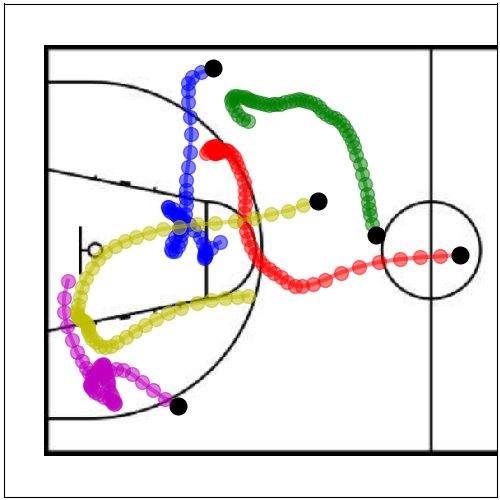
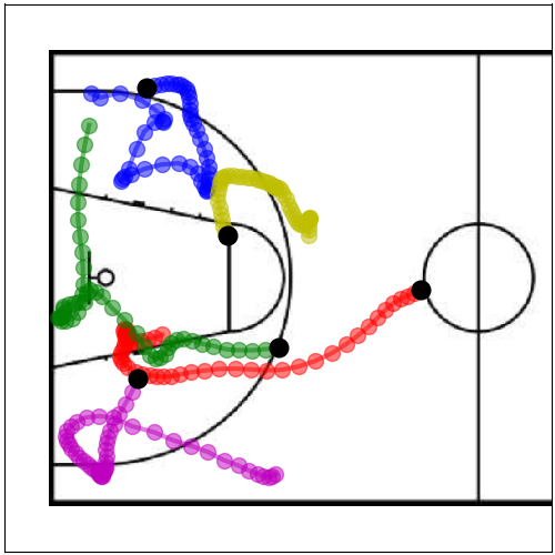
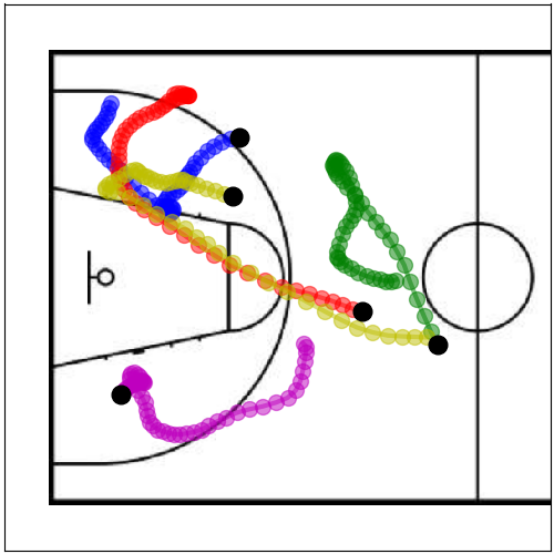
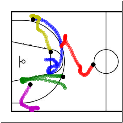
We let $d_{g}=d_{z}=32$. All RNNs are specified to be two-layer, 64-unit LSTMs and all MLPs use 256 hidden units. The generative model uses one 8-head MHA layer and the proposal uses two 8-head MHA layers. Each GNF uses an additional MHA layer shared by the functions $s(\cdot)$ and $t(\cdot)$. 4 SMC samples and a batch size of 64 are used in training. Eight selected rollouts from the trained model are visualized in Figure 3.

Figure 3: Selected rollouts from the trained model. Black dots represent the starting points.

Road traffic.

We let $d_{g}=d_{z}=8$. A 32-dimensional embedding for each sensor is jointly learned as a part of the vertex attribute. All RNNs are specified to be two-layer, 32-unit LSTMs and all MLPs use 64 hidden units. The generative model and the proposal both use two 8-head MHA layers. 3 SMC samples and a batch size of 16 are used in training.

A.4 Training

We optimize the VSMC bound estimated by the following SMC algorithm:

Algorithm 1 Estimate the VSMC bound $\mathcal{L}_{K}^{\text{SMC}}$

  Input: graph $\mathcal{G}$, observations $\mathbf{X}_{1:T}$, exogenous inputs $\mathbf{U}_{1:T}$

  Require: generative model $\{f_{\theta}^{g},f_{\theta}^{\star},g_{\theta}\}$, proposal $\{r_{\phi}^{g},r_{\phi}^{\star}\}$, number of particles $K$

  

  for $k=1\ldots K$ do

     Simulate $\mathbf{z}_{1,k}^{g}\sim r_{\phi}^{g}(\cdot|\mathcal{G},\mathbf{X}_{1},\mathbf{U}_{1})$

     Simulate $\mathbf{Z}_{1,k}\sim r_{\phi}^{\star}(\cdot|\mathbf{z}_{1,k}^{g},\mathcal{G},\mathbf{X}_{1},\mathbf{U}_{1})$

     Set $w_{1}^{k}=\frac{f_{\theta}^{g}(\mathbf{z}_{1,k}^{g})f_{\theta}^{\star}(\mathbf{Z}_{1,k}|\mathbf{z}_{1,k}^{g},\,\mathcal{G},\,\mathbf{U}_{1})\prod_{i=1}^{N}{g_{\theta}(\mathbf{x}_{1}^{(i)}|\mathbf{z}_{1,k}^{(i)},\,\mathbf{z}_{1,k}^{g},\,\ldots)}}{r_{\phi}^{g}(\mathbf{z}_{1,k}^{g}|\ldots)r_{\phi}^{\star}(\mathbf{Z}_{1,k}|\ldots)}$

  end for

  Initialize $\hat{\mathcal{L}}^{\text{SMC}}_{K}=\log{\sum_{k=1}^{K}{\nicefrac{{w_{1}^{k}}}{{K}}}}$

  

  for $t=2\ldots T$ do

     $\{\mathbf{z}_{<t,k}^{g},\mathbf{Z}_{<t,k}\}_{k=1}^{K}=\text{RESAMPLE}(\{\mathbf{z}_{<t,k}^{g},\mathbf{Z}_{<t,k},w_{t-1}^{k}\}_{k=1}^{K})$

     for $k=1\ldots K$ do

        Simulate $\mathbf{z}_{t,k}^{g}\sim r_{\phi}^{g}(\cdot|\mathbf{z}_{<t,k}^{g},\mathbf{Z}_{<t,k},\mathcal{G},\mathbf{X}_{\leq t},\mathbf{U}_{\leq t})$

        Simulate $\mathbf{Z}_{t,k}\sim r_{\phi}^{\star}(\cdot|\mathbf{z}_{\leq t,k}^{g},\mathbf{Z}_{<t,k},\mathcal{G},\mathbf{X}_{\leq t},\mathbf{U}_{\leq t})$

        Set $w_{t}^{k}=\frac{f_{\theta}^{g}(\mathbf{z}_{t,k}^{g}|\ldots)f_{\theta}^{\star}(\mathbf{Z}_{t,k}|\mathbf{z}_{\leq t,k}^{g},\,\mathbf{Z}_{<t,k},\,\ldots)\prod_{i=1}^{N}{g_{\theta}(\mathbf{x}_{t}^{(i)}|\mathbf{z}_{t,k}^{(i)},\,\mathbf{z}_{\leq t,k}^{g},\,\mathbf{Z}_{<t,k},\,\ldots)}}{r_{\phi}^{g}(\mathbf{z}_{t,k}^{g}|\ldots)r_{\phi}^{\star}(\mathbf{Z}_{t,k}|\ldots)}$

        Set $\mathbf{z}_{\leq t,k}^{g}=(\mathbf{z}_{<t,k}^{g},\mathbf{z}_{t,k}^{g})$, $\mathbf{Z}_{\leq t,k}=(\mathbf{Z}_{<t,k},\mathbf{Z}_{t,k})$

     end for

     Update $\hat{\mathcal{L}}^{\text{SMC}}_{K}=\hat{\mathcal{L}}^{\text{SMC}}_{K}+\log{\sum_{k=1}^{K}{\nicefrac{{w_{t}^{k}}}{{K}}}}$

  end for

  

  Output: $\hat{\mathcal{L}}^{\text{SMC}}_{K}$

In our model, dependencies on $\mathbf{z}_{<t,k}^{g}$ and $\mathbf{Z}_{<t,k}$ are provided through the compact RNN states $\mathbf{h}_{t,k}^{g}$ and $\mathbf{H}_{t,k}$. When GNFs are used in $f_{\theta}^{\star}$ and $r_{\phi}^{\star}$, density calculation and backpropagation are automatically handled by the TensorFlow Probability library.

To estimate the auxiliary objectives $\mathcal{L}_{1}^{\text{aux}}$ and $\mathcal{L}_{2}^{\text{aux}}$, we reuse the resampled unweighted particles $\{\{\mathbf{z}_{1:t,k}^{g},\mathbf{Z}_{1:t,k}\}_{k=1}^{K}\}_{t=1}^{T-1}$ generated by Algorithm 1 to form Monte Carlo estimations for them:

$$\hat{\mathcal{L}}_{1}^{\text{aux}}=\sum_{t=1}^{T-1}\sum_{i=1}^{N}\frac{1}{K}\log\frac{\lambda_{\psi,1}(\hat{\mathbf{z}}_{t,k}^{(i)},\mathbf{c}_{t}^{(i)})}{\sum_{\mathbf{c}\in\Omega_{t,i}}{\lambda_{\psi,1}(\hat{\mathbf{z}}_{t,k}^{(i)},\mathbf{c})}},\;\hat{\mathcal{L}}_{2}^{\text{aux}}=\sum_{t=1}^{T-1}\sum_{i=1}^{N}\frac{1}{K}\log\frac{\lambda_{\psi,2}(\hat{\mathbf{h}}_{t,k}^{(i)},\mathbf{c}_{t}^{(i)})}{\sum_{\mathbf{c}\in\Omega_{t,i}}{\lambda_{\psi,2}(\hat{\mathbf{h}}_{t,k}^{(i)},\mathbf{c})}}$$

where $\hat{\mathbf{z}}_{t,k}^{(i)}=[\mathbf{z}_{t,k}^{g},\mathbf{z}_{t,k}^{(i)}]$, $\hat{\mathbf{h}}_{t,k}^{(i)}=\text{MLP}_{\psi}(\sum_{j\neq i\,\wedge\,j\in\mathcal{N}_{i}^{-}}{\mathbf{h}_{t,k}^{(j)}})$, and $\Omega_{t,i}$ is a set that contains $\mathbf{c}_{t}^{(i)}$ and some negative samples selected from the future summaries of other vertices within the minibatch.

A.5 Graph Normalizing Flow

Figure 4: Visual illustration of a GNF. Multiple GNFs can be stacked together to achieve more expressive transformation.

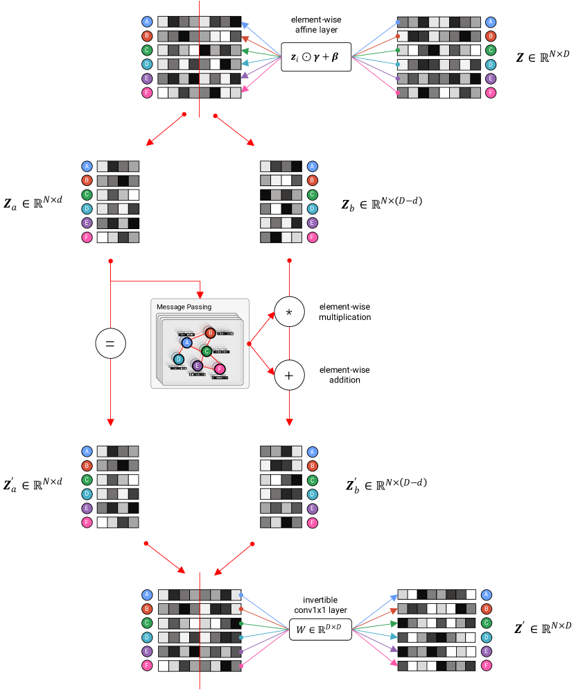
The element-wise affine layer is proposed by Kingma & Dhariwal (2018) for normalizing the activations. Its parameters $\bm{\gamma}\in\mathbb{R}^{D}$ and $\bm{\beta}\in\mathbb{R}^{D}$ are initialized such that the per-channel activations have roughly zero mean and unit variance at the beginning of training. The invertible linear transformation $\mathbf{W}\in\mathbb{R}^{D\times D}$ is parameterized using a QR decomposition Hoogeboom et al. (2019).

References

- Alahi et al. (2016) Alexandre Alahi, Kratarth Goel, Vignesh Ramanathan, Alexandre Robicquet, Li Fei-Fei, and Silvio Savarese. Social lstm: Human trajectory prediction in crowded spaces. In Proceedings of the IEEE Conference on Computer Vision and Pattern Recognition, 2016.
- Andrieu et al. (2010) Christophe Andrieu, Arnaud Doucet, and Roman Holenstein. Particle markov chain monte carlo methods. Journal of the Royal Statistical Society: Series B (Statistical Methodology), 72(3):269–342, 2010.
- Battaglia et al. (2016) Peter Battaglia, Razvan Pascanu, Matthew Lai, Danilo Jimenez Rezende, and koray kavukcuoglu. Interaction networks for learning about objects, relations and physics. In Advances in Neural Information Processing Systems 29. 2016.
- Battaglia et al. (2018) Peter W Battaglia, Jessica B Hamrick, Victor Bapst, Alvaro Sanchez-Gonzalez, Vinicius Zambaldi, Mateusz Malinowski, Andrea Tacchetti, David Raposo, Adam Santoro, Ryan Faulkner, et al. Relational inductive biases, deep learning, and graph networks. arXiv preprint arXiv:1806.01261, 2018.
- Bayer & Osendorfer (2014) Justin Bayer and Christian Osendorfer. Learning stochastic recurrent networks. arXiv preprint arXiv:1411.7610, 2014.
- Buesing et al. (2018) Lars Buesing, Theophane Weber, Sebastien Racaniere, SM Eslami, Danilo Rezende, David P Reichert, Fabio Viola, Frederic Besse, Karol Gregor, Demis Hassabis, et al. Learning and querying fast generative models for reinforcement learning. arXiv preprint arXiv:1802.03006, 2018.
- Chang et al. (2017) Michael Chang, Tomer Ullman, Antonio Torralba, and Joshua Tenenbaum. A compositional object-based approach to learning physical dynamics. In International Conference on Learning Representations. 2017.
- Chung et al. (2015) Junyoung Chung, Kyle Kastner, Laurent Dinh, Kratarth Goel, Aaron C Courville, and Yoshua Bengio. A recurrent latent variable model for sequential data. In Advances in Neural Information Processing Systems 28, 2015.
- Defferrard et al. (2016) Michaël Defferrard, Xavier Bresson, and Pierre Vandergheynst. Convolutional neural networks on graphs with fast localized spectral filtering. In Advances in Neural Information Processing Systems 29. 2016.
- Dillon et al. (2017) Joshua V Dillon, Ian Langmore, Dustin Tran, Eugene Brevdo, Srinivas Vasudevan, Dave Moore, Brian Patton, Alex Alemi, Matt Hoffman, and Rif A Saurous. Tensorflow distributions. arXiv preprint arXiv:1711.10604, 2017.
- Dinh et al. (2017) Laurent Dinh, Jascha Sohl-Dickstein, and Samy Bengio. Density estimation using real nvp. In International Conference on Learning Representations, 2017.
- Doucet & Johansen (2009) Arnaud Doucet and Adam M Johansen. A tutorial on particle filtering and smoothing: Fifteen years later. Handbook of Nonlinear Filtering, 2009.
- Duvenaud et al. (2015) David K Duvenaud, Dougal Maclaurin, Jorge Iparraguirre, Rafael Bombarell, Timothy Hirzel, Alan Aspuru-Guzik, and Ryan P Adams. Convolutional networks on graphs for learning molecular fingerprints. In Advances in Neural Information Processing Systems 28. 2015.
- Fraccaro (2018) Marco Fraccaro. Deep Latent Variable Models for Sequential Data. PhD thesis, 2018.
- Fraccaro et al. (2016) Marco Fraccaro, Søren Kaae Sø nderby, Ulrich Paquet, and Ole Winther. Sequential neural models with stochastic layers. In Advances in Neural Information Processing Systems 29, 2016.
- Fraccaro et al. (2017) Marco Fraccaro, Simon Kamronn, Ulrich Paquet, and Ole Winther. A disentangled recognition and nonlinear dynamics model for unsupervised learning. In Advances in Neural Information Processing Systems 30, 2017.
- Gilmer et al. (2017) Justin Gilmer, Samuel S. Schoenholz, Patrick F. Riley, Oriol Vinyals, and George E. Dahl. Neural message passing for quantum chemistry. In Proceedings of the International Conference on Machine Learning, 2017.
- Goodfellow et al. (2014) Ian Goodfellow, Jean Pouget-Abadie, Mehdi Mirza, Bing Xu, David Warde-Farley, Sherjil Ozair, Aaron Courville, and Yoshua Bengio. Generative adversarial nets. In Advances in Neural Information Processing Systems 27. 2014.
- Goyal et al. (2017) Anirudhand Goyal, Alessandro Sordoni, Marc-Alexandre Côté, Nan Rosemary Ke, and Yoshua Bengio. Z-forcing: Training stochastic recurrent networks. In Advances in Neural Information Processing Systems 30, 2017.
- Gregor et al. (2019) Karol Gregor, George Papamakarios, Frederic Besse, Lars Buesing, and Theophane Weber. Temporal difference variational auto-encoder. In International Conference on Learning Representations, 2019.
- Gu et al. (2015) Shixiang (Shane) Gu, Zoubin Ghahramani, and Richard E Turner. Neural adaptive sequential monte carlo. In Advances in Neural Information Processing Systems 28. 2015.
- Gupta et al. (2018) Agrim Gupta, Justin Johnson, Li Fei-Fei, Silvio Savarese, and Alexandre Alahi. Social gan: Socially acceptable trajectories with generative adversarial networks. In Proceedings of the IEEE Conference on Computer Vision and Pattern Recognition, 2018.
- Hafner et al. (2019) Danijar Hafner, Timothy Lillicrap, Ian Fischer, Ruben Villegas, David Ha, Honglak Lee, and James Davidson. Learning latent dynamics for planning from pixels. In Proceedings of the International Conference on Machine Learning, 2019.
- Hajiramezanali et al. (2019) Ehsan Hajiramezanali, Arman Hasanzadeh, Nick Duffield, Krishna R Narayanan, Mingyuan Zhou, and Xiaoning Qian. Variational graph recurrent neural networks. In Advances in Neural Information Processing Systems 32. 2019.
- Hamilton et al. (2017) Will Hamilton, Zhitao Ying, and Jure Leskovec. Inductive representation learning on large graphs. In Advances in Neural Information Processing Systems 30. 2017.
- He et al. (2016) Kaiming He, Xiangyu Zhang, Shaoqing Ren, and Jian Sun. Deep residual learning for image recognition. In Proceedings of the IEEE Conference on Computer Vision and Pattern Recognition, 2016.
- Hirt & Dellaportas (2019) Marcel Hirt and Petros Dellaportas. Scalable bayesian learning for state space models using variational inference with smc samplers. In Proceedings of the International Conference on Artificial Intelligence and Statistics, 2019.
- Hoogeboom et al. (2019) Emiel Hoogeboom, Rianne van den Berg, and Max Welling. Emerging convolutions for generative normalizing flows. In Proceedings of the International Conference on Machine Learning, 2019.
- Hoshen (2017) Yedid Hoshen. Vain: Attentional multi-agent predictive modeling. In Advances in Neural Information Processing Systems 30. 2017.
- Janner et al. (2019) Michael Janner, Sergey Levine, William T. Freeman, Joshua B. Tenenbaum, Chelsea Finn, and Jiajun Wu. Reasoning about physical interactions with object-centric models. In International Conference on Learning Representations, 2019.
- Kantas et al. (2015) Nikolas Kantas, Arnaud Doucet, Sumeetpal S Singh, Jan Maciejowski, Nicolas Chopin, et al. On particle methods for parameter estimation in state-space models. Statistical Science, 30(3):328–351, 2015.
- Karl et al. (2016) Maximilian Karl, Maximilian Soelch, Justin Bayer, and Patrick van der Smagt. Deep variational bayes filters: Unsupervised learning of state space models from raw data. In International Conference on Learning Representations. 2016.
- Ke et al. (2019) Nan Rosemary Ke, Amanpreet Singh, Ahmed Touati, Anirudh Goyal, Yoshua Bengio, Devi Parikh, and Dhruv Batra. Modeling the long term future in model-based reinforcement learning. In International Conference on Learning Representations, 2019.
- Kingma & Welling (2014) Diederik P Kingma and Max Welling. Auto-encoding variational bayes. In International Conference on Learning Representations. 2014.
- Kingma & Dhariwal (2018) Durk P Kingma and Prafulla Dhariwal. Glow: Generative flow with invertible 1x1 convolutions. In Advances in Neural Information Processing Systems 31. 2018.
- Kingma et al. (2016) Durk P Kingma, Tim Salimans, Rafal Jozefowicz, Xi Chen, Ilya Sutskever, and Max Welling. Improved variational inference with inverse autoregressive flow. In Advances in Neural Information Processing Systems 29. 2016.
- Kipf et al. (2018) Thomas Kipf, Ethan Fetaya, Kuan-Chieh Wang, Max Welling, and Richard Zemel. Neural relational inference for interacting systems. In Proceedings of the International Conference on Machine Learning, 2018.
- Kosaraju et al. (2019) Vineet Kosaraju, Amir Sadeghian, Roberto Martín-Martín, Ian Reid, S. Hamid Rezatofighi, and Silvio Savarese. Social-bigat: Multimodal trajectory forecasting using bicycle-gan and graph attention networks. In Advances in Neural Information Processing Systems 32. 2019.
- Kosiorek et al. (2018) Adam Kosiorek, Hyunjik Kim, Yee Whye Teh, and Ingmar Posner. Sequential attend, infer, repeat: Generative modelling of moving objects. In Advances in Neural Information Processing Systems 31. 2018.
- Krishnan et al. (2017) Rahul G Krishnan, Uri Shalit, and David Sontag. Structured inference networks for nonlinear state space models. In AAAI Conference on Artificial Intelligence, 2017.
- Le et al. (2018) Tuan Anh Le, Maximilian Igl, Tom Rainforth, Tom Jin, and Frank Wood. Auto-encoding sequential monte carlo. In International Conference on Learning Representations, 2018.
- Li et al. (2018) Yaguang Li, Rose Yu, Cyrus Shahabi, and Yan Liu. Diffusion convolutional recurrent neural network: Data-driven traffic forecasting. In International Conference on Learning Representations, 2018.
- Li et al. (2016) Yujia Li, Daniel Tarlow, Marc Brockschmidt, and Richard Zemel. Gated graph sequence neural networks. International Conference on Learning Representations, 2016.
- Li et al. (2019) Yunzhu Li, Jiajun Wu, Russ Tedrake, Joshua B. Tenenbaum, and Antonio Torralba. Learning particle dynamics for manipulating rigid bodies, deformable objects, and fluids. In International Conference on Learning Representations, 2019.
- Liu et al. (2019) Jenny Liu, Aviral Kumar, Jimmy Ba, Jamie Kiros, and Kevin Swersky. Graph normalizing flows. In Advances in Neural Information Processing Systems 32. 2019.
- Maddison et al. (2017) Chris J Maddison, John Lawson, George Tucker, Nicolas Heess, Mohammad Norouzi, Andriy Mnih, Arnaud Doucet, and Yee Teh. Filtering variational objectives. In Advances in Neural Information Processing Systems 30. 2017.
- Marino et al. (2018) Joseph Marino, Milan Cvitkovic, and Yisong Yue. A general method for amortizing variational filtering. In Advances in Neural Information Processing Systems 31. 2018.
- Maron et al. (2019) Haggai Maron, Heli Ben-Hamu, Nadav Shamir, and Yaron Lipman. Invariant and equivariant graph networks. In International Conference on Learning Representations, 2019.
- Mrowca et al. (2018) Damian Mrowca, Chengxu Zhuang, Elias Wang, Nick Haber, Li F Fei-Fei, Josh Tenenbaum, and Daniel L Yamins. Flexible neural representation for physics prediction. In Advances in Neural Information Processing Systems 31. 2018.
- Naesseth et al. (2019) C. A. Naesseth, F. Lindsten, and T. B. Schön. High-dimensional filtering using nested sequential monte carlo. IEEE Transactions on Signal Processing, 67(16):4177–4188, 2019.
- Naesseth et al. (2018) Christian Naesseth, Scott Linderman, Rajesh Ranganath, and David Blei. Variational sequential monte carlo. In Proceedings of the International Conference on Artificial Intelligence and Statistics, 2018.
- Oord et al. (2018) Aaron van den Oord, Yazhe Li, and Oriol Vinyals. Representation learning with contrastive predictive coding. arXiv preprint arXiv:1807.03748, 2018.
- Papamakarios et al. (2017) George Papamakarios, Theo Pavlakou, and Iain Murray. Masked autoregressive flow for density estimation. In Advances in Neural Information Processing Systems 30. 2017.
- Rezende & Mohamed (2015) Danilo Rezende and Shakir Mohamed. Variational inference with normalizing flows. In Proceedings of the International Conference on Machine Learning, 2015.
- Rhinehart et al. (2019) Nicholas Rhinehart, Rowan McAllister, Kris Kitani, and Sergey Levine. Precog: Prediction conditioned on goals in visual multi-agent settings. In The IEEE International Conference on Computer Vision, 2019.
- Sanchez-Gonzalez et al. (2018) Alvaro Sanchez-Gonzalez, Nicolas Heess, Jost Tobias Springenberg, Josh Merel, Martin Riedmiller, Raia Hadsell, and Peter Battaglia. Graph networks as learnable physics engines for inference and control. In Proceedings of the International Conference on Machine Learning, 2018.
- Scarselli et al. (2009) Franco Scarselli, Marco Gori, Ah Chung Tsoi, Markus Hagenbuchner, and Gabriele Monfardini. The graph neural network model. IEEE Transactions on Neural Networks, 20(1):61–80, 2009.
- Sun et al. (2019) Chen Sun, Per Karlsson, Jiajun Wu, Joshua B Tenenbaum, and Kevin Murphy. Stochastic prediction of multi-agent interactions from partial observations. In International Conference on Learning Representations, 2019.
- Sutskever et al. (2014) Ilya Sutskever, Oriol Vinyals, and Quoc V Le. Sequence to sequence learning with neural networks. In Advances in Neural Information Processing Systems 27. 2014.
- Tacchetti et al. (2019) Andrea Tacchetti, H. Francis Song, Pedro A. M. Mediano, Vinicius Zambaldi, János Kramár, Neil C. Rabinowitz, Thore Graepel, Matthew Botvinick, and Peter W. Battaglia. Relational forward models for multi-agent learning. In International Conference on Learning Representations, 2019.
- Tang & Salakhutdinov (2019) Yichuan Charlie Tang and Ruslan Salakhutdinov. Multiple futures prediction. In Advances in Neural Information Processing Systems 32. 2019.
- van Steenkiste et al. (2018) Sjoerd van Steenkiste, Michael Chang, Klaus Greff, and Jürgen Schmidhuber. Relational neural expectation maximization: Unsupervised discovery of objects and their interactions. In International Conference on Learning Representations, 2018.
- Vaswani et al. (2017) Ashish Vaswani, Noam Shazeer, Niki Parmar, Jakob Uszkoreit, Llion Jones, Aidan N Gomez, Ł ukasz Kaiser, and Illia Polosukhin. Attention is all you need. In Advances in Neural Information Processing Systems 30. 2017.
- Veličković et al. (2018) Petar Veličković, Guillem Cucurull, Arantxa Casanova, Adriana Romero, Pietro Liò, and Yoshua Bengio. Graph attention networks. In International Conference on Learning Representations, 2018.
- Watters et al. (2017) Nicholas Watters, Daniel Zoran, Theophane Weber, Peter Battaglia, Razvan Pascanu, and Andrea Tacchetti. Visual interaction networks: Learning a physics simulator from video. In Advances in Neural Information Processing Systems 30. 2017.
- Xu et al. (2019) Keyulu Xu, Weihua Hu, Jure Leskovec, and Stefanie Jegelka. How powerful are graph neural networks? In International Conference on Learning Representations, 2019.
- Yang et al. (2018) Zhilin Yang, Zihang Dai, Ruslan Salakhutdinov, and William W. Cohen. Breaking the softmax bottleneck: a high-rank RNN language model. In International Conference on Learning Representations, 2018.
- Yeh et al. (2019) Raymond A. Yeh, Alexander G. Schwing, Jonathan Huang, and Kevin Murphy. Diverse generation for multi-agent sports games. In Proceedings of the IEEE Conference on Computer Vision and Pattern Recognition, 2019.
- Zhan et al. (2019) Eric Zhan, Stephan Zheng, Yisong Yue, Long Sha, and Patrick Lucey. Generating multi-agent trajectories using programmatic weak supervision. In International Conference on Learning Representations, 2019.
- Zhang et al. (2018) Jiani Zhang, Xingjian Shi, Junyuan Xie, Hao Ma, Irwin King, and Dit-Yan Yeung. Gaan: Gated attention networks for learning on large and spatiotemporal graphs. In Conference on Uncertainty in Artificial Intelligence, 2018.
- Zheng et al. (2017) Xun Zheng, Manzil Zaheer, Amr Ahmed, Yuan Wang, Eric P Xing, and Alexander J Smola. State space lstm models with particle mcmc inference. arXiv preprint arXiv:1711.11179, 2017.