Alternate bearing and possibile long-range communication of Olea europaea

Abstract

Spatio-temporal analysis typically performed in horticulture and in statistical physics reveals persistent correlations of olive yields which range depend on the size of the averaging regions. Mapping spatially correlated regions unveils areas which resemble historical spread of Olea europaea. These yield patterns are remarkable given the intensive nature of modern agriculture, and cannot be attributed to weather or pollen indices due to inability of these variables to properly predict yields, and their different correlation patterns. Long-range correlations between yields of olive trees may indicate long-range communications among trees.

July 28, 2018

1 Introduction

Another problem of evaluation, useful when discussing alternation, seems to have not been quantitatively approached: synchronization of different plants within a single orchard or of different orchards within a single region. Such an attempt would provide a basis to evaluate to what extent external factors (common to a grove, an area, etc.) are dominant as against internal factors of trees or factors common to a restricted area, such as microclimate, soil-rootstock-cultivar relationships, etc.

[1], p. 131

About four decades have passed since the above request for a quantitative model of alternate bearing was written, these decades saw an intensifying research into the origin and control of alternate bearing - a phenomenon where crops alternate, year after year, in an approximate ’year on - year off’ but otherwise seemingly random fashion. Olive trees, with their praised fruits, and relatively detailed historical records, are similar to many other plants in this regard. A year of abundance is usually followed by a year of low crops, and vice versa, but not necessarily, and not everywhere. Alterations extend over at least 5-6 orders of magnitude in space, ranging from a single olive tree (leaving aside the branch-to-branch alterations) to scales of hundreds if not thousands of kilometers, at times - across a body of water. This phenomenon is known to resist human control which routinely includes such drastic measures as cultivation of young trees, aggressive annual pruning, planting trees in a optimized dense grid [2], and a wide spectrum of biochemical applications.

On one side, truly biannual alterations could only be in one of two phases (on or off for a given tree in a given year), which would make quickly decaying random spatial patterns after spatial averaging were it not for synchronized regions which may extend over hundreds of kilometers, and include geographically separated trees. On the other side, there is no known clear predictor of yield at large scales (except, obviously, the yield itself), while there is no shortage of factors considered, [3]. Among external factors, attempts to use pollen [4], [5], and weather-related variables for crop predictions are repeatedly revisited [6], [7], [8], [9], [10].

Below, starting with data analysis, we briefly present a comparison of different correlation measures which either have been of could be of interest regarding alternate bearing, and argue that these measures cannot be explained endogenously, suggesting a potential long-range communication between olive trees.

2 Spatio-temporal correlations in olive plantations

In this section we will address the correlations of the surface density of the annual olive crops. This variable is termed ’yield’ in agriculture. The time scale $t$, for yield, $Y_{t}(x)$ is discrete (integer indices $t$, $t+1$, $t+2$, … refer to years), while $x$ are spatial scales. Historical data are seldom available at the sub-tree level, but tree-level data are sometimes available at research institutions, and public data can be found at county, province and country level and can be obtained from government or non-for-profit sources and from The Statistics Division of The United Nations [11].

We first perform a study of the type usually done in statistical physics [12]. Since plants are inherently Malthusian systems, we consider correlations of normalized logarithmic yields,

$$y_{t}(x)=\frac{1}{\sigma(x)}\left[\log Y_{t}(x)-\langle\log Y(x)\rangle\right],$$ (1)

where $\langle...\rangle$ is an average over multiple years (hence, no time index), and $\sigma(x)$ is the standard deviation of the logarithm (again, no time index). The average

$$\rho_{1}(t^{\prime}-t)=\langle y_{t}(x)y_{t^{\prime}}(x)\rangle,$$ (2)

is then the correlation coefficient over the lag of $t^{\prime}-t$ years, called the autocorrelation below. Here $t^{\prime}-t=1,2,...$.

Location	Years	$\rho_{1}(1)$	$L$, km	$B$	$I_{B}$	$S$	$I_{S}$
Montsià	2008-2013	$-0.66\pm 0.23$	n/a	1	0.28	n/a	n/a
Málaga	1999-2013	$-0.55\pm 0.18$	n/a	0.77	0.17	n/a	n/a
Tarragona	2006-2013	$-0.02\pm 0.35$	67	0.83	0.15	0.5 to 1	0.37 to 0.45
Lleida	2006-2013	$-0.08\pm 0.35$	248	0.5	0.18	0.5 to 1	0.31 to 0.36
Andalucia	1999-2013	$-0.31\pm 0.23$	189	0.61	0.18	0.5 to 1	0.20 to 0.32
Spain	1999-2013	$-0.36\pm 0.16$	n/a	0.5	0.11	n/a	n/a
World	1999-2013	$-0.28\pm 0.24$	603	0.52	0.03	0.52 to 0.55	0.40 to 0.57

Table 1: Different measures of alterations. $\rho_{1}$ is the yield one-year autocorrelation, (2), $L$ is the correlation length (3), $B$ - biennuality (5), $I_{B}$ - intensity (6), $S$ - synchronization (7), $I_{S}$ - relative amplitude of spatial fluctuations (8). At the locations, where we did not have subdivision data available, spatial indices are given as ’n/a’. Synchronicity, $S$, depends on time, and the minimum and maximum values are given. Málaga is chosen over Jaén because the latter determines the entire Andalusia, and its values are close to Andalusian ones.

A certain degree of alternation is observed in the time series of yield, and one can see in Table 1 that on average one-year autocorrelations are negative, $\rho_{1}(1)<0$. The residual noise is not small, and phases of biennual patterns change in what seems to be a random fashion.

The average

$$\rho_{2}(x^{\prime}-x)=\langle y_{t}(x)y_{t}(x^{\prime})\rangle$$ (3)

is a spatial correlation coefficient over the distance $x^{\prime}-x$. An important property of this correlation is its decay, which we will model by means of a single correlation length,

$$\rho_{2}(x)\propto\exp\left(-x^{2}/L^{2}\right).$$ (4)

Remarkably, the fitted correlation length, $L$, is found to depend on the dataset scale, see Fig1. For the province of Tarragona it is 67 km, for Andalusia - 189 km, and for the Europe/Africa/Middle East dataset it is 603 km, see also Table 1. The largest of these correlations lengths is comparable to the latitudinal span of The Mediterranean Sea.

Figure 1: Decay of spatial correlations $\rho_{2}$ at different scales. $x$-axis is distance in kilometers in all subplots. Vertical lines show error bars. Red lines are fits using Eq (3) with correlation length $L$ given below each subplots.

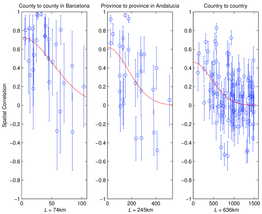
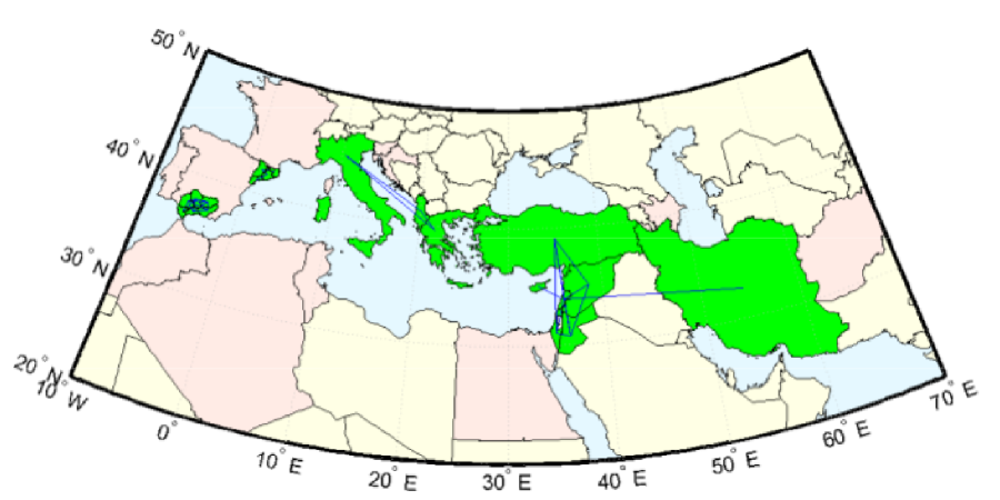
Scale-dependent spatial correlations of olive yields indicate a presence of hierarchical spatial structures. One should then expect that there are subsets of locations where correlations decay much slower with distance, as compared to what (3) prescribes, and subsets which decay much faster. And indeed, further investigation shows that correlations decay slower with distance in Lleida province of Catalonia than in Tarragona, and that Córdoba, Granada, Jaén, and Málaga act as a single entity in Andalusia, and the same can be said, for example, about olive yields in Turkey, Syria, Lebanon, Cyprus, et cetera. It is then of interest to obtain a correlation map, which gives a visual representation of these connections, see Fig 2.

Figure 2: Green and pink countries submitted official reports to FAOSTAT for at least a decade. The countries, which are pairwise correlated with $\rho_{2}>1/2$, are colored green and connected by straight blue lines. The entire countries are colored (even if their olive plantations are far from being uniform within country’s borders). The correlated countries form two clusters. Italy, Albania and Greece form one, and seven countries in the Middle East form another cluster. In Spain we show a province-level cluster in Catalonia and Andalusia. We do not have data for other provinces in Spain.

3 Exogenous yield predictors

A large number of factors which are exogenous to olive trees have been considered as yield predictors. These factors include weather (namely, temperature, humidity and precipitation) and solar irradiation. As these factors are themselves time-dependent, various filtered sums have been suggested as yield predictors [6], [7], [8], [9], [10]. In addition the significance of olive pollen has been recognized, [4], [5]. A belief that there might exist a very detailed weather-related predictor, along the lines of climate definitions and cluster analysis is persistent due to complexity of weather records. The following paragraph is taken from [10], “The meteorological variables considered in the present study were: monthly average of maximum and minimum temperatures (^∘C) and relative humidity (%), monthly accumulated precipitation (mm) and evapotranspiration (mm day–1), summer period (21st of June to 21st of September) accumulated mean temperature (^∘C) and accumulated precipitation (mm), and accumulated precipitation since the pre-flowering start date (end of March) until the peak pollination day (mm).”

Indeed, the scales of the largest clusters in Fig2 are comparable to correlation lengths for monthly averages of weather variables used in climate definitions. Nevertheless, the maps of spatial correlations of pollen, which reflect wind patterns, and other weather-based variables look quite different from Fig 2 (see below).

Since the yield time series which are regressed on these external factors are relatively short (they usually cover a couple of decades), it is always possible to find a meteorological candidate for yield regression, especially using filtered variables (such as a variable exceeding an optimized threshold). While the original findings of Hartmann and Porlingis [6] have been verified on numerous occasions, it is important to have sufficient out-of-sample analysis to avoid statistical overfitting.

The overall situation with using weather for explaining olive yields could be summarized as follows. While the weather and pollen indices continue to evolve to ’explain’ most recent data, the spatial correlations of the proposed exogenous indices do not reflect the same for the yields. At the same time, the overall existence of exogenous explanation is not questioned.

The yield correlation maps, however, resemble those of the olive tree varieties. Namely, correlation maps at the lowest level have resemblance to local olive varieties, while Fig2 which shows the largest scale considered here resembles the three historical ’inoculation waves’ of the olive tree expansion in the Mediterranean [13], based on genetic analysis.

4 Bienniality-intensity indices for alternate bearing

Horticulturists do not consider temporal or spatial correlations introduced above. Instead, they rely on frequency (known as $B$, for ’biennuality’) and severity (known as $I$, for ’intensity’) of alterations, defined as [1]

$$B =\frac{1}{n-2}\sum_{t=2}^{n-1}{\rm sign}\left(Y_{t+1}-Y_{t}\right){\rm sign}\left(Y_{t}-Y_{t-1}\right),$$ (5)

$$I_{B} =\frac{1}{n-1}\sum_{t=2}^{n}\frac{|Y_{t}-Y_{t-1}|}{Y_{t}+Y_{t-1}}$$ (6)

Bienniality indicates how frequently a trend changes, while intensity evaluates relative amplitudes of ’swings’. Both quantities supersede correlator (2) which origin is in gaussian (i.e. normal) statistics. On the other side, bienniality specifically focuses on two-year periods, while many olive plantations display more complex patterns (e.g. Jaén in 1999-2006 had a triennial alternation, rather than biennial). Both quantities have their analogs in terms of spatial correlations. Their spatial frequency is accessed through the ’synchronization’ parameter

$$S=\frac{1}{2}+\left|\frac{1}{2A}\sum_{x}{\hskip 1.8063pt}{\rm sign}\left[Y_{t}(x)-Y_{t-1}(x)\right]\right|,$$ (7)

which measures relative excess of trend increase or decrease in a given area. The value $S=0.5$ corresponds to complete randomization, while $S=1$ is full synchronization. We have not seen a measure of the amplitude of spatial fluctuations (an analog of the intensity above) to be considered in horticultural literature, as it is not an exclusive measure of alternative bearing. An index of relative spatial fluctuations can be defined as

$$I_{S}=\frac{1}{A^{2}}\sum_{x,x^{\prime}}{\hskip 1.8063pt}\frac{|Y_{t}(x)-Y_{t}(x^{\prime})|}{Y_{t}(x)+Y_{t}(x^{\prime})}.$$ (8)

Examples of numerical evaluation of these parameters can be found in Table 1. One can see that coarse-graining non only leads to decreasing of absolute values of one-year autocorrelation, $\rho_{1}(1)$, but also (i) the biennuality, $B$, is similarly suppressed, while remaining positive, (ii) the intensity of alternations, $I_{B}$, consistently diminishes with a characteristic distance of $10^{3}$ km, (iii) the spatial synchronization, $S$, of fluctuations becomes small only at the global level (Lleida or Andalusia, represented by counties, could still have $S=1$), and (iv) the index of relative spatial fluctuations, $I_{S}$, remains large at any level.

Thus, the alternate bearing can be averaged over, but it takes an effort: several decades in time and global spatial scales. In other words, for the data in Table 1 the alternate bearing can be found on all spatial scales.

5 Alternate bearing at a grove level

Data for an experimental grove, where different rootstocks are used, and trees are cared for in the same fashion as in agriculture, are particularly valuable, since they might contain detailed information about alternate bearing. These data require a considerable dedication: one has to maintain experimental groves for decades (IRTA).

The trees in the grove were arranged in a rectangle on a square grid: 10 blocks, 11 trees per block.

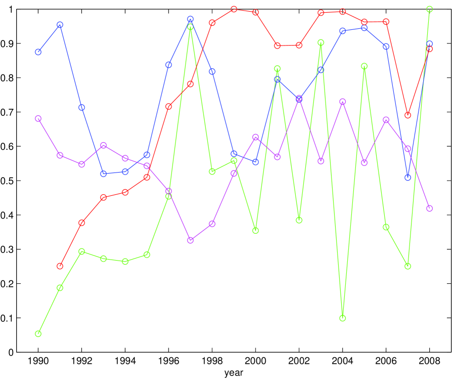
The overall behavior of the grove yield is shown in Fig 3. During the first 4 years of bearing (1989-1992, where 1989 is not shown), young trees grew exponentially in size and gave increasing yields, while their spatial synchronization, $I_{S}$, reached maximum in 1990, temporal synchronization, $S$ reached maximum in 1991, and yield, $Y_{t}$ reached maximum in 1992, accompanied by a decrease in both $S$ and $I_{S}$. Then, in 1993-1997 we have a consolidation phase, in response to increasing pruning, where synchronization in time is fully recovered as soon as pruning eased in 1996, while synchronization is space plunged to its minimum, allowing trees a semi-individualistic freerun. The yields reached a maximum in 1997 and were again pruned (c.f. the red line). In response to pruning, alternate bearing was fully developed by year 1999 with large negative autocorrelation $\rho_{1}(1)=-0.8$, and the grove entered an alternating regime where synchronization in time remained high, and synchronization is space was alternating out-of-phase with the yield (high $Y_{t}$ corresponded to lower $I_{S}$). In year 2007 trees were severely pruned, and it was accompanied by a phase shift of alternate bearing: year 2008 is the first even calendar year with a high yield. Overall there is a clear connection between alternate bearing and pruning: pruned olive trees enter a consolidation stage, regroup and re-synchronize in space to produce high yield in the year $t+1$ following excessive pruning in year $t$.

Figure 3: Time series of normalized net yield (rescaled to maximal yield ever observed) - green, synchronization parameter, $S$, - blue and spatial synchronization, $I_{B}$, - magenta, and normalized tree volume - red.

To understand whether yield synchronization is a collective phenomenon we comparatively time traced the behavior of the individual trees with maximal yields. For every two consecutive years, beginning with year 1990, a tree with the highest yield was selected, and its yield time series were plotted jointly with that of a tree which had the highest yield in the subsequent year (beginning with 1991, respectively). In Fig 4 we show subsequent synchronization of such consecutive leaders. As one can see, in many cases it took about two years for ex-leaders to synchronize in terms of alternate bearing. Some pairs (i.e. 1998/1999) did not subsequently synchronize, however in such infrequent cases the yield of one of the leaders subsequently declined. This may indicate that synchronization represents a healthy behavior. Some pairs (i.e. 2004/2005) were already synchronized even while being leaders in subsequent years. Interestingly, a minority subset of trees can always be identified which experiences alternate bearing out-of-phase with the majority. The lifetime of this out-of-phase alternate bearing does not exceed a couple of years, when the participating minority trees rejoin the quorum, while few new majority trees may join the out-of-phase minority. The out-of-phase alternate bearing may be used by the tree community for exploration of ’predators’ appearance during the majority off-years, and whether it is beneficial to switch to the opposite on-off phase instead.

Figure 4: Synchronization of leaders in two subsequent years. The blue circle is the maximal yield in a given year $t$, and blue line connects yields of that ’blue’ tree in all other years. The magenta circle is the maximal yield in the following year, $t+1$, and magenta line connects yields of that ’magenta’ tree in all other years. The $x$-axis is calendar years, and $y$-axis is yield in kilograms.

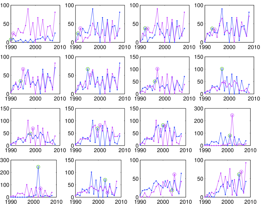
Fig 4 shows that synchronization is reestablished in majority of cases, and it is not, therefore, reducible to external factors. Indeed, if a particular winter chilling were to lead to an increased yield in a given year (say, year 1997 when the alternating pattern started), this cannot explain why leaders of the consecutive subsequent years had any incentive first to appear and then to re-synchronize with the majority. While external factors, such as winter chilling, are significant, they cannot substitute for the drivers of self-regulation.

Since Fig 4 only accounts for leaders, it is indicative of synchronization affecting the cases of maximal severity. It is even more instructive to see what happens to frequency of participation in the majority and minority of trees experiencing alternate bearing. With this in mind in Fig 5 we plotted the number of trees in both groups, along with the number of trees in transition between majority and minority and vice versa.

Figure 5: Top subplot. Number of trees participating in the majority group having either ’on’ year ($Y_{t}>Y_{t-1}$ and $Y_{t}>Y_{t+1}$) or ’off’ year ($Y_{t}<Y_{t-1}$ and $Y_{t}<Y_{t+1}$) is given by the green line, minority group - having the opposite year - is given by red line, trees which were members of the majority group and ended up as minority 2 years later are shown in cyan, and minority group trees synchronized with the majority are shown in magenta. Bottom subplot. The fractions obtained by dividing trees in transition to the total number of trees in the group they started from. In year $t=1993$ all trees had a yield increase, $Y_{t-1}<Y_{t}<Y_{t+1}$, so that this year cannot be classified as either ’on’ or ’off’ year for any tree.

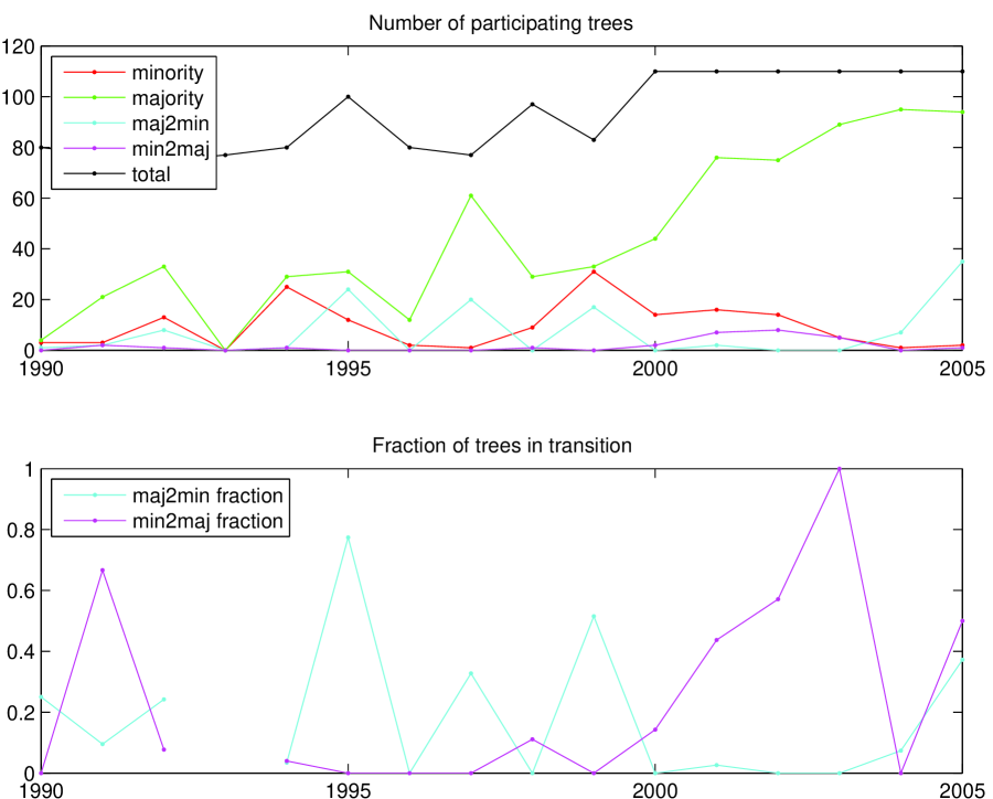
As one can see, the grove first maintains a comparable number of trees in both majority and minority groups (in terms of ’on/off’ years), and most trees do not participate in either group. Beginning with year 1997, when volume reduction due to pruning was (sufficiently?) large, the majority group for the first time reaches half of the grove, then the minority is given a chance to increase, but none of these adjustments helped to reduce pruning, and the majority is given a chance to approach $\leavevmode\nobreak\ 85\%$ of the trees. When even this does not help, in 2007, following intensive pruning, a switch to minority ’on/off’ pattern is performed by the entire grove skipping one ’on’ year, accumulating resources, and reaching the highest net yield ever in 2008.

In terms of spatial synchronization we did not observe any persistent spatial patterns. Synchronized trees seemed to occupy random slots, and so did out-of-phase trees. In view of high synchronization, this implies that the communication between the trees is long-ranged, since, for the randomness to be produced, every tree had to have information at least about the average state of the entire grove if not about every other tree in the grove. The mechanism of this long-ranged communication(s) remains to be identified. Note that this mechanism is not reducible to interaction via pollen (which is known to be correlated with yield, see above), since fruit bearing requires considerable resources to be accumulated in advance. Moreover, in view of the complex multistage phenological process unfolding during flowering and fruit bearing, any synchronization mechanism has to operate at least on multiple occasions if not continuously.

We conclude that alternate bearing is a collective phenomenon, accompanied by syn-chro-ni-za-tion in time, and alternate synchronization in space. Collective strategies, followed by the grove, are complex and show a feedback to pruning.

6 Conclusion

Spatial synchronization of alternative bearing is usually attributed to exogenous factors, such as pollen or weather indices. We find that the yield correlations do not follow the correlations of the ’explanatory’ pollen or weather variables. The observed synchronization in crop yields, which takes many months for trees to bear, is much stronger than what can be explained by pollen or weather. Given that trees are adaptive at all stages of their cycle, any persistent long-term, long-range synchronization requires similar and very frequent if not continuous communication. Given that mature olives still exist in the region [14], we suggest to consider whether humans interact with a plant organism of the size comparable to the Mediterranean scales, exceeding the so-called ’Pando’ organism of 43.6 ha of aspen trees [15]. Note than inside the Pando organism one also finds more than one genetic variate even among aspens.

7 Acknowledgment

The authors are most grateful to colleagues at IRTA (Institute of Agrifood Research and Technology, Generalitat de Catalunya, Spain) for access to experimental data on olive groves.

References

- [1] S.P. Monselise and E.E. Goldschmidt. Alternate bearing in fruit trees. Hortic Rev, 4:128–173, 1982.
- [2] J Tous, A Romero, J Plana, and F Baiges. Planting density trial with ‘Arbequina’ olive cultivar in Catalonia (Spain). In III International Symposium on Olive Growing 474, pages 177–180, 1997.
- [3] Shimon Lavee. Biennial bearing in olive (Olea europaea l.). In Annales Ser His Nat, volume 17, pages 101–112, 2007.
- [4] Marta Recio, Baltasar Cabezudo, M Mar Trigo, and F Javier Toro. Olea europaea pollen in the atmosphere of Málaga (S. Spain) and its relationship with meteorological parameters. Grana, 35(5):308–313, 1996.
- [5] Andrea Mazzeo, Marino Palasciano, Alessandra Gallotta, Salvatore Camposeo, Andrea Pacifico, and Giuseppe Ferrara. Amount and quality of pollen grains in four olive (Olea europaea L.) cultivars as affected by ‘on’and ‘off’ years. Scientia Horticulturae, 170:89–93, 2014.
- [6] H. T. Hartmann and I. Porlingis. Effect of different amounts of winter chilling on fruitfulness of several olive varieties. Botanical Gazette, 119(2):102–104, 1957.
- [7] Luis Rallo, P Torreno, A Vargas, and J Alvarado. Dormancy and alternate bearing in olive. In II International Symposium on Olive Growing 356, pages 127–136, 1993.
- [8] Marco Fornaciari, Fabio Orlandi, and Bruno Romano. Yield forecasting for olive trees. Agronomy Journal, 97(6):1537–1542, 2005.
- [9] C Galán, H García-Mozo, L Vázquez, L Ruiz, C Díaz De La Guardia, and E Domínguez-Vilches. Modeling olive crop yield in Andalusia, Spain. Agronomy Journal, 100(1):98–104, 2008.
- [10] F. Aguilera and L.Ruiz-Valenzuela. Forecasting olive crop yields based on long-term aerobiological data series and bioclimatic conditions for the southern Iberian peninsula. Spanish Journal of Agricultural Research, 12(1):215–224, 2014.
- [11] FAOSTAT. Food and Agriculture Organization of The United Nations, Statistics Division, Accessed on November 19, 2014, http://faostat3.fao.org/home/E, 2014.
- [12] L.D. Landau and E.M. Lifshitz. Fluid Mechanics, Second Edition: Volume 6 (Course of Theoretical Physics). Reed Elsevier, 2000.
- [13] G Besnard, B Khadari, M Navascués, M Fernández-Mazuecos, Ahmed El Bakkali, N Arrigo, D Baali-Cherif, V Brunini-Bronzini de Caraffa, S Santoni, P Vargas, et al. The complex history of the olive tree: from Late Quaternary diversification of Mediterranean lineages to primary domestication in the northern Levant. Proceedings of the Royal Society B: Biological Sciences, 280(1756):20122833, 2013.
- [14] Roselyne Lumaret and Noureddine Ouazzani. Plant genetics: Ancient wild olives in Mediterranean forests. Nature, 413(6857):700, 2001.
- [15] Jennifer DeWoody, Carol A Rowe, Valerie D Hipkins, and Karen E Mock. ”Pando” lives: molecular genetic evidence of a giant aspen clone in central Utah. Western North American Naturalist, 68(4):493–498, 2008.