Identification and nonlinearity compensation of hysteresis using NARX models

Abstract

This paper deals with two problems: the identification and compensation of hysteresis nonlinearity in dynamical systems using nonlinear polynomial autoregressive models with exogenous inputs (NARX). First, based on gray-box identification techniques, some constraints on the structure and parameters of NARX models are proposed to ensure that the identified models display a key-feature of hysteresis. In addition, a more general framework is developed to explain how hysteresis occurs in such models. Second, two strategies to design hysteresis compensators are presented. In one strategy the compensation law is obtained through simple algebraic manipulations performed on the identified models. It has been found that the compensators based on gray-box models outperform the cases with models identified using black-box techniques. In the second strategy, the compensation law is directly identified from the data. Both numerical and experimental results are presented to illustrate the efficiency of the proposed procedures.

, , and

• December 2019

Keywords: Hysteresis, gray-box identification, compensation of nonlinearities, NARX model

1 Introduction

Hysteresis is a nonlinear behavior that is present in several systems and devices. It is commonly related to the phenomena of ferromagnetism, plasticity, and friction, among others [1]. Some examples include mechanical, electronic and biomedical systems, as well as sensors and actuators such as magneto-rheological dampers, piezoelectric actuators and pneumatic control valves [2, 3, 4]. An intrinsic feature of such systems is the memory effect, meaning that their output depends on the history of the corresponding input.

In addition to the memory effect, the literature provides different definitions and conditions to distinguish such systems and characterize the hysteretic behavior. In some cases, the occurrence of hysteresis has been associated with the existence of several equilibrium points whenever these systems are subject to a constant [5] or time-varying [6] input signal. Additionally, hysteresis has also been defined as a hard nonlinearity that depends on the magnitude and rate of the input signal. These aspects can pose various performance limitations if not properly taken into account during the control design [7, 3]. Hence, a common goal is to attenuate the hysteretic behavior of the system [8, 9, 10].

In many approaches, the compensation of hysteresis starts with obtaining a suitable model. In the literature, several hysteresis models have been proposed based on phenomenological, black-box and gray-box modeling approaches.

In the realm of models based on first principles, important contributions have been made based on differential equations and operators [11], such as the Bouc-Wen model [12], the Duhem model [13], the Preisach model [14] and the Prandtl-Ishlinskii operator [15]. These models have been widely used to predict the hysteresis behavior due to their ability to describe a variety of hysteresis loops that resemble the proprieties of a wide class of real nonlinear hysteretic systems [16]. Besides, such models are known to be challenging for system identification techniques [17]. Apart from the computational effort required in the identification of phenomenological models, their application in the design of compensators is somewhat limited due to their structural complexity [4, 11].

Black-box modeling does not rely on prior knowledge about the system [18, 19, 20]. Unfortunately, relevant features that should be present in a model to reproduce hysteresis and an appropriate structure for designing compensators are not ensured by black-box techniques. Hence, the search for models that have specific features, that are accurate and that have a suitable structure for designing compensators remains an open problem.

Models obtained using gray-box techniques can be tailored to reproduce specific relevant features [21]. In this context, nonlinear autoregressive with exogenous inputs (NARX) models are considered a convenient choice due to their ability to predict a wide class of nonlinear behaviors [22, 23]. Another interesting feature is the structural flexibility of such models. Therefore, enforcing constraints on the model structure (e.g., in order to make it suitable for designing compensators) does not drastically affect its predictive ability [24]. Despite these promising aspects, the literature on this approach for modeling and compensating of hysteretic systems is scarce [25, 26, 27, 28, 6, 29].

In this sense, an important step in modeling the hysteresis nonlinearity was advanced in [6], in which sufficient conditions are presented for NARX models to display a hysteresis loop when subject to a certain class of input signals. The concept of a bounding structure ${\cal H}$ formed by sets of stable equilibria and its implication on the existence of the hysteresis loop in the identified models has also introduced in [6]. However, for more general cases, this concept and conditions need to be adapted. For instance, the conditions proposed in [6] are not sufficient to ensure the existence of several equilibrium points at steady-state [30, 5]. Also, the concept of bounding structure is limited to cases in which the sets of equilibria that form this structure are stable. Recently, a NARX model was identified for an experimental electronic circuit with hysteresis [29]. In this paper, we will propose ways to overcome some shortcomings pointed out in the aforementioned references and a more general framework will be put forward to explain how hysteresis takes place in identified models.

The main contributions of this work are: the proposition of a specific parameter constraint that ensures reproducing a key-feature of hysteresis through identified NARX models. A framework is put forward to explain how the hysteresis loop results from an interplay of attracting and repelling regions in the input-output plane. Moreover, some structural specifications are enforced during the identification procedure in such a way that the identified NARX model can be effectively used to mitigate the hysteresis nonlinearity. Hence, two model-based compensation strategies are introduced. In the first the compensation law is obtained through simple algebraic manipulations performed on the identified models. It has been found that the compensators based on gray-box models outperform the cases with models identified using black-box techniques. In the second strategy, the compensation law is directly identified from the data.

This work is organized as follows. Section 2 presents the background. A constraint to ensure hysteresis in the identified models and a framework for understanding how the hysteresis loop is formed are provided in section 3. Based on NARX models, two strategies to design compensators are detailed in section 4. The numerical and experimental results for the model identification and the compensator design are, respectively, given in sections 5 and 6. Section 7 presents the concluding remarks.

2 Background

A NARX model can be represented as [22]:

$$y_{k}=\tilde{F}\big{(}y_{k-1},\cdots,y_{k-n_{y}},\,u_{k-\tau_{\rm d}},\cdots,u_{k-n_{u}}\big{)},$$ (1)

where $y_{k}\in\mathbb{R}$ is the output at instant $k\in\mathbb{N}$, $u_{k}\in\mathbb{R}$ is the input, $n_{y}$ and $n_{u}$ are the maximum lags for the output and input, respectively, $\tau_{\rm d}\in\mathbb{N}^{+}$ is the pure time delay, and $\tilde{F}(\cdot)$ is a nonlinear function of the lagged inputs and outputs.

This work considers a linear-in-the-parameters extended model set [31] of the NARX model (1) with the addition of specific functions, such as absolute value, trigonometric, and sign function. The goal is to choose functions that allow the models to predict systems whose nonlinearities cannot be well approximated using only regressors based on monomials of lagged input and output values. For instance, [31] recommends the addition of absolute value and sine functions as candidate regressors for the identification of a damped and forced nonlinear oscillator. In the case of the identification of systems with hysteresis, [6] shows that including the regressor given by sign of the first difference of the input, i.e. ${\rm sign}(u_{k}-u_{k-1})$, in addition to polynomial terms is a sufficient condition to reproduce hysteresis. Therefore, in this work the models are of the general type:

$$y_{k} = F^{\ell}\big{(}y_{k-1},\cdots,y_{k-n_{y}},\,u_{k-1},\cdots,u_{k-n_{u}},$$ (2)

$$\hskip 11.38092pt\phi_{1,\,k-1},\,\phi_{2,\,k-1}\big{)},$$

where $\phi_{1,\,k}{=}u_{k}-u_{k-1}$, $\phi_{2,\,k}{=}{\rm sign}(\phi_{1,\,k})$, and $F^{\ell}(\cdot)$ is a polynomial function of the regressor variables up to degree $\ell\in\mathbb{N}^{+}$.

Evaluating model (2) along a data set of length $N$, the resulting set of equations can be expressed in matrix form as:

$$\bm{y}=\Psi\hat{\bm{\theta}}+\bm{\xi},$$ (3)

where $\bm{y}\triangleq[y_{k}\,\,y_{k-1}\,\cdots\,y_{k+1-N}]^{T}\in\mathbb{R}^{N}$ is the vector of output measurements, $\Psi\triangleq[\psi_{k-1}^{T};\,\cdots;\,\psi^{T}_{k-N}]\in\mathbb{R}^{N\times n_{\theta}}$ is the matrix composed by measurements of the regressors vector $\psi_{k-1}\in\mathbb{R}^{n_{\theta}}$ which contains linear and nonlinear combinations of the variables that compose $F^{\ell}(\cdot)$ in (2) weighted by the parameter vector $\hat{\bm{\theta}}\in\mathbb{R}^{n_{\theta}}$, $\bm{\xi}\triangleq[\xi_{k}\,\,\xi_{k-1}\,\cdots\,\xi_{k+1-N}]^{T}\in\mathbb{R}^{N}$ is the residual vector and $T$ indicates the transpose.

The unconstrained least squares batch estimator is given by

$$\hat{\bm{\theta}}_{\rm LS}=(\Psi^{T}\Psi)^{-1}\Psi^{T}\bm{y}.$$

Assume the set of equality constraints on the parameter vector written as $\bm{c}=S\bm{\theta}$, where $\bm{c}\in\mathbb{R}^{n_{c}}$ and $S\in\mathbb{R}^{n_{c}\times n_{\theta}}$ are known constants. Then, the constrained least squares estimation problem is given by

$$\hat{\bm{\theta}}_{\rm CLS}=\binrel@{\arg\min}\binrel@@{\mathop{\kern 0.0pt\arg\min}\limits_{\bm{\theta}\,:\,\bm{c}=S\bm{\theta}}}\big{[}\bm{\xi}^{T}\bm{\xi}\big{]},$$ (4)

whose solution is [32]:

$$\hat{\bm{\theta}}_{\rm CLS}{=}\hat{\bm{\theta}}_{\rm LS}{-}(\Psi^{T}\Psi)^{-1}S^{T}[S(\Psi^{T}\Psi)^{-1}S^{T}]^{-1}(S\hat{\bm{\theta}}_{\rm LS}{-}\bm{c}).$$ (5)

For the model structure selection, we use the error reduction ratio (ERR) [33] together with Akaike’s information criterion (AIC) [34]. Other approaches that have proved to be useful in more demanding contexts are found in [35, 36, 37, 38, 39].

3 Identification of Systems with Hysteresis

The scientific community has been investigating which relevant features must be present in a model to reproduce hysteresis. Some of these features are: a characteristic loop behavior displayed on the input-output plane [30], several stable equilibrium points [5], and multi-valued mapping [26]. However, which and how these features can be used in the identification procedure remains an open problem.

Here, a constraint is proposed to ensure a key-feature of hysteresis. Also, it is shown how the hysteresis loop can be seen as an interplay of attracting and repelling regions in certain models. Then, the resulting models will be used to design compensators.

First, a property of hysteresis based only on the main aspect discussed in [6, 30, 5] is presented. In the sequel, this property is used to obtain constraints on the structure and parameters of the model.

Property 1

An identified model of hysteresis, under a constant input, has two or more real non-diverging equilibria. $\square$

In [6], Property 1 was attained by ensuring that the model had at least one equilibrium point under loading-unloading inputs, with different values for loading and unloading. Thus, in (2) $\phi_{1,\,k}{=}u_{k}-u_{k-1}$ and $\phi_{2,\,k}{=}{\rm sign}(\phi_{1,\,k})$, with $\phi_{2,\,k}{=}1$ for loading, and $\phi_{2,\,k}{=}-1$ for unloading.

Hence, hysteresis is a nonlinear behavior that appears in both the static response and the dynamics. In some works, this nonlinearity is classified as quasi-static because the analyses are performed when the system is excited by a periodic signal that is very slow compared to the system dynamics [40].

Based on a static analysis of NARX models (2), we will show which constraints need to be considered in the identification procedure in order for Property 1 to be satisfied. Thereafter, a quasi-static analysis will be used to describe how hysteresis happens in these models and an illustrative example will be presented.

3.1 Static analysis

By means of static analysis it is possible to determine the fixed points of a model.

Assumption 1

In order to comply with Property 1, considering the recommendation of the literature, the identified models should not have the following regressors:

• $y^{p}_{k-\tau_{y}}$, $y^{p}_{k-\tau_{y}}\phi_{1,\,k-\tau_{u}}^{m}$ and $y^{p}_{k-\tau_{y}}\phi_{2,\,k-\tau_{u}}^{m}$ for $p{>}1,~{}\forall m$ [41],

• ${\rm sign}(u_{k-\tau_{u}}-u_{k-\tau_{u}-1})^{m}=\phi^{m}_{2,\,k-\tau_{u}}$ for $m>1$ [6],

as will be shown in this paper, the following regressors can also be removed

• $y^{p}_{k-\tau_{y}}u^{m}_{k-\tau_{u}},~{}\forall p,\,m$,

where $\tau_{y}$ and $\tau_{u}$ are any time lags. $\square$

The steady-state analysis of a model that complies with Assumption 1 is done by taking $y_{k}=\bar{y},\,\forall k$, $u_{k}=\bar{u},\,\forall k$ and, consequently, $\phi_{1,\,k}=u_{k}-u_{k-1}=0$ $\phi_{2,\,k}={\rm sign}(\phi_{1,\,k})=0,\,\forall k$, thus yielding $\bar{y}=\Sigma_{y}\bar{y}$, where $\Sigma_{y}$ is the sum of all parameters of all linear output regressors. For $\Sigma_{y}\neq 1$ the model has a single fixed point at $\bar{y}=0$ with stability domain given by:

$$-1<\qquad\theta_{1}\qquad<1.$$ (6)

If $|\theta_{1}|<1$ ($|\theta_{1}|>1$), then $\bar{y}=0$ is only non-diverging (diverging) equilibrium and, as a result, Property 1 is not satisfied. In order to solve this problem, we start be reviewing the following definition.

Definition 1

(Continuum of equilibrium points [5]). A model has a continuum of equilibrium points if for any constant value of the input its corresponding output in steady-state is an equilibrium solution. $\square$

Based on Definition 1 and the problem aforementioned, the following lemma is stated.

Lemma 1

Given that Assumption 1 holds, if $\Sigma_{y}=1$ is verified, then the identified model has a continuum of equilibrium points  at steady-state. $\square$

Proof. The steady-state analysis of a model that satisfies Assumption 1 and Lemma 1 yields $\bar{y}=\bar{y}$ which is trivially true for any value $\bar{y}$. Hence, the model has a continuum of equilibrium points  and Property 1 is satisfied. $\square$

3.2 Quasi-static analysis

The core idea of the framework proposed in [6] to identify models with a hysteresis loop is to build a bounding structure ${\cal H}$ made of sets of equilibria and  to ensure that one set is stable during loading and the other one, during unloading. Such a scenario is effective, but it does not help to understand models with more complicated structures and with both attracting and repelling regions in the $u\times y$ plane. This section aims at enlarging the scenario developed in [6].

In quasi-static analysis, it is assumed that the input $u_{k}$ is a loading-unloading signal that is much slower than the system dynamics to the point that, at a given time $k$, the system will be in a certain attracting  region, avoiding any possible repelling  regions. Also, such regions depend on $u_{k}$, $\phi_{1,\,k}$ and $\phi_{2,\,k}$. More specifically, there will be two sets of regions, one for loading and another for unloading.

In quasi-static analysis, we assume that $y_{k}\approx y_{k-j}=\tilde{y},~{}j=1,\,2,\ldots,\,n_{y}$, such that (2) is given by

$$\tilde{y} \approx F^{\ell}\big{(}\tilde{y},\,u_{k-1},\cdots,u_{k-n_{u}},\,\phi_{1,\,k-1},\,\phi_{2,\,k-1}\big{)},$$ (7)

which can be usually solved for $\tilde{y}$, especially if higher powers of the output are not in $F^{\ell}(\cdot)$ [41]. This is achieved in practice by removing such group of terms from the set of candidates. If the model has no inputs, then $\tilde{y}$ coincides with the fixed points. Alternatively, if the inputs are all constant, then $\tilde{y}$ is a family of fixed points that depends on the set of constant inputs.

Given the slow input, if $\tilde{y}$ is in an attractive region, then the model output moves towards $\tilde{y}$. In what follows, $\tilde{y}_{\rm L}^{\rm a}$ and $\tilde{y}_{\rm U}^{\rm a}$ are, respectively, the solutions to (7) in attracting regions under loading and unloading. Likewise, $\tilde{y}_{\rm L}^{\rm r}$ and $\tilde{y}_{\rm U}^{\rm r}$ are their counterparts in repelling regions. The conditions for $\tilde{y}$ to be attracting is

$$\left|{\rm eig}\left(\frac{\partial F^{\ell}(\bm{y},\,u_{k-1},\,\phi_{1,\,k-1},\,\phi_{2,\,k-1})}{\partial\bm{y}}\right)\right|<1,$$ (8)

where $\bm{y}=[y_{k-1}\,\ldots y_{k-n_{y}}]^{T}$. This procedure resembles that of determining the stability of fixed points. Here the Jacobian matrix is not evaluated at fixed points. Hence we do not speak in terms of stable and unstable fixed points.

To illustrate how this helps to understand the formation of a hysteresis loop, consider the schematic representation in figure 1. The input is a loading-unloading signal such that $u_{\rm min}\leq u_{k}\leq u_{\rm max},~{}\forall k$. The sets $\tilde{y}_{\rm L}^{\rm a}$, $\tilde{y}_{\rm U}^{\rm a}$, $\tilde{y}_{\rm L}^{\rm r}$ and $\tilde{y}_{\rm U}^{\rm r}$ are shown. Consider the point A, which takes place under loading. Given that the system is under the direct influence of $\tilde{y}_{\rm L}^{\rm r}$, which is responsible for pushing upwards (see vertical component $y_{\rm A}$), and it is the loading regime, there is a horizontal component $u_{\rm A}$ (related to the input) that points to the right. The resulting effect is to pull the system along the loop in the NE direction. The same can be said for point B; however, at that point the vertical component is the result of the attracting action of $\tilde{y}_{\rm L}^{\rm a}$. A similar analysis can be readily done for the unloading regime, given by points D and E. At the turning points C and F, $\phi_{2,\,k}$ switches from 1 to -1 and from -1 to 1, respectively. Hence the analysis also switches from using $\tilde{y}_{\rm L}^{\rm a}$ and $\tilde{y}_{\rm L}^{\rm r}$, to using $\tilde{y}_{\rm U}^{\rm a}$ and $\tilde{y}_{\rm U}^{\rm r}$. This analysis will be useful in section 5 to understand the formation of hysteresis loops in identified models.

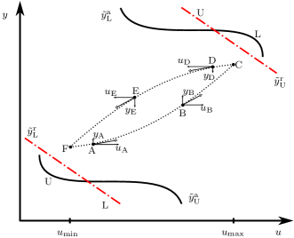
Figure 1: Schematic representation of hysteresis loop in the $u\times y$ plane. Attracting sets are shown in black continuous lines, whereas the repelling sets are indicated in red dash-dot. The hysteresis loop is indicated by dotted lines.

As a final remark, it is important to point out that the assumption that the set $\tilde{y}$ comes in two disjoint parts, either for loading or unloading, is a consequence of the solution of (7) being rational instead of polynomial. This is useful to analyse models with more general model structures.

The following example illustrates the application of this analysis and show which constraints should be considered to comply with Property 1.

Example 1

Consider the following NARX model that complies with Assumption 1:

$$y_{k} {=}\theta_{1}y_{k-1}+\theta_{2}\phi_{2,\,k-1}{+}\theta_{3}\phi_{1,\,k-1}u_{k-1}$$ (9)

$${+}\theta_{4}\phi_{2,\,k-1}\phi_{1,\,k-1}y_{k-1}{+}\theta_{5}\phi_{1,\,k-1}.$$

In this case, the constraint $\theta_{1}=1$ will be used such that, according to Lemma 1, the resulting model will have a continuum of equilibrium points. This can be achieved using estimator (5) with $c=1$ and $S=[1\,\,0\,\,0\,\,0\,\,0]$.

For a more complicated model structure, the constraint in Lemma 1 is still in the form $1=S\bm{\theta}$ (4) but with $S$ having more that one element equal to one, e.g. as shown in [42] to obtain NARX models able to reproduce dead-zone and in [43] for a quadratic nonlinearity.

The quasi-static analysis of model (9) is performed following the steps provided in section 3.2. So rewriting this model as (7), we have

$$\tilde{y} \approx \theta_{1}\tilde{y}{+}\theta_{2}{\phi}_{2,k-1}{+}\theta_{3}{\phi}_{1,k-1}u_{k-1}$$

$$+\theta_{4}{\phi}_{2,k-1}{\phi}_{1,k-1}\tilde{y}{+}\theta_{5}{\phi}_{1,k-1},$$

which can be described by

$$\tilde{y}({u},{\phi}_{1},{\phi}_{2}){=}\cases{\frac{\theta_{2}+\theta_{3}{\phi}_{1}{u}+\theta_{5}{\phi}_{1}}{1-\theta_{1}-\theta_{4}{\phi}_{1}},{\rm for}\,\,{\phi}_{2}{=}\,\,\,1;\\ \frac{-\theta_{2}+\theta_{3}{\phi}_{1}{u}+\theta_{5}{\phi}_{1}}{1-\theta_{1}+\theta_{4}{\phi}_{1}},{\rm for}\,\,{\phi}_{2}{=}-1,\\ }$$ (10)

where the time indices have been omitted for simplicity. Therefore, the solution given at the top in (10) represents the set $\tilde{y}_{\rm L}$, while the bottom is the set $\tilde{y}_{\rm U}$.

To define whether the solutions to (10) are in the attracting or repelling regions, (8) should be computed for model (9) as

$$-1< \theta_{1}+\theta_{4}{\phi}_{2,k-1}{\phi}_{1,k-1} <1,$$

$$\frac{-1-\theta_{1}}{\theta_{4}\phi_{2,k-1}}< {\phi}_{1,k-1} <\frac{1-\theta_{1}}{\theta_{4}\phi_{2,k-1}}.$$ (11)

Since it is assumed that the known input $u_{k}$ is a non-zero loading-unloading signal, then the conditions (1) to ensure that the solutions (10) are in attracting regions can be readily verified numerically. In sections 5 and 6, the same analyses will be performed for the identified models. $\square$

4 Compensator Design

The proposed strategies to design compensators based on NARX models are detailed in this section, starting with some preliminary assumptions. In this paper, a key point is to investigate if hysteresis in the models  estimated according to section 3 have any impact on the regulation performance.

4.1 Preliminaries

Given a nonlinear system $\mathcal{S}$, the first step is to obtain hysteretic models for $\mathcal{S}$; see figure 2(a). To achieve that, two procedures will be followed. The first one aims at identifying a model $\mathcal{M}$ based on the direct relationship between $u$ and $y$, whose simulation yields $\hat{y}_{k}$, according to section 4.2. The second procedure is based on the identification of the inverse relationship, in which case a model $\breve{\mathcal{M}}$ is obtained to yield $\hat{u}_{k}$, as illustrated in figure 2(a) and following section 4.3. In the second step, the identified model is used to design a compensator $\mathcal{C}$ that yields the compensation signal $m_{k}$ for a given reference $r_{k}$; see figure 2(b).

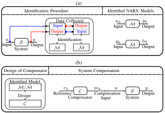
Figure 2: Compensator design based on identified NARX models. (a) Model identification, and (b) compensator design based on identified models.

In this paper,the following additional assumptions are made for NARX models (2).

Remark 1

For compensation design, $y_{k}$ can be replaced by $r_{k}$, and $u_{k}$ by $m_{k}$, respectively, in the models $\mathcal{M}$ and $\breve{\mathcal{M}}$. $\square$

The motivation behind this is that $y_{k}$ should ideally be equal to $r_{k}$ under compensation, that is, when $m_{k}$ is used as an input to the dynamical system.

In what follows, the main idea is to use an identified model to determine the compensation input $m_{k-\tau_{\rm d}+1}$.

4.2 Model-Based Compensation

The aim here is to specify a general model structure for $\mathcal{M}$ in order to find $m_{k}$ analytically from this model. To achieve that, the following assumptions are needed.

Assumption 2

Assume that: (i) the only regressor involving $u_{k-\tau_{\rm d}}$ is linear; (ii) $n_{u}>\tau_{\rm d}$; (iii) the compensation signal $m_{k}$ is known up to time $k-\tau_{\rm d}$; and (iv) the reference signal $r_{k}$ is known up to time $k+1$. $\square$

Assumption 2 imposes conditions on the selection of the model structure. Note that (i) ensures that $u_{k-\tau_{\rm d}}$ can be isolated in the identified models; (ii) allows that input terms with a delay longer than $\tau_{\rm d}$ to be regressors in the identification procedure; and the other constraints guarantee that the control action can be computed from known values. Therefore, the model $\mathcal{M}$ is rewritten as

$$A(q)y_{k}{=}B(q)u_{k}{+}f\big{(}y_{k-1},{\cdots},y_{k-n_{y}},u_{k-\tau_{\rm d}-1},{\cdots},u_{k-n_{u}}\big{)}\!,$$ (12)

where $q^{-1}$ is the backward time-shift operator such that $q^{-1}u_{k}{=}u_{k-1}$, and the linear regressors are grouped in $A(q)y_{k}$ and $B(q)u_{k}$ with

$$A(q) = 1-a_{1}q^{-1}-a_{2}q^{-2}-\cdots-a_{n_{y}}q^{-n_{y}},$$ (13)

$$B(q) = b_{\tau_{\rm d}}q^{-\tau_{\rm d}}+\underbrace{b_{\tau_{\rm d}+1}q^{-\tau_{\rm d}-1}+\cdots+b_{n_{u}}q^{-n_{u}}}_{B^{*}(q)},$$ (14)

and $f(\cdot)$ includes all the nonlinear terms and possibly the constant term of the NARX model (2). Using (14), model (12) can be rewritten as

$$A(q)y_{k} = b_{\tau_{\rm d}}u_{k-\tau_{\rm d}}{+}B^{*}(q)u_{k}{+}f\big{(}y_{k-1},\cdots,y_{k-n_{y}},$$ (15)

$$\hskip 56.9055ptu_{k-\tau_{\rm d}-1},\cdots,u_{k-n_{u}}\big{)}.$$

From Remark 1, we have

$$A(q)r_{k{+}1} = b_{\tau_{\rm d}}m_{k-\tau_{\rm d}+1}{+}B^{*}(q)m_{k{+}1}{+}f\big{(}r_{k},\cdots,$$ (16)

$$\hskip 14.22636ptr_{k-n_{y}{+}1},m_{k-\tau_{\rm d}},\cdots,m_{k-n_{u}{+}1}\big{)},$$

which, for convenience, has been written an instant of time ahead, i.e. $k\rightarrow k+1$.

From the Assumption 2, the compensation input can be obtained from (16) as

$$m_{k-\tau_{\rm d}+1} = \frac{1}{b_{\tau_{\rm d}}}\Big{[}A(q)r_{k{+}1}-B^{*}(q)m_{k{+}1}-f\big{(}r_{k},\cdots,$$ (17)

$$\hskip 14.22636ptr_{k-n_{y}{+}1},m_{k-\tau_{\rm d}},\cdots,m_{k-n_{u}{+}1}\big{)}\Big{]}.$$

To illustrate the application of this strategy, assume that the constraints discussed in section 3 and Assumption 2 are verified in the identification procedure.

Example 2

Consider the NARX model described by

$$y_{k} {=}\theta_{1}y_{k-1}{+}\theta_{2}{\phi}_{2,\,k-2}{+}\theta_{3}{\phi}_{1,\,k-2}u_{k-2}$$ (18)

$${+}\theta_{4}{\phi}_{2,\,k-2}{\phi}_{1,\,k-2}y_{k-1}{+}\theta_{5}{\phi}_{1,\,k-1}.$$

Since $\phi_{1,\,k}{=}u_{k}-u_{k-1}$ and $\phi_{2,\,k}{=}{\rm sign}(\phi_{1,\,k})$, we have

$$y_{k} {=}\theta_{1}y_{k-1}{+}\theta_{2}{\rm sign}(u_{k-2}-u_{k-3}){+}\theta_{3}[u_{k-2}-u_{k-3}]u_{k-2}$$

$${+}\theta_{4}{\rm sign}(u_{k-2}{-}u_{k-3})[u_{k-2}{-}u_{k-3}]y_{k-1}{+}\theta_{5}[u_{k-1}{-}u_{k-2}],$$

which is in the form (12) and, therefore,

$$A(q)y_{k}{=}B(q)u_{k}{+}f\big{(}y_{k-1},u_{k-2},u_{k-3},{\rm sign}(u_{k-2}-u_{k-3})\big{)},$$ (19)

where

$$A(q) = 1-\theta_{1}q^{-1},$$ (20)

$$B(q) = \theta_{5}q^{-1}-\theta_{5}q^{-2},$$ (21)

$$f(\cdot) = \theta_{2}{\rm sign}(u_{k-2}-u_{k-3}){+}\theta_{3}[u_{k-2}-u_{k-3}]u_{k-2}$$ (22)

$${+}\theta_{4}{\rm sign}(u_{k-2}-u_{k-3})[u_{k-2}-u_{k-3}]y_{k-1}.$$

From Remark 1, the model (19) is recast as

$$A(q)r_{k{+}1}{=}\theta_{5}m_{k}{-} \theta_{5}m_{k-1}{+}f\big{(}r_{k},m_{k-1},m_{k-2},$$ (23)

$${\rm sign}(m_{k-1}-m_{k-2})\big{)},$$

and

$$m_{k} = \frac{1}{\theta_{5}}\Big{[}A(q)r_{k{+}1}{+}\theta_{5}m_{k-1}$$ (24)

$$\hskip 5.69046pt-f\big{(}r_{k},m_{k-1},m_{k-2},{\rm sign}(m_{k-1}{-}m_{k-2})\big{)}\Big{]},$$

$$= \frac{1}{\theta_{5}}\Big{[}r_{k{+}1}-\theta_{1}r_{k}{+}\theta_{5}m_{k-1}$$

$$\hskip 5.69046pt-\theta_{2}{\rm sign}(m_{k-1}{-}m_{k-2})-\theta_{3}[m_{k-1}{-}m_{k-2}]m_{k-1}$$

$$\hskip 5.69046pt-\theta_{4}{\rm sign}(m_{k-1}{-}m_{k-2})[m_{k-1}{-}m_{k-2}]r_{k}\Big{]},$$

which is computed due to Assumption 2. $\square$

4.3 Compensation Based on Compensator Identification

Here, the strategy is to identify NARX models $\breve{\mathcal{M}}$ that are able to describe the inverse relationship between the input $u$ and output $y$ signals of the system $\mathcal{S}$. The advantage of this strategy is that the compensator $\mathcal{C}$ is obtained directly from $\breve{\mathcal{M}}$, according to the variable solutions presented in Remark 1. However, some issues related to the identification procedure of these models need to be addressed. For nomenclature simplicity, in this section, we assume that $\tau_{\rm d}=1$.

For the inverse model $\breve{\mathcal{M}}$, the output $\hat{u}_{k}$ depends on $y_{k}$. Hence in order to avoid the lack of causality, $y_{k}$ should be delayed by $\tau_{\rm s}$ time steps with respect to $u_{k}$, yielding [44]:

$$\hat{u}_{k}{=}\breve{F}\big{(}\hat{u}_{k-1},\cdots,\hat{u}_{k-n_{u}},y_{k-1{+}\tau_{\rm s}},\cdots,y_{k-n_{y}+\tau_{\rm s}}\big{)},$$ (25)

where $\breve{F}(\cdot)$ is the inverse nonlinear function and $\hat{u}_{k}\in\mathbb{R}$ and $y_{k}\in\mathbb{R}$ are related as shown in figure 2(a). It should be noted that $\tau_{\rm s}\geq\tau_{\rm d}+1$, where usually the equality is preferred. Similar ways to avoid noncausal models can be found in the literature [45, 29].

Assumption 3

Assume that: (i) there is at least one regressor of the output $(y_{k})^{j}$ for $j\geq 1$; (ii) the compensation signal $m_{k}$ is known up to time $k-1$; and (iii) the reference signal $r_{k}$ is known up to time $k-1+\tau_{\rm s}$. $\square$

Assumption 3 should be imposed during the structure selection of the inverse model $\breve{\mathcal{M}}$. Note that (i) ensures that there is at least one input signal $y_{k}$ in the identified models; (ii) and (iii) ensure that the compensation input $m_{k}$ to be computed at time $k$ is the only unknown variable. Given Assumption 3 and Remark 1, the compensation signal $m_{k}$ can be obtained directly from $\breve{\mathcal{M}}$ as

$$m_{k}{=}\breve{F}\big{(}m_{k-1},\cdots,m_{k-n_{u}},r_{k-1{+}\tau_{\rm s}},\cdots,r_{k-n_{y}+\tau_{\rm s}}\big{)}.$$ (26)

5 Numerical Results

This section identifies models to predict the behavior of a hysteretic system from simulated data, and evaluates the performance of these models in predicting dynamics and compensating the nonlinearity of the simulated system.

5.1 Identification of a bench test system

Consider the piezoelectric actuator with hysteretic nonlinearity modeled by the Bouc-Wen model [12] and whose mathematical model is given by [45]

$$\cases{\dot{h}(t)=~{}A\dot{u}(t)-\beta|\dot{u}(t)|h(t)-\gamma\dot{u}(t)|h(t)|,\\ y(t)=~{}d_{\rm p}u(t)-h(t),\\ }$$ (27)

where $y(t)$ is the displacement, $u(t)$ is the voltage applied to the actuator, $d_{\rm p}=1.6\,{\rm\frac{\mu m}{V}}$ is the piezoelectric coefficient, $h(t)$ is the hysteretic nonlinear term and $A=0.9\,{\rm\frac{\mu m}{V}}$, $\beta=0.008\,{\rm V^{-1}}$ and $\gamma=0.008\,{\rm V^{-1}}$ are parameters that determine the shape and scale of the hysteresis loop.

Model (27) was integrated numerically using a fourth-order Runge-Kutta method with integration step $\delta t=0.001\,{\rm s}$. The excitation signal was generated by low-pass filtering a white Gaussian noise [6]. In this work, a fifth-order low-pass Butterworth filter with a cutoff frequency of $1$ Hz was used; see figure 3(a). The sampling time is set to $T_{\rm s}=\delta t=0.001\,{\rm s}$ and a frequency of $1$ Hz is chosen to validate the identified models [45]. The data sets are $50\,{\rm s}$ long $(N=50000)$.

The constraints defined in section 3 are here considered to build NARX models for system (27). Input and output signals are shown in figure 3. In addition to the monomial regressors in $u_{k}$ and $y_{k}$, the following regressors are also used: $\phi_{1,\,k}=u_{k}-u_{k-1}$ and the sign of this first difference $\phi_{2,\,k}={\rm sign}(\phi_{1,\,k})$. The maximum nonlinear degree for regressors is cubic, $\ell=3$, and the maximum delays are $n_{y}=n_{u}=1$. This choice is based on the fact that discrete models of hysteresis that have only unit delayed regressors typically perform well and result in models with simple structures, which are advantageous for model-based control [6, 29].

The model structure is selected using the ERR criterion to rank the regressors according to importance and the AIC determine the final number of model terms. In this case, the standard least squares solution is used for parameter estimation. Also, as proposed in section 3, to obtain models that describe some features of hysteresis, the constrained parameter estimation was used in order to comply with the condition established in Property 1.

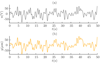
Figure 3: Signals used to identify system (27). (a) excitation, and (b) simulated output.

5.1.1 Estimating $\mathcal{M}$.

In this example we take the following metaparameters: $n_{u}=2$ which is the smallest value that complies with Assumption 2-(ii); while $n_{y}$ and $\ell$ maintain the values which were determined above. Using the data shown in figure 3 and considering Assumption 1, the following model structure is obtained

$$y_{k} =\theta_{1}y_{k-1}+\theta_{2}\phi_{1,\,k-1}+\theta_{3}\phi_{2,\,k-2}\phi_{1,\,k-2}u_{k-2}$$ (28)

$$+\theta_{4}\phi_{2,\,k-2}\phi_{1,\,k-2}y_{k-1}+\theta_{5}\phi_{1,\,k-2}u^{2}_{k-2}$$

$$+\theta_{6}\phi_{1,\,k-2}u_{k-2}y_{k-1},$$

where $\theta_{i}$ for $i=1,\cdots,6$ are estimated by least squares.

In steady-state, we have $y_{k}=\bar{y},\,\forall k$, $\phi_{1,\,k}=0,\,\forall k$; hence, the resulting expression is $\bar{y}=\theta_{1}\bar{y}$. Therefore, based on Lemma 1 and Example 1, for model (28) to fulfill Property 1, the constraint $\Sigma_{y}=\theta_{1}=1$ should be imposed. This can be done using (5) with the constraint written as:

$$c=1;\qquad S{=}[1~{}~{}0~{}~{}0~{}~{}0~{}~{}0~{}~{}0].$$ (29)

Hence, the parameter values estimated by the constrained least squares estimator (5) are shown in Table 1.

Table 1: Model parameters obtained with (5) and (29).

Model	Values
(28)	$\theta_{1}{=}1.00$	$\theta_{2}{=}0.77$
	$\theta_{3}{=}1.44\times 10^{-2}$	$\theta_{4}{=}-9.60\times 10^{-3}$
	$\theta_{5}{=}3.15\times 10^{-4}$	$\theta_{6}{=}-2.47\times 10^{-4}$
(33)	$\theta_{1}{=}1.00$	$\theta_{2}{=}1.27$
	$\theta_{3}{=}-2.13\times 10^{-2}$	$\theta_{4}{=}1.37\times 10^{-2}$
	$\theta_{5}{=}-1.07\times 10^{-5}$	$\theta_{6}{=}7.99\times 10^{-6}$

Next, a quasi-static analysis of the identified model is performed as discussed in section 3.2 and illustrated in Example 1. First, we write for (28) the corresponding to (7) as

$$\tilde{y} \approx \theta_{1}\tilde{y}+\theta_{2}{\phi}_{1,k-1}+\theta_{3}{\phi}_{2,k-2}{\phi}_{1,k-2}u_{k-2}$$

$${+}\theta_{4}{\phi}_{2,k-2}{\phi}_{1,k-2}\tilde{y}\!+\!\theta_{5}{\phi}_{1,k-2}u_{k-2}^{2}\!+\!\theta_{6}{\phi}_{1,k-2}u_{k-2}\tilde{y},$$

yielding

$$\tilde{y}({u},{\phi}_{1},{\phi}_{2}){=}\cases{\frac{\theta_{2}{\phi}_{1}+\theta_{3}{\phi}_{1}{u}+\theta_{5}{\phi}_{1}{u}^{2}}{1-\theta_{1}-\theta_{4}{\phi}_{1}-\theta_{6}{\phi}_{1}{u}},{\rm for}\,\,{\phi}_{2}{=}\,\,\,1;\\ \frac{\theta_{2}{\phi}_{1}-\theta_{3}{\phi}_{1}{u}+\theta_{5}{\phi}_{1}{u}^{2}}{1-\theta_{1}+\theta_{4}{\phi}_{1}-\theta_{6}{\phi}_{1}{u}},{\rm for}\,\,{\phi}_{2}{=}-1,}$$ (30)

where the time indices have been omitted for brevity.

The top expression in (30) gives the set $\tilde{y}_{\rm L}$, while the bottom one, $\tilde{y}_{\rm U}$. Computing the derivative of (28) with respect to $y_{k-1}$ and using (8), we obtain

$$-1<\quad\theta_{1}+\theta_{4}\phi_{1,k-2}{\phi}_{2,k-2}+\theta_{6}{\phi}_{1,k-2}u_{k-2}\quad<1,$$

$$\frac{-1-\theta_{1}-\theta_{4}\phi_{1,k-2}{\phi}_{2,k-2}}{\theta_{6}\phi_{1,k-2}}<u_{k-2}<\frac{1-\theta_{1}-\theta_{4}\phi_{1,k-2}{\phi}_{2,k-2}}{\theta_{6}\phi_{1,k-2}}.$$ (31)

Taking ${\phi}_{2,k-2}{=}1$ or ${\phi}_{2,k-2}{=}-1$, the conditions for attracting regions under load or unloading, respectively, are obtained. Considering the parameter values presented in Table 1 and a loading-unloading input signal, the points (30) and their attraction conditions (5.1.1) are computed numerically and shown in figure 4. Figure 4 should be compared to figure 1, whose main elements are analogous. Hence, in this way it is possible to see how model (28) is able to describe the hysteresis nonlinearity.

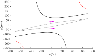
Figure 4: Results of quasi-static analysis for model (28) with input $u_{k}{=}70\sin(2\pi k)\,{\rm V}$. The hysteresis loop indicated with ($\cdots$) is a result of the interaction of (—) attracting ($\tilde{y}_{\rm L}^{\rm a}$, $\tilde{y}_{\rm U}^{\rm a}$) and (-$\,\cdot\,$-) repelling ($\tilde{y}_{\rm L}^{\rm r}$, $\tilde{y}_{\rm U}^{\rm r}$) sets. () indicates the orientation of the hysteresis loop.

Model (28) is simulated with a loading-unloading input (see left side of figure 5) and, in cases where the input becomes constant, either during loading or unloading (see right side of figure 5), the system remains at the corresponding point of the hysteresis loop. This is a direct consequence of using Lemma 1. This feature is not generally present in identified models found in the literature.

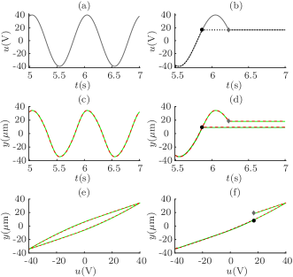
Figure 5: Free-run simulation of model (28). This figure is arranged in columns, which have: (a) sinusoidal input of voltage $u_{k}{=}40\sin(2\pi k)\,{\rm V}$ and in (b) the case where this input becomes constant during a loading ($\bullet$) and unloading ($\blacklozenge$) regime with the final value of $16.8\,{\rm V}$, its temporal responses are shown in (c) and (d) while the hysteresis loops are in (e) and (f), respectively. (—) represents the measured data and (- -) is the estimated output of the model. The full records have $N=50000$ data points.

The mean absolute percentage error (MAPE)

$${\rm MAPE}=\frac{100\sum_{k=1}^{N}|y_{k}-\hat{y}_{k}|}{N|\max(\bm{y})-\min(\bm{y})|},$$ (32)

computed for the case in figure 5(c), is shown in Table 2.

5.1.2 Estimating $\breve{\mathcal{M}}$.

The identified model that complies with Assumptions 1 and 3 is given by

$$\hat{u}_{k} =\theta_{1}\hat{u}_{k-1}+\theta_{2}\breve{\phi}_{1,\,k-1}+\theta_{3}\breve{\phi}_{2,\,k-1}\breve{\phi}_{1,\,k-1}\hat{u}_{k-1}$$ (33)

$$+\theta_{4}\breve{\phi}_{2,\,k-1}\breve{\phi}_{1,\,k-1}y_{k-1}+\theta_{5}\breve{\phi}_{2,\,k-1}y_{k-1}\hat{u}_{k-1}$$

$$+\theta_{6}\breve{\phi}_{2,\,k-1}y^{2}_{k-1},$$

where $\breve{\phi}_{1,\,k}=y_{k}-y_{k-1}$, $\breve{\phi}_{2,\,k}={\rm sign}(\breve{\phi}_{1,\,k})$, $\hat{u}_{k}$ is the estimated input (model output), and $y_{k}$ is the output of system (27) (model input).

Note that the regressors of (28) and of (33) are different. In both cases, the regressors are automatically chosen from the pool of candidates using the ERR criterion. Nevertheless, also for (33), the steady-state analysis yields $\bar{\hat{u}}{=}\theta_{1}\bar{\hat{u}}$, which is similar to the result found for model (28). Proceeding as before, the constrained least squares estimated parameters are shown in Table 1.

Consider now the quasi-static analysis of model (33). The formation of the hysteresis loop for this model is shown in figure 6. Interestingly, the ability of model (28) to describe hysteresis is also present in model (33). The main difference between them is the orientation of the hysteresis loop, as discussed in [46] and illustrated in figures 4 and 6.

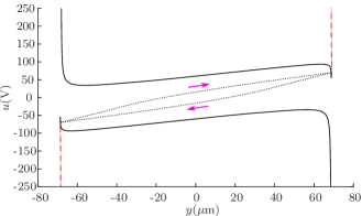
Figure 6: Results of quasi-static analysis for model (33). For meaning of line patterns refer to captions of figure 1 and of figure 4.

Table 2 shows the prediction performance of models (28) and (33) are similar. In addition, Table 2 reports the prediction performance of a black-box NARX polynomial model. The results obtained for (33) are similar to those shown in figure 5 and are omitted for brevity.

Table 2: Performance of the modeling step. Simulation results.

Design Strategy	Model	MAPE
Section 4.2	(28)	$0.398$
Section 4.3	(33)	$0.413$
Black-box	not shown	$1.494$

5.2 Compensation of a bench test system

Next, the models identified in the previous section are used to design compensators using the procedure illustrated in figure 2(b).

5.2.1 Design of the compensation input signals.

Applying the steps described in section 4.2 to model (28), the following compensation signal is obtained

$$m_{k}{=}\frac{1}{\theta_{2}} \Big{[}r_{k{+}1}-\theta_{1}r_{k}{+}\theta_{2}m_{k-1}$$ (34)

$${-}[\theta_{3}m_{k-1}{+}\theta_{4}r_{k}]{\rm sign}(m_{k-1}{-}m_{k-2})[m_{k-1}{-}m_{k-2}]$$

$${-}[\theta_{5}m^{2}_{k-1}{+}\theta_{6}m_{k-1}r_{k}][m_{k-1}-m_{k-2}]\Big{]}.$$

Similarly, using the method described in section 4.3 to identify the inverse model (33), the following compensation signal is obtained

$$\breve{m}_{k} =\theta_{1}\breve{m}_{k-1}{+}\theta_{2}[r_{k{+}1}-r_{k}]$$ (35)

$$+[\theta_{3}\breve{m}_{k-1}+\theta_{4}r_{k{+}1}]{\rm sign}(r_{k{+}1}-r_{k})[r_{k{+}1}-r_{k}]$$

$$+[\theta_{5}r_{k{+}1}\breve{m}_{k-1}+\theta_{6}r^{2}_{k{+}1}]{\rm sign}(r_{k{+}1}-r_{k}).$$

Since the parameters of compensators (34) and (35) have been estimated (Table 1), and Assumptions 2 and 3 are satisfied, the compensation inputs $m_{k}$ and $\breve{m}_{k}$ can be computed.

5.2.2 Evaluating the performance of the compensation.

The results are summarized in figure 7(b). From the hysteresis loops shown in figure 7(c), it is clear that the compensators enforced a practically linear relation between the reference and the output. This would greatly facilitate the design and increase the performance of a feedback controller.

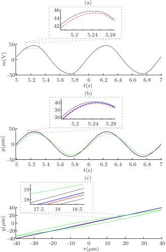
Figure 7: Hysteresis compensation for the piezoelectric actuator (27). (a) Compensation inputs, (b) temporal responses and in (c) hysteresis loops. (- -) results obtained with compensator (34) ($\cdots$) results with compensator (35), (-$\,\cdot\,$-) system output without compensation, and (—) displacement reference $r=40\sin(2\pi t)\,\mu$m.

The accuracy achieved by each compensator was quantified by the MAPE index (32). In order to quantify the compensation effort, the normalized sum of the absolute variation of the input (NSAVI)

$${\rm NSAVI}=\sum_{k=1}^{N-1}\frac{\big{|}m_{k+1}-m_{k}\big{|}}{\big{|}r_{k+1}-r_{k}\big{|}},$$ (36)

is calculated. These indices are shown in Table 3.

Table 3: Performance of the compensation step. Simulation results.

Design Strategy	Compensator	MAPE	NSAVI
Section 4.2	(34)	$0.322$	$1.13$
Section 4.3	(35)	$0.425$	$1.14$
Black-box	not shown	$1.819$	$1.15$
no compensation		$6.536$	$1.00$

The results shown in figure 7 and Table 3 indicate that the compensators may provide a significant improvement in the tracking performance of system (27). The tracking error was reduced by about $93\%$ at the cost of a $14\%$ increase in the compensation effort. Although the compensator strategies yield similar results, the design strategy of section 4.2 yielded results with lower compensation effort and tracking error.

To further characterize the performance of the proposed designs, the influence of the sampling time $T_{\rm s}$ is also investigated. In figure 8, it can be seen that the model accuracy somewhat deteriorates as $T_{\rm s}$ is increased. It should be noted that even the largest values of $T_{\rm s}$ in figure 8 are still comfortably small in terms of the sampling theorem. However, since one of the regressors is the first difference of the input, then the identification of systems with hysteresis seems to be particularly sensitive to the sampling time [47]. Another conclusion that can be drawn from figure 8 is that, for both design strategies, the compensation performance is correlated to the model accuracy, and that the strategy in section 4.2 (figure 8(a)) is somewhat less sensitive to such accuracy.

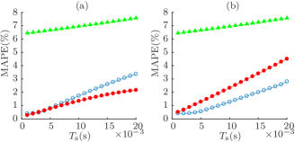
Figure 8: MAPE index (32) computed for the models and compensators described, respectively, by equations (a) (28) and (34); (b) (33) and (35). ($\circ$) model and ($\bullet$) tracking accuracies. ($\blacktriangle$) accuracy of uncompensated system.

Finally, the same analysis was carried out for situations with different shapes of the hysteresis loop varying $\beta$ in the range $0.004\leq\beta\leq 0.1$ with increments of $\Delta=0.002$ (see figure 9). The results are quite similar to the ones described so far and are not shown.

Figure 9: Bouc-Wen hysteresis loops within the investigated range.

6 Experimental Results

Both identification and compensation strategies are now applied to an experimental pneumatic control valve. This type of actuator is widely used in industrial processes, for which control performance can degrade significantly due to valve problems caused by nonlinearities [48] such as friction [49, 50], dead-zone, dead-band and hysteresis [2]. Hence, in this section we aim at compensation hysteresis using the developed techniques.

The measured output is the stem position of the pneumatic valve and the input is a signal that, after passing V/I and I/P conversion, becomes a pressure signal applied to the valve. The sampling time is $T_{\rm s}=0.01\,{\rm s}$. For model identification, the input is set as white noise low-pass filtered at $0.1\,{\rm Hz}$. For model validation, the input is a sinusoid with frequency $0.1\,{\rm Hz}$. Both data sets are $200\,{\rm s}$ long ($N=20000$). The identification of the direct $\mathcal{M}$ and inverse $\breve{\mathcal{M}}$ models was performed as in section 5. The pool of candidate terms is generated with $\ell=3$, $n_{y}=1$ and $n_{u}=2$. The model parameters are estimated using (5) in order to comply with Lemma 1.

The estimated model $\mathcal{M}$ is

$$y_{k} =y_{k-1}-19.76\phi_{1,\,k-2}+19.32\phi_{1,\,k-1}$$ (37)

$${+}9.44\phi_{2,\,k{-}2}\phi_{1,\,k{-}2}u_{k{-}2}{-}12.61\phi_{2,\,k{-}2}\phi_{1,\,k{-}2}y_{k{-}1},$$

and the inverse model $\breve{\mathcal{M}}$ is

$$\hat{u}_{k} =\hat{u}_{k{-}1}+86.67\breve{\phi}_{1,\,k{-}1}-85.02\breve{\phi}_{1,\,k{-}2}{-}0.98\breve{\phi}_{1,\,k{-}1}y_{k{-}2}$$ (38)

$$+1.72\breve{\phi}_{2,\,k{-}2}\breve{\phi}_{1,\,k{-}2}y_{k{-}2}{-}1.13\breve{\phi}_{2,\,k{-}2}\breve{\phi}_{1,\,k{-}2}\hat{u}_{k{-}1},$$

which was estimated from a smoothed version of $y_{k}$ obtained by quadratic regression. This is done only to estimate $\breve{\mathcal{M}}$ to avoid the error-in-the-variables problem, since $y_{k}$ serves as the input for $\breve{\mathcal{M}}$. Each model performance is given in figure 10 and Table 4.

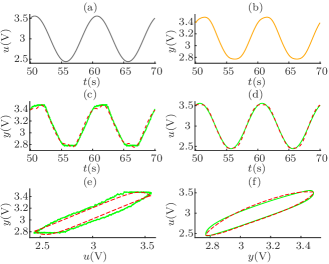
Figure 10: Left column refers to model (37) and right column to model (38). (a) input $u_{k}{=}0.56\sin(0.2\pi k)+3\,{\rm V}$ and (c) the corresponding measured output (—) $y$ and (- -) model (37) free-run simulation; (b) smoothed version of $y$ in (c); (d) the corresponding output which is $u_{k}$ in (a) and (- -) model (38) free-run simulation. (e) and (f) show the same data as (c) and (d), respectively.

Table 4: Performance of the modeling step. Experimental results.

Design Strategy	Model	MAPE
Section 4.2	(37)	$3.926$
Section 4.3	(38)	$2.374$

Models (37) and (38) are used to implement the strategies described in sections 4.2 and 4.3, thus yielding, respectively, the compensation inputs

$$m_{k}{=}\frac{1}{19.32} \!\Big{[}r_{k{+}1}{-}r_{k}{+}19.32m_{k{-}1}{+}19.76[m_{k{-}1}{-}m_{k{-}2}]$$ (39)

$$-9.44{\rm sign}(m_{k-1}-m_{k{-}2})[m_{k{-}1}-m_{k{-}2}]m_{k{-}1}$$

$${+}12.61{\rm sign}(m_{k{-}1}{-}m_{k{-}2})[m_{k{-}1}{-}m_{k{-}2}]r_{k}\Big{]}\!,$$

and

$$\breve{m}_{k} =\breve{m}_{k{-}1}{+}86.67[r_{k{+}1}-r_{k}]{-}85.02[r_{k}-r_{k{-}1}]$$ (40)

$$-0.98[r_{k{+}1}-r_{k}]r_{k}+1.72{\rm sign}(r_{k}-r_{k{-}1})[r_{k}-r_{k{-}1}]r_{k}$$

$$-1.13{\rm sign}(r_{k}-r_{k{-}1})[r_{k}-r_{k{-}1}]\breve{m}_{k-1}.$$

The results of the experiment are shown in figure 11 and assessed in Table 5. Note that both approaches significantly reduce the tracking error. Based on both numerical and experimental results, it seems that the performance of the compensators is directly related to the accuracy of the identified model; see Table 4 and Table 5. Hence, as before, these results suggest that the compensation effort tends to be lower and more effective whenever the identified models are more accurate.

The compensation produced by (40) is smoother than the one obtained with (39); see figure 11(a). This occurs because, for the compensator (40), the argument of the sign function depends on the difference of the reference signal, while, for the compensator (39), it depends on the difference of the autoregressive variable which usually produces stronger oscillations and sudden changes; see figure 11(a), e.g. in the range of $51{-}53\,{\rm s}$. As a result, larger compensation effort is required as quantified by NSAVI (36) in Table 5.

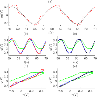
Figure 11: Hysteresis compensation for the pneumatic valve. (a) Compensation inputs, (b) and (c) its temporal responses and in (d) and (e)  the hysteresis loops. (- -) illustrates the results obtained with compensator (39), ($\cdots$) refers to the results by using compensator (40), (-$\,\cdot\,$-) the system output without compensation, and (—) the reference $r{=}0.56\sin(0.2\pi t){+}3\,{\rm V}$.

Table 5: Performance of the compensation step. Experimental results.

Design Strategy	Compensator	MAPE	NSAVI
Section 4.2	(39)	$5.514$	$1.81$
Section 4.3	(40)	$2.939$	$1.61$
no compensation		$18.602$	$1.00$

7 Conclusions

This work addressed the problems of identification and compensation of hysteretic systems. In the context of system identification, the contribution is twofold. First, we build models with regressors that use the sign function of the first difference of the input, as proposed by [6], and present an additional condition in order to guarantee a continuum of equilibrium points at steady-state, which is an important ingredient for hysteresis [30, 5]. To this aim, a particular constraint on the parameters is presented in Lemma 1. As a consequence, the identified models are able to describe both dynamical and static features of the hysteresis nonlinearity. Second, following a quasi-static analysis of these models, a schematic framework is proposed to explain how the hysteresis loop occurs on the input-output plane (see Figure 1).

In the context of hysteresis compensation, this paper introduces two strategies to design compensators. An important aspect of such procedures is that they show how to restrict the pool of candidate regressors aiming at solving the compensation problem. Such strategies are not limited to hysteresis and can be extended to other nonlinearities.

The effectiveness of the compensation schemes is illustrated by means of numerical and experimental tests. For the strategy described in Section 4.2, the compensation law is obtained from the identified model by simple algebraic manipulations. In the case of the strategy introduced in Section 4.3, the compensators are identified directly from the data. This, however, leads to models that are noncausal by nature. Guidelines to circumvent this problem are provided. The compensators designed by both strategies can be readily employed in online compensation schemes.

As a general remark, we observed in all our examples that the quality of the achieved compensation is correlated with the accuracy of the identified model (compare Table 2 with Table 3 and Table 4 with Table 5). Finally, we noticed that the identified models have a discontinuity due to the sign function used in some regressors. When the model has many such terms, it sometimes happens that the compensation signal presents abrupt transitions. The use of smoother functions in place of the sign function, in order to alleviate this problem, will be investigated in the future.

References

References

- [1] A Visintin. Differential Models of Hysteresis. Springer, Berlin Heidelberg, 1994.
- [2] M A A S Choudhury, S L Shah, and N F Thornhill. Diagnosis of Process Nonlinearities and Valve Stiction: Data Driven Approaches. Springer, Berlin Heidelberg, 2008.
- [3] M Rakotondrabe. Smart Materials-Based Actuators at the Micro/Nano-Scale: Characterization, Control and Applications. Springer, New York, 2013.
- [4] J Peng and X Chen. A Survey of Modeling and Control of Piezoelectric Actuators. Modern Mechanical Engineering, 3(1):1–20, 2013.
- [5] K A Morris. What is Hysteresis? Applied Mechanics Reviews, 64(5):050801, 2011.
- [6] S A M Martins and L A Aguirre. Sufficient Conditions for Rate-Independent Hysteresis in Autoregressive Identified Models. Mechanical Systems and Signal Processing, 75:607–617, 2016.
- [7] G Tao and P V Kokotovic. Adaptive Control of Plants with Unknown Hystereses. IEEE Transactions on Automatic Control, 40(2):200–212, 1995.
- [8] C Visone. Hysteresis Modelling and Compensation for Smart Sensors and Actuators. Journal of Physics: Conference Series, 138(1):012028, 2008.
- [9] H Chaoui and H Gualous. Adaptive Control of Piezoelectric Actuators with Hysteresis and Disturbance Compensation. Journal of Control, Automation and Electrical Systems, 27(6):579–586, 2016.
- [10] S Yi, B Yang, and G Meng. Ill-conditioned dynamic hysteresis compensation for a low-frequency magnetostrictive vibration shaker. Nonlinear Dynamics, 96(1):535–551, 2019.
- [11] V Hassani, T Tjahjowidodo, and T N Do. A survey on hysteresis modeling, identification and control. Mechanical Systems and Signal Processing, 49(1-2):209–233, 2014.
- [12] Y K Wen. Method for Random Vibration of Hysteretic Systems. Journal of the Engineering Mechanics Division, 102(2):249–263, 1976.
- [13] J Oh and D S Bernstein. Semilinear Duhem model for rate-independent and rate-dependent hysteresis. IEEE Transactions on Automatic Control, 50(5):631–645, 2005.
- [14] P Ge and M Jouaneh. Tracking Control of a Piezoceramic Actuator. IEEE Transactions on Control Systems Technology, 4(3):209–216, 1996.
- [15] M Brokate and J Sprekels. Hysteresis and Phase Transitions. Springer-Verlag, New York, 1996.
- [16] A W Smyth, S F Masri, E B Kosmatopoulos, A G Chassiakos, and T K Caughey. Development of Adaptive Modeling Techniques for Non-linear Hysteretic Systems. International Journal of Non-Linear Mechanics, 37(8):1435–1451, 2002.
- [17] G Quaranta, W Lacarbonara, and S F Masri. A review on computational intelligence for identification of nonlinear dynamical systems. Nonlinear Dynamics, 2020.
- [18] R W K Chan, J K K Yuen, E W M Lee, and M Arashpour. Application of Nonlinear-Autoregressive-Exogenous model to predict the hysteretic behaviour of passive control systems. Engineering Structures, 85:1–10, 2015.
- [19] H V H Ayala, D Habineza, M Rakotondrabe, C E Klein, and L S Coelho. Nonlinear black-box system identification through neural networks of a hysteretic piezoelectric robotic micromanipulator. IFAC-PapersOnLine, 48(28):409–414, 2015.
- [20] J Fu, G Liao, M Yu, P Li, and J Lai. NARX neural network modeling and robustness analysis of magnetorheological elastomer isolator. Smart Materials and Structures, 25(12):125019, 2016.
- [21] L A Aguirre. A Bird‘s Eye View of Nonlinear System Identification. arXiv:1907.06803 [eess.SY], 2019.
- [22] I J Leontaritis and S A Billings. Input-Output Parametric Models for Non-Linear Systems Part I: Deterministic Non-Linear Systems. International Journal of Control, 41(2):303–328, 1985.
- [23] I J Leontaritis and S A Billings. Input-Output Parametric Models for Non-Linear Systems Part II: Stochastic Non-Linear Systems. International Journal of Control, 41(2):329–344, 1985.
- [24] R K Pearson. Discrete-Time Dynamic Models. Oxford University Press, Oxford, 1999.
- [25] A Leva and L Piroddi. NARX-based Technique for the Modelling of Magneto-Rheological Damping Devices. Smart Materials and Structures, 11(1):79–88, 2002.
- [26] L Deng and Y Tan. Modeling Hysteresis in Piezoelectric Actuators Using NARMAX Models. Sensors and Actuators A: Physical, 149(1):106–112, 2009.
- [27] K Worden and R J Barthorpe. Identification of hysteretic systems using NARX models, Part I: evolutionary identification. In Topics in Model Validation and Uncertainty Quantification, volume 4, pages 49–56. Springer, 2012.
- [28] R Dong and Y Tan. Inverse Hysteresis Modeling and Nonlinear Compensation of Ionic Polymer Metal Composite Sensors. In Proceeding of the 11th World Congress on Intelligent Control and Automation, pages 2121–2125, Shenyang, China, 2014.
- [29] W R Lacerda Júnior, S A M Martins, E G Nepomuceno, and M J Lacerda. Control of Hysteretic Systems Through an Analytical Inverse Compensation based on a NARX model. IEEE Access, pages 1–1, 2019.
- [30] D S Bernstein. Ivory Ghost [Ask The Experts]. IEEE Control Systems Magazine, 27(5):16–17, 2007.
- [31] S A Billings and S Chen. Extended Model Set, Global Data and Threshold Model Identification of Severely Non-Linear Systems. International Journal of Control, 50(5):1897–1923, 1989.
- [32] N R Draper and H Smith. Applied regression analysis. John Wiley & Sons, New York, 3 edition, 1998.
- [33] S Chen, S A Billings, and W Luo. Orthogonal Least Squares Methods and their Application to Non-Linear System Identification. International Journal of Control, 50(5):1873–1896, 1989.
- [34] H Akaike. A New Look at the Statistical Model Identification. IEEE Transactions on Automatic Control, 19(6):716–723, 1974.
- [35] L Piroddi. Simulation Error Minimisation Methods for NARX Model Identification. International Journal of Modelling, Identification and Control, 3(4):392–403, 2008.
- [36] S A M Martins, E G Nepomuceno, and M F S Barroso. Improved Structure Detection For Polynomial NARX Models Using a Multiobjective Error Reduction Ratio. Journal of Control, Automation and Electrical Systems, 24(6):764–772, 2013.
- [37] A Falsone, L Piroddi, and M Prandini. A randomized algorithm for nonlinear model structure selection. Automatica, 60:227–238, 2015.
- [38] P F L Retes and L A Aguirre. NARMAX Model Identification Using a Randomised Approach. International Journal of Modelling, Identification and Control, 31(3):205–216, 2019.
- [39] I B Q Araújo, J P F Guimarães, A I R Fontes, L L S Linhares, A M Martins, and F M U Araújo. NARX Model Identification Using Correntropy Criterion in the Presence of Non-Gaussian Noise. Journal of Control, Automation and Electrical Systems, 30(4):453–464, 2019.
- [40] F Ikhouane and J Rodellar. Systems with Hysteresis: Analysis, Identification and Control Using the Bouc-Wen Model. John Wiley & Sons, 2007.
- [41] L A Aguirre and E M A M Mendes. Global Nonlinear Polynomial Models: Structure, Term Clusters and Fixed Points. International Journal of Bifurcation and Chaos, 6(2):279–294, 1996.
- [42] L A Aguirre. Identification of smooth nonlinear dynamical systems with non-smooth steady-state features. Automatica, 50(4):1160–1166, 2014.
- [43] L A Aguirre, M F S Barroso, R R Saldanha, and E M A M Mendes. Imposing steady-state performance on identified nonlinear polynomial models by means of constrained parameter estimation. IEE Proceedings - Control Theory and Applications, 151(2):174–179, 2004.
- [44] P Q Xia. An Inverse Model of MR Damper using Optimal Neural Network and System Identification. Journal of Sound and Vibration, 266(5):1009–1023, 2003.
- [45] M Rakotondrabe. Bouc-Wen Modeling and Inverse Multiplicative Structure to Compensate Hysteresis Nonlinearity in Piezoelectric Actuators. IEEE Transactions on Automation Science and Engineering, 8(2):428–431, 2011.
- [46] G Y Gu, M J Yang, and L M Zhu. Real-Time Inverse Hysteresis Compensation of Piezoelectric Actuators with a Modified Prandtl-Ishlinskii Model. Review of Scientific Instruments, 83(6):065106, 2012.
- [47] W R Lacerda Júnior, S A M Martins, and E G Nepomuceno. Influence of Sampling Rate and Discretization Methods in the Parameter Identification of Systems with Hysteresis. Journal of Applied Nonlinear Dynamics, 6(4):509–520, 2017.
- [48] R Srinivasan and R Rengaswamy. Stiction Compensation in Process Control Loops: A Framework for Integrating Stiction Measure and Compensation. Industrial & Engineering Chemistry Research, 44(24):9164–9174, 2005.
- [49] R A Romano and C Garcia. Valve friction and nonlinear process model closed-loop identification. Journal of Process Control, 21(4):667–677, 2011.
- [50] J R Baeza and C Garcia. Friction compensation in pneumatic control valves through feedback linearization. Journal of Control, Automation and Electrical Systems, 29(3):303–317, 2018.