Trace Clustering on Very Large Event Data in Healthcare using Frequent Sequence Patterns

Abstract

Trace clustering has increasingly been applied to find homogenous process executions. However, current techniques have difficulties in finding a meaningful and insightful clustering of patients on the basis of healthcare data. The resulting clusters are often not in line with those of medical experts, nor do the clusters guarantee to help return meaningful process maps of patients’ clinical pathways. After all, a single hospital may conduct thousands of distinct activities and generate millions of events per year. In this paper, we propose a novel trace clustering approach by using sample sets of patients provided by medical experts. More specifically, we learn frequent sequence patterns on a sample set, rank each patient based on the patterns, and use an automated approach to determine the corresponding cluster. We find each cluster separately, while the frequent sequence patterns are used to discover a process map. The approach is implemented in ProM and evaluated using a large data set obtained from a university medical center. The evaluation shows F1-scores of 0.7 for grouping kidney injury, 0.9 for diabetes, and 0.64 for head/neck tumor, while the process maps show meaningful behavioral patterns of the clinical pathways of these groups, according to the domain experts.

1 Introduction

Clinical pathways are known to be enormously complex and flexible. Process mining techniques are often applied to analyze event data related to clinical pathways, in order to obtain valuable insights [1]. The resulting findings can help to improve process quality, patient outcomes and satisfaction, and optimizing resource planning, usages, and reallocation [2]. Finding coherent, relatively homogenous patient groups helps process mining techniques to obtain accurate insights [3, 7, 4].

Many existing systems have tried to classify patients and provide such a well-defined group, known as Patient classification systems (PCSs). PCSs provide a categorization of patients based on clinical data (i.e. diagnoses, procedures), demographic data (i.e. age, gender), and resource consumption data (i.e. costs, length of stay) [5]. While useful, such systems often do not align well with the patient groups as clinicians would define them. Patients who have received the same diagnosis (codes) may be treated for different purposes. For example, patients who get reconstructive breast surgery caused by breast cancer or by gender change can be assigned to the same group, while they have different characteristics and should be assigned to different groups, according to medical experts [6]. Consequently, the process models derived for such a patient group is often also inaccurate and not aligned with the pathways which clinicians would have in their mind. As a result, much manual work involving medical experts is needed to obtain meaningful patient groups.

Emerged from the process mining discipline, trace clustering techniques aim to help finding such homogenous groups of process instances (in our case the patients) [3, 7, 8, 4]. These techniques cluster the process instances based on the similarity between the sequences of executed activities. However, when applied on hospital data, these approaches face several challenges. Firstly, they have difficulties in scaling-up to handle such large data sets, which may contain hundreds of thousands of patients and millions of events per year. Secondly, they assume that the cases within a group show more homogenous behavior than the cases of different groups, whereas in healthcare, patients treated for the same purpose could have disjoint paths and vice versa. Thirdly, feature vectors (or other intermediate models) are often used to represent the cases and to compute similarity measures; the resulting clusters are often based on an average of the measures and, therefore, may not have clear criteria and may be difficult to explain. Finally, a resulting cluster of patients could still have thousands of distinct activities, which prevents any process discovery algorithm to find a reasonable process model.

In this paper, we propose a novel perspective to the trace clustering problem. We use sample sets to find one patient cluster at a time by exploiting frequent sequential pattern mining techniques, exemplified in Fig. 1.

Figure 1: An example of the partial trace clustering problem and an overview of our approach using sample sets and frequent sequence patterns.

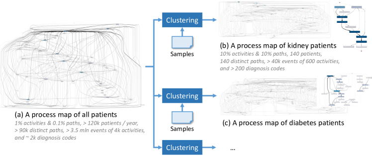
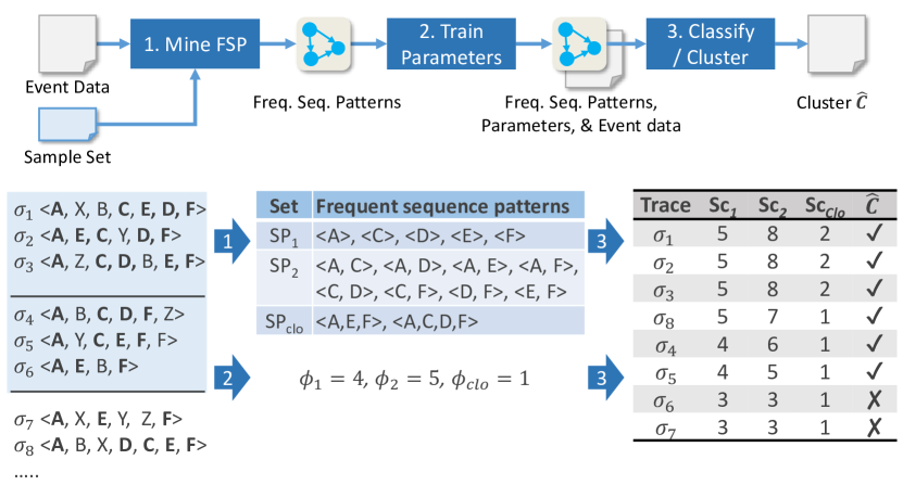
More specifically, we assume for each group a small sample set of patients (i.e., patient ids) that belongs to the group is made available by medical experts. Using the available event data of patient pathways of the sample set, we compute frequent sequence patterns (FSPs) to learn the behavioral criteria of the group. All patients are ranked based on the behavioral criteria, and we use thresholds to automatically determine whether they belong to the group (see Fig. 2, discussed in Sect. 4). Each group is clustered independently. The obtained sequence patterns are used to discover simple process maps.

The approach is implemented in the Process Mining toolkit ProM and evaluated using three real-life cases obtained from a large academic hospital in the Netherlands. The results are validated with a semi-medical expert and a data analyst of the hospital, both of them work closely with medical experts; the semi-medical expert is a manager who has acquired relevant medical knowledge regarding the patient pathways.

The contribution of this work is that it gives a concrete method to identify patient clusters from a wealth of data and high variety of pathways with relatively little input from experts. Moreover, this clustering will lead to simple process maps of frequent behavioral patterns in the clinical pathways that can be used in the communication with medical experts. Such a method may be useful to reason about clinical pathways within hospitals for the sake of process improvement or quality control.

In the remainder, we first discuss related work in Sect. 2. We recall the concepts and define the research problem in Sect. 3 The proposed approach is described in Sect. 4. The evaluation results are presented Sect. 5, and Sect. 6 concludes the paper.

2 Related Work

In this section, we discuss three streams of trace clustering techniques, categorizing them by their similarity measures.

Feature-vector-based similarity Early work in trace clustering has followed the ideas in traditional data clustering. Each trace is transformed into a vector of features based on, for example, the frequency of activities, the frequency of directly-followed relations, the resources involved, etc. Between these feature vectors, various distance metrics in data mining are reused to estimate the similarity between the traces. Subsequently, distance-based clustering algorithms are deployed, such as k-means or agglomerative hierarchical clustering algorithms [3, 7, 8].

In line with feature-vector based trace clustering techniques, the work of Greco et al. [3] was one of the first approaches that incorporated trace clustering into process discovery algorithms. Their work uses frequent (sub)sequences of activities to constitute feature vectors that represent traces. Hierarchical clusters are then built using a top-down approach which iteratively refines the most imprecise process model (represented as disjunctive workflow schemas). Song et al. [7] present a technique that generalizes the feature space by considering data attributes in other dimensions than solely focusing on the control-flow. Features of traces in one dimension are grouped into a so-called trace-profile, e.g., resource, performance, case attribute profiles, etc. Furthermore, a multitude of vector-based distance metrics and clustering techniques (both partitioning and hierarchical) are deployed. In [8], Bose and van der Aalst compute reoccurring sequences of activities, known as tandem arrays, and used these patterns as features in the feature space model in order to improve the way the control-flow information is taken into account in trace clustering.

Trace-sequence based clustering The second category proposes that the similarity can be measured by the syntax similarity between two trace sequences. A trace can be edited into another trace by adding and removing events. The similarity between two traces is measured by the number of the edit operations needed. An example of this category of measure is the Levenshtein Edit Distance (LED). Bose and van der Aalst [9] propose a trace-sequence distance by generalizing the LED and use the agglomerative clustering technique. Chatain et al. [10] assume that a normative process model is available and align the traces with the runs of the model. In essence, the traces that are close to the same run (in terms of sequence distance) are clustered into the same group.

Model-based trace clustering Recently, the aim of trace clustering to discover better models has become more prominent. Consequently, the definition of the similarity between traces has shifted from the traces themselves to the quality of the models discovered from those traces. In essence, it is proposed that a trace is more similar to a cluster of traces, if a more fitting, precise, and simple model can be discovered from the cluster [11, 12, 4].

Early work in sequence clustering used first-order Markov models as the intermediate models to represent the clusters. In 2003, Cadez et al. [11] proposed to learn a mixture of first-order Markov models from user behavior by applying the Expectation Maximization problem. The approach is evaluated on a web navigation data set. Later, Ferreira et al. [12] followed the same idea and qualitatively evaluated the clustering algorithm in a process mining setting using two additional data sets.

De Weerdt et al. [4] use Petri nets as intermediate models and optimize a F-measure of the models discovered from the clusters. The algorithm, called ActiTraC, first samples distinct traces, based on frequency or distance, as initial clusters. The traces that “fit” into the intermediate-model of a cluster are assigned to the cluster. The remaining noisy traces either are distributed over the clusters or returned as a garbage cluster. More recently, De Koninck et al. [13] proposed to incorporate domain knowledge by assuming that a complete clustering solution is provided by experts. The proposed technique then aims to improve the quality of such a complete expert-driven clustering in terms of the model qualities.

Discussion Regarding the feature-based techniques, the number of possible features can be immense, especially in process mining [7]. For example, for $n$ activities, we could have $n^{2}$ number of directly-followed relations and $n^{3}$ if we consider three activities. With thousands of distinct activities, it can be computationally expensive if we consider the full feature space. Moreover, as the clusters are calculated based on the average distances between feature vectors, it is often difficult to explain the reason of a particular clustering. In many cases, the feature-based techniques have difficulties in finding clusters that are in line with those of domain experts [13]. Sequence-based trace clustering faces similar limitations as the feature-based. Furthermore, patients who have disjoint sets of activities and diagnosis (codes) may belong to the same group. Both feature-based and sequence-based would have difficulties finding those. For model-based trace clustering techniques, it would be difficult to handle the complexity of the intermediate models. The clinical pathway of a well-defined patient group could still be extremely complex with thousands distinct activities being executed and each patient following a unique path tailored towards their conditions (see Sect. 5.1). Assuming that a complete expert-driven clustering is available would put too much effort on medical experts and is not feasible for this reason. Our approach, therefore, needs to be scalable and able to deal with this complexity. The approach should also put more emphasis on the abundant domain knowledge available and find clear behavioral criteria of the clusters such that the behavioral criteria are meaningful for domain or medical experts.

3 Research Problem

In this section, we first recall the preliminary concepts such as event logs, traces, and activities. Using these concepts, we define our research problem.

3.1 Preliminaries

A process describes a set of activities executed in a certain order. For example, each patient in a hospital follows a certain process to treat a certain diagnosis of a disease, also known as clinical pathway. An event log is a set of traces, each describing a sequence of events through the process. Each event records additional information regarding the executed activity. For example, Table 1 shows a snippet of an event log of a healthcare process. Each row records an executed event, which contains information such as the event id, the patient id, the activity, the timestamps, the diagnosis code (also known as diagnosis-related group (DRG) [5], or DBC in Dutch), and potentially some additional attributes regarding the event.

Table 1: An example of an event log of a healthcare process

Event	PID	Activity	Time stamps	DBC	Attr.
1	1001	Registration (Reg)	22-10-2018	DBC1	…
2	1001	Doctor appointment (Doc)	23-10-2018	DBC1	…
3	1001	Lab test (Lab)	24-10-2018	DBC1	…
4	1001	Surgery (Srg)	30-10-2017	DBC2	…
5	1001	Doctor appointment (Doc)	01-11-2017	DBC2	…
21	1002	Registration (Reg)	23-10-2017	DBC3	…
22	1002	Lab test (Lab)	25-10-2017	DBC3	…
23	1002	Surgery (Srg)	26-10-2017	DBC4	…
31	1003	Registration (Reg)	25-10-2017	DBC1	…
32	1003	Surgery (Srg)	26-10-2017	DBC1	…
…	…	…	…	…	…

Definition 1 (Universes)

We write the following notations for universes: $\mathcal{E}$ denotes the universe of unique events, i.e., the set of all possible event identifiers. $U$ denotes the set of all possible attribute names. $\mathit{Val}$ denotes the set of all possible attribute values. $\mathit{Act}\subset\mathit{Val}$ denotes the set of all possible activity names. $\mathit{PI}\subset\mathit{Val}$ denotes the set of all possible process instance identifiers.

Definition 2 (Event, Attribute, Label)

For each event $e\in\mathcal{E}$, for each attribute name $d\in U$, the attribute function $\pi_{d}(e)$ returns the value of attribute $d$ of event $e$. A labeling function $\pi_{l}:\mathcal{E}\rightarrow\mathit{Val}$ is a function that assigns the label to each event $e\in\mathcal{E}$.

If the value is undefined, $\pi_{d}(e)=\bot$. Examples of attribute names used in this paper are listed as follows: $\pi_{\mathit{pi}}(e)\in\mathit{PI}$ denotes the process instance identifier of $e$; $\pi_{\mathit{act}}(e)\in\mathit{Act}$ is the activity associated with $e$; $\pi_{\mathit{time}}(e)$ denotes the timestamp of $e$; $\pi_{\mathit{dbc}}(e)$ denotes the diagnosis code of $e$. For example, given the log listed in Tab. 1, $\pi_{\mathit{pi}}(e_{1})=1001$, $\pi_{\mathit{act}}(e_{1})=$ Registeration, $\pi_{\mathit{dbc}}(e_{1})=$ DBC1.

The labeling function $\pi_{l}(e)$ returns the activity label of event $e$ in the process (also known as an event classifier). In this paper, we combine both the activities and the diagnosis codes and use them as labels, i.e., $\pi_{l}(e):=\pi_{\mathit{act}}(e)+\pi_{\mathit{dbc}}(e)$, because the data analyst from the hospital indicated that both are important for the clinical pathway. For example, given the log listed in Tab. 1, the label of event 1 is $\pi_{l}(e_{1}):=\pi_{\mathit{act}}(e_{1})+\pi_{\mathit{dbc}}(e_{1})=$ “Reg-DBC1”; the label of event 23 is $\pi_{l}(e_{23})=$ “Srg-DBC4”.

A trace $\sigma=\langle e_{1},e_{2},\cdots,e_{n}\rangle\in\mathcal{E}^{*}$ is a sequence of events, where for $1\leq i<n$, $\pi_{time}(e_{i})\leq\pi_{time}(e_{i+1})$ and $\pi_{pi}(e_{i})$ = $\pi_{pi}(e_{i+1})$. An event log $L=\{\sigma_{1},\cdots,\sigma_{\mid L\mid}\}\subseteq\mathcal{E}^{*}$ is a set of traces.

Definition 3 (Simplified Trace, Simplified Log)

Let $\pi_{l}$ be the labeling function. Let $L=\{\sigma_{1},\cdots,\sigma_{\mid L\mid}\}$ be a log and $\sigma=\langle e_{1},e_{2},\cdots,e_{\mid\sigma\mid}\rangle$ a trace. We overload the labeling function such that, given $\sigma$, the labeling function returns the sequence of labels of the events in $\sigma$, i.e., $\pi_{l}(\sigma)=\langle\pi_{l}(e_{1}),\pi_{l}(e_{2}),\cdots,\pi_{l}(e_{\mid\sigma\mid})\rangle\in\mathit{Val}^{*}$. Furthermore, given the log $L$, the labeling function returns the multi-set of the sequences of the labels of the traces in $L$, i.e., $\pi_{l}(L)=[\pi_{l}(\sigma_{1}),\cdots,\pi_{l}(\sigma_{\mid L\mid})]$.

Let $\sigma=\langle e_{1},\cdots,e_{n}\rangle\in L$ be a trace. For $1\leq i<n$, we say event $e_{i}$ is directly-followed by $e_{i+1}$. For $1\leq i<j\leq n$, we say event $e_{i}$ is eventually-followed by $e_{j}$. For the sake of brevity, we write $L^{l}=\pi_{l}(L)$ and $\sigma^{l}=\pi_{l}(\sigma)$. For instance, the simplified trace of patient 1001 listed in Tab. 1 is $\pi_{l}(\sigma_{1001})=\sigma_{1001}^{act,dbc}=\langle$“Reg-DBC1”, “Doc-DBC1”, “Lab-DBC1”, “Srg-DBC2”, “Doc-DBC2”$\rangle$. Note that a patient (an activity) could be associated with multiple diagnosis codes [5], e.g., patient 1001 (activity Doc).

3.2 Research Problem - Grouping Patients

Traditional trace clustering aims to divide the traces of a log into clusters, such that the traces of the same cluster show more homogenous behavior than the traces of different clusters. In the healthcare domain, we are facing a very large, complex data set and abundant domain knowledge. As discussed at the end of Sect. 2, we would like to (1) handle such a large data set, to (2) incorporate, leverage, and put more emphasis on the domain knowledge, in order to obtain clusters that are more in line with those of medical experts, while requiring little effort from such experts, and to (3) be able to find the clusters accurately and validate clusters quality, we propose the following.

We assume that medical experts can provide a small sample set $P$ of the patients that belong to a patient group $\hat{C}$ of interest. Giving a sample requires little effort from their side. We assume that $\hat{C}$ is unknown (because when $\hat{C}$ gets large, it would require too much effort for medical experts to exhaustively list all patients that belong to $\hat{C}$ and to repeat this process). We use the available traces of all patients in the sample $P$, and the objective is to find a cluster $C$ in such a way that $C$ is as close to the group $\hat{C}$ as possible (i.e., the highest recall and precision possible). We do this separately for each group $\hat{C}_{i}$ where the sample set $P_{i}$ is available. To generalize, we define the partial trace clustering formally as follows.

Definition 4 (Partial Trace Clustering)

Let $L=\{\sigma_{1},\cdots,\sigma_{n}\}$ be the event log, and $\mathit{PI}=\{\pi_{pi}(\sigma_{1}),\cdots,\pi_{pi}(\sigma_{n})\}$ the set of case ids of $L$. Let $P_{1},P_{2},\cdots,P_{x}\subset\mathit{PI}$ be the sets of samples that respectively belong to clusters $\hat{C}_{1},\hat{C}_{2},\cdots,\hat{C}_{x}$, provided by experts (e.g., a doctor), with $x\in\mathbb{N}$. We would like to find the clusters $C_{1},C_{2},\cdots,C_{x}\subset\mathit{PI}$, such that the set difference between $C_{i}$ and $\hat{C}_{i}$ is minimized.

Note that clusters $C_{1},\cdots,C_{x}$ can be non-overlapping or form an incomplete clustering of $\mathit{PI}$ (i.e., $C_{1}\cup\cdots\cup C_{x}\subseteq\mathit{PI}$), and $x$ could be 1. Based on these properties, we do not have to find all clusters or to compute a complete clustering of all traces. It allows us to mine, cluster, and validate each cluster independently.

4 Approach

As explained above, we assume that for each cluster $C$ to be found we have a small sample $P$ of the cases that belongs to the true-but-unknown cluster $\hat{C}$. For all other cases it is unknown whether they belong to the cluster or not. By exploiting the available sample set $P$ and the event log $L$ of all cases, the objective is to find behavioral criteria for determining the cluster. To find the behavioral criteria and to handle the large number of features, we compute frequent behavioral patterns. In Sect. 4.1, we first explain the use of sequence pattern mining to learn the frequent sequence patterns (FSPs) of the sample set. In Sect. 4.2, we then match the FSPs to the other cases in the sample to train our parameters. Finally, we match all cases to the clustering criteria to return the computed cluster in Sect. 4.3. Fig. 2 shows an overview of the approach.

4.1 Finding Frequent Sequence Patterns

The first step of the approach is to find frequent sequence patterns repeated among the samples. A frequent sequence pattern is a sequence that occurs in the traces with a frequency no less than a specified threshold. We adapt the definition of sequence patterns in our context as follows.

Definition 5 (Sequence Pattern)

A sequence pattern $\vec{s}=\langle a_{1},\cdots,a_{m}\rangle\in Val^{*}$ is a sequence of labels in which $a_{i}$ is said to be eventually followed by $a_{i+1}$ for $1\leq i<m$.

When a trace matches a sequence pattern, it means that the trace contains a sub sequence where the labels occur in the same order.

Definition 6 (Support of Sequence Pattern)

Let $L$ be an event log and $\pi_{l}$ the labeling function. Let $\sigma\in L$ be a trace, with $\pi_{l}(\sigma)=\langle a_{1},a_{2},\cdots,a_{n}\rangle$. Let $\vec{s}=\langle s_{1},\cdots,s_{m}\rangle\in\mathit{Val}^{*}$ be a sequence pattern. We say $\sigma$ matches $\vec{s}$ if and only if there exist integers $i_{1},i_{2},\cdots,i_{m}$ such that $1\leq i_{1}<i_{2}<\cdots<i_{m}\leq n$ and $s_{1}=a_{i_{1}},s_{2}=a_{i_{2}},...,s_{m}=a_{i_{m}}$. We write $\vec{s}\sqsubseteq\pi_{l}(\sigma)$.

The support of sequence $\vec{s}$ in $L$ is the number of traces in $L$ that matches $\vec{s}$, i.e.,

$$\mathit{supp}(\vec{s},L)=\frac{\mid\{\vec{s}\sqsubseteq\pi_{l}(\sigma)\mid\sigma\in L\}\mid}{\mid L\mid}$$

Let $\phi_{s}$ denote the minimum support threshold. A sequence pattern $\vec{s}$ is said to be frequent if and only if $\mathit{supp}(\vec{s},L)\geq\phi_{s}$. We write $\mathit{SP}(L,\phi_{s})$ to denote the set of all sequence patterns in $L$ with a support of at least $\phi_{s}$, i.e.,

$$\mathit{SP}(L,\phi_{s})=\{\vec{s}\in Val^{*}\mid\mathit{supp}(\vec{s},L)\geq\phi_{s}\}$$

Step 1 in Fig. 2 exemplifies mining frequent sequence patterns, with the minimum support $\phi_{s}=0.8$. Let $L^{\prime}=\{\sigma_{1},\sigma_{2},\sigma_{3}\}$, as shown in Fig. 2. We have $\mathit{SP}(L^{\prime},0.8)=\{\langle A\rangle,\langle C\rangle,\langle D\rangle,\langle E\rangle,\langle F\rangle,\langle A,C\rangle,\langle A,D\rangle,\langle A,E\rangle,\cdots,\langle A,C,D,F\rangle\}$.

There are several well-known algorithms to compute frequent sequence patterns. In this paper, we use the CloFAST algorithm [14] and its SPMF implementation [15] due to its fast run-time, which is also used in [16] for next activity prediction.

Figure 2: An example of our approach applied on the event log (on the left), with the FSPs mined (in the middle), and the scores of the traces (on the right).

4.2 Trace Ranking By Sequence Pattern Matching

To automatically find behavioral criteria for determining the cluster $C$, we divide the sample set $P$ into a training set $P_{tr}$ and use the entire $P$ as our test set. On the training set $P_{tr}$, we compute the set of frequent sequence patterns (FSPs).

The FSPs mined on the training set $P_{tr}$ could still be very large. Therefore, we select a subset of the FSPs. We use the FSPs of length 1, 2, and the closed sequence patterns as our behavioral criteria. Note that this step can be generalized with ease and any other subset of the FSPs can be selected as behavioral criteria. We select these three subsets because of the following. The FSPs of length 1 represent the frequent activity labels occurred in the training set; the FSPs of length 2 represent the frequent eventually-followed relations occurred. The closed sequence patterns $\vec{s}\in\mathit{SP}(L,\phi_{s})$ are the sequence patterns $\vec{s}$ such that for all other patterns which $\vec{s}$ satisfies have a lower support. Thus, these three provide a good coverage of all FSPs with less redundancy.

Definition 7 (Closed Sequence Pattern)

Let $\mathit{SP}(L,\phi_{s})$ denote all frequent sequence patterns in $L$ with a support of at least $\phi_{s}$. A sequence pattern $\vec{s}\in\mathit{SP}(L,\phi_{s})$ is a closed sequence pattern if and only if for all $\vec{s}^{\prime}\in\mathit{SP}(L,\phi_{s})$, $\vec{s}\sqsubseteq\vec{s}^{\prime}\Leftrightarrow(\vec{s}=\vec{s}^{\prime}\vee supp(\vec{s},L)>supp(\vec{s}^{\prime},L))$.

Next, using these subsets of these patterns, we rank each trace in $P$ based on the number of patterns it satisfies. Let $\mathit{SP}(P,\phi_{s})=\{\vec{s}_{1},\vec{s}_{2},\cdots\vec{s}_{n}\}$ be the set of frequent sequence patterns of $P$ above support threshold $\phi_{s}$. Let $\mathit{SP}_{1},\mathit{SP}_{2},\mathit{SP}_{\mathit{clo}}\subseteq\mathit{SP}(P,\phi_{s})$ be the set of patterns of size 1, size 2, and closed sequence patterns, respectively. We give each case a score based on the number of patterns in $\mathit{SP}_{1},\mathit{SP}_{2}$, and $\mathit{SP}_{\mathit{clo}}$ the trace satisfies and rank the cases based on their score. Thus,

$$\mathit{score}_{k}(\sigma)=\mid\{\vec{s}\in\mathit{SP}_{k}|\vec{s}\sqsubseteq\pi_{l}(\sigma)\}\mid$$

For example, see Fig. 2, step 1 shows $\mathit{SP}_{1}$ of five sequence patterns, $\mathit{SP}_{2}$ of eight, and $\mathit{SP}_{\mathit{clo}}$ of two, which are mined on the $P_{\mathit{tr}}=\{\sigma_{1},\sigma_{2},\sigma_{3}\}$ using a minimum support of 0.8. Given trace $\sigma_{4}\notin P_{\mathit{tr}}$, it matches to $\langle A\rangle$, $\langle C\rangle$, $\langle D\rangle$, and $\langle E\rangle$ in $\mathit{SP}_{1}$, to $\langle A,C\rangle$, $\langle A,D\rangle$, $\langle A,F\rangle$, $\langle C,D\rangle$, $\langle C,F\rangle$, and $\langle D,F\rangle$ in $\mathit{SP}_{2}$, and to $\langle A,C,D,F\rangle$ in $\mathit{SP}_{\mathit{clo}}$. Thus, $\mathit{score}_{1}(\sigma_{4})=4$, $\mathit{score}_{2}(\sigma_{4})=6$, $\mathit{score}_{\mathit{clo}}(\sigma_{4})=1$.

4.3 Computing Criteria Threshold

For each case, we have now computed $\mathit{score}_{1}$, $\mathit{score}_{2}$, and $\mathit{score}_{\mathit{clo}}$, as explained above. For the three scores, we respectively introduce three thresholds, $\phi_{1}\in\mathbb{N}$, $\phi_{2}\in\mathbb{N}_{0}$, and $\phi_{\mathit{clo}}\in\mathbb{N}_{0}$. We decide on whether a case belongs to cluster $C$ based on whether the scores of the trace are above the corresponding thresholds, i.e.,

$$C_{\phi_{1},\phi_{2},\phi_{\mathit{clo}}}=\{\pi_{pi}(\sigma)|\sigma\in L\wedge\mathit{score}_{1}(\sigma)\geq\phi_{1}\wedge\mathit{score}_{2}(\sigma)\geq\phi_{2}\wedge\mathit{score}_{\mathit{clo}}(\sigma)\geq\phi_{\mathit{clo}}\}$$

To estimate the quality of $C_{\phi_{1},\phi_{2},\phi_{\mathit{clo}}}$, we then compute the estimated recall with respect to $P$, i.e., $\overline{\mathit{recall}}_{\phi_{1},\phi_{2},\phi_{\mathit{clo}}}=\frac{\mid C_{\phi_{1},\phi_{2},\phi_{\mathit{clo}}}\cap P\mid}{\mid P\mid}$. When the sample set $P$ gets closer to the ideal cluster $\hat{C}$, the estimated $\overline{\mathit{recall}}$ gets closer to the true recall. When we decrease $\phi_{1},\phi_{2},$ and $\phi_{\mathit{clo}}$, more cases are included in $C$. After a certain point, the increase of $\overline{\mathit{recall}}$ starts to flatten, which suggests that further lowering the thresholds does not help to retrieve a large number of true positive cases, which is likely to result in a low precision. To approximate such a point, we use $\mathit{max}_{\phi_{1},\phi_{2},\phi_{\mathit{clo}}}\frac{\overline{\mathit{recall}}^{2}_{\phi_{1},\phi_{2},\phi_{\mathit{clo}}}}{\mid{C}_{\phi_{1},\phi_{2},\phi_{\mathit{clo}}}\mid}$  [17], but only consider the thresholds when $\overline{\mathit{recall}}\geq 0.8$. The number of iterations to find such a maximum depends on the maximal values of $\mathit{score}_{1}$, $\mathit{score}_{2}$, and $\mathit{score}_{\mathit{clo}}$.

5 Evaluation

We implemented the described approach in the process mining toolkit ProM. We used a real-life data set to evaluate our approach with respect to the following three objectives:

1. How accurate (in terms of F1-scores) are the clusters returned by our automated approach, compared to the optimal scores?

2. How accurate can we find the clusters using our approach, compared to a related approach that uses frequent item sets (FIS) [6]?

3. Can we discover a simple and insightful behavioral criteria for each patient group such that the criteria can be used to communicate with medical experts?

In the following, we first discuss the data set in Sect. 5.1 and then report our results Sect. 5.2 with respect to these three objectives. All experiments are run on an Intel Core i7- 8550U 1.80GHZ with a processing unit of 16GB running Windows 10 Enterprise. The maximal queue size of CloFAST algorithm [14, 15] is set to $10^{5}$. The obtained results were discussed with the semi-medical expert and the data expert in the hospital who cooperate closely with medical experts in their daily work.

5.1 Experimental Setup

For the evaluation, we used anonymized patient records provided by the VU University Medical Center Amsterdam, a large academic hospital in the Netherlands. All patients that have a diagnosis code registered between 2013 and 2017 are selected. The administrative and dummy activities are filtered out. As a result, we have in total 328,256 patients over the five years. There are 7,426 unique activities and 2,251 unique diagnosis codes registered. In total more than 15.5 million events are recorded in the logs.

Table 2: General information of the real-life data set and the ground truth clusters.

Data	#cases	#dpi	#avg. c/dpi	#events	#avg. e/c	#max. e/c	#acts	#dbcs	#dst. labels	Perc. of all
All17	128,505	97,771	1.3	3.70$*10^{6}$	28.8	2,924	4,666	1,915	150,244	-
$\hat{C}$_Kidney17	140	140	1.0	40,071	286.2	2,167	676	237	4,777	0.11%
$\hat{C}$_Diabetes17	1,521	1,520	1.0	139,454	91.7	2,861	1,414	646	16,496	1.18%
$\hat{C}$_HNTumor17	1,050	1,048	1.0	105,613	100.6	905	1,001	380	9,211	0.82%
…
All13	133,438	99,196	1.3	4.32$*10^{6}$	32.4	2,558	4,871	1,813	168,096	-
$\hat{C}$_Kidney13	81	81	1.0	26,949	332.7	1,577	651	159	3,601	0.06%
$\hat{C}$_Diabetes13	1,573	1,573	1.0	142,737	90.7	1,057	1,427	663	16,966	1.18%
$\hat{C}$_HNTumor13	1,350	1,334	1.0	147,491	109.3	2,227	1,237	437	12,678	1.01%

In addition, lists of patients of three groups divided over the five years are provided by the analyst, patients with kidney failure, with diabetes, or with head/neck-tumor. We use $\hat{C}_{KidneyYY}$, $\hat{C}_{DiabetesYY}$, and $\hat{C}_{HNTumorYY}$ to refer to them, respectively, where $YY$ denotes the particular year. Tab. 2 lists the number of cases (c), distinct process instances (dpi), events (e), activities (acts), and other statistical information related to the event logs of 2013 and 2017 as examples. For instance, in Tab. 2 row 2, 3, and 4 show an overview of $\hat{C}_{Kidney17}$, $\hat{C}_{Diabetes17}$, and $\hat{C}_{HNTumor17}$, respectively. These 15 clusters are used as the ground truth. For each cluster, 30 patient ids are provided by medical experts as the sample set (i.e., $\mid\!\!P\!\!\mid\,=30$), the same as a previous study [6]. For finding the clusters, we use all the patient records of the same year and the provided $P$ to compute our cluster $C$. The quality of $C$ is evaluated against the corresponding ground truth cluster $\hat{C}$ by calculating the recall, precision, and F1-score, i.e., $recall(C,\hat{C})=\frac{\mid C\cap\hat{C}\mid}{\mid\hat{C}\mid}$, $precision(C,\hat{C})=\frac{\mid C\cap\hat{C}\mid}{\mid C\mid}$, and $F1\_measure(C,\hat{C})=2\cdot\frac{precision(C,\hat{C})\cdot recall(C,\hat{C})}{precision(C,\hat{C})+recall(C,\hat{C})}$.

It is worthwhile to mention that the data analyst stated that it took a lot of time and effort to obtain each of these ground truth clusters. Multiple intensive discussion sessions were scheduled with different groups of medical experts to come to the definitions and criteria for each of these clusters. This suggests that if our algorithmic approach can identify the behavioral criteria and the clusters with a reasonable accuracy using only a small sample set, it would help reducing the workload of both the analysts and the medial experts and making this process feasible to be repeated for other patient clusters or in other hospitals. Another important remark is that the ground-truth clusters which we are trying to find are very small and unbalanced compared to the full event logs, making this trace clustering problem a very challenging task. For instance, the $\hat{C}$_Kidney17 ($\hat{C}$_Diabetes17) contains only 140 (1521) patients, about 0.1% (1.2%) of the 128,505 patients in the log of 2017.

5.2 Results

5.2.1 EO1) F1 scores of automated approach compared to maximum.

To determine the support threshold $\phi_{s}$, we started with 1.0 and decreased the value by 0.1 until a reasonable large amount of patterns are found and the F1 scores stopped increasing. For the $C\_\mathit{Kidney}$ groups, $\phi_{s}$ ranges from 1.0 down-to 0.6, for $C\_\mathit{Diabetes}$, 0.4 down-to 0.2, and for $C\_\mathit{HNTumor}$, 0.5 down-to 0.2. We used either 10 or 15 (of the 30 in the sample) as the training set to learn the frequent sequential patterns, i.e., $k=\,\mid\!\!{P_{\mathit{tr}}}\!\!\mid\,\in\{10,15\}$. We write TC-FSMa for our approach with the automatically determined $\phi_{1}$, $\phi_{2}$, and $\phi_{\mathit{clo}}$; TC-FSM* for the maximum F1 score using the same $\phi_{s}$ and $k$ but based on the optimal $\phi_{1},\phi_{2},$ and $\phi_{\mathit{clo}}$.

Fig. 3 shows the difference in F1-scores between TC-FSMa (dotted lines) and TC-FSM* (filled lines). We observe that in most cases the F1-scores of the automated TC-FSMa (dotted line) are very close to the ones of the optimal TC-FSM* (filled line). For some clusters, for example Diabetes16&17 and HNTumor15&17, TC-FSMa returns the exact same F1-scores as the maximum for all $\phi_{s}$ and $k$. Only in a few cases, for example, for Diabetes13 when $k$ is 15 and the support $\phi_{s}$ is 0.2, TC-FSMa scores considerably lower than TC-FSM* with a difference of 0.26. Nevertheless, for the same $\phi_{s}$ when $k$ is set to 10, this difference is immediately decreased to 0.01. Taking into account that we only have a sample set of 30 patients and the number of activities ranges in the thousands, the TC-FSMa is able to approximate the optimal F1-scores very well.

Figure 3: The differences in the F1-scores of the automated approach (TC-FSMa) shown in dotted lines and the maximum scores achieved (TC-FSM*) shown in filled lines, using various support threshold (on the x-axis) and training sample size $k$.

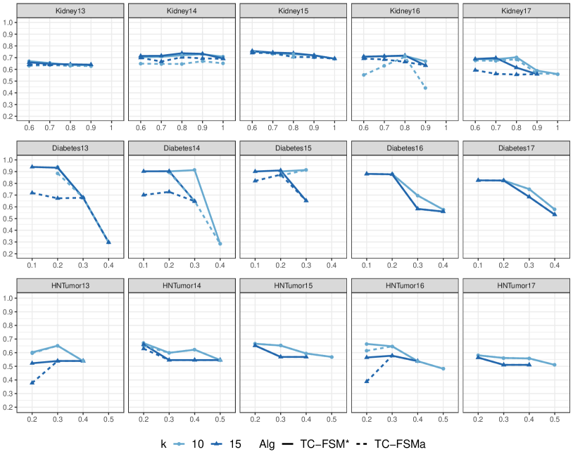
For the support threshold $\phi_{s}$, we observe overall a slight increase in the F1-scores for the Kidney and HNTumor groups when we decrease $\phi_{s}$. For the Diabetes groups, there is a considerable increase in F1-scores during the beginning (when $\phi_{s}$ is decreased from 0.4 to 0.2), but this improvement also fades out. One reason for this is because when the support threshold is low, more patterns are found and used as criteria; thus, more patients are included in the cluster including false positives. While the recall increases, the precision becomes lower, which led to a small increase in the F1-scores. For the diabetes group, when the support $\phi_{s}$ is 0.4, the number of sequence patterns is extremely small (1 or 3). When the support decreases, it allowed the algorithm to find a consider number of defining patterns that is significant to retrieve the patients of the ground truth clusters. This increases the recall dramatically without a significant decrease in precision. Furthermore, Fig. 3 also shows that using fewer training samples ($k=10$, denoted using light blue), our approach can achieve the same scores as when using a larger training sample set ($k=15$, denoted using darker blue). In many cases, the former (i.e., $k=10$) even achieved a better result. This may be due to that the training test set $P\backslash P_{tr}$ is larger.

5.2.2 EO2) Comparing the F1-scores achieved.

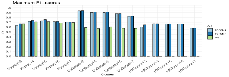
We write TC-FSM* to refer to the maximum score of our approach using the above settings. We write TC-FSM1 to denote our approach with a single setting (0.8 for kidney, 0.2 for diabetes, and 0.2 for NH-tumor, with sample size 30 and $k_{tr}=10$), to compare our results to the previous work [6]. The parameters are selected on the results of EO1. We write FIS for referring to the previous approach that uses frequent item sets [6].

Fig. 4 shows the maximum F1-scores of TC-FSM*, TC-FSM1, and FIS on the 15 clusters over 5 years and three groups. For the diabetes group, we achieved a considerable improvement of 0.2-0.3 in the F1-scores, compared to the FIS approach [6]. Overall, our approach achieved a better result. One reason for this improvement is with the use of sequential patterns (instead of frequent item sets), our approach is able to decrease the number of false positives and find the clusters with a higher precision.

Figure 4: F1-measures achieved by our approaches TC-FSM1 and TC-FCM^∗ for the three groups, compared to the ones achieved by the previous approach FIS [6].

5.2.3 EO3) Frequent Sequence Patterns to Simple Process Maps.

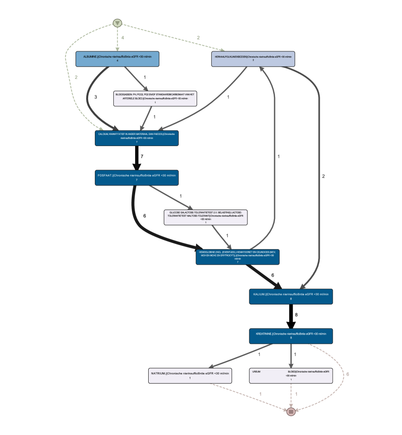
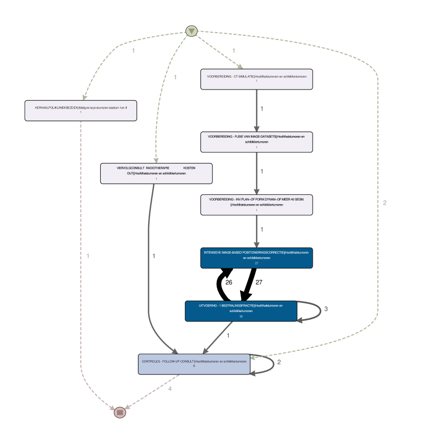
We used the closed sequence patterns mined on the samples as the traces that represent the frequent behavior shared by the group. Using these sequence patterns, the discovered process maps overall seem to be simple and insightful, representing only the crucial behavioral criteria of the patient groups. We show three process maps in Fig. 5, Fig. 6 and Fig. 7, for $C_{kidney17}$, $C_{HNTumor16}$, and $C_{Diabetes16}$ to illustrate our results. All the process maps contain all activities and paths (thus no filters applied). As can be seen in Fig. 5, the number of activity labels in the process is reduced from about 4,700 to 11. The number of distinct variants is reduced from 140 to 8.

The process maps are shown to the semi-medical expert and the data analyst. The semi-medical expert observes and confirms that the activities shown (e.g., “kalium” (potassium), “kreatinine” (creatinine), “calcium” (calcium), “fosfaat” (phosphate), “albumine” (albumin), “natrium” (sodium), “ureum bloed” (ureum blood), etc.) are important activities (e.g., lab activities) in the clinical pathway of the kidney groups (patients with renal insufficiency). The data analyst confirms that the diagnosis code “Chronic renal failure eGFR $<30$ ml/min” associated with these activities is a crucial criteria for defining the kidney groups.

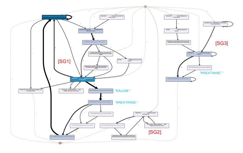
In Fig. 6 and Fig. 7, we also observe that multiple distinct diagnosis codes are used for the HNTumor and diabetes group, respectively. In the process map for $C_{Diabetes16}$, we found the process map being divided into three sub processes based on the diagnosis codes: [SG1] “diabetes mellitus without secondary complications”, [SG2] “diabetes mellitus with secondary complications”, and [SG3] “diabetes mellitus chronic pump therapy” (see Fig. 7, highlighted in red).

The semi-medical expert also observes and confirms that some of these activities are important indicators for different groups. For example, “creatinine” is important for both the kidney and diabetes groups. Nevertheless, because our approach is able to combine and handle the activities with their diagnosis codes as activity labels (in terms of the large variety of distinct labels and process variants), it enabled us to accurately distinguish the “creatinine” for the kidney group (i.e., “creatinine$||$Chronic renal failure eGFR $<30$ ml/min”) versus the same “creatinine” but for the diabetes group (i.e., “creatinine$||$SG1” and “creatinine$||$SG3”, see Fig. 7, highlighted in blue).

Figure 5: The full process map based on the closed FSPs of the kidney group;  600 activities are reduced to 11 labels.

Figure 6: The full process map based on the closed FSPs of the HNTumor group.

Figure 7: The full process map based on the closed FSPs of the diabetes group; three distinct subgroups SG1, SG2, and SG3 are found.

5.3 Discussion

The results have shown that our approach using the discovered and selected frequent sequence patterns can help to cluster the patient groups with a reasonably high accuracy (e.g., a maximum of 0.75 for the Kidney group, 0.94 for Diabetes, and 0.67 for HNTumor), despite the very large data sets (on average, about 130,000 of patients and $3.9$ millions of events per year) and the relatively very small and unbalanced clusters. Moreover, the proposed approach that automatically determines the parameters achieved F1-scores that are very close to the optimal scores. This means after setting the support $\phi_{s}$ and with no further input, we can find the clusters with a reasonable quality as well. Using the process maps, we show the meaningful and insightful behavioral patterns and criteria in the clinical pathways of the patient groups. According to the semi-medical expert, the maps can be a useful tool in the communication with the domain experts regarding the pathways. Note that we do not have any prior knowledge of the specific activities or diagnosis codes of the patient groups.

A remark is that these process maps of FSPs have a different semantics than the formal process models discovered using the traces. For example, an edge from A to B in the map, in essence, means that such an eventually-followed relation is frequent. To obtain formal models, we may project the patterns on the traces and use the instances of the patterns in the traces to discover models [18].

6 Conclusion and Future Work

In this paper, we investigated the trace clustering problem in healthcare and proposed an approach that can handle the characteristics of healthcare data. Using a small sample set of patients, the proposed approach finds frequent sequence patterns and uses these as behavioral criteria for determining a cluster. The results of the evaluations show that the approach is able to identify patient clusters with a very reasonable quality on the basis of very limited input from medical experts, despite the very large data sets and the small, unbalanced clusters (ground-truth). The obtained behavioral criteria also led to the generation of simple process maps, where we have some first insights that these could be actually used by medical experts. The semi-medical expert who works closely with medical experts was able to recognize the important activities in the clinical pathways of the patient groups. Such a method may be useful to reason about clinical pathways within hospitals for the sake of process improvement or quality control.

For future work, we plan to investigate other strategies for selecting sequence patterns as behavioral criteria to further improve the F1-scores. Also, the effect of sample size on the F1-scores is worth investigating. Another interesting direction is to exploit the frequent sequence patterns to discover formal process models for the clinical pathways of each cluster. Finally, we would like to validate the maps with medical experts and apply our approach to other patient clusters and other hospitals.

Acknowledgments. This research was supported by the NWO TACTICS project (628.011.004) and Lunet Zorg in the Netherlands. We would also like to thank the experts from the VUMC for their extremely valuable assistance and feedback in the evaluation.

References

- [1] Rojas, E., Munoz-Gama, J., Sepúlveda, M., Capurro, D.: Process mining in healthcare: A literature review. Journal of Biomedical Informatics 61 (2016) 224–236
- [2] Caron, F., Vanthienen, J., Vanhaecht, K., van Limbergen, E., De Weerdt, J., Baesens, B.: Monitoring care processes in the gynecologic oncology department. Comp. in Bio. and Med. 44 (2014) 88–96
- [3] Greco, G., Guzzo, A., Pontieri, L., Saccà, D.: Discovering expressive process models by clustering log traces. IEEE Trans. Knowl. Data Eng. 18(8) (2006) 1010–1027
- [4] De Weerdt, J., vanden Broucke, S.K.L.M., Vanthienen, J., Baesens, B.: Active trace clustering for improved process discovery. IEEE Trans. Knowl. Data Eng. 25(12) (2013) 2708–2720
- [5] Schreyögg, J., Stargardt, T., Tiemann, O., Busse, R.: Methods to determine reimbursement rates for diagnosis related groups (drg): a comparison of nine european countries. Health care management science 9(3) (2006) 215–223
- [6] Tabatabaei, S.A., Lu, X., Hoogendoorn, M., Reijers, H.A.: Identifying patient groups based on frequent patterns of patient samples. CoRR abs/1904.01863 (2019)
- [7] Song, M., Günther, C.W., van der Aalst, W.M.P.: Trace clustering in process mining. In: BPM 2008 International Workshops, Milano, Italyy, 2008. (2008) 109–120
- [8] Bose, R.P.J.C., van der Aalst, W.M.P.: Trace clustering based on conserved patterns: Towards achieving better process models. In: BPM 2009 International Workshops, September 7, 2009. Revised Papers. (2009) 170–181
- [9] Bose, R.P.J.C., van der Aalst, W.M.P.: Context aware trace clustering: Towards improving process mining results. In: SDM 2009, Proceedings. (2009) 401–412
- [10] Chatain, T., Carmona, J., van Dongen, B.F.: Alignment-based trace clustering. In: ER. Volume 10650 of Lecture Notes in Computer Science., Springer (2017) 295–308
- [11] Cadez, I.V., Heckerman, D., Meek, C., Smyth, P., White, S.: Model-based clustering and visualization of navigation patterns on a web site. Data Min. Knowl. Discov. 7(4) (2003) 399–424
- [12] Ferreira, D.R., Zacarias, M., Malheiros, M., Ferreira, P.: Approaching process mining with sequence clustering: Experiments and findings. In: BPM 2007, Proceedings. (2007) 360–374
- [13] De Koninck, P., Nelissen, K., Baesens, B., vanden Broucke, S., Snoeck, M., De Weerdt, J.: An approach for incorporating expert knowledge in trace clustering. In: CAiSE 2017, Proceedings. (2017) 561–576
- [14] Fumarola, F., Lanotte, P.F., Ceci, M., Malerba, D.: Clofast: closed sequential pattern mining using sparse and vertical id-lists. Knowl. Inf. Syst. 48(2) (2016) 429–463
- [15] Fournier-Viger, P., Gomariz, A., Gueniche, T., Soltani, A., Wu, C., Tseng, V.S.: SPMF: a java open-source pattern mining library. Journal of Machine Learning Research 15(1) (2014) 3389–3393
- [16] Ceci, M., Spagnoletta, M., Lanotte, P.F., Malerba, D.: Distributed learning of process models for next activity prediction. In: IDEAS, ACM (2018) 278–282
- [17] Lee, W.S., Liu, B.: Learning with positive and unlabeled examples using weighted logistic regression. In: ICML. Volume 3. (2003) 448–455
- [18] Lu, X., Fahland, D., Andrews, R., Suriadi, S., Wynn, M.T., ter Hofstede, A.H.M., van der Aalst, W.M.P.: Semi-supervised log pattern detection and exploration using event concurrence and contextual information. In: OTM Conferences (1) - COOPIS. (2017) 154–174