Parameter learning and fractional differential operators: application in image regularization and decomposition

Abstract

In this paper, we focus on learning optimal parameters for PDE-based image regularization and decomposition. First we learn the regularization parameter and the differential operator for gray-scale image denoising using the fractional Laplacian in combination with a bilevel optimization problem. In our setting the fractional Laplacian allows the use of Fourier transform, which enables the optimization of the denoising operator. We prove stable and explainable results as an advantage in comparison to other machine learning approaches. The numerical experiments correlate with our theoretical model setting and show a reduction of computing time in contrast to the ROF model. Second we introduce a new image decomposition model with the fractional Laplacian and the Riesz potential. We provide an explicit formula for the unique solution and the numerical experiments illustrate the efficiency.

1 Introduction

In the last few years machine learning approaches have been established in image processing and computer vision. In contrast to this, variational regularization methods are used in image processing and computer vision since decades. Variational regularization techniques offer rigourous and comprehensible image analysis, which allows stable numerical results and error estimates. The certainty of giving explainable results is essential in a broad field of applications. Machine learning methods, on the other hand, are extremly powerful as they learn directly from datas for a specific task. The weak point of data-driven approaches is that they generally cannot offer stability or error bounds. In this paper we want to combine machine learning and variational regularization techniques. In particular, we learn optimal image regularizers and data fidelity parameters via a bilevel optimization approach making use of a training set. One of the central problems in image processing is denoising. Total variation image denoising is done with the so-called Rudin-Osher-Fatemi (ROF) model RudOshFat92 , which seeks a minimizer $u\in BV({\mathds{T}^{d}})\cap L^{2}({\mathds{T}^{d}})$ for

$$\hskip 28.45274ptE(u)=\big{|}Du\big{|}_{{\mathds{T}^{d}}}+\frac{\alpha}{2}\lVert g-u\rVert^{2}.$$

The $d$-dimensional torus ${\mathds{T}^{d}}$ denotes the image domain, $\lVert\cdot\rVert$ is the norm in $L^{2}({\mathds{T}^{d}},\mathbb{C})$, and $\alpha$ is a regularization parameter. The function $g:{\mathds{T}^{d}}\rightarrow\mathbb{C}$ represents the given image, which typically contains noise. A numerical difficulty of the ROF model is the non-differentiability of the total variation term. In the last years the use of differential operators, which involves fractional powers, were applied on many different kinds of problems, for example in frak1 . In image denoising as an alternative to the ROF model the total variation term is replaced by the fractional Laplacian. Fractional Laplacian denoising of an image is given by minimizing

$$E(u)=\frac{1}{2}\lVert(-\Delta)^{\frac{s}{2}}u\rVert^{2}_{{L^{2}({\mathds{T}^{d}};\mathbb{C})}}+\frac{\alpha}{2}\lVert u-g\rVert^{2}_{{L^{2}({\mathds{T}^{d}};\mathbb{C})}}.$$

The application of the fractional Laplacian in image denoising has been done in AntBar17 . The results of this fractional model has a computing time, which is a reduction by factors 10-100 in contrast to the well-known ROF model. Also in cguys and disantil the fractional Laplacian has been used in image denoising and got comparable results to the ROF model. Independent of the concrete choice of the model, the main issue in image regularization is the choice of particular regularization parameters, in our case the two parameters $s$ and $\alpha$. A well-known approach to compute suitable parameters is to define a bilevel optimization problem. A bilevel approach regarding a $TV_{p}$-image denoising model is studied in LiuSch19 . But the authors point out, that their scheme is numerically inefficient. To find the optimal regularization parameters they discretize the parameter interval and iterate over every grid point. An alternative approach using the fractional Laplacian is done in AntKha19 . There the authors learn the parameters via a so called Bilevel Optimization Neural Network. But as a disadvantage, which is typical for Neural Networks, no error estimates for the solutions are available.

1.1 Contribution of this work

In this paper we obtain an image denoising model using the fractional Laplacian, which is on the one hand numerically fast to compute and on the other hand analytically understandable. We prove rigorous error estimates for the continous and the discrete solution. We consider the case of supervised learning. This means we are given noisy images $g$ and the corresponding noise-free image $u_{d}$. For simplicity we perform our model on a single pair $(g,u_{d})$, but for multiple image pairs the results are a straightforward modification. The main idea of our model is to learn the optimal parameters $s$ and $\alpha$ on training data. The bilevel optimization problem is defined via

$$\min J(s,\alpha,u)=\frac{1}{2}\lVert u-u_{d}\rVert^{2}+\varphi(s,\alpha)$$

$$\text{s.t. }(-\Delta)^{s}u+\alpha u=\alpha g\text{ in }{\mathds{T}^{d}}$$

$$\text{with }(s,\alpha)\in W.$$

The properties and the role of the function $\varphi$ will be discussed later. A theoretical analysis of this type of optimization problem in a more general setting is found in Sprekel . In the second part of the paper we apply fractional differential operators in image decomposition. We consider a novel image decomposition model of the form

$$\hskip 28.45274ptI(u,v) =\frac{1}{2}\lVert(-\Delta)^{\frac{s_{1}}{2}}u\rVert^{2}+$$

$$\frac{\alpha}{2}\lVert u+v-g\rVert^{2}+\frac{\beta}{2}\lVert R_{\frac{s_{2}}{2}}(v)\rVert^{2}.$$

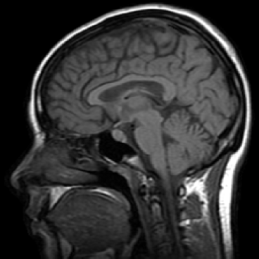
(a)

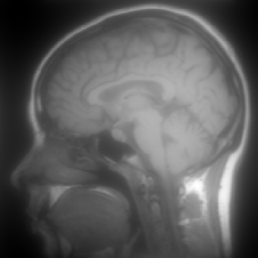
(b)

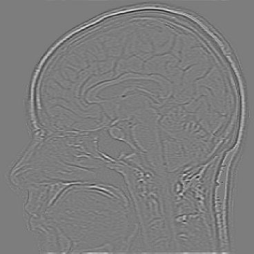
(c)

Figure 1: Decomposition of the original image (left) in structural component $u$ (middle) and textural component $v$ (right)

Typically the structural component $u$ contains the main components of the image, which is represented by the lower frequencies. The textural component $v$ contains the finer details like edges or high oscillations. These components are included in the high frequencies of an image. Therefore we introduce the Riesz potential, which captures the high frequencies, as the inverse of the fractional Laplacian. In Figure 1 we illustrate a decomposition into these components. This paper contains two main results. First we derive a rigourous error estimate for the bilevel problem in the case of spectral approximation. The numerical realization is easy to implement and in comparison to the ROF model much faster. Second we introduce a new image decomposition model, which has promising results in simultaneous image denoising and decomposition. To the best of our knowledge, this is the first work using fractional models in image decomposition. Moreover, we point out, that fractional differential operators are applicable in case of image denoising and decompositon. The use of fractional diffential operators in other image processing areas is a point of future research.

1.2 Overview

This paper is organized as follows: In Section 2 we recall some facts about fractional Sobolev spaces and spectral approximation. The use of the fractional Laplacian in a bilevel image denoising approach is topic of Section 3. Afterwards in Section 4 a spectral approximation of this problem is introduced. In Section 5 we discuss the numerical experiments. An image decomposition approach is done in Section 6 with numerical experiments in Section 7.

2 Fractional Sobolev spaces and spectral approximation

In this paragraph we collect some well known results concering fractional Sobolev spaces and spectral approximation. We follow AntBar17 .

2.1 Fractional Sobolev spaces

On the torus ${\mathds{T}^{d}}$ the Laplacian operator
$-\Delta:H^{2}_{0}({\mathds{T}^{d}};\mathbb{C})\rightarrow{L^{2}_{0}({\mathds{T}^{d}};\mathbb{C})}$ is defined via

$$\hskip 28.45274pt-\Delta u=\frac{1}{(2\pi)^{d}}\sum\limits_{k\in\mathbb{Z}^{d}\setminus\{0\}}|k|^{2}\hat{u}_{k}\varphi^{k}.$$

with the functions $\varphi^{k}(x)=e^{ik\cdot x}$ and $\hat{u}_{k}=\\ (u,\varphi^{k})_{L^{2}({\mathds{T}^{d}};\mathbb{C})}$. In this setting the Laplacian operator is unbounded, non-negativ, self-adjoint and bijective. Therefore we can apply the theorem ”Operators with compact inverses” (BoyFab13 , Theorem II-6.6). As a result we can characterize the domain of the Laplacian as

$$D(-\Delta)=H^{2}_{0}({\mathds{T}^{d}};\mathbb{C})=$$

$$\{u\in{L^{2}_{0}({\mathds{T}^{d}};\mathbb{C})}~{}\big{|}\sum\limits_{k\in\mathbb{Z}^{d}\setminus\{0\}}|k|^{4}|\hat{u}_{k}|^{2}<\infty\}.$$

Using this spectral decomposition we can define the fractional Sobolev spaces with $0\leq s\leq 1$ as

$$H^{s}_{0}({\mathds{T}^{d}};\mathbb{C}):=$$

$$\Big{\{}u\in{L^{2}_{0}({\mathds{T}^{d}};\mathbb{C})}~{}\big{|}\sum\limits_{k\in\mathbb{Z}^{d}\setminus\{0\}}|k|^{4s}|\hat{u}_{k}|^{2}<\infty\Big{\}}.$$

The next theorem gives us analogous embeddings as in the case of general Sobolev spaces.

Theorem 2.1 (Rellich’s theorem on ${\mathds{T}^{d}}$)

For all $0\leq s<s^{\prime}$ we have $H^{s^{\prime}}_{0}({\mathds{T}^{d}};\mathbb{C})\subset H^{s}_{0}({\mathds{T}^{d}};\mathbb{C})$.
Moreover, the canonical embedding is compact.

Proof

BoyFab13 Proposition II.6.8. ∎

The fractional Sobolev spaces are the natural setting to generalize the Laplacian operator on the torus.

Definition 1 (Fractional Laplacian)

For $s>0$ we define the fractional Laplacian $(-\Delta)^{s}$, applied on $u\in H^{s}_{0}({\mathds{T}^{d}};\mathbb{C})$, as

$$\hskip 28.45274pt(-\Delta)^{s}u=\frac{1}{(2\pi)^{d}}\sum\limits_{k\in\mathbb{Z}^{d}}|k|^{2s}\hat{u}_{k}\varphi^{k}.$$ (1)

(a) $(-\Delta)^{0}u_{d}=id~{}u_{d}$

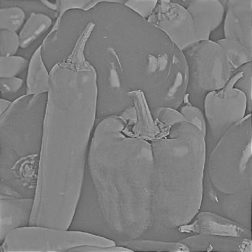
(b) $(-\Delta)^{\frac{1}{3}}u_{d}$

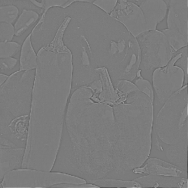
(c) $(-\Delta)^{\frac{2}{3}}u_{d}$

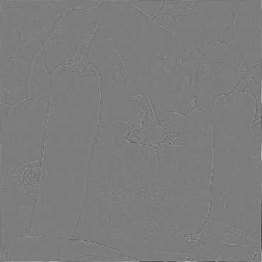
(d) $(-\Delta)^{1}u_{d}=-\Delta u_{d}$

Figure 2: Fractional Laplacian (1) of image $u_{d}$. A higher exponent $s$ in (1) emphasizes stronger the high oscillations.

The fractional Laplacian is a linear operator for the argument $u$, but non-linear in the parameter $s$. Moreover we can define fractional Sobolev spaces for negative $s$. The domain $D((-\Delta)^{s})$ of the fractional Laplacian with $s<0$ must fullfill the property of being a super set from ${L^{2}_{0}({\mathds{T}^{d}};\mathbb{C})}$; so we modify the norm for negative $s$ with

$$\hskip 28.45274pt\lVert u\rVert^{2}_{D((-\Delta)^{s})}:=\sum\limits_{k\in\mathbb{Z}^{d}\setminus\{0\}}|k|^{4s}|\hat{u}_{k}|^{2}.$$

Definition 2 (Negative Sobolev spaces)

Let $s<0$. We refer $\dot{H}^{s}({\mathds{T}^{d}};\mathbb{C})$ as the negative Sobolev spaces defined as the completition of ${L^{2}_{0}({\mathds{T}^{d}};\mathbb{C})}$ regarding the norm $\lVert\cdot\rVert_{D((-\Delta)^{s})}$.

It can be shown that $\dot{H}^{s}({\mathds{T}^{d}};\mathbb{C})$ is a Hilbert space with the scalar product

$$\hskip 28.45274pt(u,v)_{\dot{H}^{s}({\mathds{T}^{d}};\mathbb{C})}=\sum\limits_{k\in\mathbb{Z}^{d}\setminus\{0\}}|k|^{2s}\hat{u}_{k}\overline{\hat{v}_{k}}.$$

We are now in a position to define the Riesz potential, which is the negative analogue to the fractional Laplacian.

Definition 3 (Riesz potential)

For $s\leq 0$ we define the Riesz potential of a function
$u\in\dot{H}^{s}({\mathds{T}^{d}};\mathbb{C})$ as the inverse of the fractional Laplacian with

$$\hskip 28.45274ptR_{s}(u)=\frac{1}{(2\pi)^{d}}\sum\limits_{k\in\mathbb{Z}^{d}\setminus\{0\}}|k|^{2s}\hat{u}_{k}\varphi^{k}.$$ (2)

(a) original image $u_{d}$

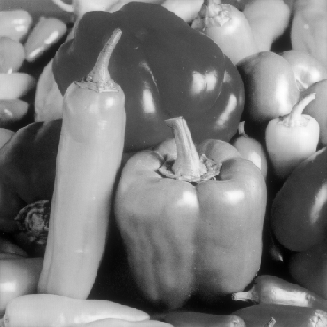
(b) $R_{-0.1}(u_{d})$

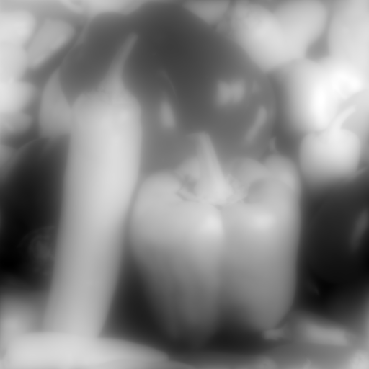
(c) $R_{-0.5}(u_{d})$

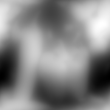
(d) $R_{-0.9}(u_{d})$

Figure 3: Riesz potential (2) of image $u_{d}$. A lower exponent $s$ in (2) smooths the image $u_{d}$.

2.2 Spectral approximation

For short summaries about spectral approximation, we refer to AntBar17 and spec . The space of trigonometric polynomials on the torus ${\mathds{T}^{d}}$ is defined via

$$\hskip 28.45274pt\mathcal{T}_{n} =\Big{\{}v_{n}\in C({\mathds{T}^{d}},\mathbb{C})~{}$$

$$\big{|}~{}v_{n}(x)=\sum\limits_{k\in\mathbb{Z}^{d}_{n}}c_{k}\varphi^{k}(x),c_{k}\in\mathbb{C}\Big{\}},$$

with $\mathbb{Z}^{d}_{n}:=\{k\in\mathbb{Z}^{d}~{}~{}\big{|}\frac{-n}{2}\leq k_{i}\leq\frac{n}{2}-1~{}\forall i\}$. The functions $\varphi^{k}(x)=e^{ik\cdot x}$ define an orthogonal basis in $\mathcal{T}_{n}$ regarding the $L^{2}$-scalar product.
With $v$ we associate a grid function $\textbf{V}=(v_{j}|~{}j\in\mathbb{N}^{d}_{n})$, which is represented by

$$\hskip 28.45274ptv_{j}=v(x_{j})\text{ , }x_{j}=\frac{2\pi}{n}(j_{1},...,j_{d}),$$

$$\hskip 28.45274ptj\in\mathbb{N}^{d}_{n}=\{~{}j\in\mathbb{N}^{d}~{}|~{}0\leq j_{i}\leq n-1~{}\forall j\}.$$

The discrete scalar product of two grid functions $\textbf{V}=(v_{j}~{}|~{}j\in\mathbb{N}^{d}_{n})$ and $\textbf{W}=(w_{j}~{}|~{}j\in\mathbb{N}^{d}_{n})$ is given by

$$\hskip 28.45274pt(\textbf{V},\textbf{W})_{n}:=\frac{(2\pi)^{d}}{n^{d}}\sum_{j\in\mathbb{N}^{d}_{n}}v_{j}\bar{w}_{j}.$$

The induced norm is denoted by $\|\cdot\|_{n}$.

Definition 4 (Fourier transform)

For a given grid function $\textbf{V}=(v_{j}~{}|~{}j\in\mathbb{N}^{d}_{n})$ the discrete Fourier transform is defined as the coefficient vector $\tilde{\textbf{V}}=(\tilde{v}_{k}|~{}k\in\mathbb{Z}^{d}_{n})$ with

$$\hskip 28.45274pt\tilde{v}_{k}=(V,\Phi^{k})_{n}.$$

The family

$$\hskip 28.45274pt\Phi^{k}=(e^{ik\cdot x_{j}}~{}|~{}j\in\mathbb{N}^{d}_{n})~{},~{}x_{j}=\frac{2\pi}{n}(j_{1},...,j_{d})$$

defines an orthogonal basis in the space of grid functions regarding $(\cdot,\cdot)_{n}$.

To approximate a function in the fractional
Sobolev space $H^{s}_{0}({\mathds{T}^{d}};\mathbb{C})$, we consider suitable approximation in the trigonometric space $\mathcal{T}_{n}$.

Definition 5 (Orthogonal projection)

The projection $P_{n}:{L^{2}({\mathds{T}^{d}};\mathbb{C})}\rightarrow\mathcal{T}_{n}$ fulfills for all $v\in{L^{2}({\mathds{T}^{d}};\mathbb{C})}$ the property

$$\hskip 28.45274pt(P_{n}v,w_{n})=(v,w_{n})~{}~{}~{}\forall w_{n}\in\mathcal{T}_{n}.$$

Using the orthogonality of the basis functions we get

$$\hskip 28.45274ptP_{n}v=\sum\limits_{k\in\mathbb{Z}^{d}_{n}}\hat{v}_{k}\varphi^{k}.$$

The discrete Fourier transformation allows us to define a suitable trigonometric interpolation.

Definition 6 (Trigonometric interpolant)

Given $v\in C({\mathds{T}^{d}};\mathbb{C})$ and discrete Fourier coefficients $\tilde{\textbf{V}}=(\tilde{v}_{k}~{}|~{}k\in\mathbb{Z}^{d}_{n})$, the trigonometric interpolant $I_{n}v\in\mathcal{T}_{n}$ of $v$ is defined via

$$\hskip 28.45274ptI_{n}v=\frac{1}{(2\pi)^{d}}\sum_{k\in\mathbb{Z}^{d}_{n}}\tilde{v}_{k}\varphi^{k}.$$

The following error estimate can be found in AntBar17 . The norm $\lVert\cdot\rVert_{D((-\Delta)^{s})}$ is denoted by $|\cdot|_{s}$.

Lemma 1 (Projection error)

For $\gamma_{1},\gamma_{2}\in\mathbb{R}$ with $\gamma_{1}\leq\gamma_{2}$ and $v\in H^{\gamma_{2}}_{0}({\mathds{T}^{d}};\mathbb{C})$ we obtain

$$\hskip 28.45274pt|v-P_{n}v|_{\gamma_{1}}\leq\Big{(}\frac{n}{2}\Big{)}^{-(\gamma_{2}-\gamma_{1})}|v|_{\gamma_{2}}.$$

Lemma 2 (Interpolation error)

If $\gamma_{2}>\frac{d}{2},0\leq\gamma_{1}\leq\gamma_{2}$ and $v\in H^{\gamma_{2}}_{0}({\mathds{T}^{d}};\mathbb{C})$ we obtain

$$\hskip 28.45274pt|v-I_{n}v|_{\gamma_{1}}\leq c_{d,\gamma_{1},\gamma_{2}}\Big{(}\frac{n}{2}\Big{)}^{-(\gamma_{2}-\gamma_{1})}|v|_{\gamma_{2}}$$

with a constant $c_{d,\gamma_{1},\gamma_{2}}>0$ independent of $v$ and $n$.

3 Application of fractional Laplacian in bilevel image optimization

As mentioned in the introduction for a given noisy image $g\in{L^{2}({\mathds{T}^{d}};\mathbb{C})}$ we want to solve

$$\hskip 14.22636pt\min~{}E(u)=\frac{1}{2}\lVert(-\Delta)^{\frac{s}{2}}u\rVert^{2}+\frac{\alpha}{2}\lVert u-g\rVert^{2}$$ (3)

with $0<s<1$ and $u\in H^{s}_{0}({\mathds{T}^{d}};\mathbb{C})\cap{L^{2}_{0}({\mathds{T}^{d}};\mathbb{C})}$. The main idea of this model is to supress the high frequencies, which typically contain noise. In the following we always assume, that the mean value of $g$ is zero. Otherwise, we replace $g$ with

$$\hskip 28.45274pt\tilde{g}(x):=g(x)-\frac{1}{\big{|}{\mathds{T}^{d}}\big{|}}\int_{{\mathds{T}^{d}}}g(x)~{}dx.$$

and add the mean value to the solution. As a result we can minimize in the function space $H^{s}_{0}({\mathds{T}^{d}};\mathbb{C})$. Existence and uniqueness of the solution $u$ considered in the frequency space yields

$$\hskip 28.45274ptu=\frac{1}{(2\pi)^{d}}\sum\limits_{k\in\mathbb{Z}^{d}\setminus\{0\}}\frac{\alpha}{|k|^{2s}+\alpha}\,\hat{g}_{k}\varphi^{k}.$$ (4)

(a) original image $u_{d}$

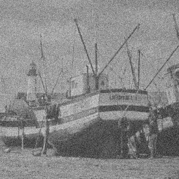
(b) noisy image $g$

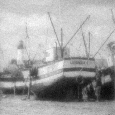
(c) $s=0.4,~{}\alpha=5$

(d) $s=0.1,~{}\alpha=1$

Figure 4: The denoising via solving (3) strongly depend on the choice of the parameters $s$ and $\alpha$.

A key point in image denoising is the choice of the parameters, in this case $s$ and $\alpha$. Normally this is done manually, which is time-consuming. As seen in Figure 4 the results of denoising an image highly depends on the right choice of the regularization parameters. To overcome this problem we use a bilevel optimization approach. We assume, that we have the original image $u_{d}\in{L^{2}({\mathds{T}^{d}};\mathbb{C})}$ and the noisy image $g$. So we define the optimization problem

$$\min_{s,\alpha,u} ~{}J(s,\alpha,u)=\frac{1}{2}\lVert u-u_{d}\rVert_{{L^{2}({\mathds{T}^{d}};\mathbb{C})}}^{2}+\varphi(\alpha,s)$$

$$\text{s.t. }(-\Delta)^{s}u+\alpha u=\alpha g$$ (5)

$$\text{with }(s,\alpha)\in W:=[s_{0},s_{1}]\times[\alpha_{0},\alpha_{1}].$$

The function $\varphi$ must fulfill following assumptions.

Definition 7

The function $\varphi\in C^{2}(W^{\mathrm{o}},\mathbb{R})$ is non negative, convex and has following properties:

$$\hskip 28.45274pt\lim\limits_{s\rightarrow s_{0}}\varphi(s,\alpha)=\lim\limits_{\alpha\rightarrow\alpha_{0}}\varphi(s,\alpha)=\infty$$

$$\hskip 28.45274pt=\lim\limits_{s\rightarrow s_{1}}\varphi(s,\alpha)=\lim\limits_{\alpha\rightarrow\alpha_{1}}\varphi(s,\alpha).$$ (6)

Parsevals’s identity and the isometry properties between ${L^{2}({\mathds{T}^{d}};\mathbb{C})}$ and $\ell^{2}(\mathbb{Z}^{d})$ imply the equivalent representation of (5) with

$$J(s,\alpha,u)=\frac{1}{2(2\pi)^{d}}\lVert\widehat{\textbf{U}}-\widehat{\textbf{U}}_{d}\rVert_{l^{2}}^{2}+\varphi(\alpha,s)$$ (7)

$$\text{s.t. }((\alpha+|k|^{2s})\hat{u}_{k}-\alpha\hat{g_{k}})_{k\in\mathbb{Z}^{d}\setminus\{0\}}=0$$ (8)

$$\text{with }(s,\alpha)\in W:=[s_{0},s_{1}]\times[\alpha_{0},\alpha_{1}].$$

The expressions $\widehat{\textbf{U}}$ and $\widehat{\textbf{U}}_{d}$ denote the Fourier coefficient vector of $u$ and $u_{d}$. Solving (8) according to $\hat{u}_{k}$ yields a solution operator $\mathcal{S}$ defined via

$$\mathcal{S}:[s_{0},s_{1}]\times[\alpha_{0},\alpha_{1}]\rightarrow\ell^{2}(\mathbb{Z}^{d})$$

$$(s,\alpha)\mapsto\mathcal{S}(s,\alpha)=\widehat{\textbf{U}}=\big{(}\frac{\alpha}{\alpha+|k|^{2s}}\hat{g_{k}}\big{)}_{k\in\mathbb{Z}^{d}}.$$ (9)

To analyze the optimization problem (7)-(8), we need to characterize the partial derivatives of the solution operator $\mathcal{S}$.

Theorem 3.1

The operator $\mathcal{S}$ as an operator from $W\rightarrow{L^{2}({\mathds{T}^{d}};\mathbb{C})}\simeq\ell^{2}(\mathbb{Z}^{d})$ is twice Fréchet-differentiable and in particular continous. For $h_{1},h_{2}\in\mathbb{R}$ the partial derivatives up to order two are represented by

$$\hskip 28.45274pt\partial_{s}\mathcal{S}(s,\alpha)[h_{1}]=h_{1}\partial_{s}\mathcal{S}(s,\alpha),$$

$$\hskip 28.45274pt\partial^{2}_{s}\mathcal{S}(s,\alpha)[h_{1},h_{2}]=h_{1}h_{2}\partial_{s^{2}}\mathcal{S}(s,\alpha),$$

$$\hskip 28.45274pt\partial_{\alpha}\mathcal{S}(s,\alpha)[h_{1}]=h_{1}\partial_{\alpha}\mathcal{S}(s,\alpha),$$

$$\hskip 28.45274pt\partial^{2}_{\alpha}\mathcal{S}(s,\alpha)[h_{1},h_{2}]=h_{1}h_{2}\partial_{\alpha^{2}}\mathcal{S}(s,\alpha),$$

$$\hskip 28.45274pt\partial_{\alpha,s}\mathcal{S}(s,\alpha)[h_{1},h_{2}]=h_{1}h_{2}\partial_{\alpha,s}\mathcal{S}(s,\alpha),$$

with

$$\partial_{s}\mathcal{S}(s,\alpha)=\sum\limits_{k\in\mathbb{Z}^{d}\setminus\{0\}}\frac{2\alpha|k|^{2s}ln(|k|)}{(|k|^{2s}+\alpha)^{2}}\hat{g}_{k},$$

$$\partial^{2}_{s}\mathcal{S}(s,\alpha)=\sum\limits_{k\in\mathbb{Z}^{d}\setminus\{0\}}\frac{4\alpha|k|^{2s}ln(|k|)^{2}(|k|^{2s}-\alpha)}{(\alpha+|k|^{2s})^{3}}\hat{g}_{k},$$

$$\partial_{\alpha}\mathcal{S}(s,\alpha)=\sum\limits_{k\in\mathbb{Z}^{d}\setminus\{0\}}\frac{|k|^{2s}}{(|k|^{2s}+\alpha)^{2}}\hat{g}_{k},$$

$$\partial^{2}_{\alpha}\mathcal{S}(s,\alpha)=\sum\limits_{k\in\mathbb{Z}^{d}\setminus\{0\}}\frac{-2|k|^{2s}}{(|k|^{2s}+\alpha)^{3}}\hat{g}_{k},$$

$$\partial_{\alpha,s}\mathcal{S}(s,\alpha)=\sum\limits_{k\in\mathbb{Z}^{d}\setminus\{0\}}\!\frac{-2|k|^{2s}ln(|k|)(|k|^{2s}-\alpha)}{(|k|^{2s}+\alpha)^{3}}\hat{g}_{k}.$$

Proof

The proof requires straightforward calculations, but follows mainly the proof structure of Section 3.1 in AntOtaSal18 . A more general case is also found in Sprekel . In our case we focus on the function $E_{k}:[s_{0},s_{1}]\times[\alpha_{0},\alpha_{1}]\rightarrow\mathbb{R}$ for $k\in\mathbb{Z}^{d}$ with

$$~{}~{}~{}~{}~{}~{}E_{k}(s,\alpha):=\frac{\alpha}{\alpha+|k|^{2s}}.$$

The remaining part of the proof is a straightforward modification of the cited paper.∎

Using the explicit representation of the partial derivatives we obtain upper bounds for these.

Lemma 3 (Boundedness of partial
derivatives)

Let $\varepsilon>0$ and $i=1,2,3$. Then we have the following estimates for the partial derivatives:

$$\hskip 28.45274pt\|\partial^{i}_{\alpha}\mathcal{S}(s,\alpha)\|_{\ell^{2}}\leq\sum\limits_{k\in\mathbb{Z}^{d}\setminus\{0\}}\frac{i!}{|k|^{2si}}|\hat{g_{k}}|,$$

$$\hskip 28.45274pt\|\partial^{i}_{s}\mathcal{S}(s,\alpha)\|_{\ell^{2}}\leq\sum\limits_{k\in\mathbb{Z}^{d}\setminus\{0\}}\frac{M_{\alpha_{1},i}}{\varepsilon^{i}|k|^{2s-i\varepsilon}}|\hat{g}_{k}|,$$

$$\hskip 28.45274pt\|\partial_{s,\alpha}\mathcal{S}(s,\alpha)\|_{\ell^{2}}\leq\sum\limits_{k\in\mathbb{Z}^{d}\setminus\{0\}}\frac{M_{\alpha_{1}}}{\varepsilon|k|^{2s-\varepsilon}}|\hat{g}_{k}|.$$

Proof

We obtain these results by using Theorem 2 and straightforward calculations.∎

If $g\in{L^{2}({\mathds{T}^{d}};\mathbb{C})}$ and $\varepsilon>0$, we deduce from Lemma  3

$$\hskip 28.45274pt\partial^{i}_{s}\mathcal{S}(s,\alpha)\in H^{2s-i\varepsilon}_{0}({\mathds{T}^{d}};\mathbb{C}),$$

$$\hskip 28.45274pt\partial^{i}_{\alpha}\mathcal{S}(s,\alpha)\in H^{2si}_{0}({\mathds{T}^{d}};\mathbb{C})$$

for $i=1,2,3$.
The introduction of the solution operator $\mathcal{S}$ allows us to consider a reduced version of (7)-(8). The reduced problem $j:\mathbb{R}^{2}\mapsto\mathbb{R}$ of (7) and (8) is given by minimizing

$$\hskip 14.22636ptj(s,\alpha) :=J(s,\alpha,\mathcal{S}(s,\alpha))$$ (10)

$$=\frac{1}{2(2\pi)^{d}}\lVert\mathcal{S}(s,\alpha)-\widehat{\textbf{U}}_{d}\rVert_{\ell^{2}}^{2}+\varphi(s,\alpha)$$

$$\text{with }(s,\alpha)\in W.$$

As an optimal triple we denote a minimizer of $j(s,\alpha)$ together with $u=\mathcal{S}(s,\alpha)$.

Definition 8 (Optimal triple)

The triple
$(\bar{s},\bar{\alpha},\mathcal{S}(\bar{s},\bar{\alpha}))\in W^{\mathrm{o}}\times H^{\overline{2s}}_{0}({\mathds{T}^{d}};\mathbb{C})$ is called optimal for the problem (5) if

$$~{}~{}~{}~{}~{}~{}j(\bar{s},\bar{\alpha})\leq j(s,\alpha)$$

for all $(s,\alpha,\mathcal{S}(s,\alpha))\in W^{\mathrm{o}}\times H^{2s}_{0}({\mathds{T}^{d}};\mathbb{C})$.

The existence of an optimal triple can easily be shown.

Theorem 3.2 (Existence of a solution)

There exists an optimal triple
$(\bar{s},\bar{\alpha},\mathcal{S}(\bar{s},\bar{\alpha}))\in W^{\mathrm{o}}\times H^{\overline{2s}}({\mathds{T}^{d}};\mathbb{C})$ for problem (5).

Proof

The proof follows AntOtaSal18 .
Let $W_{\ell}=[s_{\ell_{1}},s_{\ell_{2}}]\times[\alpha_{\ell_{1}},\alpha_{\ell_{2}}]$ be a sequence of closed intervals with $W_{\ell}\subset W_{\ell+1}\subset W^{\mathrm{o}}$ and
$\bigcup\limits_{\ell\in\mathbb{N}}W_{\ell}=W$. The continuity of $j$ guarantees the existence of

$$\hskip 28.45274pt(s_{\ell},\alpha_{\ell})=\underset{(s,\alpha)\in W_{\ell}}{\arg\,min}~{}~{}j(s,\alpha).$$

Because of the construction of the intervals we have

$$\hskip 28.45274ptj(s_{m},\alpha_{m})\leq j(s_{\ell},\alpha_{\ell})$$

for all $m\geq\ell$.
As a result we get a convergent subsequence
$\{(s_{\ell},\alpha_{\ell})\}_{\ell\in\mathbb{N}}$ with $(s_{\ell},\alpha_{\ell})\rightarrow(\bar{s},\bar{\alpha})\in W$.
The property

$$\hskip 28.45274ptj(\bar{s},\bar{\alpha})\leq j(s_{\ell},\alpha_{\ell})$$ (11)

for all $\ell\in\mathbb{N}$ and $j(s,\alpha)\geq\varphi(s,\alpha)$ together with assumption (6) yields $(\bar{s},\bar{\alpha})\in W^{\mathrm{o}}$ and the minimizer property.
Due the continuity and the closed range of $\mathcal{S}$ there exists a $\bar{\textbf{u}}$ in the image of $\mathcal{S}$ with

$$\hskip 28.45274pt\mathcal{S}(s_{\ell},\alpha_{\ell})\rightarrow\bar{\textbf{u}}=(\frac{\alpha}{\alpha+|k|^{\bar{2s}}}\hat{g}_{k})_{k\in\mathbb{Z}^{d}\setminus\{0\}}$$

for $\ell\rightarrow\infty$.
Therefore we obtain $\mathcal{S}(\bar{s},\bar{\alpha})\in H^{\overline{2s}}_{0}({\mathds{T}^{d}};\mathbb{C})$.∎

The reduced problem is essentially a restricted optimization problem in $\mathbb{R}^{2}$, so we can easily provide first order necessary and second order sufficient optimality conditions.

Theorem 3.3 (Optimality conditions)

Let $(\bar{s},\bar{\alpha},\mathcal{S}(\bar{s},\bar{\alpha}))$ be an optimal triple for problem (5). For shorter notation we define $\bar{\textbf{u}}:=\mathcal{S}(\bar{s},\bar{\alpha})$. Then the first order optimality conditions must be valid, this implies

$$\hskip 14.22636pt\frac{1}{2(2\pi)^{d}}\big{(}(\bar{\textbf{u}}-\widehat{\textbf{U}}_{d},\partial_{s}\bar{\textbf{u}})_{l^{2}}+(\partial_{s}\bar{\textbf{u}},\bar{\textbf{u}}-\widehat{\textbf{U}}_{d})_{l^{2}}\big{)}$$

$$\hskip 14.22636pt+\partial_{s}\varphi(\bar{s},\bar{\alpha})=0,$$

$$\hskip 14.22636pt\frac{1}{2(2\pi)^{d}}\big{(}(\bar{\textbf{u}}-\widehat{\textbf{U}}_{d},\partial_{\alpha}\bar{\textbf{u}})_{l^{2}}+(\partial_{\alpha}\bar{\textbf{u}},\bar{\textbf{u}}-\widehat{\textbf{U}}_{d})_{l^{2}}\big{)}$$

$$\hskip 14.22636pt+\partial_{\alpha}\varphi(\bar{s},\bar{\alpha})=0.$$

If there exists a pair $(\bar{s},\bar{\alpha})$ with $\bar{\textbf{u}}=\mathcal{S}(\bar{s},\bar{\alpha})$, which fulfills the first order optimality conditions and the Hessian matrix $\textbf{A}\in\mathbb{R}^{2\times 2}$ is positive definit, i.e.

$$\hskip 28.45274pt\det\begin{pmatrix}a_{1\,1}&a_{1\,2}\\ a_{2\,1}&a_{2\,2}\end{pmatrix}>0,$$

then $(\bar{s},\bar{\alpha},\bar{\textbf{u}})$ is an optimal triple for (5).

To get the uniqueness of the optimal tripel, we need a stronger assumption on the function $\varphi$.

Definition 9 (Strong convexity, BoyVan04 )

Let $W$ be a convex set. A two-times differentiable function $\varphi:W\subset\mathbb{R}^{n}\rightarrow\mathbb{R}$ is strongly convex, if there exists a constant $\theta>0$ with

$$\hskip 28.45274pt\nabla^{2}\varphi(x)\succeq\theta\textbf{I}$$

for all $x\in W$ , i.e. the matrix $\nabla^{2}\varphi(x)-\theta I$ is positive definit.

The definiton of strong convexity implies (cf. Nes04 )

$$\hskip 28.45274pt(\nabla\varphi(x)-\nabla\varphi(y))^{T}\big{(}x-y\big{)}\geq\theta\big{|}x-y\big{|}$$ (12)

for all $x,y\in W$ and

$$\hskip 28.45274pt\varphi(x)\geq\varphi(\bar{x})+\frac{1}{2}\theta|(x-y)|^{2}~{}~{}~{}\forall y\in W.$$ (13)

in the case $\nabla\varphi(\bar{x})=0$ for a $\bar{x}\in W$. In the following we always assume, that the function $\varphi$ is strongly convex.

Lemma 4

If $\lVert g\rVert$ and $\lVert u_{d}\rVert$ are suffienctly small, then there exists a constant $\kappa>0$, such that

$$\hskip 28.45274pt\nabla^{2}j(s,\alpha)\succeq\kappa\textbf{I}$$ (14)

for all $(s,\alpha)\in W$.

Proof

Decompose the Hessian matrix A from (3.3) in four parts with

$$x^{T}\textbf{A}x=x^{T}\textbf{M}_{1}x+x^{T}\textbf{M}_{2}x+x^{T}\textbf{M}_{3}x+x^{T}\textbf{M}_{4}x$$

for arbitrary $x\in\mathbb{R}^{2}$. The matrix $\textbf{M}_{1}$

$$\hskip 28.45274pt\textbf{M}_{1} =\frac{1}{2(2\pi)^{d}}\left(\begin{array}[]{rr}m^{1}_{11}&m^{1}_{12}\\ m^{1}_{21}&m^{1}_{22}\end{array}\right)$$

has the values

$$m^{1}_{11}=(\mathcal{S}(s,\alpha)-\widehat{\textbf{U}}_{d},\partial^{2}_{s}\mathcal{S}(s,\alpha))_{\ell^{2}},$$

$$m^{1}_{12}=m^{1}_{21}=(\mathcal{S}(s,\alpha)-\widehat{\textbf{U}}_{d},\partial^{2}_{s,\alpha}\mathcal{S}(s,\alpha))_{\ell^{2}},$$

$$m^{1}_{22}=(\mathcal{S}(s,\alpha)-\widehat{\textbf{U}}_{d},\partial^{2}_{\alpha}\mathcal{S}(s,\alpha))_{\ell^{2}}.$$

The matrix $\textbf{M}_{2}$ is defined analogously to $\textbf{M}_{1}$, only the arguments in the $\ell^{2}$-scalar-product are interchanged. Therefore the following arguments for matrix $\textbf{M}_{1}$ are also valid for matrix $\textbf{M}_{2}$. We obtain

$$\hskip 28.45274ptx^{T}\textbf{M}_{1}x=m^{1}_{11}x^{2}_{1}+2m^{1}_{12}m^{1}_{21}x_{1}x_{2}+m^{1}_{22}x^{2}_{2}$$

$$\hskip 28.45274pt\geq m^{1}_{11}x^{2}_{1}-2|m^{1}_{12}||m^{1}_{21}||x_{1}x_{2}|+m^{1}_{22}x^{2}_{2}$$

for arbitrary $x\in\mathbb{R}^{2}$. The Cauchy-Schwarz and Young inequality imply

$$\hskip 28.45274ptx^{T}M_{1}x\geq(-|m^{1}_{11}|-|m^{1}_{12}||m^{1}_{21}|)x^{2}_{1}$$

$$\hskip 28.45274pt+~{}(-|m^{1}_{22}|-|m^{1}_{12}||m^{1}_{21}|)x^{2}_{2}.$$

Together with Lemma 3 we have

$$\hskip 28.45274pt|m^{1}_{ij}|\leq\frac{C_{ij}}{s_{0}}(\lVert g\rVert+\lVert u_{d}\rVert)\lVert g\rVert.$$

The matrix $\textbf{M}_{3}$ is the Gramian matrix between the vectors $\partial_{s}\mathcal{S}(s,\alpha)$ and $\partial_{\alpha}\mathcal{S}(s,\alpha)$, which implies $x^{T}\textbf{M}_{2}x\geq 0$ for all $x\in\mathbb{R}^{2}$.
The strong convexity of the function $\varphi$ yields for the matrix $\textbf{M}_{4}$, which is defined as

$$\hskip 14.22636pt\textbf{M}_{4}=\left(\begin{array}[]{rr}\partial^{2}_{s}\varphi(s,\alpha)&\partial^{2}_{s,\alpha}\varphi(s,\alpha)\\ \partial^{2}_{s,\alpha}\varphi(s,\alpha)&\partial^{2}_{\alpha}\varphi(s,\alpha)\end{array}\right),$$

the result

$$\hskip 28.45274ptx^{T}\textbf{M}_{4}x\geq\theta|x|^{2}.$$

Combining all arguments we obtain

$$\hskip 28.45274ptx^{T}\textbf{A}x\geq-C(\lVert u_{d}\rVert,\lVert g\rVert,\frac{1}{s_{0}})|x|^{2}+\theta|x|^{2}.$$

Therefore we have for suffienctly small $\lVert u_{d}\rVert$ and $\lVert g\rVert$, that the constant $C(\lVert u_{d}\rVert,\lVert g\rVert,\frac{1}{s_{0}})$ is smaller than $\theta$. This implies the positiv definitness of the matrix A.∎

If the prerequisites of Lemma 4 are fulfilled, we obtain for an optimal triple $(\bar{s},\bar{\alpha},\mathcal{S}(\bar{s},\bar{\alpha}))$

$$\hskip 28.45274pt(\nabla j(s,\alpha)-\nabla j(\bar{s},\bar{\alpha}))^{T}\Big{(}\binom{s}{\alpha}-\binom{\bar{s}}{\bar{\alpha}}\Big{)}$$

$$\hskip 28.45274pt\geq\kappa\Big{|}\binom{s}{\alpha}-\binom{\bar{s}}{\bar{\alpha}}\Big{|}^{2}~{}~{}~{}$$

and

$$\hskip 28.45274ptj(s,\alpha)\geq j(\bar{s},\bar{\alpha})+\frac{\kappa}{2}\Big{|}\binom{\bar{s}}{\bar{\alpha}}-\binom{s}{\alpha}\Big{|}^{2}~{}~{}~{}$$

for all $(s,\alpha)\in W$. The quadratic growth conditon implies the uniqueness of the optimal triple.

4 Spectral approximation and convergence analysis

For given $g_{n}\in\mathcal{T}_{n}$ we have the discrete problem

$$~{}~{}~{}~{}~{}~{}(-\Delta)^{s}u_{n}+\alpha u_{n}=\alpha g_{n}~{}~{}\text{in}~{}\mathcal{T}_{n}.$$

Define the discrete solution operator $\mathcal{S}_{n}$ via

$$~{}~{}~{}~{}~{}\mathcal{S}_{n}:[s_{0},s_{1}]\times[\alpha_{0},\alpha_{1}]\rightarrow\mathcal{T}_{n},$$

$$~{}~{}~{}~{}~{}(s,\alpha)\mapsto(\frac{\alpha}{\alpha+|k|^{2s}}\hat{{g}}_{n,k})_{k\in\mathbb{Z}^{d}_{n}}.$$

The following Lipschitz continuity holds.

Lemma 5 (Stability)

Let $\textbf{u}=\mathcal{S}(s,\alpha)$ be the continous and $\textbf{u}_{n}=\mathcal{S}_{n}(s,\alpha)$ the discrete solution for $(s,\alpha)\in W$. Then we have the following error estimate between these both solutions

$$~{}~{}~{}~{}~{}~{}|\textbf{u}-\textbf{u}_{n}|_{s}\leq\alpha|\widehat{\textbf{G}}-\widehat{\textbf{G}}_{n}|_{-s}.$$

Proof

We have

$$\hskip 14.22636pt|\textbf{u}-\textbf{u}_{n}|_{s}^{2}=\lVert(-\Delta)^{\frac{s}{2}}(\textbf{u}-\textbf{u}_{n})\rVert^{2}_{\ell^{2}}$$

$$\hskip 14.22636pt=((-\Delta)^{s}(\textbf{u}-\textbf{u}_{n}),\textbf{u}-\textbf{u}_{n})_{\ell^{2}}$$

$$\hskip 14.22636pt=(\alpha\widehat{\textbf{G}}-\alpha\textbf{u}-\alpha\hat{\textbf{g}}_{n}+\alpha\textbf{u}_{n},\textbf{u}-\textbf{u}_{n})_{\ell^{2}}$$

$$\hskip 14.22636pt=\!\alpha(\widehat{\textbf{G}}-\widehat{\textbf{G}}_{n},\textbf{u}-\textbf{u}_{n})_{\ell^{2}}\!-\!\alpha(\textbf{u}-\textbf{u}_{n},\textbf{u}-\textbf{u}_{n})_{\ell^{2}}$$

$$\iff|\textbf{u}-\textbf{u}_{n}|_{s}^{2}+\alpha|\textbf{u}-\textbf{u}_{n}|_{0}^{2}=\alpha(\widehat{\textbf{G}}-\widehat{\textbf{G}}_{n},\textbf{u}-\textbf{u}_{n})_{\ell^{2}}.$$

For $s,r\in\mathbb{R}$ with $s\leq r$ we have the estimate

$$\hskip 28.45274pt|\widehat{\textbf{V}}|_{s}\leq|\widehat{\textbf{V}}|_{r}$$ (15)

and therefore

$$\hskip 22.76228pt|\textbf{u}-\textbf{u}_{n}|_{s}^{2}+\alpha|\textbf{u}-\textbf{u}_{n}|_{0}^{2}\leq(1+\alpha)|\textbf{u}-\textbf{u}_{n}|_{s}^{2}$$

$$\hskip 22.76228pt\leq(1+\alpha)\alpha|\widehat{\textbf{G}}-\widehat{\textbf{G}}_{n}|_{-s}|\textbf{u}-\textbf{u}_{n}|_{s},$$

which implies the assertion.∎

The discrete solution operator $\mathcal{S}_{n}$ allows us to define an approximation for the optimization problem $j$.

Definition 10

The discrete optimization problem $j_{n}$ with $n\in\mathbb{N}$ is defined as

$$\hskip 28.45274pt\min_{(s,\alpha)\in W}j_{n}(s,\alpha)$$ (16)

$$\hskip 28.45274pt=\frac{1}{2(2\pi)^{d}}\lVert S_{n}(s,\alpha)-\widehat{\textbf{U}}_{d}^{n}\rVert^{2}_{l^{2}}+\varphi(s,\alpha),$$

with $\widehat{\textbf{U}}_{d}^{n}$ is a suitable approximation of $\widehat{\textbf{U}}_{d}$ in the space $\mathcal{T}_{n}$.
The associated unique optimal triple for the problem (16) is denoted by $(\bar{s}_{n},\bar{\alpha}_{n},\mathcal{S}_{n}(\bar{s}_{n},\bar{\alpha}_{n}))$.

Theorem 4.1 (Convergence of the projection)

Let $g,g_{n}\in H^{s_{2}}_{0}({\mathds{T}^{d}};\mathbb{C})$ be and $u_{d},u_{d}^{n}\in H^{s_{3}}_{0}({\mathds{T}^{d}};\mathbb{C})$ with $s_{2},s_{3}>0$ for the continous and discrete optimization problem (18) respectively (16). The functions $g_{n},u_{d}^{n}$ are defined as the projections of $g$ and $u_{d}$ in $\mathcal{T}_{n}$.
If $\lVert g\rVert$ and $\lVert u_{d}\rVert$ are sufficient small, then there exists a constant $\kappa>0$, such that the Hessian matrix

$$\hskip 28.45274pt\nabla^{2}j(s,\alpha)\succeq\kappa\textbf{I}$$ (17)

for all $(s,\alpha)\in W$.
The associated optimal triples are denoted by
$\hskip 28.45274pt(\bar{s},\bar{\alpha},\bar{\textbf{u}}=\mathcal{S}(\bar{s},\bar{\alpha}))$ respectively
$\hskip 28.45274pt(\bar{s}_{n},\bar{\alpha}_{n},\bar{\textbf{u}}_{n}=\mathcal{S}_{n}(\bar{s}_{n},\bar{\alpha}_{n}))$.
Then we obtain the following error estimate between the discrete solution $(\bar{s}_{n},\bar{\alpha}_{n})$ and the continuous solution $(\bar{s},\bar{\alpha})$

$$\Big{|}\binom{\bar{s}_{n}}{\bar{\alpha}_{n}}-\binom{\bar{s}}{\bar{\alpha}}\Big{|}\leq\frac{C(s_{0},\alpha_{1})}{\kappa}(\frac{n}{2})^{-\omega}\max\{|g|_{\omega},|u_{d}|_{\omega}\},$$

with $\omega:=\min\{s_{2},s_{3}\}$.

Proof

The strong convexity of $j$ and
$\nabla j(\bar{s},\bar{\alpha})=\nabla j_{n}(\bar{s}_{n},\bar{\alpha}_{n})=0$ imply

$$\kappa\Big{|}\binom{\bar{s}_{n}}{\bar{\alpha}_{n}}-\binom{\bar{s}}{\bar{\alpha}}\Big{|}^{2}$$

$$\leq(\nabla j(\bar{s}_{n},\bar{\alpha}_{n})-\nabla j(\bar{s},\bar{\alpha}))^{T}(\binom{\bar{s}_{n}}{\bar{\alpha}_{n}}-\binom{\bar{s}}{\bar{\alpha}})$$

$$=(\nabla j(\bar{s}_{n},\bar{\alpha}_{n})-\nabla j_{n}(\bar{s}_{n},\bar{\alpha}_{n}))^{T}(\binom{\bar{s}_{n}}{\bar{\alpha}_{n}}-\binom{\bar{s}}{\bar{\alpha}}).$$

As a result we obtain

$$\kappa\Big{|}\binom{\bar{s}_{n}}{\bar{\alpha}_{n}}-\binom{\bar{s}}{\bar{\alpha}}\Big{|}\leq|\partial_{s}j(\bar{s}_{n},\bar{\alpha}_{n})-\partial_{s}j_{n}(\bar{s}_{n},\bar{\alpha}_{n})|$$

$$+~{}|\partial_{\alpha}j(\bar{s}_{n},\bar{\alpha}_{n})-\partial_{\alpha}j_{n}(\bar{s}_{n},\bar{\alpha}_{n})|.$$

In the following we denote $\mathcal{S}(\bar{s}_{n},\bar{\alpha}_{n})$ as $\dot{\textbf{u}}$. For the partial derivatives with respect to variable $s$ we have

$$\hskip 14.22636pt|\partial_{s}j(\bar{s}_{n},\bar{\alpha}_{n})-\partial_{s}j_{n}(\bar{s}_{n},\bar{\alpha}_{n})|$$

$$\hskip 14.22636pt=\frac{1}{2(2\pi)^{d}}\bigg{|}(\dot{\textbf{u}}-\widehat{\textbf{U}}_{d},\partial_{s}\dot{\textbf{u}})_{l^{2}}-(\bar{\textbf{u}}_{n}-\widehat{\textbf{U}}_{d},\partial_{s}\bar{\textbf{u}}_{n})_{\ell^{2}}$$

$$\hskip 14.22636pt+(\dot{\textbf{u}},\dot{\textbf{u}}-\widehat{\textbf{U}}_{d})_{\ell^{2}}-(\partial_{s}\bar{\textbf{u}}_{n},\bar{\textbf{u}}_{n}-\widehat{\textbf{U}}_{d})_{\ell^{2}}\bigg{|}.$$

Because of the anti-symmetry of the $\ell^{2}$-scalar product we only consider the first two summands. We have

$$\bigg{|}(\dot{\textbf{u}}-\widehat{\textbf{U}}_{d},\partial_{s}\dot{\textbf{u}})_{\ell^{2}}-(\bar{\textbf{u}}_{n}-\widehat{\textbf{U}}_{d}^{n},\partial_{s}\bar{\textbf{u}}_{n})_{\ell^{2}}\bigg{|}\leq$$

$$\bigg{|}(\dot{\textbf{u}}-\widehat{\textbf{U}}_{d},\partial_{s}\dot{\textbf{u}})_{\ell^{2}}-(\bar{\textbf{u}}_{n}-\widehat{\textbf{U}}_{d}^{n},\partial_{s}\dot{\textbf{u}})_{\ell^{2}}\bigg{|}+$$

$$\bigg{|}(\bar{\textbf{u}}_{n}-\widehat{\textbf{U}}_{d}^{n},\partial_{s}\dot{\textbf{u}})_{\ell^{2}}-(\bar{\textbf{u}}_{n}-\widehat{\textbf{U}}_{d}^{n},\partial_{s}\bar{\textbf{u}}_{n})_{\ell^{2}}\bigg{|}=:A+B.$$

For the summands $A$ and $B$ we obtain

$$A\leq\lVert\dot{\textbf{u}}-\bar{\textbf{u}}_{n}\rVert_{\ell^{2}}\lVert\partial_{s}\dot{\textbf{u}}\rVert_{\ell^{2}}+\lVert\widehat{\textbf{U}}_{d}-\widehat{\textbf{U}}_{d}^{n}\rVert_{l^{2}}\lVert\partial_{s}\dot{\textbf{u}}\rVert_{\ell^{2}}$$

and

$$B\leq\lVert\partial_{s}\dot{\textbf{u}}-\partial_{s}\bar{\textbf{u}}_{n}\rVert_{\ell^{2}}\lVert\bar{\textbf{u}}_{n}\rVert_{\ell^{2}}+$$

$$\lVert\widehat{\textbf{U}}_{d}^{n}\rVert_{\ell^{2}}\lVert\partial_{s}\dot{\textbf{u}}-\partial_{s}\bar{\textbf{u}}_{n}\rVert_{\ell^{2}}.$$

The terms $\lVert\partial_{s}\dot{\textbf{u}}\rVert_{\ell^{2}},~{}\lVert\bar{\textbf{u}}_{n}\rVert_{\ell^{2}}$ and $\lVert\widehat{\textbf{U}}_{d}^{n}\rVert_{\ell^{2}}$ in summands $A$ and $B$ are bounded with a constant $C$ independent from $n$. The constant $C$ only depends on $s_{0},\alpha_{1}$ and $\lVert\widehat{\textbf{G}}\rVert_{\ell^{2}}$.
Moreover, we have with Lemma 5 and estimate (15)

$$\hskip 28.45274pt\lVert\dot{\textbf{u}}-\bar{\textbf{u}}_{n}\rVert_{\ell^{2}}\leq\bar{\alpha}_{n}\lVert\widehat{\textbf{G}}-\widehat{\textbf{G}}_{n}\lVert_{\ell^{2}}.$$

Lemma 3 implies

$$\hskip 14.22636pt\lVert\partial_{s}\dot{\textbf{u}}-\partial_{s}\bar{\textbf{u}}_{n}\rVert_{\ell^{2}}\lVert\bar{\textbf{u}}_{n}\rVert_{\ell^{2}}$$

$$\hskip 14.22636pt\leq C(s_{0},M_{{\alpha_{1}},1},\lVert g\rVert)\lVert\widehat{\textbf{G}}-\widehat{\textbf{G}}_{n}\lVert_{\ell^{2}}.$$

Lemma 1 and estimate (15) yield

$$\hskip 28.45274pt|\partial_{s}j(\bar{s}_{n},\bar{\alpha}_{n})-\partial_{s}j_{n}(\bar{s}_{n},\bar{\alpha}_{n})|$$

$$\hskip 28.45274pt\leq C(s_{0},\alpha_{1})(\frac{n}{2})^{-\omega}\max\{|g|_{\omega},|u_{d}|_{\omega}\}.$$

with $\omega=\min\{s_{2},s_{3}\}$. An analogous argumentation for $|\partial_{\alpha}j(\bar{s}_{n},\bar{\alpha}_{n})-\partial_{\alpha}j_{n}(\bar{s}_{n},\bar{\alpha}_{n})|$ has as result

$$\hskip 28.45274pt|\partial_{\alpha}j(\bar{s}_{n},\bar{\alpha}_{n})-\partial_{\alpha}j_{n}(\bar{s}_{n},\bar{\alpha}_{n})|$$

$$\hskip 28.45274pt\leq\tilde{C}(\frac{n}{2})^{-\omega}\max\{|g|_{\omega},|u_{d}|_{\omega}\},$$

with $\tilde{C}>0$ not depends on $s_{0},\alpha_{1}$.∎

In the case of the Fourier interpolation we can prove a similar result, but we need stronger assumptions.

Theorem 4.2 (Convergence of the interpolation)

Let $g,g_{n}\in H^{s_{2}}_{0}({\mathds{T}^{d}};\mathbb{C})$ and $u_{d},u_{d}^{n}\in H^{s_{3}}_{0}({\mathds{T}^{d}};\mathbb{C})$ with $\omega:=\min\{s_{2},s_{3}\}>\frac{d}{2}$ be given for the continous and discrete optimization problem (18) respectively (16). The discrete functions $g_{n},u_{d}^{n}$ are defined as the Fourier interpolation of the functions. If $\lVert g\rVert$ and $\lVert u_{d}\rVert$ are sufficient small, then there exists a constant $\kappa>0$, such that the Hessian matrix

$$\hskip 28.45274pt\nabla^{2}j(s,\alpha)\succeq\kappa\textbf{I}$$

for all $(s,\alpha)\in W$. The associated optimal triple we denote by $(\bar{s},\bar{\alpha},\mathcal{S}(\bar{s},\bar{\alpha}))$ and $(\bar{s}_{n},\bar{\alpha}_{n},\mathcal{S}_{n}(\bar{s}_{n},\bar{\alpha}_{n}))$. Then we have following error estimate between the discrete solution $(\bar{s}_{n},\bar{\alpha}_{n})$ and the continous solution $(\bar{s},\bar{\alpha})$

$$\hskip 28.45274pt\Big{|}\binom{\bar{s}_{n}}{\bar{\alpha}_{n}}-\binom{\bar{s}}{\bar{\alpha}}\Big{|}$$

$$\hskip 28.45274pt\leq\frac{C(s_{0},\alpha_{1},d,\omega)}{\kappa}(\frac{n}{2})^{-\omega}\max\{|g|_{\omega},|u_{d}|_{\omega}\}.$$

Proof

The proof is analogous to Theorem 4.1 using Lemma 2.∎

5 Numerical Experiments

For our numerical experiments we consider the following specific problem

$$\min~{}j_{n}(s,\alpha):=J_{n}(s,\alpha,\mathcal{S}_{n}(s,\alpha))$$ (18)

$$=\frac{1}{2(2\pi)^{d}}\lVert\mathcal{S}_{n}(s,\alpha)-\widehat{\textbf{U}}_{d,n}\rVert^{2}_{\ell^{2}}+5\cdot 10^{-5}\varphi_{1}(s,\alpha)$$

$$\text{with }(s,\alpha)\in[0,0.5]\times[0,250]\text{ and }$$

$$~{}~{}~{}~{}~{}\varphi_{1}(s,\alpha)=\frac{1}{s(0.5-s)}+\frac{1}{\alpha(250-\alpha)}.$$

We denote $\widehat{\textbf{U}}_{d,n}$ as the interpolated Fourier coefficcients of $u_{d}$ up to order $n$. The Fourier coefficents of $g$ are defined analogously. Motivated on embedding arguments in AntBar17 , we choose for the parameter $s$ values between $0$ and $\frac{1}{2}$. The existence interval for the parameter $\alpha$ is choosen empirically. A suitable choice of the scaling factor for the function $\varphi_{1}$ is an important aspect of the optimization problem. If the scaling factor is too large, then the optimization problem is dominated by the function $\varphi_{1}$. As a consequence, it is mainly optimized with respect to the function $\varphi$ and not after the denoising parameters $s$ and $\alpha$. If the scaling factor is too small, then the convergence properties get worse because of the small influence of the strong convexity constant of the function $\varphi$. In numerical experiments we observe that the runtime of the optimization problem depends on the scaling factor; it increases for a small scaling factor.
We solve the restricted optimization problem in MATLAB using an SQP-solver, applied on

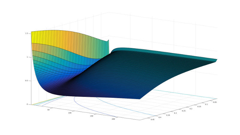
Figure 5: Energy functional $j_{n}$ with function $\varphi_{1}$ and different choices for $s$ and $\alpha$.

$$\hskip 28.45274pt\min_{s,\alpha}j_{n}(s,\alpha)$$

$$\hskip 28.45274pt\text{s.t.~{}~{}~{}}h(s,\alpha)\leq 0$$

with $h:\mathbb{R}^{2}\rightarrow\mathbb{R}^{4}$ and

$$\hskip 28.45274pth(s,\alpha)=\begin{pmatrix}-s\\ s-0.5\\ -\alpha\\ \alpha-250\end{pmatrix}.$$

Let $h_{i}$ for $i=1,2,3,4$ denote the components of the function $h$. The SQP-problem is the quadratic approximation of the associated Lagrange function

$$\hskip 28.45274ptL(s,\alpha,\lambda)=j_{n}(s,\alpha)+\sum\limits_{i=1}^{4}\lambda_{i}h_{i}(s,\alpha)$$

with

$$~{}~{}~{}~{}~{}\min_{d\in\mathbb{R}^{2}}\frac{1}{2}d^{T}\textbf{H}_{k}d+\nabla j_{n}(s_{k},\alpha_{k})^{T}d$$

$$\text{s.t~{}~{}}\nabla h_{i}(s_{k},\alpha_{k})^{T}d+h_{i}(s_{k},\alpha_{k})\leq 0~{}~{}~{}i=1,...,4.$$

The matrix $\textbf{H}_{k}$ is a positive definit approximation of the Hessian matrix from the Lagrange function $L(s,\alpha,\lambda)$. The solution $d_{k}$ of the quadratic program gives us for a suitable step size $\beta_{k}$

$$\hskip 28.45274pt\binom{s_{k+1}}{\alpha_{k+1}}=\binom{s_{k}}{\alpha_{k}}+\beta_{k}d_{k}.$$

Using the fact that

$$\hskip 28.45274pt\nabla^{2}_{s,\alpha}L(s,\alpha,\lambda)=\nabla^{2}j_{n}(s,\alpha)$$

we can argue that the approximation of the Hessian matrix $\nabla^{2}j(s,\alpha)$ is positiv definit using the argumentation structure as in the proof of Lemma 4. This implies the well-posedness of the SQP-method. For details of this algorithm we refer to the official documentation of the software library MATLAB.
For our numerical examples we obtain our noisy images $g$ from $u_{d}$, where the additve noise is normally distributed with mean zero and standard deviation $0.15$. For the obtained results, we measure the quality of reconstructions using metrics such as the peak signal-to-noise ratio (PSNR) and structural-similarity-index (SSIM). In Figures  6 and  7 we illustrate the optimal solution $\bar{u}$ of the discrete optimization problem (18) for two test images. As expected our model correlates with the standard deviation $\sigma$ as seen in Figures 9 and 8. A higher noise implies that the denoised image $\bar{u}$ has a higher deviation from the noisy image $g$ and a stronger smoothing.

(a) original image $u_{d}$

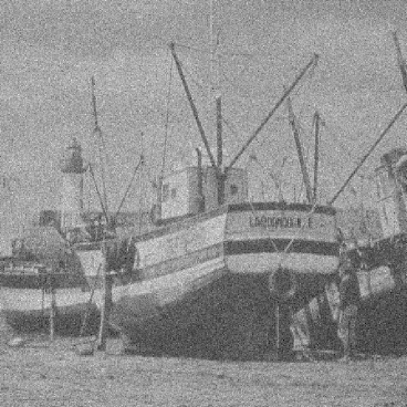
(b) image $g$;  SSIM: 0.215

(c) image $u$ with $\bar{s}=0.471,\bar{\alpha}=45.38$;  SSIM: 0.512

Figure 6: Results for the image ”boat”. As clearly seen, the model eliminates the fog based on the normally distributed noise.

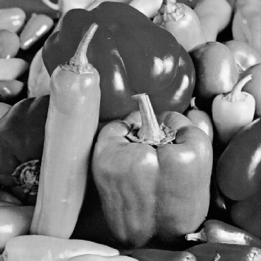
(a) original image $u_{d}$

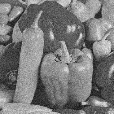
(b) noisy image $g$;  SSIM: 0.174

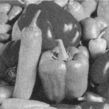
(c) image $u$ with $\bar{s}=0.475,\bar{\alpha}=48.93$; SSIM: 0.495

Figure 7: In the image ”peppers” is a significant reduction of noise while maintaining the edges.

Figure 8: We study the influence of the noise on the parameter $s$. The numerical results coincide with theoretical considerations that more noise implies a stronger smoothing of the image, i.e a higher value of the parameter $s$.

Figure 9: Also in the case of the parameter $\alpha$ the numerical results coincide with theoretical considerations. A higher noise has the result, that the denoised image is more far away from the noisy image, i.e a higher value of the parameter $\alpha$.

Furthermore, we compare our model with the ROF model RudOshFat92 , which consists in minimizing

$$\hskip 28.45274ptE(u)=\big{|}Du\big{|}_{{\mathds{T}^{d}}}+\frac{\alpha}{2}\lVert g-u\rVert^{2}.$$ (19)

for given $g\in L^{2}({\mathds{T}^{d}},\mathbb{R})$. It can be shown, that for $\alpha>0$ exists a unique minimizer $u\in BV({\mathds{T}^{d}})\cap L^{2}({\mathds{T}^{d}};\mathbb{R})$.
The minimization of the ROF model is done with a gradient flow. The variatonal derivation of total variation

$$\hskip 28.45274pt\nabla|Du\big{|}_{{\mathds{T}^{d}}}={\rm div}\,(\frac{\nabla u}{|\nabla u|}).$$

is not differentiable in $0$, so we substitute $|\nabla u(x)|$ with $\sqrt{\varepsilon^{2}+|\nabla u(x)|^{2}}$ and $\varepsilon=0.004$.
For the numerical implementation and test images we refer to Pey11 . In the ROF model we test $20$ different values for the parameter $\alpha$, all in the range of $[10^{-6},0.2]$ with equidistant distance. Afterwards we choose the parameter $\alpha$, such that we have the highest peak signal-to-noise-ratio in comparison to the reference image $u_{d}$.

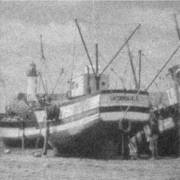
(a) Fractional-Laplacian-model; SSIM: 0.513

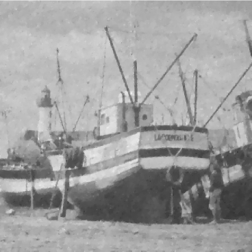
(b) ROF-model; SSIM: 0.735

Figure 10: In comparison to the fractional Laplacian model has the ROF model smoother edges. Moreover the ROF model has a better SSIM-value.

Pixels	Fractional Laplacian	Regularized ROF
128	0.38s	6.34s
256	1.23 s	22.28 s
512	5.9 s	96.26 s
1024	25.25 s	433.59 s
2048	102.1 s	2273.59 s

Figure 11: Runtime comparison between the fractional Laplacian model and the ROF model. Both model show empirically a linear runtime, but the fractional Laplacian model has a reduced computing time by factors 16-22. We used MATLAB R2015a with CPU i3-3240 and 8 GB RAM.

As in GouMor01 mentioned, the space of bounded variation $BV({\mathds{T}^{d}})$ is insufficient to describe all natural images. Therefore, we look at the image ”Baboon” as a counterexample. Figure 14 shows a part of the coat structure. A comparison between the ROF model and the Laplacian model regarding different noise levels shows that the performance of both models highly depends on the choice of the image. But we point out, that our model has a worse performance in comparison of the ROF model, as we see in Figures 12 and 13. We compare the runtime of the fractional Laplacian and the ROF model in Figure  11. Our model has a significantly lower runtime with a reduction factor of 16 to 22 in time.

Figure 12: The discrepancy of PSNR depends on the choice of the image.

Figure 13: Also for the SSIM-value the discrepancy depends on the choice of the image.

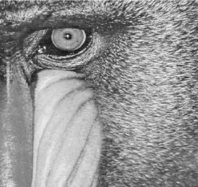
(a) original image $u_{d}$

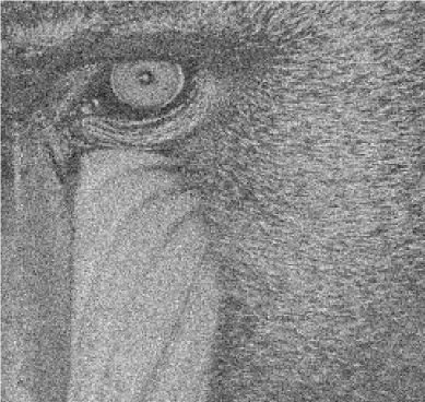
(b) noisy image $g$

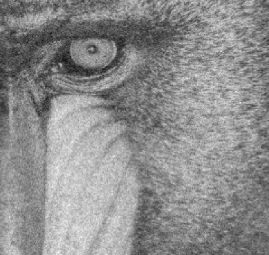
(c) Fractional-Laplacian-model; SSIM: 0.552

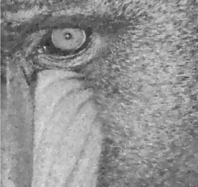
(d) ROF-model; SSIM: 0.604

Figure 14: Detail of the image ”Baboon”. The results are comparable.

6 Fractional operators in image decomposition

In the following we derive a novel approach to decompose an image using fractional differential operators. Based on the idea to decompose an image in a high and low frequency part we consider the functional

$$\hskip 14.22636ptI(u,v) =\frac{1}{2}\lVert(-\Delta)^{\frac{s_{1}}{2}}u\rVert^{2}+\frac{\alpha}{2}\lVert u+v-g\rVert^{2}+$$

$$\hskip 14.22636pt\frac{\beta}{2}\lVert R_{\frac{s_{2}}{2}}(v)\rVert^{2}$$ (20)

with $s_{1}\geq 0$ and $s_{2}\leq 0$.

6.1 Existence of a solution and solution operators

The following theorem is the main result of this section.

Theorem 6.1

For $g\in{L^{2}({\mathds{T}^{d}};\mathbb{C})}$ we define

$$~{}~{}~{}~{}~{}~{}~{}~{}~{}~{}\tilde{g}=g-\frac{1}{|{\mathds{T}^{d}}|}\int_{{\mathds{T}^{d}}}g~{}dx.$$

Then exist $\tilde{u}\in H^{s_{1}}_{0}({\mathds{T}^{d}};\mathbb{C})$ and $v\in\dot{H}^{s_{2}}({\mathds{T}^{d}};\mathbb{C})\cap{L^{2}_{0}({\mathds{T}^{d}};\mathbb{C})}$, such that the solution pair $(\tilde{u},v)$ minimizes (20). Moreover, the solutions $u:=\tilde{u}+\\ \frac{1}{|{\mathds{T}^{d}}|}\int_{{\mathds{T}^{d}}}g$ and $v$ fulfill the identity

$$~{}~{}~{}~{}~{}\int_{{\mathds{T}^{d}}}(u(x)-g(x))~{}dx=\int_{{\mathds{T}^{d}}}v(x)~{}dx=0.$$

Furthermore, the solution pair $(u,v)$ is unique.

Proof

Since $I$ is bounded from below, there exists an infimum sequence $(u_{n},v_{n})$ with

$$~{}~{}~{}~{}~{}\lVert(-\Delta)^{\frac{s_{1}}{2}}u_{n}\rVert^{2}\leq C,$$

$$~{}~{}~{}~{}~{}\lVert u_{n}+v_{n}-g\rVert^{2}\leq C,$$

$$~{}~{}~{}~{}~{}\lVert R_{\frac{s_{2}}{2}}(v_{n})\rVert^{2}\leq C.$$

The constant $C>0$ is independent of $n$.
The fact $\lVert u_{n}\rVert^{2}\leq\lVert(-\Delta)^{\frac{s_{1}}{2}}u_{n}\rVert^{2}\leq C$ yields the uniform boundedness of $u_{n}$ in ${L^{2}({\mathds{T}^{d}};\mathbb{C})}$ and therefore also the uniform boundedness of $v_{n}$ in
${L^{2}({\mathds{T}^{d}};\mathbb{C})}$. As a matter of fact, we have

$$~{}~{}~{}~{}~{}u_{n} \rightharpoonup\tilde{u}\text{ in $H^{s_{1}}_{0}({\mathds{T}^{d}};\mathbb{C})$,}$$

$$~{}~{}~{}~{}~{}v_{n} \rightharpoonup\tilde{v}\text{ in ${L^{2}({\mathds{T}^{d}};\mathbb{C})}$,}$$

$$~{}~{}~{}~{}~{}v_{n} \rightharpoonup v\text{ in $\dot{H}^{s_{2}}({\mathds{T}^{d}})$}.$$

Using the test function $w\equiv 1$ and the weak $L^{2}$-convergence, we obtain

$$\int_{{\mathds{T}^{d}}}\tilde{v}(x)~{}dx=(\tilde{v},w)=$$

$$\hskip 28.45274pt\lim\limits_{n\rightarrow\infty} (v_{n},w)=\int_{{\mathds{T}^{d}}}v_{n}(x)~{}dx=0.$$

The fact $\tilde{v}\in\dot{H}^{s_{2}}({\mathds{T}^{d}};\mathbb{C})$ allows us to identify $v$ with $\tilde{v}$. Rellich’s theorem (Theorem 2.1) implies the strong convergence of a subsequence with $u_{n}\rightarrow\tilde{u}\in{L^{2}_{0}({\mathds{T}^{d}};\mathbb{C})}$.
The weak lower semicontinuity of $I$ yields

$$\hskip 28.45274ptI(\tilde{u},v)\leq\liminf_{n\rightarrow\infty}I(u_{n},v_{n})=\inf_{w,z}I(w,z),$$

which implies the existence of a solution. To prove the uniqueness of the solution, we use the isometry property between ${L^{2}({\mathds{T}^{d}};\mathbb{C})}$ and $\ell^{2}(\mathbb{Z}^{d})$. With $\hat{g}_{0}=\hat{u}_{0}$ we obtain

$$I(\hat{\textbf{U}},\hat{\textbf{V}})=\sum\limits_{k\in\mathbb{Z}^{d}\setminus\{0\}}\frac{1}{2}|k|^{2s_{1}}|\hat{u}_{k}|^{2}$$

$$+\frac{\alpha}{2}|\hat{u}_{k}+\hat{v}_{k}-\hat{g}_{k}|^{2}+\frac{\beta}{2}|k|^{2s_{2}}|\hat{v}_{k}|^{2}.$$

Because of the uniqueness of Fourier coefficients we can differentiate for arbitrary $k\in\mathbb{Z}^{d}\setminus\{0\}$ regarding $\hat{v}_{k}$ and $\hat{u}_{k}$. In the minimum of $I(\hat{U},\hat{V})$ we get

$$\hskip 28.45274pt0 =\alpha(\hat{u}_{k}+\hat{v}_{k}-\hat{g}_{k})+\beta|k|^{2s_{2}}\hat{v}_{k},$$ (21)

$$\hskip 28.45274pt0 =|k|^{2s_{1}}\hat{u}_{k}+\alpha(\hat{u}_{k}+\hat{v}_{k}-\hat{g}_{k}).$$ (22)

for arbitrary $k\in\mathbb{Z}^{d}\setminus\{0\}$. Combining (22) and (21) imply

$$\hskip 28.45274pt\hat{u}_{k}=\frac{\beta|k|^{2s_{2}}}{|k|^{2s_{1}}}\hat{v}_{k}~{}\text{for }k\in\mathbb{Z}^{d}\setminus\{0\}.$$ (23)

Substituting (23) in (21), we obtain

$$\alpha(\frac{\beta|k|^{2s_{2}}}{|k|^{2s_{1}}}\hat{v}_{k}+\hat{v}_{k}-\hat{g}_{k})+\beta|k|^{2s_{2}}\hat{v}_{k}=0$$

$$\Leftrightarrow~{}~{}\hat{v}_{k}=\frac{\alpha\hat{g}_{k}}{\alpha\beta|k|^{2(s_{2}-s_{1})}+\alpha+\beta|k|^{2s_{2}}},$$

which implies uniquness.∎

Definition 11

Let $Y:=[s_{0},s_{3}]\times[\alpha_{0},\alpha_{1}]\times[s_{4},s_{5}]\\ \times[\beta_{0},\beta_{1}]$ with $s_{3}>s_{0}\geq 0$ and $-1\leq s_{4}<s_{5}\leq 0$. Define the solution operators $\mathcal{S}_{1},\mathcal{S}_{2}:Y\rightarrow\ell^{2}(\mathbb{Z}^{d})$ as

$$~{}~{}~{}~{}~{}~{}~{}~{}\mathcal{S}_{1}(s_{1},\alpha,s_{2},\beta)=$$

$$\hskip 22.76228pt\Bigg{[}\frac{\alpha\beta|k|^{2(s_{2}-s_{1})}\hat{g}_{k}}{\alpha\beta|k|^{2(s_{2}-s_{1})}+\alpha+\beta|k|^{2s_{2}}}\Bigg{]}_{k\in\mathbb{Z}^{d}\setminus\{0\}}$$ (24)

and

$$~{}~{}~{}~{}~{}~{}~{}~{}\mathcal{S}_{2}(s_{1},\alpha,s_{2},\beta)=$$

$$\hskip 22.76228pt\Biggl{[}\frac{\alpha\hat{g}_{k}}{\alpha\beta|k|^{2(s_{2}-s_{1})}+\alpha+\beta|k|^{2s_{2}}}\Biggl{]}_{k\in\mathbb{Z}^{d}\setminus\{0\}}.$$ (25)

6.2 Relation to other image models

In the following we study the behavior in the limiting case when the regularization parameters $\alpha$ and $\beta$ tend to infinity.

Lemma 6

Let $\beta>0$ be and $g\in{L^{2}_{0}({\mathds{T}^{d}};\mathbb{C})}$. With $\alpha_{n}$ we denote an increasing, positive sequence, such that $\lim\limits_{n\rightarrow}\alpha_{n}=\infty$. The pair $(u_{\alpha_{n}},v_{\alpha_{n}})$ is the unique minimum (20) for the specific $\alpha_{n}$.
The sequence $(u_{\alpha_{n}},v_{\alpha_{n}})$ is bounded and a subsequence converges weakly to $(u_{0},g-u_{0})$, with $u_{0}$ is the unique minimizer of

$$\hskip 5.69046ptI(u):=\frac{1}{2}\lVert(-\Delta)^{\frac{s_{1}}{2}}u\rVert^{2}+\frac{\beta}{2}\lVert R_{\frac{s_{2}}{2}}(u-g)\rVert^{2}.$$ (26)

Proof

The proof follows AujGilChaOsh05 . The existence of a solution $(u_{\alpha_{n}},v_{\alpha_{n}})$ for the specific $\alpha_{n}$ follows from (6.1). Moreover, we have

$$\hskip 28.45274ptI(u_{\alpha_{n}},v_{\alpha_{n}})\leq I(0,g)=\frac{\beta}{2}\lVert R_{\frac{s_{2}}{2}}(g)\rVert^{2},$$

which implies the boundedness of the sequence
$(u_{\alpha_{n}},v_{\alpha_{n}})$ independent of $n\in\mathbb{N}$. Furthermore, this implies the weak convergence of a subsequence to $u_{0}$ in $H^{s_{1}}_{0}({\mathds{T}^{d}};\mathbb{C})$ respectivly $v_{0}$ in $\dot{H}^{s_{2}}({\mathds{T}^{d}};\mathbb{C})\cap{L^{2}_{0}({\mathds{T}^{d}};\mathbb{C})}$. The estimate

$$\lVert u_{n}+v_{n}-g\rVert^{2}\leq\frac{\beta}{2\alpha_{n}}\lVert R_{\frac{s_{2}}{2}}(g)\rVert^{2}$$

for all $n\in\mathbb{N}$ guarantees

$$\hskip 28.45274pt\lVert u_{0}+v_{0}-g\rVert^{2} =0,$$

$$\hskip 28.45274ptu_{0}(x)+v_{0}(x) =g(x)~{}~{}\text{a. e.}$$

in the limiting case $n\rightarrow\infty$. For arbitrary $u\in H^{s_{1}}_{0}({\mathds{T}^{d}};\mathbb{C})$ we have

$$\frac{1}{2}\lVert(-\Delta)^{\frac{s_{1}}{2}}u\rVert^{2}+\frac{\alpha_{n}}{2}\lVert u+(g-u)-g\rVert^{2}$$

$$+\frac{\beta}{2}\lVert R_{\frac{s_{2}}{2}}(u-g)\rVert^{2}$$

$$\geq\frac{1}{2}\lVert(-\Delta)^{\frac{s_{1}}{2}}u_{\alpha_{n}}\rVert^{2}+\frac{\alpha_{n}}{2}\lVert u_{\alpha_{n}}+v_{\alpha_{n}}-g\rVert^{2}$$

$$+\frac{\beta}{2}\lVert R_{\frac{s_{2}}{2}}(v_{\alpha_{n}})\rVert^{2}$$

$$\geq\frac{1}{2}\lVert(-\Delta)^{\frac{s_{1}}{2}}u_{\alpha_{n}}\rVert^{2}+\frac{\beta}{2}\lVert R_{\frac{s_{2}}{2}}(v_{\alpha_{n}})\rVert^{2}$$

for all $n\in\mathbb{N}$. The weak lower semicontinuity of the functional yields

$$\hskip 28.45274pt\frac{1}{2}\lVert(-\Delta)^{\frac{s_{1}}{2}}u_{0}\rVert^{2}+\frac{\beta}{2}\lVert R_{\frac{s_{2}}{2}}(g-u_{0})\rVert^{2}$$

$$\leq\liminf_{n\rightarrow\infty}\frac{1}{2}\lVert(-\Delta)^{\frac{s_{1}}{2}}u_{\alpha_{n}}\rVert^{2}+\frac{\beta}{2}\lVert R_{\frac{s_{2}}{2}}(v_{\alpha_{n}})\rVert^{2}.$$

From this we conclude that $(u_{0},g-u_{0})$ is the unique minimizer of (26).∎

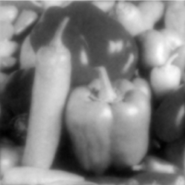
(a) $u$ with $\alpha=0.001$

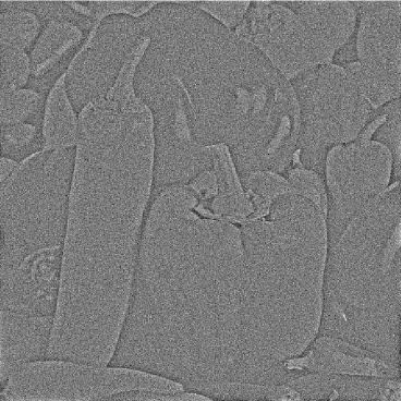
(b) $v$ with $\alpha=0.001$

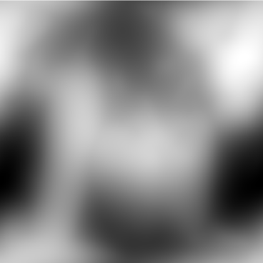
(c) $u$ with $\alpha=1000$

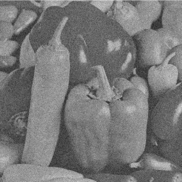
(d) $v$ with $\alpha=1000$

Figure 15: Image components with fixed $s_{1}=0.2,s_{2}=-1,\beta=1$ and different choices for parameter $\alpha$ for the noise-free image. The choice of the parameter $\alpha$ has a strong impact on the decomposition.

We can prove a similiar result in the limiting case when $\beta$ tends to infinity.

Lemma 7

Let $g\in{L^{2}({\mathds{T}^{d}};\mathbb{C})}$ be and $\alpha>0$. With $\beta_{n}$ we denote an increasing, positive sequence, such that $\lim\limits_{n\rightarrow}\beta_{n}=\infty$. The pair is the unique minimum $(u_{\beta_{n}},v_{\beta_{n}})$ for this specific $\beta_{n}$. The sequence $(u_{\beta_{n}},v_{\beta_{n}})$ is bounded and a subsequence converges weakly to $(u_{0},0)$, with $u_{0}$ is minimizer of (3).

Proof

Without loss of generality we assume, that $\int_{{\mathds{T}^{d}}}g(x)~{}dx=0$. The existence of a solution
$(u_{\beta_{n}},v_{\beta_{n}})$ follows directly from (6.1). This yields

$$\hskip 28.45274ptI(u_{\beta_{n}},v_{\beta_{n}})\leq I(0,0)=\frac{\alpha}{2}\lVert g\rVert^{2}$$

for all $n\in\mathbb{N}$. As a consequence we have the boundedness of the sequence $(u_{\beta_{n}},v_{\beta_{n}})$, which implies the existence of weakly convergent subsequences to $u_{0}$ in $H^{s_{1}}_{0}({\mathds{T}^{d}};\mathbb{C})$ respectively $v_{0}$ in $\dot{H}^{s_{2}}({\mathds{T}^{d}};\mathbb{C})\cap{L^{2}_{0}({\mathds{T}^{d}};\mathbb{C})}$. We obtain

$$\hskip 28.45274pt\lVert R_{\frac{s_{2}}{2}}(v_{\beta_{n}})\rVert^{2}\leq\frac{\alpha}{2\beta_{n}}\lVert g\rVert^{2}=I(0,0)~{}\rightarrow 0$$

for $n\rightarrow\infty$ and therefore

$$\hskip 28.45274ptv_{\beta_{n}}\rightarrow 0=v~{}~{}\text{in~{}}\dot{H}^{s_{2}}({\mathds{T}^{d}};\mathbb{C}),$$

i.e. $\lim\limits_{n\rightarrow\infty}\sum\limits_{k\in\mathbb{Z}^{d}\setminus\{0\}}|k|^{2s_{2}}|\hat{v}_{\beta_{n},k}|^{2}=0$.
To prove the weak convergence of $v_{\beta_{n}}$ to 0 in
${L^{2}_{0}({\mathds{T}^{d}};\mathbb{C})}$, we choose an arbitrary function $w\in{L^{2}_{0}({\mathds{T}^{d}};\mathbb{C})}$.
The function $R_{s_{2}}(w)=\frac{1}{(2\pi)^{d}}\sum\limits_{k\in\mathbb{Z}^{d}\setminus\{0\}}|k|^{2s_{2}}\hat{w}_{k}\varphi^{k}$ as an element in ${L^{2}_{0}({\mathds{T}^{d}};\mathbb{C})}$ is well-defined and we obtain in the limiting case $n\rightarrow\infty$

$$\hskip 14.22636pt(v_{0},R_{s_{2}}(w))_{{L^{2}_{0}({\mathds{T}^{d}};\mathbb{C})}}\leftarrow(v_{\beta_{n}},R_{s_{2}}(w))_{{L^{2}_{0}({\mathds{T}^{d}};\mathbb{C})}}$$

$$\hskip 28.45274pt=\frac{1}{(2\pi)^{d}}\sum\limits_{k\in\mathbb{Z}^{d}\setminus\{0\}}|k|^{2s_{2}}\hat{v}_{\beta_{n},k}\overline{\hat{w}_{k}}$$

$$\hskip 28.45274pt=\frac{1}{(2\pi)^{d}}(v_{\beta_{n}},w)_{\dot{H}^{s_{2}}({\mathds{T}^{d}};\mathbb{C})}\rightarrow 0$$

and therefore $v_{0}\rightharpoonup 0$ in ${L^{2}_{0}({\mathds{T}^{d}};\mathbb{C})}$.
Using the minimizer property of the sequence
$(u_{\beta_{n}},v_{\beta_{n}})$ we have for arbitrary $u\in H^{s_{1}}_{0}({\mathds{T}^{d}};\mathbb{C})$

$$\frac{1}{2}\lVert(-\Delta)^{\frac{s_{1}}{2}}u\rVert^{2}+\frac{\alpha}{2}\lVert u-g\rVert^{2}=\frac{1}{2}\lVert(-\Delta)^{\frac{s_{1}}{2}}u\rVert^{2}$$

$$\hskip 28.45274pt+\frac{\alpha}{2}\lVert u+0-g\rVert^{2}+\frac{\beta_{n}}{2}\lVert R_{\frac{s_{2}}{2}}(0)\rVert^{2}$$

$$\hskip 28.45274pt\geq\frac{1}{2}\lVert(-\Delta)^{\frac{s_{1}}{2}}u_{\beta_{n}}\rVert^{2}+\frac{\alpha}{2}\lVert u_{\beta_{n}}+v_{\beta_{n}}-g\rVert^{2}$$

$$\hskip 28.45274pt+\frac{\beta_{n}}{2}\lVert R_{\frac{s_{2}}{2}}(v_{\beta_{n}})\rVert^{2}$$

for all $n\in\mathbb{N}$.
Because of the weak lower semicontinuity we get

$$\hskip 28.45274pt\frac{1}{2}\lVert(-\Delta)^{\frac{s_{1}}{2}}u_{0}\rVert^{2}+\frac{\alpha}{2}\lVert u_{0}-g\rVert^{2}$$

$$\leq\liminf_{n\rightarrow\infty}\frac{1}{2}\lVert(-\Delta)^{\frac{s_{1}}{2}}u_{\beta_{n}}\rVert^{2}+\frac{\alpha}{2}\lVert u_{\beta_{n}}+v_{\beta_{n}}-g\rVert^{2}$$

$$\hskip 28.45274pt+\frac{\beta_{n}}{2}\lVert R_{\frac{s_{2}}{2}}(v_{\beta_{n}})\rVert^{2}.$$

This shows that $u_{0}$ is minimizer of (3).∎

7 Image decomposition and numerical experiments

We first show an error estimate between the continous and discrete solution for fixed, but arbitrary parameters.

Lemma 8

Let $s_{1},\alpha,s_{2},\beta$ be fixed, but arbitrarily chosen. The associated pair $(\textbf{u}=\mathcal{S}_{1}(s_{1},\alpha,s_{2},\beta),\\ \textbf{v}=\mathcal{S}_{2}(s_{1},\alpha,s_{2},\beta)$ is a minimizer of (20). The pair $(\textbf{u}_{n}=\mathcal{S}_{1,n}(s_{1},\alpha,s_{2},\beta),\textbf{v}_{n}=\mathcal{S}_{2,n}(s_{1},\alpha,s_{2},\beta))$ is the solution of the associated discrete problem in the trigonometric space $\mathcal{T}_{n}$.
Then we obtain the error estimate

$$\hskip 14.22636pt|\textbf{u}-\textbf{u}_{n}|^{2}_{s_{1}}+\beta|\textbf{v}_{n}-\textbf{v}|^{2}_{s_{2}}+\frac{\alpha}{2}\lVert\textbf{u}_{n}+\textbf{v}_{n}-\textbf{u}-\textbf{v}\rVert_{\ell^{2}}^{2}$$

$$\hskip 14.22636pt\leq\frac{\alpha}{2}\lVert\widehat{\textbf{G}}-\widehat{\textbf{G}}_{n}\rVert_{\ell^{2}}^{2}.$$

Proof

The solution pair $(\textbf{u},\textbf{v})$ fulfills the Euler-Lagrange equation

$$(-\Delta)^{s_{1}}\textbf{u}+\alpha(\textbf{u}+\textbf{v}-\widehat{\textbf{G}})=0\text{ in $\ell^{2}(\mathbb{Z}^{d})$}$$

and

$$\alpha(\textbf{u}+\textbf{v}-\widehat{\textbf{G}})+\beta R_{s_{2}}(\textbf{v})=0\text{ in $\ell^{2}(\mathbb{Z}^{d})$}.$$

We obtain an analogous Euler-Lagrange equation for the solution pair $(\textbf{u}_{n},\textbf{v}_{n})$. We have

$$\hskip 28.45274pt|\textbf{u}-\textbf{u}_{n}|_{s_{1}}=$$

$$\hskip 28.45274pt-\alpha(\textbf{u}_{n}+\textbf{v}_{n}-\hat{\textbf{g}}_{n}-\textbf{u}-\textbf{v}+\widehat{\textbf{G}},\textbf{u}_{n}-\textbf{u})_{\ell^{2}}$$

and

$$\hskip 28.45274pt\beta|\textbf{v}_{n}-\textbf{v}|_{s_{2}}=$$

$$\hskip 28.45274pt-\alpha(\textbf{u}_{n}+\textbf{v}_{n}-\widehat{\textbf{G}}_{n}-\textbf{u}-\textbf{v}+\widehat{\textbf{G}},\textbf{v}_{n}-\textbf{v})_{\ell^{2}}.$$

Using the Cauchy-Schwarz and Young
inequality yields

$$|\textbf{u}-\textbf{u}_{n}|_{s_{1}}+\beta|\textbf{v}_{n}-\textbf{v}|_{s_{2}}=$$

$$\alpha(-\textbf{u}_{n}-\textbf{v}_{n}+\widehat{\textbf{G}}_{n}+\textbf{u}+\textbf{v}-\widehat{\textbf{G}},\textbf{u}_{n}+\textbf{v}_{n}-\textbf{u}-\textbf{v})_{\ell^{2}}$$

$$=-\alpha\lVert\textbf{u}_{n}+\textbf{v}_{n}-\textbf{u}-\textbf{v}\rVert^{2}_{\ell^{2}}+$$

$$~{}~{}~{}~{}\alpha(\widehat{\textbf{G}}_{n}-\widehat{\textbf{G}},\textbf{u}_{n}+\textbf{v}_{n}-\textbf{u}-\textbf{v})_{\ell^{2}}$$

$$\leq\frac{-\alpha}{2}\lVert\textbf{u}_{n}+\textbf{v}_{n}-\textbf{u}-\textbf{v}\rVert^{2}_{\ell^{2}}+\frac{\alpha}{2}\lVert\widehat{\textbf{G}}-\widehat{\textbf{G}}_{n}\rVert^{2}_{\ell^{2}}.$$

This implies the assertion.∎

7.1 Numerical experiments

For the numerical experiments we consider the optimization problem

$$j_{n}(s_{1},\alpha,s_{2},\beta)=\frac{1}{2}\lVert\mathcal{S}_{1,n}(s_{1},\alpha,s_{2},\beta)-\hat{\textbf{U}}^{n}_{d}\rVert^{2}_{l^{2}}$$

$$\hskip 28.45274pt+\varphi(s_{1},\alpha,s_{2},\beta)$$ (27)

$$\hskip 28.45274pt\text{s.t. }(s_{1},\alpha,s_{2},\beta)\in W.$$

with the discrete solution operator $\mathcal{S}_{1,n}$. For the convex set $W$ we choose

$$\hskip 28.45274pt[0,0.5]\times[0.01,10^{4}]\times[-1,0]\times[0,10^{5}]$$

and as the strong convex function $\varphi$

$$\hskip 28.45274pt\varphi(s_{1},\alpha,s_{2},\beta)=$$

$$\hskip 28.45274pt\frac{1}{s_{1}(0.5-s_{1})}+\frac{1}{(\alpha-0.01)(10^{4}-\alpha)}$$

$$\hskip 28.45274pt+\frac{1}{-s_{2}(s_{2}+1)}+\frac{1}{\beta(10^{5}-\beta)}.$$

The scaling factor of the function $\varphi$ is $3\cdot 10^{-7}$.
The noise is normal distributed with mean value $\mu=0$ and standard deviation $\sigma=0.15$. In all numerical experiments we see a better reconstruction of the original image in comparison to the fractional model (18), see for example Figure 16.

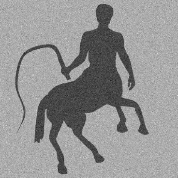
(a) noisy image $g$
 

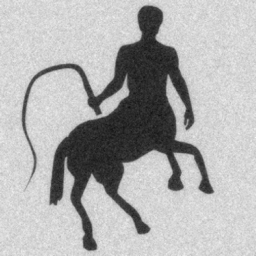
(b) Fractional-Laplacian model (18); SSIM: 0.356

(c) component $u$ of (27); SSIM: 0.581

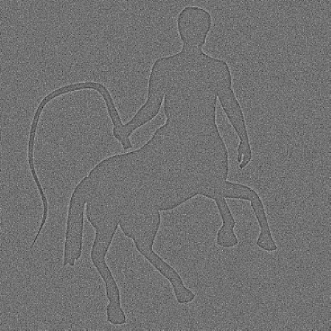
(d) component $v$ of (27)

Figure 16: Decompositon of the image ”kentaur” with optimal parameters $\bar{s_{1}}=0.172,~{}\bar{\alpha}=9999.7,~{}\bar{s_{2}}=-0.926$ and $\bar{\beta}=10410$. We see a significantly improvement of the SSIM-value.

7.2 Comparison with OSV model

To compare our model we choose a modification of the ROF model, as shown in OshSolVes03 .
There the $L^{2}$-norm is replaced by the weaker $H^{-1}$-norm, such that finer details are better
reconstructed. Therefore, we assume that $g-u=\operatorname{div}(\vec{v})$ with $\vec{v}\in{L^{2}({\mathds{T}^{d}};\mathbb{C})}^{2}$. This yields a unique hodge-decomposition

$$\hskip 28.45274ptv=\nabla P+\vec{Q}$$

with $P\in H^{1}({\mathds{T}^{d}})$ and a divergence-free vector field $\vec{Q}$. Using $g-u=\operatorname{div}(\vec{v})=\Delta P$ we have $P=\Delta^{-1}(g-u)$. Combining all arguments has as result the convex minimization problem

$$\inf_{u}E(u)=\int_{{\mathds{T}^{d}}}|\nabla u|+\alpha\int_{{\mathds{T}^{d}}}|\nabla(\Delta^{-1}(g-u))|^{2}.$$ (28)

which has a solution.
For the numerical implementation we refer to Pey11 . In Figure 17 and 18 we compare the Riesz model (27) and the OSV model (28). The Riesz model can separate the textural component $v$ much better than the OSV model.

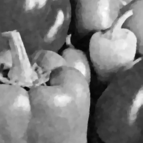
(a) component $u$ of (28); SSIM: 0.798

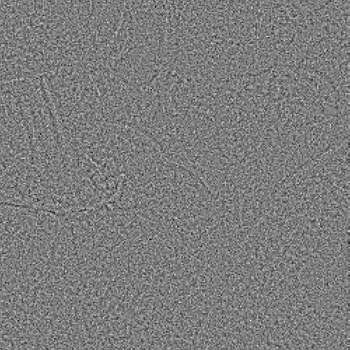
(b) component $g-u$ of (28)

(c) component $u$ of (27); SSIM: 0.716

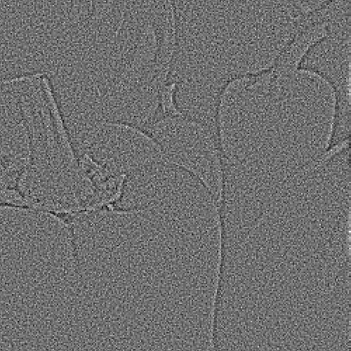
(d) component $v$ of (27)

Figure 17: Detail of the image ”pepper” ($\sigma=0.1$). The model (28) can not sufficiently distinguish between noise and component $v$.

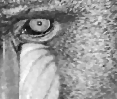
(a) component $u$ of (28); SSIM: 0.553

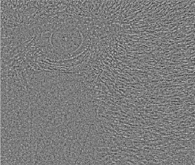
(b) component $g-u$ of (28)

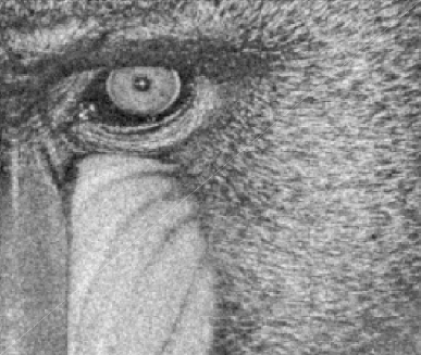
(c) component $u$ of (27); SSIM: 0.691

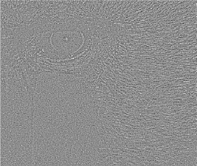
(d) component $v$ of (27)

Figure 18: Detail of the image ”Baboon” ($\sigma=0.1$).

8 Conclusion and outlook

In this work we illustrated the possibilities of fractional differential operators in image regularization and decomposition. Working with the Fourier transform we can easily define solution operators. In the case of image regularization the analysis of the solution operator $\mathcal{S}$ allows us to define and analyse a bilevel optimization problem to determine the optimal values for the parameter $s$ and $\alpha$. In contrast to Deep Learning approaches we obtain error estimates and are able to derive an analytical understanding of the problem. The theoretical considerations correlate with the numerical experiments. As an advantage in comparison to the ROF model we can automatically determine the optimal parameters, but we have slightly worse SSIM-values. We point out, that our model has a lower runtime. An open question for further investigations is the choice of a suitable metric to compare the denoised image $u$ and the original image $u_{d}$. The $L^{2}$-norm only considers the absolut difference between two images and no structural similarity between them. In the case of image decomposition we introduced a new functional. We proved existence and uniqueness of the solution regarding this model. Moreover, our model can approximate other image decompositon models in the limiting case when $\alpha$ or $\beta$ tends to infinity. The numerical experiments show better results than the fractional Laplacian model. The comparison with the OSV model yields comparable results. Furthermore, we point out, that our model can reconstruct the image component $v$ better than the OSV model. The extension to color images is a point of future research. An experimental setup in case of fractional image denoising indicates that the use of quaternionic Fourier transform seems to be the right choice.

References

• (1) Antil, H., Bartels, S.: Spectral approximation of fractional PDEs in image processing and phase field modeling. Comput. Methods Appl. Math. 17(4), 661–678 (2017). DOI 10.1515/cmam-2017-0039. URL https://doi.org/10.1515/cmam-2017-0039
• (2) Antil, H., Khatri, R., et al.: Bilevel optimization, deep learning and fractional laplacian regularization with applications in tomography. arXiv preprint arXiv:1907.09605 (2019)
• (3) Antil, H., Otárola, E., Salgado, A.J.: Optimization with respect to order in a fractional diffusion model: analysis, approximation and algorithmic aspects. J. Sci. Comput. 77(1), 204–224 (2018). DOI 10.1007/s10915-018-0703-0. URL https://doi.org/10.1007/s10915-018-0703-0
• (4) Antil, H., Rautenberg, C.N.: Sobolev spaces with non-Muckenhoupt weights, fractional elliptic operators, and applications. SIAM J. Math. Anal. 51(3), 2479–2503 (2019). DOI 10.1137/18M1224970. URL https://doi.org/10.1137/18M1224970
• (5) Aujol, J.F., Gilboa, G., Chan, T., Osher, S.: Structure-texture image decomposition—modeling, algorithms, and parameter selection. International Journal of Computer Vision 67(1), 111–136 (2006). DOI 10.1007/s11263-006-4331-z. URL https://doi.org/10.1007/s11263-006-4331-z
• (6) Boyd, S., Vandenberghe, L.: Convex optimization. Cambridge University Press, Cambridge (2004). DOI 10.1017/CBO9780511804441. URL https://doi.org/10.1017/CBO9780511804441
• (7) Boyer, F., Fabrie, P.: Mathematical tools for the study of the incompressible Navier-Stokes equations and related models, Applied Mathematical Sciences, vol. 183. Springer, New York (2013). DOI 10.1007/978-1-4614-5975-0. URL https://doi.org/10.1007/978-1-4614-5975-0
• (8) Bueno-Orovio, A., Kay, D., Burrage, K.: Fourier spectral methods for fractional-in-space reaction-diffusion equations. BIT 54(4), 937–954 (2014). DOI 10.1007/s10543-014-0484-2. URL https://doi.org/10.1007/s10543-014-0484-2
• (9) Gousseau, Y., Morel, J.M.: Are natural images of bounded variation? SIAM J. Math. Anal. 33(3), 634–648 (2001). DOI 10.1137/S0036141000371150. URL https://doi.org/10.1137/S0036141000371150
• (10) Liu, P., Schönlieb, C.B.: Learning optimal orders of the underlying euclidean norm in total variation image denoising. arXiv preprint arXiv:1903.11953 (2019)
• (11) Liu, Q., Zhang, Z., Guo, Z.: On a fractional reaction-diffusion system applied to image decomposition and restoration. Comput. Math. Appl. 78(5), 1739–1751 (2019). DOI 10.1016/j.camwa.2019.05.030. URL https://doi.org/10.1016/j.camwa.2019.05.030
• (12) Nesterov, Y.: Introductory Lectures on Convex Optimization. Springer US (2004). DOI 10.1007/978-1-4419-8853-9. URL https://doi.org/10.1007/978-1-4419-8853-9
• (13) Osher, S., Solé, A., Vese, L.: Image decomposition and restoration using total variation minimization and the $H^{-1}$ norm. Multiscale Model. Simul. 1(3), 349–370 (2003). DOI 10.1137/S1540345902416247. URL https://doi.org/10.1137/S1540345902416247
• (14) Peyré, G.: The numerical tours of signal processing. Computing in Science & Engineering 13(4), 94–97 (2011). DOI 10.1109/mcse.2011.71. URL https://doi.org/10.1109/mcse.2011.71
• (15) Rudin, L.I., Osher, S., Fatemi, E.: Nonlinear total variation based noise removal algorithms. Phys. D 60(1-4), 259–268 (1992). DOI 10.1016/0167-2789(92)90242-F. URL https://doi.org/10.1016/0167-2789(92)90242-F. Experimental mathematics: computational issues in nonlinear science (Los Alamos, NM, 1991)
• (16) Saranen, J., Vainikko, G.: Periodic integral and pseudodifferential equations with numerical approximation. Springer Monographs in Mathematics. Springer-Verlag, Berlin (2002). DOI 10.1007/978-3-662-04796-5. URL https://doi.org/10.1007/978-3-662-04796-5
• (17) Sprekels, J., Valdinoci, E.: A new type of identification problems: optimizing the fractional order in a nonlocal evolution equation. SIAM J. Control Optim. 55(1), 70–93 (2017). DOI 10.1137/16M105575X. URL https://doi.org/10.1137/16M105575X