Standing autoresonant plasma waves

Abstract

Formation and control of strongly nonlinear standing plasma waves (SPWs) from a trivial equilibrium by a chirped frequency drive is discussed. If the drive amplitude exceeds a threshold, after passage through the linear resonance in this system, the excited wave preserves the phase-locking with the drive yielding a controlled growth of the wave amplitude. We illustrate these autoresonant waves via Vlasov-Poisson simulations showing formation of sharply peaked excitations with local electron density maxima significantly exceeding the unperturbed plasma density. The Whitham’s averaged variational approach applied to a simplified water bag model yields the weakly nonlinear evolution of the autoresonant SPWs and the autoresonance threshold. If the chirped driving frequency approaches some constant level, the driven SPW saturates at a target amplitude avoiding the kinetic wave breaking.

1 Introduction

Plasmas can sustain laser intensities many orders of magnitude larger than typical solid state optical components. This makes plasmas attractive for manipulation and control of intense laser beams, but requires formation of large and stable electron density structures in the plasma to impact the propagation of the laser light significantly. A typical approach to this problem is via ponderomotive forces using additional driving laser beams. Several applications of plasma photonics based on light scattering off electron density structures have been proposed including short pulse amplification via the resonant excitation of plasma waves (Malkin et al., 1999), transient plasma gratings (Lehmann & Spatachek, 2016), crossed-beam energy transfer for symmetry control in ICF (Michel et al., 2009), and, more recently, plasma-based polarization control (Michel et al., 2014; Turnbull et al., 2016, 2017; Lehmann & Spatschek, 2018). The efficiency is an important factor in all these applications, as the goal is to create the largest amplitude plasma density perturbation using smallest possible driver intensities. Recently, it was shown that very large amplitude travelling or standing ion acoustic waves (SIAW) can be excited via the autoresonance (AR) approach (Friedland & Shagalov, 2014, 2017; Friedland et al., 2019). The latter exploits the salient property of nonlinear waves to stay in resonance with driving perturbations if some parameter in the system (e.g., the driving frequency) varies in time [for a review of several AR applications see (Fajans & Friedland, 2001; Friedland, 2009)]. Such systems preserve the resonance with the drive via self-adjustment of the driven wave amplitude leading to a large amplitude amplification even when the driver is relatively weak. In this paper, we will discuss the AR approach to excitation of very large amplitude standing plasma waves (SPW) using both the kinetic and a simplified water bag models. The nonlinear SIAWs (Friedland et al., 2019) and SPWs [see a related analysis of nonlinear Trivelpiece-Gould waves (Dubin & Ashourvan, 2015)] are much more complex than their traveling wave counterparts. For example, the autoresonant SIAW driven to large amplitudes by a weak, chirped frequency standing ponderomotive wave is a two-phase solution, each phase locked to one of the traveling waves comprising the drive (Friedland et al., 2019). The peak electron density in these waves can reach several times the initial plasma density. We will show that similar giant plasma structures can be excited in the form of autoresonant SPWs.

The paper is organized as follows. In Sec. 2, we will illustrate autoresonant SPWs in Vlasov-Poisson simulations and compare the results to those from the a simplified water bag model presented in Sec. 3. We will discuss weakly nonlinear SPWs in Sec. 4 and use their form as an ansatz in developing a weakly nonlinear theory of driven-chirped SPWs based on the Whitham’s averaged variational principle (Whitham, 1974) in Sec. 5. In Sec. 6, we reduce a system of slow coupled amplitude-phase mismatch equations yielding the autoresonance threshold on the driving amplitude for excitation of autoresonant SPWs. In the same section, we will also discuss the control of large amplitude autoresonant SPW by tailoring the time dependence of the driving frequency. Finally, Sec. 7 will present our conclusions.

2 Standing autoresonant plasma waves in Vlasov-Poison simulations

Our study of autoresonant SPWs is motivated by numerical simulations of the following one-dimensional Vlasov-Poisson (VP) system describing an externally driven plasma wave

$$f_{t}+uf_{x}+(\varphi+\varphi_{d})_{x}f_{u}=0,\varphi_{xx}=\kappa^{2}\varphi+\int fdu-1.$$ (1)

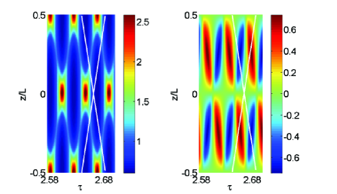
Figure 1: (color online) The colormap of the waveforms of the electron density $n$ (left panel) and fluid velocity $v$ (right panel) in the final time interval $\delta\tau=0.125$ of the simulation. The slopes of the white lines are the phase velocities of the two traveling waves comprising the drive.

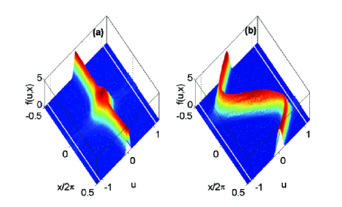
Figure 2: (color online) The snapshots of the electron distribution function at two times $\tau=2.69$ [panel (a)] and $2.7$ [panel (b)] during the last period of the wave oscillation in Fig. 1. The fluid velocity vanishes in panel (a), while the electron density reaches its maximal value of $2.5$. In contrast, in panel (b), the fluid velocity $|v|$ is at its maximum at two locations in $x$. The straight white lines are at the locations of the phase velocities $\pm\omega_{d}/k$

Here we assume constant ion density, $f$ and $\varphi$ are the electron velocity distribution and the electric potential, and $\varphi_{d}=2\varepsilon\cos(kx)\cos\theta_{d}$, where $\theta_{d}=kx-\int\omega_{d}dt$ is a small amplitude standing wave-like ponderomotive potential having a slowly varying frequency $\omega_{d}(t)$. All dependent and independent variables in (1) are dimensionless, such that the position, time, and velocity are rescaled with respect to $1/k$, the inverse plasma frequency $\omega_{p}^{-1}=\sqrt{m/(4\pi e^{2}n_{0})}$ ($n_{0}$ being the ion density), and $\omega_{p}/k$. Then, in the dimensionless form of the driving phase, $k=1$ and $\omega_{d}$ is rescaled by $\omega_{p}$. The distribution function and the potentials in (1) are rescaled with respect to $kn_{0}/\omega_{p}$, and $m\omega_{p}^{2}/(ek^{2})$, respectively. We have also added an effective screening term $\kappa^{2}\varphi$ in Poisson equation modeling the typical finite radial extent of the ponderomotive potential (Dubin & Ashourvan, 2015). We assume $2\pi$ periodicity in $x$ and solve the time evolution problem, subject to simple initial equilibrium $\varphi(x,0)=0$ and $f(u,x,0)=(2\pi\sigma^{2})^{-1/2}\exp(-u^{2}/2\sigma^{2})$, where $\sigma=k\lambda_{D}$ ($\lambda_{D}=u_{e}/\omega_{p}$ being the Debye length and $u_{e}$ the initial electron thermal velocity). Note that $\sigma$, $\kappa$ and the driving parameters fully define our rescaled, dimensionless problem. Finally, we are interested in the driving frequency of the order of the plasma frequency and, consequently, assume $\sigma\ll 1$ to avoid the kinetic Landau resonance ($\omega_{d}/k\approx u$) initially.

We have applied our VP code (Friedland et al., 2006) for solving this problem numerically and show some results of the simulations in Figs. 1-4 for $\sigma=0.1$, $\kappa=0$ (the effect of the nonzero $\kappa$ will be discussed later), and driving frequency (dimensionless) $\omega_{d}=\omega_{0}+\alpha t$, where $\omega_{0}=\sqrt{(1+\kappa^{2})^{-1}+3\sigma^{2}}$ is the normalized plasma wave frequency in the linearized warm fluid model [see Eq. (9)], while $\alpha=0.00005$ and $\varepsilon=0.0021$. We present the results of the simulations versus slow time $\tau=\alpha^{1/2}t$ (a convenient representation in AR problems), as the system evolves between initial $\tau_{0}=-5$ and final $\tau_{1}=2.7$ times (the total dimensionless time in this simulation is $\Delta t=7.7/\alpha^{1/2}=1089$, i.e., $173$ periods of plasma oscillations). Figure 1 shows the waveform of the electron density $n=\int fdu$ and fluid velocity $v=\int ufdu$ in a small time window $\delta\tau=0.125\,$ of the evolution just before reaching $\tau_{1}$. One can see a very large amplitude SPW with its peak electron density reaching $2.5$ times the initial plasma density (unity in our dimensionless problem). Furthermore, as expected, for a given time, the solutions are $2\pi$ periodic in $x$. But there also exist two directions shown by white lines in the figure with slopes $dx/d\tau=\pm\omega_{d}/\alpha^{1/2}$ (these slopes are the phase velocities of the two traveling waves comprising the drive) along which the solutions are $\pi$ periodic. This suggests that $u,n$ are periodic functions of  three arguments $\Theta_{1},\Theta_{2},x$, where $\Theta_{1,2}=x\pm\int\omega_{d}t$ and the solutions are $2\pi$ periodic in $\Theta_{1,2}$ and $\pi$ periodic in $x.$ Similar two-phase solutions, with each phase $\Theta_{1,2}$ locked to one of the phases of the waves comprising the drive were also observed in autoresonant SIAWs (Friedland et al., 2019). The occurrence of multi-phase solutions is known in the theory of some partial differential equations (Novikov et al., 1984).

Additional results of the simulations are presented in Fig. 2, showing the snapshots of the electron distribution function at two different times inside $\delta\tau$. Figure 2a corresponds to the time when the fluid velocity vanishes, while the electron density reaches its maximal value of $2.5$, while at the time in Fig. 2b the fluid velocity $|v|$ is at its maximum at two locations in $x$. The white horizontal lines in Fig. 2 show the locations of the phase velocities $\pm\omega_{d}/k$ associated with the traveling waves comprising the drive. One can see in Fig. 2b that a small fraction of the electrons in the tail of the distribution reaches the Landau resonance, indicating proximity to the kinetic wave breaking.

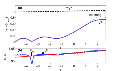
Figure 3: (color online) The excitation of the autoresonant SPW for driving amplitude above the AR threshold. Panel (a): the envelope of the maxima of the electron fluid velocity $v$ versus slow time $\tau=\alpha^{1/2}t$ in VP simulations (blue solid line) are compared to water bag model simulations (dotted red line). The dashed line represents the phase velocity $\omega_{d}/k$ of the driving wave. Panel (b) shows the frequencies of the driving (straight line) and driven (dotted line) waves. The continuous AR frequency locking is seen starting $\tau\approx-3$.

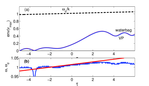
Figure 4: (color online) The numerical simulations as in Fig. 3, but with the driving amplitude below the AR threshold. Panel (a) illustrates saturation of the excited wave amplitude, while panel (b) shows that the frequency locking discontinues leading to saturation shortly after passage through the linear resonance.

The evolution of the system leading to the final stage shown in Figs 1 and 2 is illustrated in Fig. 3, where panel (a) presents the envelope of the maxima of fluid velocity $v$ during the evolution versus slow time. In the same figure, we also show a similar envelope (dashed line) obtained by using a simplified water bag model described in the next section. We observe an excellent agreement between the two models even for very large excitations. This agreement is important since the water bag model will be used below in calculating the threshold for AR excitation of SPWs. Also shown in Fig. 3a by dashed line is the driving wave phase velocity $u_{d}=\omega_{d}/k=\omega_{d}$. One can see that at the final times of the excitation the fluid velocity approaches the phase velocity, indicating again the proximity to the Landau resonance. Finally, Fig. 3b shows the driving and driven wave frequencies (the latter is calculated from the time differences between successive peaks of the fluid velocity) versus $\tau$. It illustrates the characteristic signature of autoresonant waves, i.e. the frequency (phase) locking between the driven and driving waves, which starts even prior passage trough the linear resonance $\omega_{d}=\omega_{0}$ (at $\tau=0$) and continues to the fully nonlinear stage. We complete this sections by Fig. 4, showing the results of the simulations similar to those in Fig. 3 (the same parameters and initial conditions), but for a smaller driving amplitude $\varepsilon=0.0011$. One can see in the figure that the wave excitation saturates in this case (see panel a), as the phase locking between the driven and driving wave discontinues (see panel b) shortly after passage through the linear resonance. We find that the peak electron density in this case reaches 1.7 of the initial density, as compared to 2.5 in the AR case in Fig. 3. These results illustrate the existence of the characteristic AR threshold $\varepsilon_{th}$ on the driving amplitude [$\varepsilon_{th}=0.0015$ for the parameters of the above simulations, see Eq. (35) below]. The autoresonance threshold is a weakly nonlinear phenomenon studied in many applications (Friedland, 2009). We have seen in Figs. 3 and 4 that a simplified water bag model can be used in describing the weakly nonlinear evolution of the driven SPWs instead of using the full VP system. The next four sections will present the theory of weakly nonlinear autoresonant SPWs based on this model.

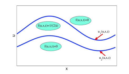
Figure 5: (color online) The water bag model. The electron distribution is confined between two limiting trajectories $u_{1,2}$.

3 The water bag model of driven-chirped plasma waves

The water bag model (Berk et al., 1970) assumes that the electron distribution function remains constant, $f(u,x,t)=1/(2\Delta)$, between two limiting trajectories $u_{1,2}(x,t)$ in phase space and vanishes outside these trajectories (see Fig. 5). Then the electron density is $n(x,t)=\int fdu=(u_{1}-u_{2})/(2\Delta)$ and our kinetic SPW problem is governed by the following set of the momentum and Poisson equations

$$u_{1t}+u_{1}u_{1x}=(\varphi+\varphi_{d})_{x},$$

$$u_{2t}+u_{2}u_{2x}=(\varphi+\varphi_{d})_{x},$$ (2)

$$\displaystyle\varphi_{xx}=\kappa^{2}\varphi+(u_{1}-u_{2})/(2\Delta)-1,$$

where we use the same normalization of $x,t,f,u_{1,2},\varphi,$ and $\varphi_{d}$ as in the previous section. We will be solving this system subject to $2\pi$ periodicity in $x$ for a trivial initial equilibrium $\varphi=0,$ $u_{1,2}=\pm\Delta$. Note that if one also defines $v(x,t)=(u_{1}+u_{2})/2$, Eqs. (3) yield

$$n_{t}+(vn)_{x}=0,$$

$$v_{t}+vv_{x}=(\varphi+\varphi_{d})_{x}-\Delta^{2}nn_{x},$$ (3)

$$\varphi_{xx}=\kappa^{2}\varphi+n-1.$$

Therefore, the water bag model is isomorphic to the usual warm fluid limit of the driven plasma waves with the adiabatic electron pressure scaling $p\sim n^{3}$ and $\Delta^{2}=3\sigma^{2}$. The results shown by the dotted red lines in Figs. 3 and 4 were obtained by solving Eqs. (3) numerically and show excellent agreement between the VP and water bag simulations until approaching the Landau resonance. These water bag simulations used a code similar to that for SIAWs (Friedland & Shagalov, 2017) and based on a standard spectral method (Canuto et al., 1988).

In analyzing the AR threshold in the problem, we use a Lagrangian approach. We introduce new potentials $\psi_{1,2}$ via $u_{1,2}=\pm\Delta+\partial_{x}\psi_{1,2}$ and rewrite Eqs. (3) as

$$\psi_{1tx}+\Delta\psi_{1xx}+\psi_{1x}\psi_{1xx}=(\varphi+\varphi_{d})_{x},$$

$$\psi_{2tx}-\Delta\psi_{2xx}+\psi_{2x}\psi_{2xx}=(\varphi+\varphi_{d})_{x},$$ (4)

$$\varphi_{xx}=\kappa^{2}\varphi+(\psi_{1x}-\psi_{2x})/2\Delta.$$

This system can be derived from the variation principle $\delta(\int Ldxdt)=0$, with the three-field Lagrangian density

$$L=\frac{1}{2}\varphi_{x}^{2}+\frac{\kappa^{2}\varphi^{2}}{2}-\frac{\psi_{1x}^{2}+\psi_{2x}^{2}}{4}-\frac{\psi_{1x}\psi_{1t}-\psi_{2x}\psi_{2t}}{4\Delta}$$

$$-\frac{\psi_{1x}^{3}-\psi_{2x}^{3}}{12\Delta}+\frac{(\psi_{1x}-\psi_{2x})(\varphi+\varphi_{d})}{2\Delta}.$$ (5)

Our next goal is to apply the Whitham’s averaged variational principle (Whitham, 1974) and derive weakly nonlinear slow evolution system describing driven-chirped SPWs governed by this Lagrangian. We proceed by discussing weakly nonlinear driven and phase-locked, but not chirped SPWs.

4 Weakly nonlinear SPWs

If one starts in the trivial equilibrium $\varphi=0,$ $n=1$, $v=0$ ($u_{1,2}=\pm\Delta$), Eqs. (3) after averaging over one spatial period, yield constant-in-time averaged density and fluid velocity $\left\langle n\right\rangle=1$, $\left\langle v\right\rangle=0$ ($\left\langle u_{1,2}\right\rangle=\pm\Delta$). We consider the linear stage of driven SPWs first, i.e., write $n=1+\delta n$ and linearize (3) to get

$$(\delta n)_{t}+v_{x}=0,$$

$$v_{t}=\varphi_{x}-\Delta^{2}\delta n_{x}-2\varepsilon\cos\theta_{d}\sin x,$$ (6)

$$\varphi_{xx}=\kappa^{2}\varphi+\delta n.$$

In the case of a constant driving frequency, this set yields phase-locked standing wave solutions of frequency $\omega=\omega_{d}$ for all dependent variables

$$\delta n=a\cos\theta\cos x,$$

$$v=b\sin\theta\sin x,$$ (7)

$$\varphi=c\cos\theta\cos x,$$

where $\theta=\theta_{d}=\omega t$,

$$a=-\frac{2\varepsilon}{\omega^{2}-\omega_{0}^{2}},$$

$$b=\omega a,$$ (8)

$$c=-\frac{a}{1+\kappa^{2}}.$$

and

$$\omega_{0}^{2}=\frac{1}{(1+\kappa^{2})}+\Delta^{2}.$$ (9)

Note that $\omega_{0}$ is the natural frequency of a linear SPW in the problem. Equations (7) yield the linear solutions

$$u_{1,2}=v\pm\Delta(1+\delta n)=\pm\Delta+b\sin\theta\sin x\pm\Delta a\cos\theta\cos x$$ (10)

and, thus,

$$\psi_{1,2}=-b\sin\theta\cos x\pm\Delta a\cos\theta\sin x.$$ (11)

Interestingly, in contrast to $n,u$, and $\varphi$, the linear solutions for $u_{1,2}$ and $\psi_{1,2}$ are not standing waves.

Our next goal is to include a weak nonlinearity in the problem, but still for a constant driving frequency case. To this end, we use spatial periodicity and write truncated Fourier expansions

$$\psi_{1,2}=b_{1,2}\cos x+a_{1,2}\sin x+d_{1,2}\cos(2x)+e_{1,2}\sin(2x),$$ (12)

$$\varphi=c_{1}\cos x+c_{2}\cos(2x),$$ (13)

where $a_{1,2}$, $b_{1,2}$, and $c_{1}$ are time dependent amplitudes viewed as small first order objects, while $d_{1,2}$, $e_{1,2}$, and $c_{2}$ are due to the nonlinearity and, thus, are of second order. The time dependence of the first order amplitudes is assumed to be that of the linear solutions (11) and (7), i.e. $a_{1,2}=A_{1,2}\cos\theta$, $b_{1,2}=B_{1,2}\sin\theta$, and $c_{1}=C_{1}\cos\theta$. But what is the time dependence of the second order amplitudes? Instead of working with the original system (3) for answering this question, we use a simpler Lagrangian approach in Appendix A. The final result is [see Eqs. (40)]

$$d_{1,2}=D_{1,2}\sin(2\theta)$$

$$e_{1,2}=F_{1,2}+E_{1,2}\cos(2\theta)$$ (14)

$$c_{2}=B+C\cos(2\theta)$$

where $D_{1,2}$, $F_{1,2}$, $E_{1,2}$, $B$, and $C$ are constants. Thus, the potentials characterizing a weakly nonlinear SPW phase-locked to the drive are:

$$\psi_{i}=B_{i}\sin\theta\cos x+A_{i}\cos\theta\sin x+D_{i}\sin(2\theta)\cos(2x)+[F_{i}+E_{i}\cos(2\theta)]\sin(2x),$$ (15)

$$\varphi=C_{1}\cos\theta\cos x+[B+C\cos(2\theta)]\cos(2x).$$ (16)

Here $i=1,2$, all the coefficients (amplitudes) are constant and could be related to the driving amplitude $\varepsilon$ by using the approach of Appendix A. Nevertheless, we will not follow this route because, knowing the form of Eqs. (15) and (16) is sufficient for addressing our original driven-chirped problem via the Whitham’s averaged variational principle (Whitham, 1974), as described next.

5 Whitham’s averaged variational principle for driven SPWs

As in the case of the standing IAWs (Friedland et al., 2019), the Whitham’s approach uses the ansatz of form (15) and (16) for the solution of our driven-chirped problem, but now all the amplitudes are viewed as slow functions of time and $\theta$ is the fast wave phase having a slowly varying frequency $\omega(t)=d\theta/dt$ generally different from the frequency $\omega_{d}(t)$ of the chirped driving wave. This ansatz is then substituted into the Lagrangian density (5), where the driver is written as $\varphi_{d}=2\varepsilon\cos(\theta+\Phi)\sin x$ and the phase mismatch $\Phi(t)=\theta_{d}-\theta$ is viewed as a slow function of time. Then, all the slow variables are frozen in time and the Lagrangian density is averaged over $2\pi$ in both $x$ and $\theta$ (fast scales). This results in a new averaged Lagrangian density $\Lambda$, which depends on slow objects only [i.e., $A_{1,2}$, $B_{1,2}$, $C_{1}$ (first order amplitudes), $D_{1,2}$, $E_{1,2}$, $F_{1,2}$, $B$, $C$ (second order amplitudes), the wave frequency $\omega$, and the phase mismatch $\Phi$]. To fourth order in amplitudes we obtain [via Mathematica (Wolfram Research Inc., 2017)] $\Lambda=\Lambda_{2}+\Lambda_{4}+\Lambda_{d}$, where

$$\Lambda_{2}=2C_{1}^{2}(1+\kappa^{2})-A_{1}^{2}-A_{2}^{2}-B_{1}^{2}-B_{2}^{2}$$

$$-\frac{2}{\Delta}[\omega(A_{1}B_{1}-A_{2}B_{2})-C_{1}(A_{1}-A_{2})],$$ (17)

$$\Lambda_{4}=-4(2F_{1}^{2}+2F_{2}^{2}+D_{1}^{2}+D_{2}^{2}+E_{1}^{2}+E_{2}^{2})$$

$$+2(4+\kappa^{2})(2B^{2}+C^{2})-\frac{4}{\Delta}[2\omega(D_{1}E_{1}-D_{2}E_{2})$$

$$+2B(F_{1}-F_{2})+C(E_{1}-E_{2})]-\frac{1}{\Delta}[A_{1}B_{1}D_{1}-A_{2}B_{2}D_{2}]$$

$$+\frac{1}{2\Delta}[B_{1}^{2}(2F_{1}-E_{1})-A_{1}^{2}(2F_{1}+E_{1})-B_{2}^{2}(2F_{2}-E_{2})+A_{2}^{2}(2F_{2}+E_{2})],$$ (18)

$$\Lambda_{d}=\frac{4\varepsilon}{\Delta}(A_{1}-A_{2})\cos\Phi.$$ (19)

Note that $\Lambda$ has an algebraic form with the wave phase $\theta$ entering via $\Phi=$ $\theta_{d}-\theta$ and $\omega(t)=d\theta/dt$. Therefore, the variations with respect to all amplitudes yield a set of eight algebraic equations

$$\frac{\partial\Lambda}{\partial Z_{i}}=0,i=1,..,8,$$ (20)

where $Z_{i}$ represent each of the $8$ slow amplitudes in the problem. In addition, the variation with respect to $\theta$ yields an ordinary differential equation (ODE)

$$\frac{d}{dt}\left(\frac{\partial\Lambda}{\partial\omega}\right)=-\frac{\partial\Lambda}{\partial\Phi}.$$ (21)

To lowest order, the last equation becomes

$$\frac{d}{dt}(A_{1}B_{1}-A_{2}B_{2})=-2\varepsilon(A_{1}-A_{2})\sin\Phi.$$ (22)

and, as expected, describes the slow evolution, provided $\varepsilon$ is sufficiently small.

The plan for analyzing our slow driven system is as follows. First, we will use the algebraic equations (20) for expressing seven of the eight amplitudes and $\omega$ in terms of $\Phi$ and the eighth amplitude (chosen to be $C_{1}$), i.e. obtain relations $Z_{i}=Z_{i}(C_{1},\Phi)$ and $\omega=\omega(C_{1},\Phi)$. Then

$$\frac{d\Phi}{dt}=\omega_{d}(t)-\omega(C_{1},\Phi),$$ (23)

which in combination with Eq. (22) comprise a closed set of two ODEs describing the slow evolution in our driven system. This plan is algebraically complex, but can be performed using Mathematica (Wolfram Research Inc., 2017). We describe the intermediate steps of this calculation in Appendix B and here present the final results. To lowest significant order, the amplitudes in Eq. (22) are as in the linear problem [see Eqs. (42), (43)]

$$A_{1}=-A_{2}\approx-\frac{C_{1}\Delta}{\omega_{0}^{2}-\Delta^{2}}=-C_{1}\Delta(1+\kappa^{2}),$$ (24)

$$B_{1}=B_{2}\approx\frac{C_{1}\omega_{0}}{\omega_{0}^{2}-\Delta^{2}}=C_{1}\omega_{0}(1+\kappa^{2}),$$ (25)

while [see Eqs. (49) and (50) in Appendix B]

$$\omega^{2}(C_{1},\Phi)\approx\omega_{0}^{2}+NC_{1}^{2}+\frac{2\varepsilon\cos\Phi}{(1+\kappa^{2})C_{1}},$$ (26)

where

$$N=\frac{9\kappa^{2}(3+\kappa^{2})+R}{96[1+(4+\kappa^{2})\Delta^{2}]},$$ (27)

and $R=(1+\kappa^{2})\Delta^{2}[3(60+56\kappa^{2}+11\kappa^{4})+20(1+\kappa^{2})(4+\kappa^{2})(5+2\kappa^{2})\Delta^{2}+16(1+\kappa^{2})^{2}(4+\kappa^{2})^{2}\Delta^{4}]$.

6 Dynamics and control of chirped-driven SPWs

At this stage, we discuss the slow evolution in our driven-chirped SPWs system. Upon substitution of Eqs. (24) and (25) into Eq. (22), we obtain

$$\frac{dC_{1}}{dt}=-\frac{\varepsilon}{\omega_{0}(1+\kappa^{2})}\sin\Phi.$$ (28)

Next, for a small frequency deviation in the vicinity of the linear resonance, $\omega=\omega_{0}+\delta\omega$, Eq. (26) yields

$$\delta\omega\approx\frac{N}{2\omega_{0}}C_{1}^{2}+\frac{\varepsilon\cos\Phi}{\omega_{0}(1+\kappa^{2})C_{1}},$$ (29)

where the two terms on the right represent the wave frequency shifts due to the nonlinearity and interaction, respectively. Then, from Eq. (23) and using the driving frequency $\omega_{d}=\omega_{0}+\alpha t$, we obtain

$$\frac{d\Phi}{dt}=\alpha t-\frac{N}{2\omega_{0}}C_{1}^{2}-\frac{\varepsilon\cos\Phi}{\omega_{0}(1+\kappa^{2})C_{1}}.$$ (30)

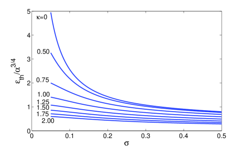
Figure 6: (color online) The rescaled threshold driving amplitude $\varepsilon_{th}/\alpha^{3/4}$ versus $\sigma=k\lambda_{D}$ for different values of the screening parameter $\kappa$

Equations (28) and (30) comprise a complete set of amplitude-phase mismatch ODEs describing the passage through the linear resonance in our problem. These equations involve several parameters, but the number of parameters can be reduced to just one by rescaling the problem. Indeed, if we use the slow time $\tau=\alpha^{1/2}t$ and define new amplitude $Q$ via $Q^{2}=\frac{N}{2\omega_{0}\alpha^{1/2}}C_{1}^{2}$, our system reduces to

$$\frac{dQ}{d\tau}=-\mu\sin\Phi,$$ (31)

$$\frac{d\Phi}{d\tau}=\tau-Q^{2}-\frac{\mu\cos\Phi}{Q}.$$ (32)

where

$$\mu=\frac{\varepsilon N^{1.2}}{\sqrt{2}\alpha^{3/4}\omega_{0}^{3/2}(1+\kappa^{2})}.$$ (33)

Note that, if one defines a complex variable $\Psi=Qe^{i\Phi}$, our system is further reduced to a single complex ODE

$$i\Psi_{\tau}+(\tau-|\Psi|^{2})\Psi=\mu$$ (34)

characteristic to AR problems in many different physical systems and studied in numerous application (Friedland, 2009). For example, if initially $\Psi=0$ and one starts at sufficiently large negative $\tau$ (i.e. far from the linear resonance), this equation predicts transition to AR at large positive $\tau$ if $\mu$ is above the threshold $\mu_{th}\approx 0.41$, or returning to our original parameters,

$$\varepsilon>\varepsilon_{th}=0.58\frac{\alpha^{3/4}\omega_{0}^{3/2}(1+\kappa^{2})}{N^{1.2}}.$$ (35)

The threshold (35) assumes its simplest form when either $\Delta$ or $\kappa$ vanish. Indeed, in the cold plasma case, $\Delta=0$ and

$$N=\frac{3\kappa^{2}(3+\kappa^{2})}{32}.$$ (36)

Therefore, for small $\kappa$, $\varepsilon_{th}$ scales as $\varepsilon_{th}\sim\alpha^{3/4}/\kappa$ and one needs a non-vanishing screening factor $\kappa$ to get a sufficiently small $\varepsilon_{th}$ for the AR excitation. In the case of $\kappa=0$ and $\Delta\ll 1$,

$$N\approx\frac{15\Delta^{2}}{8},$$ (37)

so $\varepsilon_{th}$ scales as $\varepsilon_{th}\sim\alpha^{3/4}/\Delta$ (recall that $\Delta=3^{1/2}k\lambda_{D}$ and measures the electron thermal spread in the problem). We illustrate these results in Fig. 6 showing $\varepsilon_{th}/\alpha^{3/4}$ vs $\sigma$ (this is $k\lambda_{D}$ in dimensional notations) for several values of $\kappa$.

Figure 7: (color online) The control of the autoresonant SPW by tapering the driving frequency. Panel (a): The envelope of the maxima of the electron fluid velocity $v$ versus slow time $\tau=\alpha^{1/2}t$. The dashed line represents the phase velocity $\omega_{d}/k$ of the driving wave and the dotted red line represents the envelope of the maxima of the upper limiting velocity of the water bag model. Panel (b) shows the frequencies of the driving (red line) and driven (blue line) waves. The waves are frequency locked starting $\tau\approx-3$.

Finally, we address the possibility of autoresonant control of large amplitude SPWs. This control uses a one-to-one correspondence between the amplitude and frequency of nonlinear waves. Since in autoresonance the driven wave frequency is locked to the driving frequency, the wave amplitude can be controlled by simply varying the driving frequency. For example, we have seen previously (see Fig. 3), that a continuous linear time variation of the driving frequency leads to the excited wave approaching the wave breaking limit. But what if one wants to avoid this limit and excite a wave having some given target amplitude? This goal can be achieved by tailoring the time variation of the driving frequency appropriately. We illustrate such control in Fig. 7 showing the results of the simulations using the water bag model for the case of $\sigma=0.05$, $\kappa=0.75$, $\varepsilon=0.0011$ ($\varepsilon_{th}=0.00084$ in this case) and the driving frequency $\omega_{d}=\omega_{0}+\alpha t$ for $t<0$, but $\omega_{d}=\omega_{0}+\frac{2d}{\pi}arctg(t/T)$ for $t>0$, where $T=$ $\frac{2d}{\pi\alpha}$. This driving frequency approaches a fixed value of $\omega_{0}+d$ at large times (we used $d=0.033$ in the simulations). Fig. 7a shows the envelopes of the maxima of the electron fluid velocity $v$ (solid line) and of the upper limiting velocity $u_{1}$ of the water bag model (dotted line). In the same figure, we also show the driving wave phase velocity (dashed line). Separate simulations show that if the driving frequency in this example is chirped linearly in time, the upper limiting velocity of the water bag approaches the Landau resonance ($u_{1}\approx\omega_{d}/k$) at $\tau=6$, where wave breaking is expected. In contrast, for the saturated driving frequency case shown in Fig. 7, the excited fluid velocity also saturates at larger times and performs slow oscillations around some fixed value. The frequency of these oscillations scales as $\varepsilon^{1/2}$ (Friedland, 2009) and their presence illustrates stability of the AR evolution. The velocity $u_{1}$ also saturates and, thus, the kinetic wave breaking is avoided. This saturation is caused by the autoresonant frequency locking in the system as illustrated in Fig. 7b, showing the evolution of the frequencies of the driven and driving waves.

7 Conclusions

We have studied excitation and control of large amplitude SPWs by a chirped frequency driving wave. The process involved passage through the linear resonance in the problem and transition to autoresonant stage of excitation, where the driven SPW self-adjusts its amplitude to stay in a continuous resonance with the drive. The method allowed reaching extreme regimes, where the electron density developed a sharply peaked spatial profile with the maximum electron density exceeding the initial plasma density significantly (see Fig. 1). These results were illustrated in both Vlasov-Poisson and water bag simulations. The simpler water bag model [Eqs. (3)] was used for developing the adiabatic theory using the Whitham’s averaged variational principle for studying the weakly nonlinear stage of formation of autoresonant SPWs. In this regime, the problem was reduced to the standard set of coupled amplitude-phase mismatch equations (31) and (32) characteristic to many other autoresonantly driven problems. The reduction also allowed finding the threshold driving amplitude [see Eq. (35)] for the transition to autoresonance. By slowly decreasing the chirp rate of the driving frequency and reaching some fixed frequency level, one could arrive at a given target amplitude of the autoresonant SPW and avoid the kinetic wave breaking (see Fig. 7).

The self-consistent inclusion of the variation of the driving amplitude and of 3D effects in the process of autoresonant excitation of SPWs seem to be an important goals for future research. The form of the autoresonant SPW suggests that it comprises a two-phase solution, with each phase locked to one of the traveling waves comprising the drive. A better understanding of such waveforms, analyzing other autoresonant multi-phase plasma waves, and studying details of the kinetic wave breaking process in application to autoresonant SPWs also comprise interesting goals for the future.

Appendix A Second order amplitudes

For calculating the second order amplitudes, we substitute Eqs. (12) and (13) into the Lagrangian (5), write the result to second nonlinear order in amplitudes and average over one spatial period. This spatially averaged Lagrangian governs the time dependence of all the amplitudes. Its variations with respect to the second order amplitudes yield a system of ODEs for these amplitudes versus time. Algebraically, this reduction is a tedious process done here using Mathematica (Wolfram Research Inc., 2017). The resulting set of equations is

$$(e_{1,2})_{t}=\frac{1}{2}(a_{1,2}b_{1,2}\pm 4\Delta d_{1,2}),$$

$$(d_{1,2})_{t}=\frac{1}{4}(4c_{2}-a_{1,2}^{2}+b_{1,2}^{2}\mp 8\Delta e_{1,2}),$$ (38)

$$c_{2}=\frac{e_{2}-e_{1}}{\Delta(4+\kappa^{2})},$$

or after substituting the first order dependencies $a_{1,2}\sim\cos\theta$, $b_{1,2}\sim\sin\theta$, and $c_{1}\sim\cos\theta$

$$(e_{1,2})_{t}=p_{1,2}\sin(2\theta)\pm 2\Delta d_{1,2},$$

$$(d_{1,2})_{t}=q_{1,2}+r_{1,2}\cos(2\theta)+c_{2}\mp 2\Delta e_{1,2},$$ (39)

$$c_{2}=\frac{e_{2}-e_{1}}{\Delta(4+\kappa^{2})},$$

where $p_{1,2}$, $q_{1,2}$, $r_{1,2}$ are constants. These equations have the following time periodic solutions

$$d_{1,2}=D_{1,2}\sin(2\theta),$$

$$e_{1,2}=F_{1,2}+E_{1,2}\cos(2\theta),$$ (40)

$$c_{2}=B+C\cos(2\theta).$$

where $D_{1,2}$, $F_{1,2}$, $E_{1,2}$, $B$, and $C$ are constants.

Appendix B The reduction of the variational system

All algebraic manipulations in this Appendix use Mathematica (Wolfram Research Inc., 2017). We employ the averaged Lagrangian $\Lambda$ [see Eqs. (17)-(19)] and proceed from the variations with respect to the first order amplitudes $A_{1,2}$, $B_{1,2}$, $C_{1}$:

$$-2C_{1}+2A_{1}F_{1}+B_{1}D_{1}+A_{1}E_{1}+2B_{1}\omega+2A_{1}\Delta=4\varepsilon\cos\Phi,$$

$$-2C_{1}+2A_{2}F_{2}+B_{2}D_{2}+A_{2}E_{2}+2B_{2}\omega-2A_{2}\Delta=4\varepsilon\cos\Phi,$$

$$2F_{1}B_{1}-A_{1}(D_{1}+2\omega)-B_{1}(E_{1}+2\Delta)=0,$$ (41)

$$-2F_{2}B_{2}+A_{2}(D_{2}+2\omega)+B_{2}(E_{2}-2\Delta)=0,$$

$$A_{1}-A_{2}+2C_{1}(1+\kappa^{2})\Delta=0.$$

The first four equations in this set yield the linear approximation in terms of $C_{1}$

$$A_{1}^{\prime}=-A_{2}^{\prime}=-\frac{C_{1}\Delta}{\omega^{2}-\Delta^{2}},$$ (42)

$$B_{1}^{\prime}=B_{2}^{\prime}=\frac{C_{1}\omega}{\omega^{2}-\Delta^{2}}.$$ (43)

Then the fifth equation in Eq. (41) gives the linear dispersion relation

$$\omega_{0}^{2}=\frac{1}{1+\kappa^{2}}+\Delta^{2}.$$ (44)

Next, we take variations with respect to the second order amplitudes $D_{1,2}$, $E_{1,2}$, $F_{1,2}$, $B$, $C$ (to lowest significant order using the linear result for the first order amplitudes and $\omega$) to get

$$A_{1}^{\prime}B_{1}^{\prime}+8E_{1}\omega_{0}+8D_{1}\Delta=0,$$

$$A_{2}^{\prime}B_{2}^{\prime}+8E_{2}\omega_{0}-8D_{2}\Delta=0,$$

$$-8C0+A_{1}^{\prime 2}+B_{1}^{\prime 2}+16D_{1}\omega_{0}+16E_{1}\Delta=0,$$

$$-8C0+A_{2}^{\prime 2}+B_{2}^{\prime 2}+16D_{2}\omega_{0}-16E_{2}\Delta=0,$$ (45)

$$8B-A_{1}^{\prime 2}+B_{1}^{\prime}-16F_{1}\Delta=0,$$

$$8B-A_{2}^{\prime 2}+B_{2}^{\prime 2}+16F_{2}\Delta=0,$$

$$F_{1}-F_{2}+B(4+\kappa^{2})\Delta=0,$$

$$E_{1}-E_{2}+C(4+\kappa^{2})\Delta=0,$$

This system is now solved for the second order amplitudes via $C_{1}^{2}$:

$$D_{1}=\frac{C_{1}^{2}\omega_{0}[2+\omega_{0}^{2}(4+\kappa^{2})+3\Delta^{2}(4+\kappa^{2})]}{16(\omega_{0}^{2}-\Delta^{2})^{2}[1-\omega_{0}^{2}(4+\kappa^{2})+\Delta^{2}(4+\kappa^{2})]},$$

$$E_{1}=-\frac{C_{1}^{2}\Delta[3\omega_{0}^{2}(4+\kappa^{2})+\Delta^{2}(4+\kappa^{2})]}{16(\omega_{0}^{2}-\Delta^{2})^{2}[1-\omega_{0}^{2}(4+\kappa^{2})+\Delta^{2}(4+\kappa^{2})]},$$

$$F_{1}=\frac{C_{1}^{2}(4+\kappa^{2})\Delta}{16(\omega_{0}^{2}-\Delta^{2})[1+\Delta^{2}(4+\kappa^{2})]},$$ (46)

$$D_{2}=D_{1},E_{2}=-E_{1},F_{2}=-F_{1},$$

$$B=-\frac{C_{1}^{2}}{8(\omega_{0}^{2}-\Delta^{2})[1+\Delta^{2}(4+\kappa^{2})]},$$

$$C=\frac{C_{1}^{2}(3\omega_{0}^{2}+\Delta^{2})}{8(\omega_{0}^{2}-\Delta^{2})^{2}[1-\omega_{0}^{2}(4+\kappa^{2})+-\Delta^{2}(4+\kappa^{2})]}.$$

Finally, we return to the first two equations in (41) and solve these equations for $A_{1,2}$ to higher (third) order in $C_{1}$

$$A_{1}^{\prime\prime}=-\frac{C_{1}\Delta}{\omega^{2}-\Delta^{2}}+\frac{C_{1}G_{1}-4\varepsilon\Delta(\omega_{0}^{2}-\Delta^{2})\cos\Phi}{2(\omega_{0}^{2}-\Delta^{2})^{2}},$$ (47)

$$A_{2}^{\prime\prime}=\frac{C_{1}\Delta}{\omega^{2}-\Delta^{2}}+\frac{C_{1}G_{2}+4\varepsilon\Delta(\omega_{0}^{2}-\Delta^{2})\cos\Phi}{2(\omega_{0}^{2}-\Delta^{2})^{2}},$$ (48)

where $G_{1}=\omega_{0}^{2}(2F_{1}-E_{1})+2D_{1}\omega_{0}\Delta-\Delta^{2}(2F_{1}+E_{1})$ and $G_{2}=\omega_{0}^{2}(2F_{2}-E_{2})-2D_{2}\omega_{0}\Delta-\Delta^{2}(2F_{2}+E_{2})$. Finally, we use Eqs. (46) in Eqs. (47) and (48) and substitute the resulting $A_{1,2}^{\prime\prime}$ into the last equation in (41). This yields a higher order approximation for the frequency $\omega$ of the wave:

$$\omega^{2}=\omega_{0}^{2}+NC_{1}^{2}+\frac{2\varepsilon\cos\Phi}{(1+\kappa^{2})C_{1}},$$ (49)

where

$$N=\frac{9\kappa^{2}(3+\kappa^{2})+R}{96[1+(4+\kappa^{2})\Delta^{2}]},$$ (50)

and $R=(1+\kappa^{2})\Delta^{2}[3(60+56\kappa^{2}+11\kappa^{4})+20(1+\kappa^{2})(4+\kappa^{2})(5+2\kappa^{2})\Delta^{2}+16(1+\kappa^{2})^{2}(4+\kappa^{2})^{2}\Delta^{4}]$.

References

- Berk et al. (1970) Berk, H., Nielsen, C. & Roberts, K. 1970 Phase space hydrodynamics of equivalent nonlinear systems: experimental and computational observations. Phys. Fluids 13, 980–995.
- Canuto et al. (1988) Canuto, C., Hussaini, M., Quarteroni, A. & Zang, T. 1988 Spectral Methods in Fluid Dynamics. Springer-Verlag.
- Dubin & Ashourvan (2015) Dubin, D. & Ashourvan, A. 2015 Trivelpiece-gould waves: frequency, functional form, and stability. Phys. Plasmas 22, 102102.
- Fajans & Friedland (2001) Fajans, J. & Friedland, L. 2001 Autoresonant (nonstationary) excitation of pendulums, plutinos, plasmas, and other nonlinear oscillators. Am. J. Phys. 69, 1096–1102.
- Friedland (2009) Friedland, L. 2009 Autoresonance in nonlinear systems. Scholarpedia 4, 5473.
- Friedland et al. (2006) Friedland, L., Khain, P. & Shagalov, A. 2006 Autoresonant phase-space holes in plasmas. Phys. Rev. Lett. 96, 225001.
- Friedland et al. (2019) Friedland, L., Marcus, G., Wurtele, J. & Michel, P. 2019 Excitation and control of large amplitude standing ion acoustic waves. Phys. Plasmas 26, 092109.
- Friedland & Shagalov (2014) Friedland, L. & Shagalov, A. 2014 Excitation and control of chirped nonlinear ion-acoustic waves. Phys. Rev. E 97, 063201.
- Friedland & Shagalov (2017) Friedland, L. & Shagalov, A. 2017 Extreme driven ion acoustic wavess. Phys. Plasmas 24, 082106.
- Lehmann & Spatachek (2016) Lehmann, G. & Spatachek, K. 2016 Transient plasma photonic crystals for high-power lasers. Phys. Rev. Lett. 116, 225002.
- Lehmann & Spatschek (2018) Lehmann, G. & Spatschek, K. 2018 Hamiltonian stochastic processes induced by succesive wave-particle interactions in stimulated raman scattering. Phys. Rev. E 79, 046404.
- Malkin et al. (1999) Malkin, V., Shvets, G. & Fisch, N. 1999 Fast compression of laser beams to highly overcritical power. Phys. Rev. Lett. 82, 4448–4451.
- Michel et al. (2014) Michel, P., Divol, L., Turnbull, D. & Moody, J. 2014 Dynamic control of the polarization of intense laser beams via optical wave mixing in plasmas. Phys. Rev. Lett. 113, 205001.
- Michel et al. (2009) Michel, P., Divol, L., Williams, E., Weber, S., Thomas, C., Callahan, D., Haan, S., Salmonson, J., Dixit, S., Hinkel, D., Edwards, M., Macgowan, B., Lindl, J., Glenzer, S. & Suter, L. 2009 Tuning the implosion symmetry of icf targets via controlled crossed-beam energy transfer. Phys. Rev. Lett. 102, 025004.
- Novikov et al. (1984) Novikov, S., Manakov, S., Pitaevskii, L. & Zakharov, V. 1984 Theory of solitons. Plenum Publishing.
- Turnbull et al. (2017) Turnbull, D., Goyon, C., Kemp, G., Pollock, B., Mariscal, D., Divol, L., Ross, J., Patankar, S., Moody, J. & Michel, P. 2017 Refractive index seen by a probe beam interacting with a laser-plasma system. Phys. Rev. Lett. 118, 015001.
- Turnbull et al. (2016) Turnbull, D., Michel, P., Chapman, T., Tubman, E., Pollock, B., Chen, C., Goyon, C., Ross, J., Divol, L., Woolsey, N. & Moody, J. 2016 High power dynamic polarization control using plasma photonics. Phys. Rev. Lett. 116, 205001.
- Whitham (1974) Whitham, G. 1974 Linear and Nonlinear Waves. John Wiley & Sons.
- Wolfram Research Inc. (2017) Wolfram Research Inc. 2017 Mathematica. Version 11.1 .