NWPU-Crowd: A Large-Scale Benchmark for Crowd Counting and Localization

Abstract

In the last decade, crowd counting and localization attract much attention of researchers due to its wide-spread applications, including crowd monitoring, public safety, space design, etc. Many Convolutional Neural Networks (CNN) are designed for tackling this task. However, currently released datasets are so small-scale that they can not meet the needs of the supervised CNN-based algorithms. To remedy this problem, we construct a large-scale congested crowd counting and localization dataset, NWPU-Crowd, consisting of $5,109$ images, in a total of $2,133,375$ annotated heads with points and boxes. Compared with other real-world datasets, it contains various illumination scenes and has the largest density range ($0\!\sim\!20,033$). Besides, a benchmark website is developed for impartially evaluating the different methods, which allows researchers to submit the results of the test set. Based on the proposed dataset, we further describe the data characteristics, evaluate the performance of some mainstream state-of-the-art (SOTA) methods, and analyze the new problems that arise on the new data. What’s more, the benchmark is deployed at https://www.crowdbenchmark.com/, and the dataset/code/models/results are available at https://gjy3035.github.io/NWPU-Crowd-Sample-Code/.

1 Introduction

Crowd analysis is an essential task in the field of video surveillance. Accurate analysis for crowd motion, human behavior, population density is crucial to public safety, urban space design, etc. Crowd counting and localization are fundamental tasks in the field of crowd analysis, which serve high-level tasks, such as crowd flow estimation [1] and pedestrian tracking [2]. Due to the importance of crowd counting, many researchers [3, 4, 5] pay attention to it and achieve quite a few significant improvements in this field. Especially, benefiting from the development of deep learning in computer vision, the counting performance on the datasets [6, 7, 8, 9] is continuously refreshed by Convolutional Neural Networks (CNN)-based methods [10, 11, 12].

The CNN-based methods need to learn discriminate features from a multitude of labeled data, so a large-scale dataset can effectively promote the development of visual technologies. It is verified in many existing tasks, such as object detection [13] and semantic segmentation [14]. However, the currently released crowd counting datasets are so small-scale that most deep-learning-based methods are prone to overfit the data. According to the statistics, UCF-QNRF [9] is the largest released congested crowd counting dataset. Still, it contains only $1,535$ samples, in a total of $1.25$ million annotated instances, which is still unable to meet the needs of current deep learning methods. Moreover, some works [9, 15] focus on the crowd localization task that produces point-wise predictions for each instance. However, the traditional datasets do not contain box-level labels, which makes it hard to evaluate the localization performance using a uniform metric. Furthermore, there is not an impartial evaluation benchmark, which potentially restricts further development of crowd counting. By the way, some methods may use mistaken labels to evaluate models, which is also not accurate. Reviewing some benchmarks in other fields, CityScapes [16] and Microsoft COCO [13], they allow the researchers to submit their results of the test set and impartially evaluate them, which facilitates the study of methodology. Thus, an equitable evaluation platform is important for the community.

Considering the problems mentioned above, in this paper, we construct a large-scale crowd counting and localization dataset, named as NWPU-Crowd, and develop a benchmark website to boost the community of crowd analysis. Compared with the existing congested datasets, the proposed NWPU-Crowd has the following main advantages: 1) This is the largest crowd counting and localization dataset, consisting of $5,109$ images and containing $2,133,375$ annotated instances; 2) It introduces some negative samples like high-density crowd images to assess the robustness of models; 3) In NWPU-Crowd, the number of annotated objects range, $0\sim 20,033$. More concrete features are described in Section 3.3. Table I illustrates the detailed statistics of ten mainstream real-world datasets and the proposed NWPU-Crowd.

TABLE I: Statistics of the ten mainstream crowd counting datasets and NWPU-Crowd.

Dataset	Number	Avg. Resolution	Count Statistics				Extreme	Unseen	Category-wise	Box-level
	of Images	($H\times W$)	Total	Min	Ave	Max	Congestion	Test Labels	Evaluation	Label
UCSD [6]	2,000	$158\times 238$	49,885	11	25	46	✗	✗	✗	✗
Mall [17]	2,000	$480\times 640$	62,325	13	31	53	✗	✗	✗	✗
WorldExpo’10 [8]	3,980	$576\times 720$	199,923	1	50	253	✗	✗	✔	✗
ShanghaiTech Part B [7]	716	$768\times 1024$	88,488	9	123	578	✗	✗	✗	✗
Crowd_Surv [18]	13,945	$840\times 1342$	386,513	2	35	1,420	✗	✗	✗	✗
UCF_CC_50 [19]	50	$2101\times 2888$	63,974	94	1,279	4,543	✔	✗	✗	✗
ShanghaiTech Part A [7]	482	$589\times 868$	241,677	33	501	3,139	✔	✗	✗	✗
UCF-QNRF [9]	1,535	$2013\times 2902$	1,251,642	49	815	12,865	✔	✗	✗	✗
GCC (synthetic) [20]	15,212	$1080\times 1920$	7,625,843	0	501	3,995	✔	✗	✔	✗
JHU-CROWD++ [21, 22]	4,372	$910\times 1430$	1,515,005	0	346	25,791	✔	✗	✔	✔
NWPU-Crowd	5,109	$\boldsymbol{2191\times 3209}$	2,133,375	0	418	20,033	✔	✔	✔	✔

Based on the proposed NWPU-Crowd, several experiments of some classical and state-of-the-art methods are conducted. After further analyzing their results, an interesting phenomenon on the proposed dataset is found: diverse data makes it difficult for counting networks to learn useful and distinguishable features, which does not appear or is ignored in the previous datasets. Specifically, 1) there are many error estimations on negative samples; 2) the data of different scene attributes (density level and luminance) have a significant influence on each other. Therefore, it is a research trend on how to alleviate the above two problems. What’s more, for localization task, we design a reasonable metric and provide some simple baseline models.

In summary, we believe that the proposed large-scale dataset will promote the application of crowd counting and localization in practice and attract more attention to tackling the aforementioned problems.

2 Related Works

The existing crowd counting datasets mainly contain two types: surveillance-scene datasets and general-scene datasets. The former commonly records crowd in particular scenarios, of which the data consistency is obvious. For the latter, the crowd samples are collected from the Internet. Thus, there are more perspective variations, occlusions, and extreme congestion in these datasets. Tabel I demonstrates a summary of the basic information of the mainstream crowd counting datasets, and in the following parts, their unique characters are briefly introduced.

2.1 Surveillance-scene Dataset

Surveillance view. Surveillance-view datasets aim to collect the crowd images in specific indoor scenes or small-area outdoor locations, such as marketplace, walking street, and station. The number of people usually ranges from 0 to 600. UCSD is a typical dataset for crowd analysis. It contains $2,000$ image sequences, which records a pedestrian walk-way at the University of California at San Diego (UCSD). Mall [17] is captured in a shopping mall with more perspective distortion. However, these two datasets contain only a single scene, lacking data diversity. Thus, Zhang et al. [8] build a multi-scene crowd counting dataset, WorldExpo’10, consisting of 108 surveillance cameras with different locations in Shanghai 2010 WorldExpo, e.g., entrance, ticket office. Considering the poor resolution of traditional surveillance cameras, Zhang et al. [7] construct a high-quality crowd dataset, ShanghaiTech Part B, containing $782$ images captured in some famous resorts of Shanghai, China. To remedy the occlusion problem in congested scenes, a multi-view dataset is designed by Zhang and Chan [23]. By equipping 5 cameras at different positions for a specific view, the data can be recorded synchronously. For getting rid of the manually labeling process, Wang et al. [20] construct a large-scale synthetic dataset (GCC). By simulating the perspective of a surveillance camera, they capture $400$ crowd scenes in a computer game (Grand Theft Auto V, GTA V), a total of $15,212$ images. The main advantage of GCC is that it can provide accurate labels (point and mask) and diverse environments. However, there are many domain shifts/gaps between synthetic and real data, limiting their practical values. Therefore, it is necessary to build a large-scale real-world dataset. Compared with GCC, the advantages of NWPU-Crowd are: more natural person models, crowd scenes and environment (weathers, light, etc.).

In addition to the aforementioned datasets, there are also other crowd counting datasets with their specific characteristics. SmartCity [24] focuses on some typical scenes, such as sidewalk and subway. ShanghaiTechRGBD [25] records the RGBD crowd images with a stereo camera for concentrating on pedestrian counts and localization. Fudan-ShanghaiTech [26] and Venice [27] capture the video sequences for temporal crowd counting.

Drone view. For some big scenes (such as stadium, plaza) or some large rally events (ceremony, hajj, etc.), the above traditional fixed surveillance camera is not suitable due to its small field of view. To tackle this problem, some other datasets are collected through the Drone or Unmanned Aerial Vehicle (UAV). Benefiting from their higher altitudes, more flexible view and free flight, more large scenes can be recorded compared with the traditional surveillance camera. There are two crowd counting datasets with the drone view, DLR-ACD Dataset [28] and DroneCrowd Dataset [29]. The former consists of 33 images with $226,291$ annotated persons, including some mass events: sports, concerts, trade fair, etc. The latter consists of $70$ crowd scenes , with a total of $33,600$ drone-view image sequences. Due to the Bird’s-Eye View (BEV), the whole body of pedestrians can not be seen except their heads, so the perspective change rarely appears in the above two datasets.

Figure 1: The display of the proposed NWPU-Crowd dataset. Column 1 shows some typical samples with normal lighting. The second and third column demonstrate the crowd scenes under the extreme brightness and low-luminance conditions, respectively. The last column illustrates the negative samples, including some scenes with densely arranged other objects.

2.2 General-scene Dataset

In addition to the above crowd images captured in specific scenes, there are also many general-scene crowd counting datasets, which are collected from the Internet. A remarkable aspect of general-scene is that the crowd density varies significantly, which ranges from $0$ to $20,000$. Besides, diversified scenarios, light and shadow conditions, and uneven crowd distribution in one single image are also distinctive attributes of these datasets.

The first general-scene dataset for crowd counting, UCF_CC_50 [19], is presented by Idrees et al. in 2013. It only contains $50$ images, which is so small to train a robust deep learning model. Consequently, a larger crowd counting dataset becomes more significant nowadays. Zhang et al. propose ShanghaiTech Part A [7], which is constructed of $482$ images crawled from the Internet. Although its average number of labeled heads in each image is smaller than UCV_CC_50, it contains more pictures and larger number of labeled head points. For further research on the extremely congested crowd counting, UCF-QNRF [9] is presented by Idrees et al. It is composed of $1,525$ images with more than $1,251,642$ label points. The average number of pedestrians per image is $815$, and the maximum number reaches $12,865$. Aiming at the small size of crowd images, Crowd Surveillance [18] build a large-scale dataset containing $13,945$ images, which provides regions of interest (ROI) for each image to keep out these blobs that are ambiguous for training or testing. In addition to the above datasets, Sindagi et al. introduce a new dataset for unconstrained crowd counting, JHU-CROWD, including $4,250$ samples. All images are annotated from the image and head level. For the former level, they label the scenario (mall, stadium, etc.) and weather conditions. For the head level, the annotation information includes not only head locations but also occlusion, size, and blur attributes.

3 NWPU-Crowd Dataset

This section describes the proposed NWPU-Crowd from four perspectives: data collection/specification, annotation tool, statistical analysis, data split and evaluation protocol.

3.1 Data Collection and Specification

Data Source. Our data are collected from self-shooting and the Internet. For the former, $\sim\!2,000$ images and $\sim\!200$ video sequences are captured in some populous Chinese cities, including Beijing, Shanghai, Chongqing, Xi’an, and Zhengzhou, containing some typical crowd scenes, such as resort, walking street, campus, mall, plaza, museum, station. However, extremely congested crowd scenes are not the norm in real life, which is hard to capture via self-shooting. Therefore, we also collect $\sim\!8,000$ samples from some image search engines (Google, Baidu, Bing, Sougou, etc.) via the typical query keywords related to the crowd. Table II lists the primary data source websites and the corresponding keywords. The third row in the table records some Chinese websites and keywords. Finally, by the above two methods, $10,257$ raw images are obtained.

TABLE II: The query keywords on some typical search engines.

Data Source	Keywords
	Crowd	Negative Sample
google, baidu, bing, pxhere, pixabay…	crowd, congestion, hundreds/thousands of people, speech, conference, ceremony, stadium, gathering, parade, demonstration, protest, carnival, beer festival, hajj, NBA, WorldCup, NFL, EPL, Super Bowl, etc.	dense, migration, fish school, empty scenes, flowers, etc.
baidu, weibo, sogou, so, wallhere…	人群，拥挤，春运，军训，典礼，祭祀，庙会， 游客，万人，千人，大赛，运动会，候车厅， 音乐会/节，见面会，人从众，黄金周，招聘会， 万人空巷，人山人海，摩肩接踵，水泄不通……	礼堂，动物迁徙， 花海，动漫人物， 餐厅，空无一人， 密集排列……

Data Deduplication and Cleaning. We employ four individuals to download data from the Internet on non-overlapping websites. Even so, there are still some images that contain the same content. Besides, some congested datasets (UCF_CC_50, Shanghai Tech Part A, and UCF-QNRF), are also crawled from the Internet, e.g., Flickr, Google, etc. For avoiding the problem of data duplication, we perform an effective strategy to measure the similarity between two images, which is inspired by Perceptual Loss [30]. Specifically, for each image, the layer-wise VGG-16 [31] features (from conv1 to conv5_3 layer) are extracted. Given two resized samples $i_{x}$ and $i_{y}$ with the resolution of $224\times 224$, the similarity is defined as follows:

$$\scriptsize\begin{array}[]{l}\begin{aligned} D\left({{i_{x}},{i_{y}}}\right)=\sum\limits_{j\in L}{\frac{1}{{{C_{j}}{H_{j}}{W_{j}}}}}\left\|{{\psi_{j}}({i_{x}})-{\psi_{j}}({i_{y}})}\right\|_{2}^{2},\end{aligned}\end{array}$$ (1)

where $L$ is the set of the last activation layer in five groups of VGG-16 network, namely $L=\left\{{{\psi_{j}}|j=1,2,...,5}\right\}=\left\{{relu1\_2,relu2\_2,relu3\_3,relu4\_3,relu5\_3}\right\}$. ${\psi_{j}}({i_{x}})$ and ${\psi_{j}}({i_{y}})$ denote layer ${\psi_{j}}$’s outputs (feature maps) for sample $i_{x}$ and $i_{y}$, respectively. ${C_{j}}$, ${H_{j}}$ and ${W_{j}}$ are the size of ${\psi_{j}}({i_{x}})$ at three axes: channel, height and width. If $D\left({{i_{x}},{i_{y}}}\right)<5$, these two samples are considered to have similar contents. As a result, one of the two is removed from the dataset.

Then remove excess similar images by computing the distance of the feature between any two samples. Furthermore, some blurred images that are difficult to recognize the head location are also removed. Consequently, we obtain $5,109$ valid images.

3.2 Data Annotation

Annotation tools: For conveniently annotating head points in the crowd images, an online efficient annotation tool is developed based on HTML5 + Javascript + Python. This tool supports two types of label form, namely point and bounding box. During the annotation process, each image is flexibly zoomed in/out to annotate head with different scales, and it is divided into $16\times 16$ small blocks at most, which allows annotators to label the head under five scales: $2^{i}$ (i=0,1,2,3,4) times size of the original image. It effectively prompts annotation speed and quality. The more detailed description is shown in the video demo of our provided supplementary material.

Point-wise annotation: The entire annotation process has two stages: labeling and refinement. Firstly, there are 30 annotators involved in the initial labeling process, which costs $2,100$ hours totally to annotate all collected images. After this, 6 individuals are employed to refine the preliminary annotations, which takes $150$ hours per refiner. In total, the entire annotation process costs $3,000$ human hours.

Box-level annotation and generation: There are three steps to annotate box labels: 1) for each image, manually select $\sim 10\%$ typical points to draw their corresponding boxes, which can represent the scale variation in the whole scene; 2) for each point without box label, adopt a linear regression algorithm to obtain its box size based on its 8-nearest box-labeled neighbors; 3) manually refine the prediction box labels. Step 1) and 2) takes $1,000$ human hours in total.

Here, the step 2) is described as below: For a head point $P_{0}$ without box label, its 8-nearest box-labeled neighbors ($P_{1~{}8}$) are utilized to fit a linear regression algorithm [32], in which the vertical axis coordinates are variable, and the box size is the dependent variable. According to the linear function and the vertical axis coordinate of $P_{0}$, the box size corresponding to $P_{0}$ can be obtained. We assume each box has a shape of a square, and the point coordinates are its center, and then the box can be obtained. Obviously, the linear regression is not reliable, so we should manually refine the predicted box labels again in Step 3). Then the linear regression and the manually refine will loop continuously until all boxes seem qualified. In the annotation stage, Step 2) and 3) are repeated four times.

Discussion on annotation quality In the field of crowd counting and localization, it is important how to ensure high-quality annotation, especially in some extremely congested scenes. In this work, we attempt to alleviate it from the two aspects: 1) the proposed tools support zooming in or out on an image with 1x 16x online. For congested region, the annotator can easily draw a box on a tiny or occluded object using zooming operation; 2) we conduct two stages of refinement in the point annotation, and repeat four times for linear estimation and refinement to minimize labeling errors in the box annotation.

3.3 Data Characteristic

NWPU-Crowd dataset consists of $5,109$ images, with $2,133,375$ annotated instances. Compared with the existing crowd counting datasets, it is the largest from the perspective of image and instance level. Fig. 1 respectively demonstrates four groups of typical samples from Row 1 to 4 in the dataset: normal-light, extreme-light, dark-light, and negative samples. Fig. 2(a) compares the number distribution of different counting range on four datasets: NWPU-Crowd, JHU-CROWD++ [21, 22], UCF-QNRF [9], and ShanghaiTech Part A [7]. Except the bin of $(0,100]$, the number of images on NWPU-Crowd is much larger than that on the other three datasets. Fig. 2(b) shows the distributions of the box area in NWPU-Crowd and JHU-CROWD. From the orange bars, more than $50\%$ of boxes areas are in the range of $(10^{2},10^{3}]$ pixels. Since the average resolution of NWPU-Crowdis is higher than that of JHU-CROWD, the numbers of large-scale heads are more. The larger scale provides more detailed head-structure information, which will aid the model to achieve better performance.

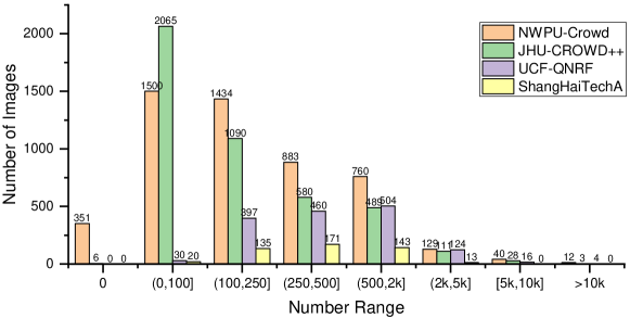
(a) The distribution of counts on the four datasets.

(b) The distribution of the area (pixels) of head region.

Figure 2: The statistical histogram of image-level counts and box-level area. The number in $x$ axis of Fig.(b) denotes $10^{x}$. For example, $[0,1]$ represents the range of box area is $[10^{0},10^{1}]$.

In addition to data volume and scale distribution, there are four more advantages in NWPU-Crowd:

1. Negative Samples. NWPU-Crowd introduces $351$ negative samples (namely nobody scenes), which are similar to congested crowd scenes in terms of texture features. It effectively improves the generalization of counting models while applied in the real world. These samples contain animal migration, fake crowd scenes (sculpture, Terra-Cotta Warriors, 2-D cartoon figure, etc.), empty hall, and other scenes with densely arranged objects that are not the person.

2. Fair Evaluation. For a fair evaluation, the labels of the test set are not public. Therefore, we develop an online evaluation benchmark website that allows researchers to submit their estimation results of the test set. The benchmark can calculate the error between presented results and ground truth, and list them on a scoreboard.

3. Higher Resolution. The proposed dataset collects high-quality and high-resolution scenes, which is entailed for extremely congested crowd counting. From Table I, the average resolution of NWPU-Crowd is $2191\times 3209$, which is larger than that of other datasets. Specifically, the maximum image size is $4028\times 19044$.

4. Large Appearance Variation. The number of people ranges from $0$ to $20,033$, which means large appearance variations within the data. Notably, the smallest head occupies only $4$ pixels, but the largest head covers $1.2\!\times\!10^{7}$ pixels. In the whole dataset, the ratio of the area of the largest and smallest head in the same image is $3.8\!\times\!10^{5}$.

In summary, NWPU-Crowd is one of the largest and most challenging crowd counting/localization datasets at present.

3.4 Data Split and Evaluation Protocol

NWPU-Crowd Dataset is randomly split into three parts, namely training, validation and test sets, which respectively contain $3,109$, $500$ and $1,500$ images. To be specific, each image is randomly assigned to a specific set with the corresponding probability (followed by $0.6$, $0.1$ and $0.3$ for the three subsets) until the number reaches the upper bound. This strategy ensures that the statistics (such as data distribution, the average value of resolutions/counts) of the subset are almost the same.

Counting Metrics     Following some previous works, we adopt three metrics to evaluate the counting performance, which are Mean Absolute Error (MAE), Mean Squared Error (MSE), and mean Normalized Absolute Error (NAE). They can be formulated as follows:

$$\tiny\begin{array}[]{l}\begin{aligned} MAE=\frac{1}{N}\sum\limits_{i=1}^{N}{\left|{{y_{i}}-{{\hat{y}}_{i}}}\right|},MSE=\sqrt{\frac{1}{N}\sum\limits_{i=1}^{N}{{{\left|{{y_{i}}-{{\hat{y}}_{i}}}\right|}^{2}}}},NAE=\frac{1}{N}\sum\limits_{i=1}^{N}{\frac{\left|{{y_{i}}-{{\hat{y}}_{i}}}\right|}{{y_{i}}}},\end{aligned}\end{array}$$ (2)

where $N$ is the number of images, ${{y_{i}}}$ is the counting label of people and ${{{\hat{y}}_{i}}}$ is the estimated value for the $i$-th test image. Since NWPU-Crowd contains quite a few negative samples, NAE’s calculation does not contain them to avoid zero denominators.

In addition to the aforementioned overall evaluation on the test set, we further assess the model from different perspectives: scene level and luminance. The former have five classes according to the number of people: $0$, $(0,100]$, $(100,500]$, $(500,5000]$, and more than $5000$. The latter have three classes based on luminance value in the YUV color space: $[0,0.25]$, $(0.25,0.5]$,and $(0.5,0.75]$. The two attribute labels are assigned to each image according to their annotated counting number and image contents. For each class in a specific perspective, MAE, MSE, and NAE are applied to the corresponding samples in the test set. Take the luminance attribute as an example, the average values of MAE, MSE, and NAE at the three categories can reflect counting models’ sensitivity to the luminance variation. Similar to the overall metrics, the negative samples are excluded during the calculation of NAE.

Localization Metrics     For the crowd localization task, we adopt the box-level Precision, Recall and F1-measure to evaluate the localization performance. Given two point sets from prediction results $P_{p}$ and ground truth $P_{g}$, we firstly construct a Bipartite Graph ${G_{p,s}}$ for the two sets. Secondly, we compute the distance matrix of $P_{p}$ and $P_{p}$. If the distance between $p_{p}\in P_{p}$ and $p_{g}\in P_{g}$ is less than the predefined distance threshold $\sigma$, we think $p_{p}$ and $p_{g}$ are successfully matched. Corresponding to each element of the distance matrix, we obtain a boolean match matrix (True and False denote matched and non-matched). Finally, we can get a Maximum Bipartite Matching for ${G_{p,s}}$ by implementing the Hungarian algorithm the match matrix and count the number of True Positive (TP), False Positive (FP) and False Negative (FN). In our evaluation, for each head with the size of width $w$ and height $h$, we define two threshold $\sigma_{s}=min(w,h)/2$ and $\sigma_{l}={\sqrt{{w^{2}}+{h^{2}}}}/2$. The former is a stricter criterion than the latter.

Similar to the category-wise counting evaluation at the image level, we propose a scale-sensitive evaluation scheme at the box level for the localization task. To be specific, all heads are divided into six categories according to their corresponding box areas: $[10^{0},10^{1}]$, $(10^{1},10^{2}]$, $(10^{2},10^{3}]$, $(10^{3},10^{4}]$, $(10^{4},10^{5}]$, and more than $10^{5}$. For each category, the Recall is calculated separately.

Different from the previous localization metrics [9, 15], the $\sigma$ in this paper is adaptive, which is defined by the real head area. In addition, the performance on different scale classes are reported, which helps researchers analyze the model more deeply. In summary, our evaluation is more reasonable than the traditional methods.

4 Experiments on Counting

In this section, we train ten mainstream open-sourced methods on the proposed NWPU-Crowd and submit their results on the evaluation benchmark. Besides, the further experimental analysis and visualization results on the validation set are discussed.

4.1 Mainstream Methods Involved in Evaluation

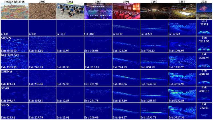
Figure 3: The eight groups of visualization results of some selected methods on the validation set.

MCNN [7]: Multi-Column Convolutional Neural Network. It is a classical and lightweight counting model, proposed by Zhang et al. in 2016. Different from the original MCNN, the RGB images are fed into the network.

SANet [33]: Scale Aggregation Network. SANet is an efficient encoder-decoder network with Instance Normalization for crowd counting, which combines the MSE loss and SSIM loss to output the high-quality density map.

PCC Net [34]: Perspective Crowd Counting Network. It is a multi-task network, which tackles the following tasks: density-level classification, head region segmentation, and density map regression. The authors provide two versions, a lightweight from scratch and VGG-16 backbone.

Reg+Det Net [35]: a subnet of DecideNet. It consists of two branches: Regression and Detection Network. The former is a light-weight network for density estimation, and the latter focuses on head detection via on Faster R-CNN (ResNet-101) [36].

C3F-VGG [37]: A simple baseline based on VGG-16 backbone for crowd counting. C3F-VGG consists of the first 10 layers of VGG-16 [31] as image feature extractor and two convolutional layers with a kernel size of 1 for regressing the density map.

CSRNet [10]: Congested Scene Recognition Network. CSRNet is a classical and efficient crowd counter, proposed by Li et al. in 2016. The authors design a Dilatation Module and add it to the top of the VGG-16 backbone. This network significantly improves performance in the field of crowd counting.

CANNet [38]: Context-Aware Network. CANNet combines the features of multiple streams using different respective field sizes. It encodes the multi-scale contextual information of the crowd scenes and yields a new record on the mainstream datasets.

SCAR [39]: Spatial-/Channel-wise Attention Regression Networks. SCAR utilizes the self-attention module [40] on the spatial and channel axis to encode the large-range contextual information. The well-designed attention models effectively extracts discriminative features and alleviates mistaken estimations.

BL [41]: Bayesian Loss for Crowd Count Estimation. Different from the traditional strategy for the generation of ground truth, BL design a loss function to directly using head point supervision. It achieves state-of-the-art performance on the UCF-QNRF dataset.

SFCN†  [20] Spatial Fully Convolutional Network with ResNet-101 [42]. SFCN†  is the only crowd counting model that uses ResNet-101 as a backbone, which shows the powerful capacity of density regression on the congested crowd scenes.

4.2 Implementation Details

In the experiments, for PCC Net and BL , the models are trained using the official codes and the default parameters. For SANet, we implement the $C^{3}$ Framework [37] and follow the corresponding parameters to train them on NWPU-Crowd dataset. For DetNet, we train a head detector using this code .

For other models, namely MCNN, RegNet, CSRNet, C3F-VGG, CANNet, SCAR, and SFCN†, they are reproduced in our counting experiments, which is developed based on $C^{3}$ Framework [37], an open-sourced crowd counting project using PyTorch [43]. In the data pre-processing stage, the high-resolution images are resized to the 2048-px scale with the original aspect ratio. The density map is generated by a Gaussian kernel with a fixed size of 15 and the $\sigma$ of 4. For augmenting the data, during the training process, all images are randomly cropped with the size of $576\times 768$, flipped horizontally, transformed to gray-scale images, and gamma corrected with a random value in $[0.4,2]$. To optimize the above counting networks, Adam algorithm [44] is employed. Other parameters (such as learning rate, batch size) are reported in https://github.com/gjy3035/NWPU-Crowd-Sample-Code.

4.3 Results Analysis on the Validation Set

Quantitative Results. Here, we list the counting performance and density quality of all participation methods in Table III. For evaluating the quality of the density map, two popular criteria are adopted, Peak Signal-to-Noise Ratio (PSNR) and Structural Similarity in Image (SSIM) [45]. Since BL [41] is supervised by point locations instead of density maps, PSNR and SSIM are not reported. In the calculation of PSNR, the negative samples are excluded to avoid zero denominators.

TABLE III: The performance of different models on the val set.

Method	the validation set
	MAE	MSE	PSNR	SSIM
MCNN	218.53	700.61	28.558	0.875
SANet	171.16	471.51	29.228	0.886
Reg+Det Net	245.8	700.3	28.862	0.751
PCC-Net-light	141.37	630.72	29.745	0.937
C3F-VGG	105.79	504.39	29.977	0.918
CSRNet	104.89	433.48	29.901	0.883
PCC-Net-VGG	100.77	573.19	30.565	0.941
CANNet	93.58	489.90	30.428	0.870
SCAR	81.57	397.92	30.356	0.920
BL	93.64	470.38	-	-
SFCN†	95.46	608.32	30.591	0.952

From the table, we find SCAR [39] attains the best counting performance, MAE of 81.57 and MSE of 397.92. SFCN†  [20] produces the most high-quality density maps, PSNR of 30.591 and SSIM of 0.952. For the three light models (MCNN, SANet, PCC-Net-light), we find that the last achieves the best SSIM (0.937), which even surpasses the SSIMs of some other VGG-based algorithms, such as C3F-VGG, CSRNet, CANNet, and SCAR. Similarly, PCC-Net-VGG is the best SSIM in the VGG-backbone methods.

Visualization Results. Fig. 3 demonstrates some predicted density maps of the eight methods. The first two columns are negative samples, and others are crowd scenes with different density levels. From the first two columns, almost all models perform poorly for negative samples, especially densely arranged objects. For humans, we can easily recognize that the two samples are mural and stones. But for the counting models, they cannot understand them. For the third column, although the predictions of these methods are good, there are still many mistaken errors in background regions. For the last two images that are extremely congested scenes, the estimation counts are far from the ground truth. SCAR is the most accurate method on the validation set, but it is about $1,900$ and $8,000$ people away from the labels, respectively. For the extreme-luminance scenes (Image 3367, 3250, and 3353), there are quite a few estimation errors in the high-light or dark-light regions. In general, the ability of the current models to cope with the above hard samples needs to be further improved.

4.4 Leaderboard

TABLE IV: The leaderboard of the counting performance on the NWPU-Crowd test set. In the ranking strategy, the Overall MAE is the primary key. “FS” represents that the model is trained From Scratch. $S0\!\sim\!S4$ respectively indicates five categories according to the different number range: $0$, $(0,100]$, …, $\geq 5000$. $L0\!\sim\!L2$ respectively denotes three luminance levels on the test set: $[0,0.25]$, $(0.25,0.5]$, and $(0.5,0.75]$. Limited by the paper length, only MAE are reported in the category-wise results. The speed and FLOPs are computed on the input size of $576\times 768$. The bold and underline fonts respectively represent the first and second place.

Method	Backbone	Overall			Scene Level (only MAE)		Luminance (only MAE)		Model Size (M)	Speed (fps)	GFLOPs
		MAE	MSE	NAE	Avg.	$S0\sim S4$	Avg.	$L0\sim L2$
MCNN	FS	232.5	714.6	1.063	1171.9	356.0/72.1/103.5/509.5/4818.2	220.9	472.9/230.1/181.6	0.133	129.0	11.867
SANet	FS	190.6	491.4	0.991	716.3	432.0/65.0/104.2/385.1/2595.4	153.8	254.2/192.3/169.7	1.389	10.8	40.195
Reg+Det Net	Hybrid	264.9	759.0	1.770	1242.5	443.0/125.5/140.5/461.5/5036.6	313.6	464.2/267.4/209.1	189.6	4.2	263.079
PCC-Net-light	FS	167.4	566.2	0.444	944.9	85.3/25.6/80.4/424.2/4108.9	141.2	253.1/167.9/144.9	0.504	12.6	72.797
C3F-VGG	VGG-16	127.0	439.6	0.411	666.9	140.9/26.5/58.0/307.1/2801.8	127.9	296.1/125.3/91.3	7.701	47.2	123.524
CSRNet	VGG-16	121.3	387.8	0.604	522.7	176.0/35.8/59.8/285.8/2055.8	112.0	232.4/121.0/95.5	16.263	26.1	182.695
PCC-Net-VGG	VGG-16	112.3	457.0	0.251	777.6	103.9/13.7/42.0/259.5/3469.1	111.0	251.3/111.0/82.6	10.207	24.0	145.157
CANNet	VGG-16	106.3	386.5	0.295	612.2	82.6/14.7/46.6/269.7/2647.0	102.1	222.1/104.9/82.3	18.103	22.0	193.580
SCAR	VGG-16	110.0	495.3	0.288	718.3	122.9/16.7/46.0/241.7/3164.3	102.3	223.7/112.7/73.9	16.287	24.5	182.856
BL	VGG-19	105.4	454.2	0.203	750.5	66.5/8.7/41.2/249.9/3386.4	115.8	293.4/102.7/68.0	21.449	34.7	182.186
SFCN†	ResNet-101	105.7	424.1	0.254	712.7	54.2/14.8/44.4/249.6/3200.5	106.8	245.9/103.4/78.8	38.597	8.8	272.763

Table IV reports the results of five methods on the test set. It lists the overall performance (MAE, MSE, and NAE), category-wise MAE on the attribute of scene level and luminance, model size, speed (inference time) and floating-point operations per second (FLOPs) . Compared with the results of the validation set, we find that the ordering has changed significantly. Although SCAR attains the best results of MAE and MSE on the validation set, the performance on the test set is not good. For the primary key (overall MAE), BL, SFCN†  and CANNet occupy the top three on the test set.

From the category-wise results of Scene Level, we find that all methods perform poorly in S0 (negative samples), S3 ($(500,5000]$) and S4 ($\geq 5000$), which causes that the average value of category-wise MAE is larger than the overall MAE (SFCN†: $712.7$ v.s. $105.7$). Besides, this phenomenon shows that negative samples and congested scenes are more challenging than sparse crowd images. Similarly, for the luminance classes, the MAE of $L0$ ($[0,0.25]$) is larger than that of $L1$ and $L2$. In other words, the counters work better under the standard luminance than under the low-luminance scenes. More detailed results are shown in https://www.crowdbenchmark.com/nwpucrowd.html.

4.5 Performance Impact between Different Scenes

From Section 4.3 and 4.4, we find that two interesting phenomena worth attention: 1) Negative samples are prone to be mistakenly estimated; 2) The data with different scene attributes (namely density level) significantly affect each other. In this section, we conduct two experiments using a simple baseline model, C3F-VGG [37], to explore the above problems.

Phenomenon 1. For the firth problem, the main reason is that the negative samples contain densely arranged objects, which is similar to the congested crowd scenes. As we all know, most existing counting models focus on texture information and local patterns for congested regions. To verify our thoughts, we design three groups of experiments to explore which samples affect the performance of negative samples. To be specific, we train three C3F-VGG counters on different combination training data: $S0+S1$, $S0+S2$, and $S0+S3+S4$ (considering that the number of S4 is small, so we integrate S3 and S4). Then the evaluation is performed on the validation set. Finally, the corresponding performance is listed in Table V. From it, the MAE on Negative Sample ($S0$) increases from $18.54$ to $147.53$ as the density of positive samples increases.

TABLE V: The MAE of the different training data on the val set.

Combination	the validation set
	$S0$	$S1$	$S2$	$S3$	$S4$
$S0+...+S4$	61.25	28.53	51.91	188.66	3730.56
$S1+...+S4$	-	33.12	68.63	238.88	3997.57
$S0+S1$	18.54	16.44	-	-	-
$S1$	-	21.00	-	-	-
$S0+S2$	64.68	-	49.97	-	-
$S2$	-	-	51.01	-	-
$S0+S3+S4$	147.53	-	-	174.49	2882.23
$S3+S4$	-	-	-	185.87	3488.25

Phenomenon 2. For the second issue, we train the counting models only using the data with a single category, $S1$, $S2$, and $S3+S4$ respectively. Removing the impacts of the negative samples, the model is trained on the data of $S1+S2+S3+S4$. The concrete performance is illustrated in Table V. According to the results, training each class individually is far better than training together. To be specific, MAE decreases by 36.6%, 25.7%, 22.2% and 12.7% on the four classes, respectively. The main reason is that NWPU-Crowd contains more diverse crowd scenes than the previous datasets. There are large appearance variations in the dataset, especially the scales of the head. At present, the existing models can not tackle this problem well.

4.6 The Effectiveness of Negative Samples

In Section 3.3, we mention that the Negative Samples (“NS” for short) can effectively improve the generalization ability of the model. Here, we conduct four groups of comparative experiments using C3F-VGG [37] to verify this opinion. To be specific, there are four types of training data: $S1$, $S2$, $S3+S4$ and $S1+...+S4$. We respectively train the models for them using NS and without NS. In other words, we add $S0$ to the above four types of training data. The concrete results are reported in Table V. After introducing NS, the category-wise MAEs are significantly reduced. Take the last six rows as the examples, the MAE is respectively decreased by 21.7%, 2.0%, 6.1% and 17.4% on the category-wise evaluation. The main reason is that NS contains diverse background objects with different structured information, which can prompt the counting models to learn more discriminative features than ever before.

4.7 Impact of Data Volume on Performance

Generally speaking, large amounts of diverse training data will prompt the model to learn more robust features, and then perform better in the wild. This is also our original intention to build a large-scale crowd counting and localization dataset. In this section, we explore the impact of different data volumes on counting performance. To be specific, we train ten C3F-VGG models using $10\%$, $20\%$, $30\%$, …, $100\%$ training data, respectively. Then evaluate them on the validation set. The performances (MAE and MSE) are demonstrated in Fig. 4. From the figure, with the gradual increase of training data, the errors on the validation set also gradually decrease overall. By comparing the MAEs when using the $10\%$ and $100\%$ data, the error is significantly reduced from 158.35 to 105.79 (relative decrease of 33.2%). Therefore, a large-scale dataset is very necessary for the community.

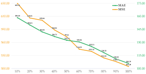
Figure 4: The results under different volumes of the training data on the validation set.

5 Experiments on Localization

Considering that the box-level labels are provided, we evaluate four crowd localization methods in this section. What’s more, we analyze the quantitative and qualitative results of them.

5.1 Methods and Implementation Details

Faster RCNN [36]: a general object detection framework, based on ResNet-101. It directly detects the head boxes, of which center is the prediction head location. We follow the original training parameters of this code . In the forward process, the thresholds of confidence and nms are set as $0.8$ and $0.3$, respectively.

TinyFaces [46]: a tiny object detection framework, which focuses on tiny faces detection. We implement the third-party code to train a detector using the default parameters. The thresholds of confidence and nms are set as $0.8$ and $0.3$, respectively.

VGG+GPR [47]: a two-stage method that consists of density map regression and point reconstruction based on Gaussian-kernel priors. C3F-VGG’s [37] training is the same as Section 4 and GPR using standard Gaussian kernel with a size of $15$.

RAZ_Loc [15]: the localization branch of RAZNet, which consists of localization map classification and point post-processing based on finding high-confidence peaks. The training details follows RAZNet, and classification threshold is set as $0.5$.

5.2 Results Analysis on the Validation Set

Table VI lists the localization and counting performance of four methods on the validation set. For each head, its $\sigma_{s}$ is less than $\sigma_{l}$, which means that the former is more strict than the latter. Thus, the localization results of $\sigma_{s}$ are worse than that of $\sigma_{l}$. From the table, we find that the Precision of Faster RCNN is better than others, but they miss quite a few objects. RAZ_Loc produces the best localization result, but its counting error is far from VGG+GPR. Detection-based methods’ counting performance is the poorest in all plans.

TABLE VI: The performance on the val set. F1-m, Pre, Rec are short for F1-measure, Precision and Recall, respectively.

Method	localization	counting
	F1-m/Pre/Rec (%)	MAE/MSE/NAE
Faster RCNN	$\sigma_{l}$:7.3/96.4/3.8	377.3/1051.2/0.798
	$\sigma_{s}$:6.8/90.0/3.5
TinyFaces	$\sigma_{l}$: 59.8/54.3/66.6	240.4/736.2/0.962
	$\sigma_{s}$: 55.3/50.2/61.7
VGG+GPR	$\sigma_{l}$: 56.3/61.0/52.2	105.8/504.4/0.931
	$\sigma_{s}$: 46.0/49.9/42.7
RAZ_Loc	$\sigma_{l}$: 62.5/69.2/56.9	128.7/665.4/0.508
	$\sigma_{s}$: 54.5/60.5/49.6

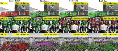
Figure 5: The three groups of qualitative localization results on the validation set. The Green point is true positive, which is inside the green circle (its center is the groundtruth position and its radius is $\sigma_{l}$); the red points and the corresponding circles are false negative; the magenta points are false positive. (For a better comparison, we transform RGB-color images to gray-scale images.)

TABLE VII: The leaderboard of the localization performance on the NWPU-Crowd test set. In the ranking strategy, the Overall F1-measure is the primary key under $\sigma_{l}$, which is bold font in Row 2 of the table. $A0\sim A4$ respectively indicates six categories according to the different head area ranges: $[10^{0},10^{1}]$, $(10^{1},10^{2}]$, $(10^{2},10^{3}]$, $(10^{3},10^{4}]$, $(10^{4},10^{5}]$, and $>10^{5}$. More detailed results will be reported in https://www.crowdbenchmark.com/nwpucrowdloc.html, which is under deployment.
*: Since the counts is transformed to integer data, the performance is slightly different from Table IV.

Method	Backbone	Training Labels		Overall ($\sigma_{l}$)		Box Level (only Rec under $\sigma_{l}$) (%)
		Point	Box	F1-m/Pre/Rec (%)	MAE/MSE/NAE	Avg.	$A0\sim A5$
Faster RCNN	ResNet-101	✗	✔	6.7/95.8/3.5	414.2/1063.7/0.791	18.2	0/0.002/0.4/7.9/37.2/63.5
TinyFaces	ResNet-101	✗	✔	56.7/52.9/61.1	272.4/764.9/0.750	59.8	4.2/22.6/59.1/90.0/93.1/89.6
VGG+GPR	VGG-16	✔	✗	52.5/55.8/49.6	127.3/439.9/0.410*	37.4	3.1/27.2/49.1/68.7/49.8/26.3
RAZ_Loc	VGG-16	✔	✗	59.8/66.6/54.3	151.5/634.7/0.305	42.4	5.1/28.2/52.0/79.7/64.3/25.1

To intuitively understand the performance of crowd localization, Fig. 5 demonstrates the visualization results of four methods on some typical samples. For the first sample, containing different-scale heads, Faster RCNN almost misses all small objects. The other three methods perform better for this scene than it. For large-scale objects (such as the second sample), Faster RCNN produces the perfect results of 100% precision and 100% recall. TinyFaces is the second, and the other two methods miss quite a few heads to different extents. In congested crowd scenes (e.g., Sample 3), VGG+GPR and RAZ_Loc obtain good results though they produce some false positives in the background regions. Faster RCNN and TinyFaces work not well for this case: the former miss 95.4% heads, and the latter yields many false positives. Besides, we also find TinyFaces produces more false positives than other methods.

In summary, there is no method to tackle the crowd localization problem well: 1) the traditional general object detection methods can not detect small-scale objects; 2) TinyFaces outputs quite a few false positives; 3) the existing regression-/classification methods can not handle large-range scale variations and mis-estimations on the background.

5.3 Leaderboard

Table VII reports the results of four methods on the test set. It lists the overall localization performance (F1-measure, Precision, and Recall) under $\sigma_{l}$ and counting performance (MAE, MSE, NAE), category-wise Recall on the different head scales (Box Level). Compared with the results of the validation set, we find that the rankings are consistent. For the primary key (overall F1-measure), RAZ_Loc attains the first place. From the category-wise results of Box Level, we find that all methods perform poorly for tiny heads (area range is $[1,10]$). The main reason is that the current feature extractor loses spatial information (usually, $8\!\times$ or $16\!\times$ downsampling are adopted). For extremely large-scale heads (area is more than $10^{5}$), detection-based methods is better than regression-/classification methods. The main reason is the latter’s label is so small (VGG+GPR: $15\!\times\!15$, RAZ_Loc: $3\!\times\!3$) that can not cover enough semantic head regions.

6 Conclusion and Outlook

In this paper, a large-scale NWPU-Crowd counting dataset is constructed, which has the characteristics of high resolution, negative samples, and large appearance variation. At the same time, we develop an online benchmark website to fairly evaluate the performance of counting models. Based on the proposed dataset, we perform the fourteen typical algorithms and rank them from the perspective of the counting and localization performance, the density map quality, and the time complexity.

According to the quantitative and qualitative results, we find some interesting phenomena and some new problems that need to be addressed on the proposed dataset:

1. How to improve the robustness of the models? In the real world, the counters may encounter many unseen data, giving incorrect estimation for background regions. Thus, the performance on negative samples is vital in the counting, which represents the models’ robustness.

2. How to remedy the performance impact between different scenes? Due to the large appearance variations, the training with all data results in an obvious performance reduction compared with the individual training for each category. Hence, it is essential to prompt the counting model’s capacity for appearance representations.

3. How to reduce the estimation errors in the extremely congested crowd scenes? Because of head occlusions, small objects, and lack of structured information, the existing models can not work well in the high-density regions.

4. How to accurately locate the tiny-size and large-scale heads together? The current detection-/regression-/classification-based methods can not handle the problem of large-range scale variation in real crowd scenes. Perhaps researchers need to design scale-aware models or hybrid methods to locate the head position accurately.

In the future, we will continue to focus on handling the above issues and dedicate to improving the performance of crowd counting and localization in the real world.

References

- [1] S. Ali and M. Shah, “A lagrangian particle dynamics approach for crowd flow segmentation and stability analysis,” in Proc. Conf. Comput. Vis. Pattern Recognit. IEEE, 2007, pp. 1–6.
- [2] S.-I. Yu, D. Meng, W. Zuo, and A. Hauptmann, “The solution path algorithm for identity-aware multi-object tracking,” in Proc. Conf. Comput. Vis. Pattern Recognit., 2016, pp. 3871–3879.
- [3] V. A. Sindagi and V. M. Patel, “Generating high-quality crowd density maps using contextual pyramid cnns,” in Proc. IEEE Int. Conf. Comput. Vis., 2017, pp. 1879–1888.
- [4] X. Liu, J. Van De Weijer, and A. D. Bagdanov, “Exploiting unlabeled data in cnns by self-supervised learning to rank,” IEEE Trans. Pattern Anal. Mach. Intell., 2019.
- [5] J. Wan, W. Luo, B. Wu, A. B. Chan, and W. Liu, “Residual regression with semantic prior for crowd counting,” in Proc. Conf. Comput. Vis. Pattern Recognit., 2019, pp. 4036–4045.
- [6] A. B. Chan, Z.-S. J. Liang, and N. Vasconcelos, “Privacy preserving crowd monitoring: Counting people without people models or tracking,” in Proc. Conf. Comput. Vis. Pattern Recognit., 2008, pp. 1–7.
- [7] Y. Zhang, D. Zhou, S. Chen, S. Gao, and Y. Ma, “Single-image crowd counting via multi-column convolutional neural network,” in Proc. Conf. Comput. Vis. Pattern Recognit., 2016, pp. 589–597.
- [8] C. Zhang, K. Kang, H. Li, X. Wang, R. Xie, and X. Yang, “Data-driven crowd understanding: a baseline for a large-scale crowd dataset,” IEEE Trans. on Multi., vol. 18, no. 6, pp. 1048–1061, 2016.
- [9] H. Idrees, M. Tayyab, K. Athrey, D. Zhang, S. Al-Maadeed, N. Rajpoot, and M. Shah, “Composition loss for counting, density map estimation and localization in dense crowds,” arXiv preprint arXiv:1808.01050, 2018.
- [10] Y. Li, X. Zhang, and D. Chen, “Csrnet: Dilated convolutional neural networks for understanding the highly congested scenes,” in Proc. Conf. Comput. Vis. Pattern Recognit., 2018, pp. 1091–1100.
- [11] V. Ranjan, H. Le, and M. Hoai, “Iterative crowd counting,” arXiv preprint arXiv:1807.09959, 2018.
- [12] L. Liu, Z. Qiu, G. Li, S. Liu, W. Ouyang, and L. Lin, “Crowd counting with deep structured scale integration network,” in Proc. IEEE Int. Conf. Comput. Vis., 2019, pp. 1774–1783.
- [13] T.-Y. Lin, M. Maire, S. Belongie, J. Hays, P. Perona, D. Ramanan, P. Dollár, and C. L. Zitnick, “Microsoft coco: Common objects in context,” in Proc. Eur. Conf. Comput. Vis., 2014, pp. 740–755.
- [14] G. Neuhold, T. Ollmann, S. Rota Bulo, and P. Kontschieder, “The mapillary vistas dataset for semantic understanding of street scenes,” in Proc. IEEE Int. Conf. Comput. Vis., 2017, pp. 4990–4999.
- [15] C. Liu, X. Weng, and Y. Mu, “Recurrent attentive zooming for joint crowd counting and precise localization,” in Proc. Conf. Comput. Vis. Pattern Recognit., 2019, pp. 1217–1226.
- [16] M. Cordts, M. Omran, S. Ramos, T. Rehfeld, M. Enzweiler, R. Benenson, U. Franke, S. Roth, and B. Schiele, “The cityscapes dataset for semantic urban scene understanding,” in Proc. Conf. Comput. Vis. Pattern Recognit., 2016, pp. 3213–3223.
- [17] K. Chen, C. C. Loy, S. Gong, and T. Xiang, “Feature mining for localised crowd counting.” in Proc. Brit. Mach. Vis. Conf., vol. 1, no. 2, 2012, p. 3.
- [18] Z. Yan, Y. Yuan, W. Zuo, X. Tan, Y. Wang, S. Wen, and E. Ding, “Perspective-guided convolution networks for crowd counting,” in Proc. IEEE Int. Conf. Comput. Vis., 2019, pp. 952–961.
- [19] H. Idrees, I. Saleemi, C. Seibert, and M. Shah, “Multi-source multi-scale counting in extremely dense crowd images,” in Proc. Conf. Comput. Vis. Pattern Recognit., 2013, pp. 2547–2554.
- [20] Q. Wang, J. Gao, W. Lin, and Y. Yuan, “Learning from synthetic data for crowd counting in the wild,” in Proc. Conf. Comput. Vis. Pattern Recognit., 2019, pp. 8198–8207.
- [21] V. A. Sindagi, R. Yasarla, and V. M. Patel, “Pushing the frontiers of unconstrained crowd counting: New dataset and benchmark method,” in Proc. IEEE Int. Conf. Comput. Vis., 2019, pp. 1221–1231.
- [22] V. Sindagi, R. Yasarla, and V. Patel, “Jhu-crowd++: Large-scale crowd counting dataset and a benchmark method,” arXiv preprint arXiv:2004.03597, 2020.
- [23] Q. Zhang and A. B. Chan, “Wide-area crowd counting via ground-plane density maps and multi-view fusion cnns,” in Proc. Conf. Comput. Vis. Pattern Recognit., 2019, pp. 8297–8306.
- [24] L. Zhang, M. Shi, and Q. Chen, “Crowd counting via scale-adaptive convolutional neural network,” in Proc. IEEE Winter Conf. Appl. Comput. Vis., 2018, pp. 1113–1121.
- [25] D. Lian, J. Li, J. Zheng, W. Luo, and S. Gao, “Density map regression guided detection network for rgb-d crowd counting and localization,” in Proc. Conf. Comput. Vis. Pattern Recognit., 2019, pp. 1821–1830.
- [26] Y. Fang, B. Zhan, W. Cai, S. Gao, and B. Hu, “Locality-constrained spatial transformer network for video crowd counting,” in Proc. IEEE Int. Conf. Multi. Expo, 2019, pp. 814–819.
- [27] W. Liu, M. Salzmann, and P. Fua, “Context-aware crowd counting,” in Proc. Conf. Comput. Vis. Pattern Recognit., 2019, pp. 5099–5108.
- [28] R. Bahmanyar, E. Vig, and P. Reinartz, “Mrcnet: Crowd counting and density map estimation in aerial and ground imagery,” arXiv preprint arXiv:1909.12743, 2019.
- [29] L. Wen, D. Du, P. Zhu, Q. Hu, Q. Wang, L. Bo, and S. Lyu, “Drone-based joint density map estimation, localization and tracking with space-time multi-scale attention network,” arXiv preprint arXiv:1912.01811, 2019.
- [30] J. Johnson, A. Alahi, and L. Fei-Fei, “Perceptual losses for real-time style transfer and super-resolution,” in Proc. Eur. Conf. Comput. Vis. Springer, 2016, pp. 694–711.
- [31] K. Simonyan and A. Zisserman, “Very deep convolutional networks for large-scale image recognition,” arXiv preprint arXiv:1409.1556, 2014.
- [32] N. R. Draper and H. Smith, Applied regression analysis. John Wiley & Sons, 1998, vol. 326.
- [33] X. Cao, Z. Wang, Y. Zhao, and F. Su, “Scale aggregation network for accurate and efficient crowd counting,” in Proc. Eur. Conf. Comput. Vis., 2018, pp. 734–750.
- [34] J. Gao, Q. Wang, and X. Li, “Pcc net: Perspective crowd counting via spatial convolutional network,” IEEE Trans. Circuits Syst. Video Technol., 2019.
- [35] J. Liu, C. Gao, D. Meng, and A. G. Hauptmann, “Decidenet: Counting varying density crowds through attention guided detection and density estimation,” in Proc. Conf. Comput. Vis. Pattern Recognit., 2018, pp. 5197–5206.
- [36] S. Ren, K. He, R. Girshick, and J. Sun, “Faster r-cnn: Towards real-time object detection with region proposal networks,” in Adv. Neural Inf. Process. Syst., 2015, pp. 91–99.
- [37] J. Gao, W. Lin, B. Zhao, D. Wang, C. Gao, and J. Wen, “C3 framework: An open-source pytorch code for crowd counting,” arXiv preprint arXiv:1907.02724, 2019.
- [38] W. Liu, M. Salzmann, and P. Fua, “Context-aware crowd counting,” in Proc. Conf. Comput. Vis. Pattern Recognit., 2019, pp. 5099–5108.
- [39] J. Gao, Q. Wang, and Y. Yuan, “Scar: Spatial-/channel-wise attention regression networks for crowd counting,” Neurocomputing, vol. 363, pp. 1–8, 2019.
- [40] X. Wang, R. Girshick, A. Gupta, and K. He, “Non-local neural networks,” in Proc. Conf. Comput. Vis. Pattern Recognit., 2018, pp. 7794–7803.
- [41] Z. Ma, X. Wei, X. Hong, and Y. Gong, “Bayesian loss for crowd count estimation with point supervision,” in Proc. IEEE Int. Conf. Comput. Vis., 2019, pp. 6142–6151.
- [42] K. He, X. Zhang, S. Ren, and J. Sun, “Deep residual learning for image recognition,” in Proc. Conf. Comput. Vis. Pattern Recognit., 2016, pp. 770–778.
- [43] A. Paszke, S. Gross, F. Massa, A. Lerer, J. Bradbury, G. Chanan, T. Killeen, Z. Lin, N. Gimelshein, L. Antiga et al., “Pytorch: An imperative style, high-performance deep learning library,” in Adv. Neural Inf. Process. Syst., 2019, pp. 8024–8035.
- [44] D. P. Kingma and J. Ba, “Adam: A method for stochastic optimization,” arXiv preprint arXiv:1412.6980, 2014.
- [45] Z. Wang, A. C. Bovik, H. R. Sheikh, and E. P. Simoncelli, “Image quality assessment: from error visibility to structural similarity,” IEEE transactions on image processing, vol. 13, no. 4, pp. 600–612, 2004.
- [46] P. Hu and D. Ramanan, “Finding tiny faces,” in Proc. Conf. Comput. Vis. Pattern Recognit., 2017, pp. 1522–1530.
- [47] J. Gao, T. Han, Q. Wang, and Y. Yuan, “Domain-adaptive crowd counting via inter-domain features segregation and gaussian-prior reconstruction,” arXiv preprint arXiv:1912.03677, 2019.