Gravitational deflection angle of light: Definition by an observer and its application to an asymptotically nonflat spacetime

Abstract

The gravitational deflection angle of light for an observer and source at finite distance from a lens object has been studied by Ishihara et al. [Phys. Rev. D, 94, 084015 (2016)], based on the Gauss-Bonnet theorem with using the optical metric. Their approach to finite-distance cases is limited within an asymptotically flat spacetime. By making several assumptions, we give an interpretation of their definition from the observer’s viewpoint: The observer assumes the direction of a hypothetical light emission at the observer position and makes a comparison between the fiducial emission direction and the direction along the real light ray. The angle between the two directions at the observer location can be interpreted as the deflection angle by Ishihara et al. The present interpretation does not require the asymptotic flatness. Motivated by this, we avoid such asymptotic regions to discuss another integral form of the deflection angle of light. This form makes it clear that the proposed deflection angle can be used not only for asymptotically flat spacetimes but also for asymptotically nonflat ones. We examine the proposed deflection angle in two models for the latter case; Kottler (Schwarzschild-de Sitter) solution in general relativity and a spherical solution in Weyl conformal gravity. Effects of finite distance on the light deflection in Weyl conformal gravity result in an extra term in the deflection angle, which may be marginally observable in a certain parameter region. On the other hand, those in Kottler spacetime are beyond reach of the current technology.

I Introduction

The gravitational deflection angle of light is of great importance in modern gravitational physics, since the pioneering experimental test of the gravitational deflection of light was done by Eddington Eddington . The gravitational deflection angle of light plays also a fundamental role in the successful observations of gravitational lensing, which enable to measure a dark matter distribution, extra solar planets and so on. Notably, the Event Horizon Telescope team has recently reported a direct imaging of the immediate vicinity of the central black hole candidate of M87 galaxy EHT .

In a conventional derivation of the gravitational deflection angle of light, a source (denoted by S) of light and an observer are assumed to be located at infinite distance from a lens object (denoted by L). Therefore, the asymptotic flatness of the spacetime is required. In the rest of this paper, the observer is called the receiver (denoted by R) in order to avoid a notational confusion between $r_{O}$ and $r_{0}$ (the closest approach) by using $r_{R}$. In astronomy, indeed, the distance from the source to the receiver is finite. Therefore, a lot of attempts have been made to discuss finite-distance effects on the gravitational deflection angle of light (e.g. Sereno ).

Gibbons and Werner proposed an alternative way of deriving the gravitational deflection angle of light GW . They also assumed that the source and receiver are located at an asymptotically Minkowskian region. They used the Gauss-Bonnet theorem GBMath to a spatial domain described by the optical metric, with which a light ray is described as a spatial curve. Their method has been largely applied to many spacetime models especially by Jusufi and his collaborators Jusufi2017a ; Jusufi2017b ; Jusufi2018 ; Crisnejo2019 .

In order to investigate finite-distance effects on the light deflection in a static and spherically symmetric spacetime, Ishihara et al. have proposed a method that extends Gibbons and Werner’s idea Ishihara2016 . This method by Ishihara et al. has been generalized to study a strong deflection case, axisymmetric spacetimes such as the Kerr solution and a rotating wormhole and also a deficit angle model Ishihara2017 ; Ono2017 ; Ono2018 ; Ono2019 . Their extensions are still limited within asymptotically flat spacetimes, because an integration range of the Gaussian curvature includes the asymptotically flat region in the space described by the optical metric.

It is interesting to extend Ishihara et al. method to a spacetime that is not asymptotically flat. The main results of this paper are two. First, by making several assumptions at the receiver location, we give an interpretation to their definition of the deflection angle. This interpretation does not require the asymptotic flatness. Secondly, motivated by this, we avoid such asymptotic regions to discuss another integral form of the deflection angle of light based on the Gauss-Bonnet theorem. Irrespective of whether the spacetime is asymptotically flat, the proposed form of the deflection angle allows us to describe finite-distance effects on the gravitational deflection angle of light.

This paper is organized as follows. In Section II, the definition of the deflection angle by Ishihara et al. is interpreted at the receiver position. We propose another form of the deflection angle based on the Gauss-Bonnet theorem, such that we can avoid treating asymptotic regions. In Section III, we examine the proposed definition of the deflection angle of light in two examples; Kottler (Schwarzschild-de Sitter) solution in general relativity and a spherical solution in Weyl conformal gravity. Finite-distance effects in these models are mentioned. Section IV is devoted to the conclusion. Throughout this paper, we use the unit of $G=c=1$.

II Avoiding the asymptotic region

II.1 The deflection angle proposed by Ishihara et al.

Following Reference Ishihara2016 , we shall briefly summarize the Ishihara et al. method and their definition. We consider a static and spherically symmetric spacetime. The metric can be written as

$$ds^{2} =g_{\mu\nu}dx^{\mu}dx^{\nu}$$

$$=-A(r)dt^{2}+B(r)dr^{2}+C(r)d\Omega^{2},$$ (1)

where $d\Omega^{2}\equiv d\theta^{2}+\sin^{2}\theta d\phi^{2}$ and $\phi$ is associated with the rotational symmetry. This metric form allows for a wormhole solution with a throat as well as a black hole spacetime. If we choose $C(r)=r^{2}$, then, $r$ denotes the circumference radius.

Ishihara et al. proposed a definition of the gravitational deflection of light, which does not require a receiver and source of light at the infinite distance from a lens object Ishihara2016 . See also Ono2019b for discussions on its observability. The definition by Ishihara et al.Ishihara2016 is

$$\alpha\equiv\Psi_{R}-\Psi_{S}+\phi_{RS},$$ (2)

where $\Psi_{S}$ and $\Psi_{R}$ are the angles between the radial direction and the light ray at the source position and at the receiver position, respectively, and $\phi_{RS}$ is a coordinate angle between the receiver and source. See Figure 1. For instance, Rindler and Ishak proposed an alternative definition of the deflection angle by their assuming that the lens, receiver and source are aligned in the Kottler spacetime Rindler ; Ishak . Their work received a lot of attention Park ; Sereno ; Bhadra ; Simpson ; Ishak2010 ; AK . Recently, Arakida made an attempt to give another definition of the deflection angle Arakida . However, he compared geodesics which belong to two different spacetimes. Therefore, it is an open issue whether his method can be mathematically justified. Motivated by Arakida’s attempt, Crisnejo, Gallo and Rogers CGR2019 proposed an alternative definition of the deflection angle, where the integration domain for the Gauss-Bonnet theorem is a finite quadrilateral. See also Figure 2 and Eq. (11) in Reference CGR2019 .

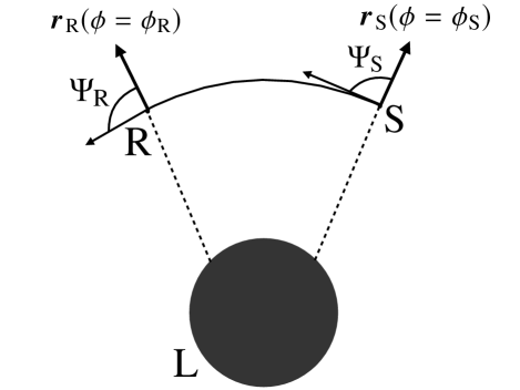
Figure 1: The light ray and radial directions. The angle between the light ray and the radial direction at the receiver is $\Psi_{R}$ and that at the source is $\Psi_{S}$. The coordinate angle between the receiver and the source is $\phi_{RS}=\phi_{R}-\phi_{S}$.

Without the loss of generality, the photon orbital plane can be chosen as the equatorial plane ($\theta=\pi/2$). By using the energy of the photon ($E$) and the angular momentum ($L$), the impact parameter of the light ray is defined as

$$b \equiv\frac{L}{E}$$

$$=\frac{C(r)}{A(r)}\frac{d\phi}{dt}.$$ (3)

By using $b$ in the null condition $ds^{2}=0$, we obtain the orbit equation as

$$\left(\frac{dr}{d\phi}\right)^{2}+\frac{C(r)}{B(r)} =\frac{\left\{C(r)\right\}^{2}}{b^{2}A(r)B(r)}.$$ (4)

$ds^{2}=0$ is solved for the time coordinate as

$$dt^{2} =\gamma_{IJ}dx^{I}dx^{J}$$

$$=\frac{B(r)}{A(r)}dr^{2}+\frac{C(r)}{A(r)}d\phi^{2},$$ (5)

where $I$ and $J$ denote $r$ and $\phi$. We refer to $\gamma_{IJ}$ as the optical metric. $\gamma_{IJ}$ defines a two-dimensional Riemannian space, in which the light ray is described as a spatial geodetic curve with $\gamma_{IJ}$ but not $g_{IJ}$. By using $\gamma_{IJ}$, the angles $\Psi_{R}$ and $\Psi_{S}$ in Eq. (2) are defined.

The Gauss-Bonnet theorem can be expressed as GBMath

$$\iint_{T}KdS+\sum_{a=1}^{N}\int_{\partial T_{a}}\kappa_{g}d\ell+\sum_{a=1}^{N}\theta_{a}=2\pi,$$ (6)

where $T$ is a two-dimensional orientable surface with boundaries $\partial T_{a}$ ($a=1,2,\cdots,N$) that are differentiable curves, $\theta_{a}$ ($a=1,2,\cdots,N$) denote jump angles, $K$ denotes the Gaussian curvature of the surface $T$, $dS$ is the area element of the surface, $\kappa_{g}$ means the geodesic curvature of $\partial T_{a}$, and $\ell$ is the line element along the boundary. See Figure 2. The sign of the line element is chosen such that it can be consistent with the surface orientation.

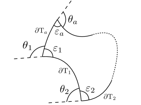
Figure 2: Schematic figure for the Gauss-Bonnet theorem. The inner angle is $\varepsilon_{a}$ and the outer (jump) angle is $\theta_{a}$.

Ishihara et al. Ishihara2016 consider a quadrilateral ${}^{\infty}_{R}\Box^{\infty}_{S}$, which consists of the spatial curve for the light ray, two outgoing radial lines from R and from S and a circular arc segment $C_{r}$ of coordinate radius $r_{C}$ ($r_{C}\to\infty$) centered at the lens which intersects the radial lines through the receiver or the source. See Figure 3. They restrict themselves within the asymptotically flat spacetime; $\kappa_{g}\to 1/r_{C}$ and $d\ell\to r_{C}d\phi$ as $r_{C}\to\infty$ (See e.g. GW ). Hence, $\int_{C_{r}}\kappa_{g}d\ell\to\phi_{RS}$. By using these things in the Gauss-Bonnet theorem for the domain ${}^{\infty}_{R}\Box^{\infty}_{S}$, we obtain

$$\alpha =\Psi_{R}-\Psi_{S}+\phi_{RS}$$

$$=-\iint_{{}^{\infty}_{R}\Box^{\infty}_{S}}KdS.$$ (7)

Eq. (7) shows that $\alpha$ is invariant in differential geometry and $\alpha$ is well-defined even if L is a singularity point, because the domain ${}^{\infty}_{R}\Box^{\infty}_{S}$ does not contain the point L. It follows that $\alpha=0$ in Euclidean space. This is because $K$ vanishes in Euclidean space and the area integral of $K$ thus vanishes.

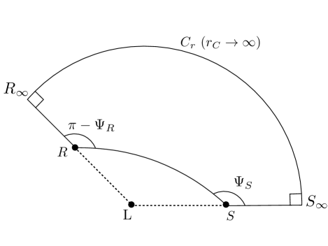
Figure 3: Quadrilateral ${}^{\infty}_{R}\Box^{\infty}_{S}$ embedded in a curved space.

II.2 Interpretation of the deflection angle of light by Ishihara et al.

Is Eq. (2) the deflection angle of light? Yes, but Ishihara et al. have not clearly discussed this issue. Therefore, we shall discuss it here.

Rigorously speaking, the parallel transport of the photon direction is done by following the null geodesic. Consequently, there is no deflection of light in the full description of the null geodesic. When we discuss the deflection of light, therefore, we have to introduce a reference direction and compare the difference between the fiducial direction and the real light ray. This procedure imitates the Eddington experiment which made, at the receiver position, a comparison between the observed (lensed) image direction and the intrinsic (unlensed) source direction.

There can be various and different definitions of such a reference direction in a general curved space. In this paper, we define a reference direction in the following manner. Where is a suitable spatial position for defining the deflection angle? From the viewpoint of observations, it would be better to choose the receiver position rather than the source position. Therefore, we allow the receiver to define the reference direction.

The angles $\Psi_{R}$ and $\Psi_{S}$ have been already defined. In principle, the receiver can measure $\Psi_{R}$ and the source can measure $\Psi_{S}$. Is $\Psi_{S}$ measured by the receiver? No for an isotropic emission of light. However, yes for an anisotropic radiation from the source in principle, as two of the present authors (Ono and Asada) argued Ono2019b . Hence, we imagine that the receiver knows the direction angle $\Psi_{S}$ of the light emission.

Let us define a reference direction at the receiver point. See Figure 4. First, we assume also that the receiver knows the relative angular position $\phi_{RS}$ between the source and receiver in the spacetime, for instance from very precise ephemeris. At the receiver, the radial direction from the lens object is denoted by $\bm{r}_{R}$. The radial direction at the source is denoted by $\bm{r}_{S}$. Instead of $\bm{r}_{S}$, the receiver defines a fiducial direction $\bm{r}_{S}^{\ast}$ by rotating the vector $\bm{r}_{R}$ with the angle $\phi_{RS}$.

If the space is Euclid, $\bm{r}_{S}^{\ast}$ equals to $\bm{r}_{S}$. This can be easily understood, when we consider, in a Euclidean space, a triangle with vertices at the lens, receiver and source and we use the parallel transport of a line. In a curved space, the receiver may use the reference direction $\bm{r}_{S}^{\ast}$ as if it were corresponding to $\bm{r}_{S}$, though $\bm{r}_{S}^{\ast}$ has no direct relation with $\bm{r}_{S}$ in a curved space.

We denote the direction of the true light ray at the receiver by $\Gamma$. Let the receiver define a fiducial direction (denoted as $\Gamma^{\ast}$) of the light emission at the receiver position. $\Gamma^{\ast}$ is defined by assuming that the angle between the reference radial direction $\bm{r}_{S}^{\ast}$ and the fiducial emission direction $\Gamma^{\ast}$ equals to $\Psi_{S}$.

The receiver can say that the deflection angle of light $\alpha$ is the angle between the light propagation direction $\Gamma$ and the fiducial emission direction $\Gamma^{\ast}$. Note that $\Gamma$ and $\Gamma^{\ast}$ are defined at the receiver position. By construction, $\alpha$ becomes $\Psi_{R}-\Psi_{S}+\phi_{RS}$. This is an interpretation of $\alpha$.

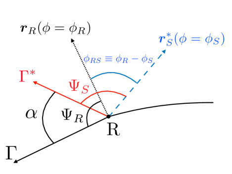
Figure 4: Angles and directions at the receiver. The (black in color) dotted line corresponds to the radial direction $\bm{r}_{R}$ at the receiver. The (black in color) solid line denotes the tangent vector $\Gamma$ to the light ray through the receiver. The (blue in color) dashed line means the fiducial radial direction $\bm{r}_{S}^{\ast}$ that is assumed by the receiver. The (red in color) solid line is the hypothetical emission direction $\Gamma^{\ast}$ that is defined by the receiver. The angle between the radial direction $\bm{r}_{R}$ and the light ray $\Gamma$ is denoted as $\Psi_{R}$. The receiver defines the fiducial radial direction $\bm{r}_{S}^{\ast}$, such that the angle between $\bm{r}_{R}$ and $\bm{r}_{S}^{\ast}$ can be the same as $\phi_{RS}$. The receiver defines also the hypothetical emission direction $\Gamma^{\ast}$, such that the angle between $\Gamma^{\ast}$ and $\bm{r}_{S}^{\ast}$ can be the same as $\Psi_{S}$. As a result, the angle between the light ray $\Gamma$ and the hypothetical emission direction $\Gamma^{\ast}$ is $\Psi_{R}-\Psi_{S}+\phi_{RS}$.

II.3 Another integral form of the deflection angle of light

The above interpretation of the deflection angle does not require the asymptotic flatness, while the integral in Eq. (7) needs $r\to\infty$. This motivates us to reexamine Eq. (7). We consider the following region that is defined by using the receiver, source and the closest approach of the light ray. See Figure 5 for this domain. The boundaries of this region are the radial lines through $R$ or $S$, the light ray from $S$ to $R$, and the circle arc segment $C_{0}$ with radius of the closest approach $r_{0}$. This domain is divided into two trilaterals. We denote one trilateral containing the receiver point by $D_{R}$ and the other trilateral containing the source point by $D_{S}$. In both of them, the inner angle at the closest approach is zero, because the radial coordinate $r$ in a light ray has a minimum at the closest approach.

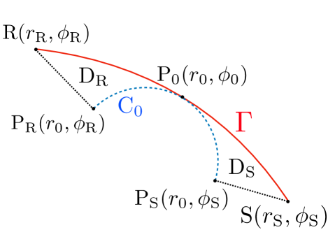
Figure 5: $D_{R}$ and $D_{S}$. $D_{R}$ is a trilateral specified by the points $R$, $P_{0}$ and $P_{R}$. $D_{S}$ is that specified by the points $S$, $P_{0}$ and $P_{S}$.

For the domain $D_{R}$ in Figure 5, we use the Gauss-Bonnet theorem to obtain

$$\iint_{D_{R}}KdS+\int_{P_{R}}^{P_{0}}\kappa_{g}d\ell-\Psi_{R}+\frac{\pi}{2}=0,$$ (8)

where $P_{0}$ denotes the periastron (the closest approach). In the similar manner for $D_{S}$, we obtain

$$\iint_{D_{S}}KdS+\int_{P_{0}}^{P_{S}}\kappa_{g}d\ell+\Psi_{S}-\frac{\pi}{2}=0.$$ (9)

By combining Eqs. (8) and (9), we find

$$\Psi_{R}-\Psi_{S}=\iint_{D_{R}+D_{S}}KdS+\int_{P_{R}}^{P_{S}}\kappa_{g}d\ell.$$ (10)

Hence, $\alpha$ in Eq. (2) is rewritten as

$$\alpha=\iint_{D_{R}+D_{S}}KdS+\int_{P_{R}}^{P_{S}}\kappa_{g}d\ell+\phi_{RS}.$$ (11)

The right-hand side of this equation contains the radial coordinate $r\in[r_{0},r_{R}]$ or $[r_{0},r_{S}]$. Indeed, this radial interval is exactly the same as that for the light ray from the source to the receiver. On the other hand, the integration range for the radial coordinate in Ishihara et al. is $r\in[r_{0},\infty]$ . Therefore, they needed the asymptotic flatness for treating $r\sim\infty$. The new form of $\alpha$ by Eq. (11) is better than the previous form by Eq. (7), in the sense that Eq. (11) does not require the asymptotic flatness. Note that neither Eq. (7) nor Eq. (11) needs any constraint on the lens point L. Namely, the lens object in the present method can be a black hole with a horizon or a wormhole with a throat.

Please see the next section for Eq. (11) in asymptotically nonflat spacetime models.

III Examples in asymptotically nonflat spacetimes

III.1 Kottler spacetime

As a first example of asymptotically nonflat spacetimes, we consider the Kottler solution Kottler . The line element is

$$ds^{2}= -\left(1-\frac{r_{g}}{r}-\frac{\Lambda}{3}r^{2}\right)dt^{2}+\left(1-\frac{r_{g}}{r}-\frac{\Lambda}{3}r^{2}\right)^{-1}dr^{2}$$

$$+r^{2}(d\theta^{2}+\sin^{2}\theta d\phi^{2}),$$ (12)

where $r_{g}$ and $\Lambda$ are constants. For this spacetime, the optical metric on the equatorial plane ($\theta=\pi/2$) becomes

$$\gamma_{rr} =\left(1-\frac{r_{g}}{r}-\frac{\Lambda}{3}r^{2}\right)^{-2},$$ (13)

$$\gamma_{\phi\phi} =r^{2}\left(1-\frac{r_{g}}{r}-\frac{\Lambda}{3}r^{2}\right)^{-1}.$$ (14)

In the following, we use the linear approximations in $r_{g}$ and $\Lambda$. We thus neglect $O(r_{g}^{2})$ and $O(\Lambda^{2})$.

The Gaussian curvature is calculated as

$$K =\frac{R_{r\phi r\phi}}{\det(\gamma_{IJ})}$$

$$=-\frac{r_{g}}{r^{3}}+\frac{r_{g}\Lambda}{r}-\frac{\Lambda}{3}+O\left(r^{2}_{g},\Lambda^{2}\right),$$ (15)

where the Riemann tensor is calculated by using $\gamma_{IJ}$. The area element on the equatorial plane is

$$dS =\sqrt{\det(\gamma_{IJ})}drd\phi$$

$$=r\left(1-\frac{r_{g}}{r}-\frac{\Lambda}{3}r^{2}\right)^{-\frac{3}{2}}drd\phi.$$ (16)

We define $u$ as the inverse of $r$. The photon orbit equation is written as

$$\left(\frac{du}{d\phi}\right)^{2}=\frac{1}{b^{2}}-u^{2}+r_{g}u^{3}+\frac{\Lambda}{3}.$$ (17)

The iterative solution is obtained as

$$u= \frac{\sin\phi}{b}+\frac{r_{g}}{2b^{2}}(1+\cos^{2}\phi)$$

$$+\frac{b\Lambda}{6}\sin\phi+\frac{r_{g}\Lambda}{6}(1+\cos^{2}\phi)+O(r^{2}_{g},\Lambda^{2}).$$ (18)

By using the above equations, we obtain

$$\int_{D_{R}+D_{S}}KdS= \frac{r_{g}}{b}\left(\sqrt{1-b^{2}u^{2}_{S}}+\sqrt{1-b^{2}u^{2}_{R}}\right)$$

$$-\frac{b\Lambda}{6}\left(\frac{\sqrt{1-b^{2}u^{2}_{S}}}{u_{S}}+\frac{\sqrt{1-b^{2}u^{2}_{R}}}{u_{R}}\right)$$

$$+\frac{r_{g}b\Lambda}{12}\left(\frac{1}{\sqrt{1-b^{2}u^{2}_{S}}}+\frac{1}{\sqrt{1-b^{2}u^{2}_{R}}}\right)$$

$$+\left(\frac{b^{2}\Lambda}{6}-\frac{r_{g}}{b}-\frac{r_{g}}{3}b\Lambda\right)\phi_{RS}$$

$$+O(r^{2}_{g},\Lambda^{2}).$$ (19)

The geodesic curvature along a line is Ono2017

$$\kappa_{g} =\epsilon_{ijk}N^{i}A^{j}T^{k},$$ (20)

where $\epsilon_{ijk}$ is the Levi-Civita tensor, $N_{i}$ denotes the unit normal vector to the surface, $A^{j}$ is the acceleration vector of the line, and $T^{k}$ means the unit tangent vector along the line. For the circle arc segment with radius $r_{0}$, $A^{j}$ is the acceleration vector of the arc segment, and $T^{k}$ is the unit tangent vector along the arc. The exact form of the geodesic curvature becomes

$$\kappa_{g} =\frac{1}{r^{2}_{0}}\left(r_{0}-\frac{3}{2}r_{g}\right).$$ (21)

$$\int^{P_{S}}_{P_{R}}\kappa_{g}d\ell= -\phi_{RS}+\frac{r_{g}}{b}\phi_{RS}+\frac{r_{g}b\Lambda}{3}\phi_{RS}-\frac{b^{2}\Lambda}{6}\phi_{RS}$$

$$+O\left(r^{2}_{g},\Lambda^{2}\right).$$ (22)

Combining Eqs. (19) and (22) leads to the deflection angle as

$$\alpha_{Kottler}= \frac{r_{g}}{b}\left(\sqrt{1-b^{2}u^{2}_{S}}+\sqrt{1-b^{2}u^{2}_{R}}\right)$$

$$-\frac{b\Lambda}{6}\left(\frac{\sqrt{1-b^{2}u^{2}_{S}}}{u_{S}}+\frac{\sqrt{1-b^{2}u^{2}_{R}}}{u_{R}}\right)$$

$$+\frac{r_{g}b\Lambda}{12}\left(\frac{1}{\sqrt{1-b^{2}u^{2}_{S}}}+\frac{1}{\sqrt{1-b^{2}u^{2}_{R}}}\right)$$

$$+O\left(r^{2}_{g},\Lambda^{2}\right),$$ (23)

where the leading order terms in $\phi_{RS}$ cancel out. Eq. (23) fully agrees with Eq. (37) in Ishihara et al. (2016) Ishihara2016 . Note that Ishihara et al. (2016) obtained this equation by using the form of $\Psi_{R}-\Psi_{S}+\phi_{RS}$ but not by using their integral form as $\int_{{}^{\infty}_{R}\Box^{\infty}_{S}}KdS$. Note that their integral diverges. This divergent behavior is merely because the integral in Ishihara (2016) is ill-defined for the asymptotically nonflat cases. In Kottler spacetime, $K$ diverges as $r\to\infty$.

We briefly discuss how the finite distance affects the light deflection in Kottler spacetime. For the simplicity, we assume $u_{R}=u_{S}\equiv U$ and focus on the coupling between the mass and the cosmological constant. A function $V(U)$ for this coupling is defined as the third line of Eq. (23)

$$V(U)\equiv\frac{r_{g}b\Lambda}{6\sqrt{1-b^{2}U^{2}}}.$$ (24)

Please see Figure 6 for the difference as $V(U)-V(0)$. Note that Kottler solution does not allow $r\to\infty$ ($U\to 0$) but $V(U)$ is finite as $r\to\infty$. This figure shows how the light deflection at finite-distance receiver and source differs from that when the receiver and source are at infinity. In this figure, we assume that the lens mass is $m\sim 10^{15}M_{\odot}$ (as a cluster of galaxies), $\Lambda=(r_{H})^{-2}\sim 10^{-52}\mbox{m}^{-2}$, and $b=1$ Mpc, where $r_{H}$ denotes the Hubble horizon radius $\sim 10$ Gpc. The largest difference of $V(U)-V(0)$ is $\sim 10^{-3}$ microarcseconds for $r_{R}=r_{S}\sim b$. Even the largest difference is thus beyond reach of the current technology. Here, we ignore the pure de-Sitter term (the second line) in Eq. (23) for the deflection angle in the Kottler model. This term does not make any sense at infinity ($r_{R},r_{S}\to\infty$) and indeed it diverges there. However, we should note that the coupling part between $r_{g}$ and $\Lambda$ (the third line) in Eq. (23) remains finite at infinity, though it may make no physical meaning there. For readers’ convenience, we rearrange only the coupling part in Eq. (23) as

$$\frac{r_{g}b\Lambda}{12}\left(\frac{1}{\sqrt{1-b^{2}u^{2}_{S}}}+\frac{1}{\sqrt{1-b^{2}u^{2}_{R}}}\right)$$

$$=\frac{r_{g}b\Lambda}{6}+\frac{r_{g}b\Lambda}{12}\left(\frac{1}{\sqrt{1-b^{2}u^{2}_{S}}}+\frac{1}{\sqrt{1-b^{2}u^{2}_{R}}}-2\right),$$ (25)

where the first term in the second line is the deflection at infinity and the second term denotes the finite-distance effect.

We mention also M87^∗, the central black hole candidate of M87. The finite $r_{S}$ is fully taken into account in general relativistic simulations around the black hole. Therefore, we consider finite distance to the receiver in this paragraph. We focus on the coupling term containing $r_{R}$, $r_{g}$ and $\Lambda$, which is expressed by the second term in the third line of Eq. (23). This term is $\sim 10^{-26}$ where we assume $r_{R}\sim 16\mbox{Mpc}\sim 10^{23}\mbox{m}$, $r_{g}\sim 7\times 10^{9}M_{\odot}\sim 10^{13}\mbox{m}$, $b\sim 10r_{g}\sim 10^{14}\mbox{m}$, $\Lambda\sim 10^{-52}\mbox{m}^{-2}$. Therefore, the effect by finite $r_{R}$ in Kottler model can be safely ignored also for M87^∗.

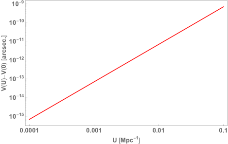
Figure 6: Effects of the finite distance on the deflection of light in Kottler spacetime. The vertical axis denotes the difference $V(U)-V(0)$, where $u_{R}=u_{S}=U$ and $V(U)$ is defined by Eq. (24). The horizontal axis is $U$, for which we consider a range as $\sqrt{\Lambda}<U<(10b)^{-1}$. Here, we assume that the lens is a cluster of galaxies with mass $10^{15}M_{\odot}$, $\Lambda=(10\mbox{Gpc})^{-2}$, and $b=1$ Mpc for the simplicity. The values of $U$ to 0.1 - 1000 $\mbox{Mpc}{}^{-1}$ mean that the receiver and source are located within 10Mpc - 1kpc from the lens. This situation is not realistic in astronomy. Therefore, we do not consider these values of $U$ in this plot.

III.2 Spherical solution in Weyl gravity

For the next example, we consider a static and spherically symmetric solution in the conformal Weyl gravity MK . The metric for this solution is

$$ds^{2}=-B(r)dt^{2}+B^{-1}(r)dr^{2}+r^{2}(d\theta^{2}+\sin^{2}\theta d\phi^{2}).$$ (26)

Here, we assume $m\ll 1/\gamma$. Namely, $m\gamma\ll 1$. Therefore, we can neglect $m^{2}\gamma(=m\times m\gamma\ll m)$. $B(r)$ can be approximated as

$$B(r)=1-3m\gamma-\frac{2m}{r}+\gamma r-kr^{2}.$$ (27)

For the conformal Weyl gravity, Birkoff’s theorem was proven Riegert . Several authors made attempts to calculate the deflection angle in this spacetime Edery ; Pireaux2004a ; Pireaux2004b ; Sultana ; Cattani ; Ishihara2016 .

In the Kottler spacetime, we have studied the squared-$r$ term in the metric. For simplifying our analysis, we neglect $k$ to choose $k=0$.

For this spacetime, the optical metric on the equatorial plane ($\theta=\pi/2$) becomes

$$\gamma_{rr} =[B(r)]^{-2},$$ (28)

$$\gamma_{\phi\phi} =r^{2}[B(r)]^{-1}.$$ (29)

In the following, we consider the small deflection and weak field approximations. Namely, $m\ll b\ll r_{R},r_{S}$ and $r_{R},r_{S}\ll 1/\gamma$. We focus on the linear-order effects by $\gamma$. Hence, we neglect $O(\gamma^{2})$.

The Gaussian curvature is calculated as

$$K= -\frac{2m}{r^{3}}-\frac{3m\gamma}{r^{2}}+O\left(m^{2},\gamma^{2}\right),$$ (30)

where the Riemann tensor is calculated by using $\gamma_{IJ}$. The area element on the equatorial plane is

$$dS =\sqrt{\det(\gamma_{IJ})}drd\phi$$

$$=r[B(r)]^{-\frac{3}{2}}drd\phi.$$ (31)

The photon orbit equation becomes

$$\left(\frac{du}{d\phi}\right)^{2}=\frac{1}{b^{2}}-u^{2}+2mu^{3}+3m\gamma u^{2}-\gamma u.$$ (32)

The iterative solution is obtained as

$$u= \frac{\sin\phi}{b}+\frac{m}{b^{2}}(1+\cos^{2}\phi)-\frac{\gamma}{2}+O(m^{2},\gamma^{2}),$$ (33)

where terms at $O(m\gamma)$ do not appear.

By using the above equations, we obtain

$$\int_{D_{R}+D_{S}}KdS= \frac{2m}{b}\left(\sqrt{1-b^{2}u^{2}_{S}}+\sqrt{1-b^{2}u^{2}_{R}}\right)$$

$$-m\gamma\left(\frac{bu_{S}}{\sqrt{1-b^{2}u^{2}_{S}}}+\frac{bu_{R}}{\sqrt{1-b^{2}u^{2}_{R}}}\right)$$

$$-\frac{2m}{b}\phi_{RS}$$

$$+O(m^{2},\gamma^{2}).$$ (34)

The exact form of the geodesic curvature is calculated as

$$\kappa_{g}= \frac{1}{r_{0}}\left(1-\frac{3m}{r_{0}}-3m\gamma+\frac{\gamma}{2}r_{0}\right).$$ (35)

The integral of the geodesic curvature is

$$\int^{P_{S}}_{P_{R}}\kappa_{g}d\ell= -\phi_{RS}+\frac{2m}{b}\phi_{RS}+O\left(m^{2},\gamma^{2}\right).$$ (36)

Combining Eqs. (34) and (36) leads to the deflection angle as

$$\alpha_{Weyl}= \frac{2m}{b}\left(\sqrt{1-b^{2}u^{2}_{S}}+\sqrt{1-b^{2}u^{2}_{R}}\right)$$

$$-m\gamma\left(\frac{bu_{S}}{\sqrt{1-b^{2}u^{2}_{S}}}+\frac{bu_{R}}{\sqrt{1-b^{2}u^{2}_{R}}}\right)$$

$$+O\left(m^{2},\gamma^{2}\right),$$ (37)

where terms at $O(\gamma)$ do not appear. Eq. (37) coincides with Eq. (42) in Ishihara et al. (2016) Ishihara2016 . Note that Ishihara et al. (2016) obtained the same equation through $\Psi_{R}-\Psi_{S}+\phi_{RS}$ but not the integral form as $\int_{{}^{\infty}_{R}\Box^{\infty}_{S}}KdS$. Note that this integral diverges. This divergent behavior is merely because the integral domain in Ishihara (2016) is ill-defined for the asymptotically nonflat cases. For the spherical model in Weyl gravity, $K$ remains finite but its area integral diverges as $r\to\infty$ Ishihara2016 .

Note that the $m\gamma$ coupling term in Eq. (37) vanishes in the limit as $r_{R},r_{S}\to\infty$. Therefore, this coupling term does not appear in the literature Pireaux2004a ; Pireaux2004b ; Sultana ; Cattani before Reference Ishihara2016 . Ishihara et al. (2016) Ishihara2016 suggests the existence of this term. However, their integral diverges and hence it has been an open issue whether this term exists. By using the well-defined integral, the present paper confirms that the $m\gamma$-coupling term results from the finite distance.

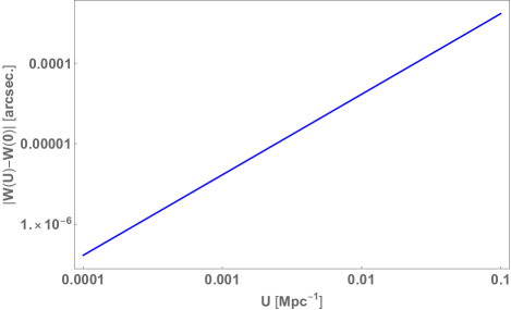
Figure 7: Effects of the finite distance on the deflection of light in Weyl gravity. The vertical axis denotes the difference $|W(U)-W(0)|$, where $u_{R}=u_{S}=U$ and $W(U)$ is defined by Eq. (38). The horizontal axis is $U$, for which we consider a range as $\gamma<U<(10b)^{-1}$. Here, we assume that the lens mass is $10^{15}M_{\odot}$, $\gamma=(10\mbox{Gpc})^{-1}$, and $b=1$ Mpc for the simplicity.

Finally, we discuss how the finite distance affects the light deflection for the spherical model in Weyl gravity. We assume $u_{R}=u_{S}\equiv U$ and focus on the coupling between the mass and the $\gamma$ parameter. A function $W(U)$ due to this coupling is defined by the second line of Eq. (37) as

$$W(U)\equiv-2m\gamma\frac{bU}{\sqrt{1-b^{2}U^{2}}}.$$ (38)

$W(U)$ is negative if $\gamma>0$. This means that this term is a negative correction to the deflection angle if $\gamma$ is positive.

Please see Figure 7 for the difference as $|W(U)-W(0)|$, where $W(0)=0$. This figure shows how the light deflection at finite-distance receiver and source differs from that when the receiver and source are at infinity. In this figure, we assume that the lens mass is $10^{15}M_{\odot}$, $\gamma=(r_{H})^{-1}$, and $b=1$ Mpc. The largest difference of $|W(U)-W(0)|$ is $\sim O(10^{2})$ microarcseconds, if $r_{R}\sim r_{S}\sim 10\times b$. This effect as $\sim O(10^{2})$ microarcseconds is marginally within the current VLBI accuracy. Therefore, the Weyl gravity model in the parameter region $\gamma\sim(r_{H})^{-1}$ may be relevant with the current observation. However, Eddington-type measurements (which use the source and Earth motion and make a comparison between a lensed image position and an unlensed position) cannot be used for a light source such as a quasar at cosmological distance. Further investigations of how to test the $m\gamma$ coupling term in Weyl gravity by lensing observations at cosmological distance are left for future.

Interestingly, effects of finite distance in Weyl gravity may be relevant to the current observation, though those in Kottler are negligible as discussed in Section III.A. Why does such a crucial difference occur? The reason is the dependence on $r_{H}$. For the simplicity, we assume that $bU$ is small but not so negligible, for instance $bU\sim 1/10$. Eq. (24) is roughly approximated as

$$V(U)\sim\frac{1}{6}\left(\frac{r_{g}}{r_{H}}\right)^{2}\left(\frac{b}{r_{g}}\right),$$ (39)

where $\Lambda\sim(r_{H})^{-2}$ and we neglected $b^{2}U^{2}\sim 10^{-2}$ . On the other hand, Eq. (38) is roughly approximated as

$$W(U)\sim-\frac{1}{5}\left(\frac{m}{r_{H}}\right)\left(\frac{bU}{1/10}\right),$$ (40)

where $\gamma\sim(r_{H})^{-1}$. $V(U)$ is significantly suppressed by the inverse square of $r_{H}$ and thus it is negligible, while $W(U)$ is proportional to the inverse of $r_{H}$ and thus it is mildly small but not so negligible.

For readers’ convenience, we rearrange Eq. (37) as

$$\alpha_{Weyl}=\alpha_{Weyl}^{\infty}+\alpha_{Weyl}^{F},$$ (41)

where $\alpha_{Weyl}^{\infty}$ is $\alpha_{Weyl}$ at infinity ($r_{R},r_{S}\to\infty$) and $\alpha_{Weyl}^{F}$ denotes the finite-distance effect on the light deflection.

$$\alpha_{Weyl}^{\infty}= \frac{4m}{b}+O\left(m^{2},\gamma^{2}\right).$$ (42)

$$\alpha_{Weyl}^{F}= \frac{2m}{b}\left(\sqrt{1-b^{2}u^{2}_{S}}+\sqrt{1-b^{2}u^{2}_{R}}-2\right)$$

$$-m\gamma\left(\frac{bu_{S}}{\sqrt{1-b^{2}u^{2}_{S}}}+\frac{bu_{R}}{\sqrt{1-b^{2}u^{2}_{R}}}\right)$$

$$+O\left(m^{2},\gamma^{2}\right).$$ (43)

IV Conclusion

From the receiver’s viewpoint, we made an attempt to provide a physical interpretation of the deflection angle defined by Ishihara et al. Ishihara2016 . This interpretation does not need the asymptotic flatness. Therefore, this interpretation encouraged us to seek another integral form of the deflection angle of light. The proposed integral form of the deflection angle can be used not only for asymptotically flat spacetimes but also for asymptotically nonflat ones. By doing explicit calculations, we examined the proposed deflection angle in two asymptotically nonflat spacetime models; the Kottler solution and a spherical solution in Weyl conformal gravity.

According to the present order-of-magnitude estimate, the extra deflection angle in Weyl gravity is within accuracy of the current VLBI, if some parameter values are in a certain range. Further investigations of how to test Weyl gravity by lensing observations are needed. On the other hand, effects of finite distance in Kottler spacetime can be safely ignored.

Extensions to a case without spherical symmetry and so on are left for future.

- (1) F. W. Dyson, A. S. Eddington, and C. Davidson, Phil. Trans. R. Soc. A 220, 291 (1920).
- (2) K. Akiyama et al. (Event Horizon Telescope Collaboration), Astrophys. J. 875, L1 (2019); Astrophys. J. 875, L2 (2019); Astrophys. J. 875, L3 (2019); Astrophys. J. 875, L4 (2019); Astrophys. J. 875, L5 (2019); Astrophys. J. 875, L6 (2019).
- (3) M. Sereno, Phys. Rev. Lett. 102, 021301 (2009).
- (4) G. W. Gibbons and M. C. Werner, Class. Quantum Grav. 25, 235009 (2008).
- (5) M. P. Do Carmo, Differential Geometry of Curves and Surfaces, pages 268-269, (Prentice-Hall, New Jersey, 1976).
- (6) K. Jusufi, M. C. Werner, A. Banerjee, and A. Ovgun, Phys. Rev. D 95, 104012 (2017).
- (7) K. Jusufi, A. Ovgun, and A. Banerjee Phys. Rev. D 96, 084036 (2017).
- (8) K. Jusufi, and A. Ovgun, Phys. Rev. D 97, 024042, (2018).
- (9) G. Crisnejo, E. Gallo, and K. Jusufi, Phys. Rev. D 100, 104045 (2019)
- (10) A. Ishihara, Y. Suzuki, T. Ono, T. Kitamura and H. Asada, Phys. Rev. D 94, 084015 (2016).
- (11) A. Ishihara, Y. Suzuki, T. Ono and H. Asada, Phys. Rev. D 95, 044017 (2017).
- (12) T. Ono, A. Ishihara, and H. Asada, Phys. Rev. D 96, 104037 (2017).
- (13) T. Ono, A. Ishihara, and H. Asada, Phys. Rev. D 98, 044047 (2018).
- (14) T. Ono, A. Ishihara, and H. Asada, Phys. Rev. D 99, 124030 (2019).
- (15) T. Ono, and H. Asada, Universe, 5(11), 218 (2019).
- (16) W. Rindler and M. Ishak, Phys. Rev. D 76, 043006 (2007).
- (17) M. Ishak and W. Rindler, Gen. Relativ. Gravit. 42, 2247 (2010).
- (18) M. Park, Phys. Rev. D 78, 023014 (2008).
- (19) A. Bhadra, S. Biswas, and K. Sarkar, Phys. Rev. D 82, 063003 (2010).
- (20) F. Simpson, J. A. Peacock, and A. F. Heavens, Mon. Not. R. Astron. Soc. 402, 2009 (2010).
- (21) M. Ishak,W. Rindler and J. Dossett, Mon. Not. Roy. Astron. Soc. 403, 2152 (2010).
- (22) H. Arakida, and M. Kasai, Phys. Rev. D 85, 023006 (2012).
- (23) H. Arakida, Gen. Rel. Grav. 50, 48 (2018).
- (24) G. Crisnejo, E. Gallo, and A. Rogers, Phys. Rev. D 99, 124001 (2019).
- (25) F. Kottler, Annalen. Phys. 361, 401 (1918).
- (26) P. D. Mannheim and D. Kazanas, Astrophys. J. 342, 635 (1989).
- (27) R. J. Riegert, Phys. Rev. Lett. 53, 315 (1984).
- (28) A. Edery, and M. B. Paranjape, Phys. Rev. D 58, 024011 (1998).
- (29) S. Pireaux, Classsical Quantum Gravity, 21, 1897 (2004).
- (30) S. Pireaux, Classical Quantum Gravity, 21, 4317 (2004).
- (31) J. Sultana, and D. Kazanas, Phys. Rev. D 81, 127502 (2010).
- (32) C. Cattani, M. Scalia, E. Laserra, I. Bochicchio, and K. K. Nandi, Phys. Rev. D 87, 047503 (2013).