Abstract

While deep neural net inference was considered a task for servers only, latest advances in technology allow the task of inference to be moved to mobile and embedded devices, desired for various reasons ranging from latency to privacy. These devices are not only limited by their compute power and battery, but also by their inferior physical memory and cache, and thus, an efficient memory manager becomes a crucial component for deep neural net inference at the edge. We explore various strategies to smartly share memory buffers among intermediate tensors in deep neural nets. Employing these can result in up to 11% smaller memory footprint than the state of the art.

1 Introduction

Deep neural networks are widely used to solve various machine learning problems including, but not limited to, computer vision, natural language processing, signal processing, and others. While employing deep neural networks is technically challenging for its demanding resources in computation and memory, recent advances in computing hardware enabled deep neural nets to be carried out on mobile and embedded devices Lee et al. (2019); Wu et al. (2019).

Deep neural networks can be represented as directed acyclic graphs (DAG) with the nodes describing the computational operations such as convolution or softmax and the edges describing the tensors containing the intermediate computation results between the operators Bergstra et al. (2010). These tensors are materialized with memory buffers: A tensor of shape $[B,H,W,C]$ translates to a memory buffer of size ${B}\times{H}\times{W}\times{C}\times\textrm{sizeof(float)}$. To reduce the overhead of dynamic memory allocation, the memory buffers for intermediate tensors are typically allocated before running the model, but these can take up a significant amount of memory. For example, the intermediate tensors of Inception v3 Szegedy et al. (2016) take up 37% of $147\text{\,}\mathrm{MB}$ total run-time memory and those of MobileNet v2 Sandler et al. (2018) consume 63% of $41\text{\,}\mathrm{MB}$.

Fortunately, the intermediate tensors do not have to co-exist in memory; thanks to the mostly sequential execution of the network due to data dependency, only one operator is active at any given point in time, and only its immediate input and output intermediate tensors are needed. Thus, we explore the idea of reusing the memory buffers to optimize the total memory footprint of the deep neural net inference engine. If the DAG has the shape of a simple chain, memory buffers can be reused in alternating fashion, assuming the memory buffers have enough capacity to contain any intermediate tensor in the network. However, the reusing problem is not trivial to solve if memory buffers have limited capacity or the network contains residual connections He et al. (2016).

In this paper, we present five strategies for efficient memory sharing for intermediate tensors. They show up to $10.5\times$ reduction compared to keeping all of the intermediate tensors naïvely in memory and up to 11% reduction of memory consumption compared to prior state of the art. Efficiently reusing memory buffers leads to improved cache hit rate that can also translate to up to 10% improvement in inference speed. These strategies are applicable to neural net inference only and not to training as intermediate tensors need to be kept alive and thus their memory cannot be re-purposed.

2 Related Work

Efficiently managing memory for deep neural networks is not only a problem for resource-constrained environment but also for servers. MXNet employs a number of techniques for reducing memory consumption such as in-place operators and intermediate tensors memory co-share, using simple heuristic algorithm for memory allocation, that is safe for parallel operators execution Chen et al. (2015). However, the authors do not focus on the core problem of memory management and do not explore different algorithms that can solve this problem in the most effective way. Chen et al. (2016) employs a similar technique along with trading computation for memory, but is not suitable for mobile.

Caffe2’s on-device inference engine employs NNPACK and QNNPACK Wu et al. (2019). These neural network operator libraries choose the best data layout and optimize off-chip memory access, but do not focus on minimizing the inference engine’s memory footprint. Li et al. (2016) similarly exploits data layout to optimize off-chip memory access and focuses on server-like settings which are not as resource-constrained as mobile or embedded devices.

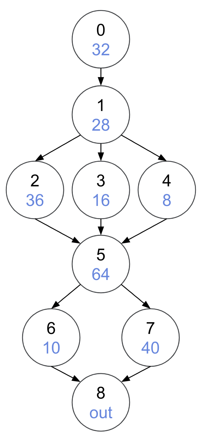
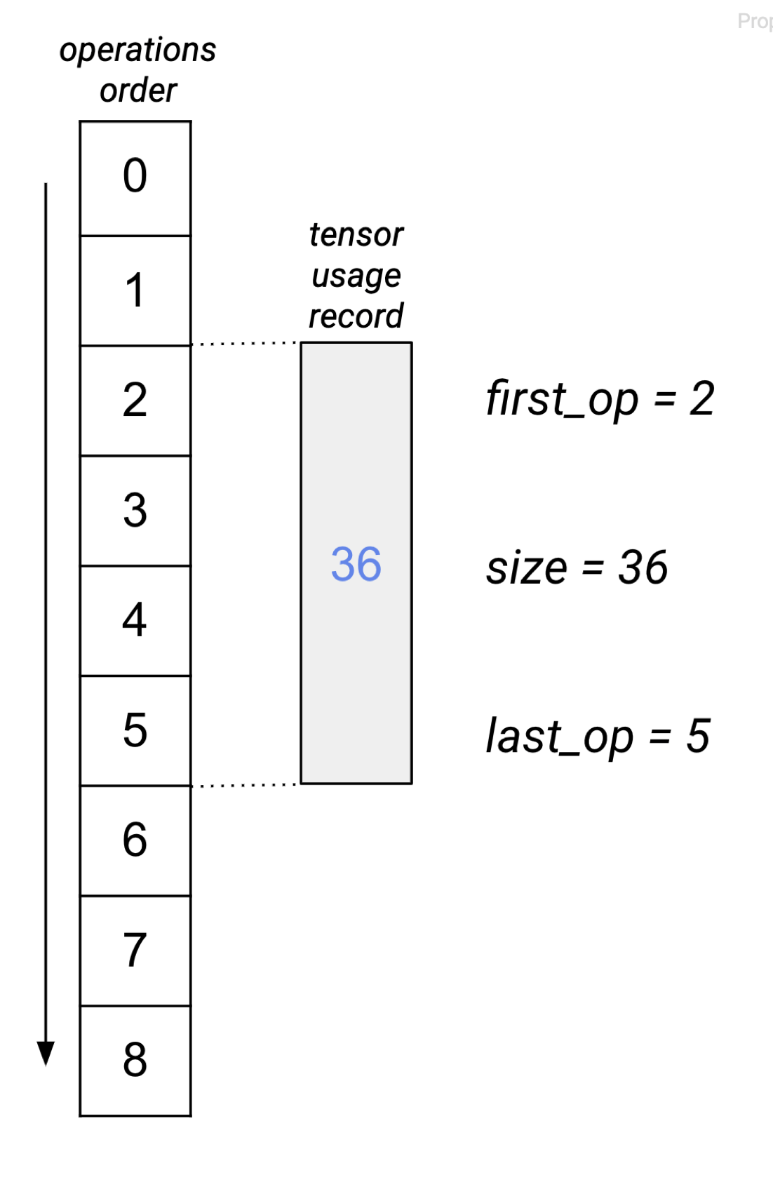
Figure 1: (a) An example neural network with each of its intermediate tensors denoted with its index and its size in black and blue, respectively; note that tensor #8 is not an intermediate tensor. (b) The tensor usage record of tensor #2 as an example.

TensorFlow Lite (TFLite) GPU employs a memory manager for its GPU buffers Lee et al. (2019). Two approximations are explored for this NP-complete resource management problem Sethi (1975), which is similar to register allocation problem, but more complex due to different sizes of tensors. Sekiyama et al. (2018) solve the memory allocation problem as a special case of 2D strip packing problem. We present strategies that outperform these in most cases.

3 Definition of Terms

This section defines several key terms that should facilitate strategy description in the following sections.

Tensor Usage Interval of an intermediate tensor $t$ is defined as the pair $\{\mathit{first\_op_{t}},\mathit{last\_op_{t}}\}$, where $\mathit{first\_op_{t}}$ and $\mathit{last\_op_{t}}$ are the indices of the first and the last operator that use $t$ as its input or output, respectively. The indices are from a topological sort of the neural network which is also the operators’ execution order. For the remainder of the paper, we assume that this order is fixed. Note that no two tensors with intersecting usage intervals can share memory.

Tensor Usage Record of an intermediate tensor $t$ is defined as the triple $\{\mathit{first\_op_{t}},\mathit{last\_op_{t}},\mathit{size_{t}}\}$, where $\mathit{size_{t}}$ is $t$’s aligned size in bytes. Figure 1 illustrates an example neural network and the tensor usage record of tensor #2. The full set of tensor usage records is depicted in Figure 2 (a).

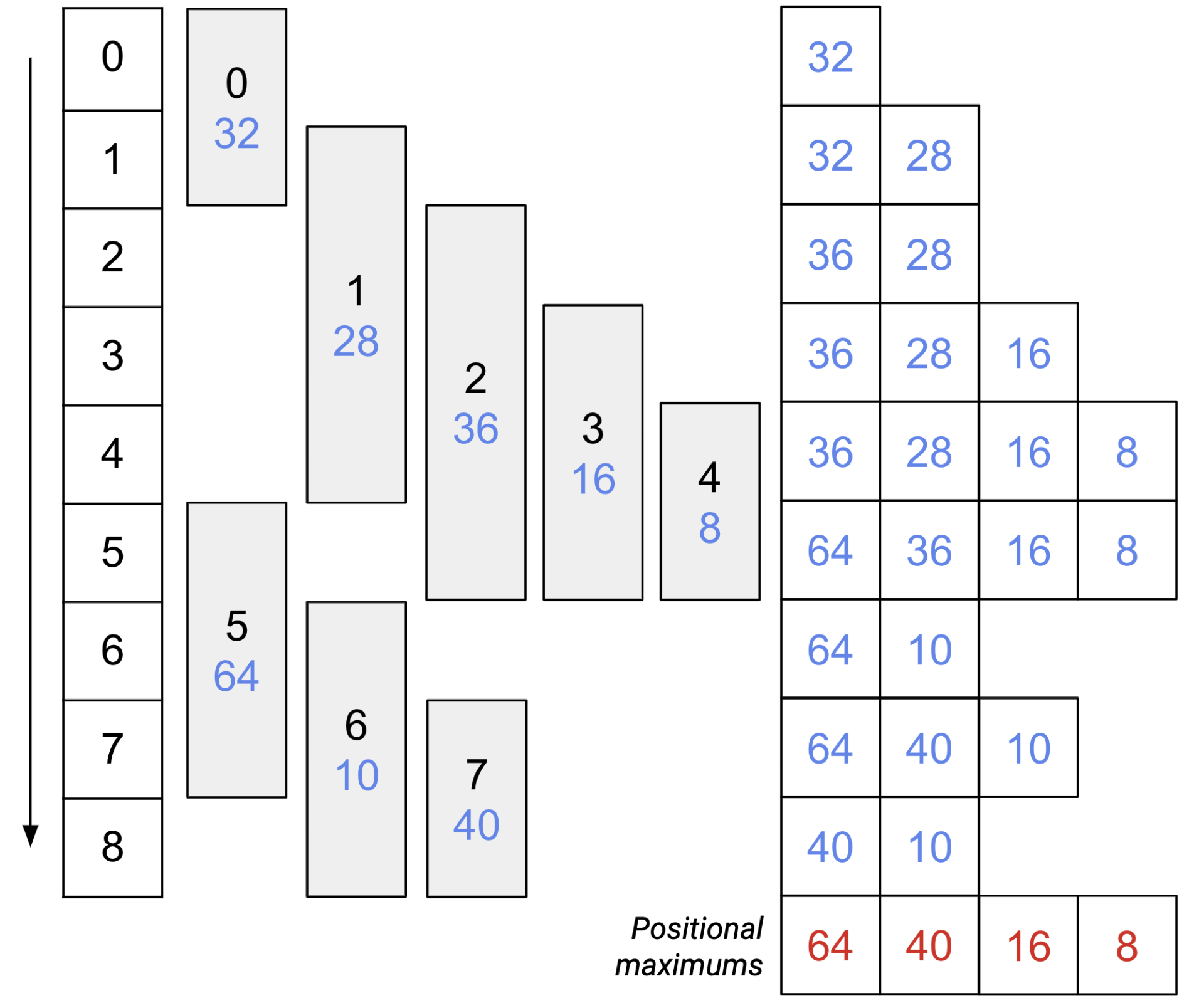
Figure 2: (a) All tensor usage records for the graph in Figure 1 (a). (b) The sorted operator profiles at each execution timestamp; only the tensor sizes are shown in blue. The positional maximums of each column are on the final row, denoted in red.

Operator Profile of an operator $op$ is defined as the set of all tensor usage records $t$ such that $op$ falls between $\mathit{first\_op_{t}}$ and $\mathit{last\_op_{t}}$. Figure 2 (b) visualizes the operator profile of each operator sorted in descending order by size.

Operator Breadth of an operator is defined as the sum of all tensor sizes in its profile. For example, operator #3 in Figure 2 (b) has the operator breadth of $36+28+16=80$.

The $i$-th Positional Maximum is the maximum across $i$-th tensor sizes in descending order for each operator profile. For example, the third positional maximum in Figure 2 (b) is equal to $\mathit{max(16,16,16,10)}=16$.

4 The Shared Objects Approach

There are broadly two ways of sharing memory which are discussed in this and the following section. We call the first Shared Objects where each memory buffer (“shared object”) is assigned to an intermediate tensor at a given time. No two tensors with intersecting usage intervals can be assigned to the same shared object and no shared object can be used for more than one tensor at any moment in time. The size of the shared object is the maximum of all the tensor sizes it is assigned to. The main objective is to minimize the total size of these shared objects. This approach is most suitable for GPU textures.

4.1 Theoretical Lower Bound

Each operator profile is sorted in non-increasing order by its tensor sizes. The largest shared object in the resulting allocation will have a size greater or equal to the largest of first elements across all sorted profiles, and the second largest shared object cannot be less in size than largest of second elements across sorted profiles. This property holds for every shared object. The number of shared objects cannot be less than the largest number of tensors in one operator profile. Thus, the sum of the positional maximums is the theoretical lower bound for the Shared Objects problem. This lower bound may not be achievable for some neural networks.

4.2 Greedy by Breadth

Operator breadths are more correlated for the resulting memory consumption than the order of tensor allocations during inference. Thus, we start from the allocation of tensors that must be present in memory during execution of operator with greater breadth, i.e. Greedy by Breadth (Algorithm 1).

Algorithm 1 Greedy by Breadth for Shared Objects

1:  $\mathit{shared\_objects}\leftarrow\emptyset$

2:  for each $\mathit{t}\in$ tensor usage records do

3:    $\mathit{assigned\_shared\_object_{t}}\leftarrow\mathit{NIL}$

4:  sort $\mathit{operators}$ in non-increasing order of $\mathit{breadth}$

5:  for each $op\in\mathit{operators}$ do

6:    for each $\mathit{t}\in\mathit{profile_{op}}$ do

7:       if $\mathit{assigned\_shared\_object_{t}}\neq\mathit{NIL}$ then

8:         continue

9:       $\mathit{best\_obj}\leftarrow\mathit{NIL}$

10:       for each $obj\in\mathit{shared\_objects}$ do

11:         $\mathit{is\_better}\leftarrow\mathit{TRUE}$

12:         if $\mathit{best\_obj}\neq\mathit{NIL}$ then

13:          if $\mathit{best\_obj.size}<\mathit{size_{t}}$

14:            if $\mathit{obj.size}\leq\mathit{best\_obj.size}$ then

15:              $\mathit{is\_better}\leftarrow\mathit{FALSE}$

16:          elseif $\mathit{obj.size}\geq\mathit{best\_obj.size}$ or           $\mathit{obj.size}<\mathit{size_{t}}$ then

17:            $\mathit{is\_better}\leftarrow\mathit{FALSE}$

18:         $\mathit{suitable}\leftarrow\mathit{TRUE}$

19:         for each $\mathit{x}\in$ tensor usage records do

20:          $\mathit{max\_first\_op}\leftarrow\max(\mathit{first\_op_{t}},\mathit{first\_op_{x}})$

21:          $\mathit{min\_last\_op}\leftarrow\min(\mathit{last\_op_{t}},\mathit{last\_op_{x}})$

22:          if $\mathit{assigned\_shared\_object_{x}}=\mathit{obj}$ and          $max\_first\_op\leq min\_last\_op$ then

23:            $\mathit{suitable}\leftarrow\mathit{FALSE}$

24:         if $\mathit{suitable}$ and $\mathit{is\_better}$ then

25:          $\mathit{best\_obj}\leftarrow\mathit{obj}$

26:       if $\mathit{best\_obj}=\mathit{NIL}$ then

27:         $\mathit{best\_obj}\leftarrow$ new shared object with size $\mathit{size_{t}}$

28:         $\mathit{shared\_objects}$.insert($\mathit{best\_obj}$)

29:       else

30:         $\mathit{best\_obj.size}\leftarrow\max(\mathit{best\_obj.size},\mathit{size_{t}})$

31:       $\mathit{assigned\_shared\_object_{t}}\leftarrow\mathit{best\_obj}$

Operators are sorted in non-increasing order by their breadth (L.4). For each operator in this sorted ordering, we assign shared objects to tensors from its profile, but only for those that have not been assigned yet (L.7). If there are several such tensors, we start from the largest by size. A shared object $s$ is suitable for assignment to tensor $t$, if and only if there is no tensor $u$, such that $s$ is assigned to the $u$ and usage intervals of $t$ and $u$ overlap (L.18–23). Shared object assignment (L.12–17, 24–28) can be summarized as:

• If there are suitable shared objects not smaller than $size_{t}$, assign the smallest to $t$.

• If all suitable shared objects are smaller than $size_{t}$, update the largest size to $size_{t}$ and assign it to $t$.

• If there are no suitable shared objects, create a new shared object with size $size_{t}$ and assign it to $t$.

Figure 3: Greedy by Breadth for Shared Objects on the neural network in Figure 1.

The algorithm has a run-time complexity of $O(kn^{2})$, where $k$ and $n$ are the number of shared objects and intermediate tensors, respectively, when implemented naïvely. Note that $k$ is often at lower tens, whereby $n$ is one or two magnitudes larger in a typical neural network. With an interval tree for each shared object that stores the usage intervals of all tensors, the complexity can be reduced to $O(kn\log n)$. An example output is shown in Figure 3.

4.3 Greedy by Size

Algorithm 2 Greedy by Size for Shared Objects

1:  sort tensor usage records in non-increasing order of $\mathit{size}$

2:  $\mathit{shared\_objects}\leftarrow\emptyset$

3:  for each $\mathit{t}\in$ tensor usage records do

4:    $\mathit{assigned\_shared\_object_{t}}\leftarrow\mathit{NIL}$

5:  for each $\mathit{t}\in$ tensor usage records do

6:     $\mathit{best\_obj}\leftarrow\mathit{NIL}$

7:     for each $obj\in\mathit{shared\_objects}$ do

8:       $\mathit{suitable}\leftarrow\mathit{TRUE}$

9:       for each $\mathit{x}\in$ tensor usage records do

10:         $\mathit{max\_first\_op}\leftarrow\max(\mathit{first\_op_{t}},\mathit{first\_op_{x}})$

11:         $\mathit{min\_last\_op}\leftarrow\min(\mathit{last\_op_{t}},\mathit{last\_op_{x}})$

12:         if $\mathit{assigned\_shared\_object_{x}}=\mathit{obj}$ and         $\mathit{max\_first\_op}\leq\mathit{min\_last\_op}$ then

13:          $\mathit{suitable}\leftarrow\mathit{FALSE}$

14:       if $\mathit{suitable}$ then

15:         $\mathit{best\_obj}\leftarrow\mathit{obj}$

16:     if $\mathit{best\_obj}=\mathit{NIL}$ then

17:       $\mathit{best\_obj}\leftarrow$ new shared object with size $\mathit{size_{t}}$

18:       $\mathit{shared\_objects}$.insert($\mathit{best\_obj}$)

19:     $\mathit{assigned\_shared\_object_{t}}\leftarrow\mathit{best\_obj}$

While the operator breadth is significant, it is a number derived from tensor sizes in the operator profiles. Thus, we explore another strategy Greedy by Size where the tensor sizes are the most significant feature (Algorithm 2).

We iterate through intermediate tensors in non-increasing order of their size (L.1,5), and for each tensor $t$ find suitable shared object to assign to it (L.8–11), similar to Greedy by Breadth. As before, there are no shared objects in the beginning (L.2). The assignment becomes even easier, because we prefer larger tensors over smaller ones, i.e. the shared object size never increases, and only two steps remain:

• Assign the smallest suitable shared object to $t$ if it exists.

• If there are no suitable shared objects, create a new shared object with size $size_{t}$ and assign it to $t$.

Greedy by Size has the same complexity as Greedy by Breadth. Its example output is shown in Figure 4.

4.4 Greedy by Size Improved

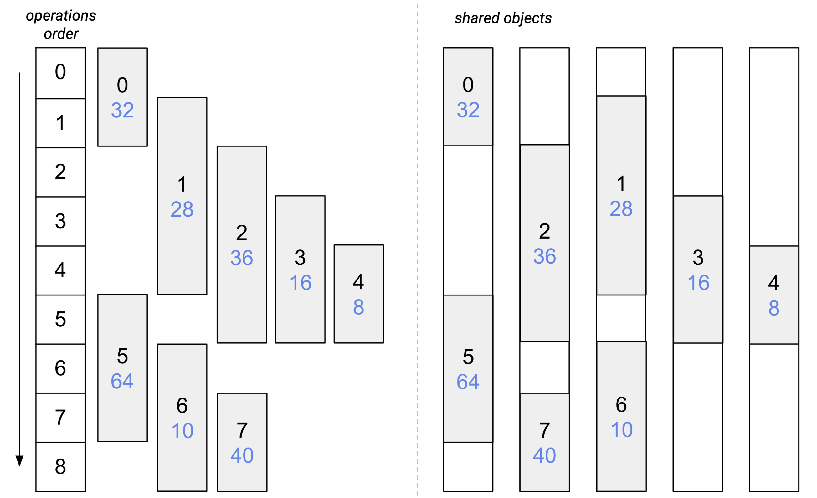
Figure 4: Greedy by Size for Shared Objects on the neural network in Figure 1.

While refining Greedy by Size, we observed that there were close mis-assignments that prevented it from reaching the lower bound. If there was a wiggle room for tensors with similar sizes, it could have reached the optimum.

As the theoretical lower bound of Shared Objects is determined by positional maximums, we split Greedy by Size into stages by positional maximum. In the first stage, we assign all tensors with size equal to largest positional maximum. In the second stage, we assign all tensors with sizes less than the largest positional maximum, but greater than the second positional maximum. In the third stage, we assign all tensors with sizes equal to the second positional maximum, etc. until all the tensors are assigned. We consider all tensors in one stage to have almost equal significance. This is based on the results of the experiments with greedy algorithms on different neural networks: final result is usually pretty close to the theoretical lower bound, and most of the shared objects, especially larger ones, often have the same sizes as in the lower bound.

Another improvement we propose is the order of tensors assignment inside of one stage. Tensor sizes in one stage are almost equal, so we choose such a pair of tensor and shared object that result in the smallest possible time gap when shared object is not in use, i.e. find such pair of tensor $t$ form current stage and suitable shared object $s$ for it, that distance between usage interval for $t$ and closest usage interval from tensors, previously assigned to $s$, is the smallest possible. It means, that we find shared object that still can be used for tensor $t$ assignment, but the gap when this shared object is not used right before or right after tensor $t$ usage interval is the smallest possible.

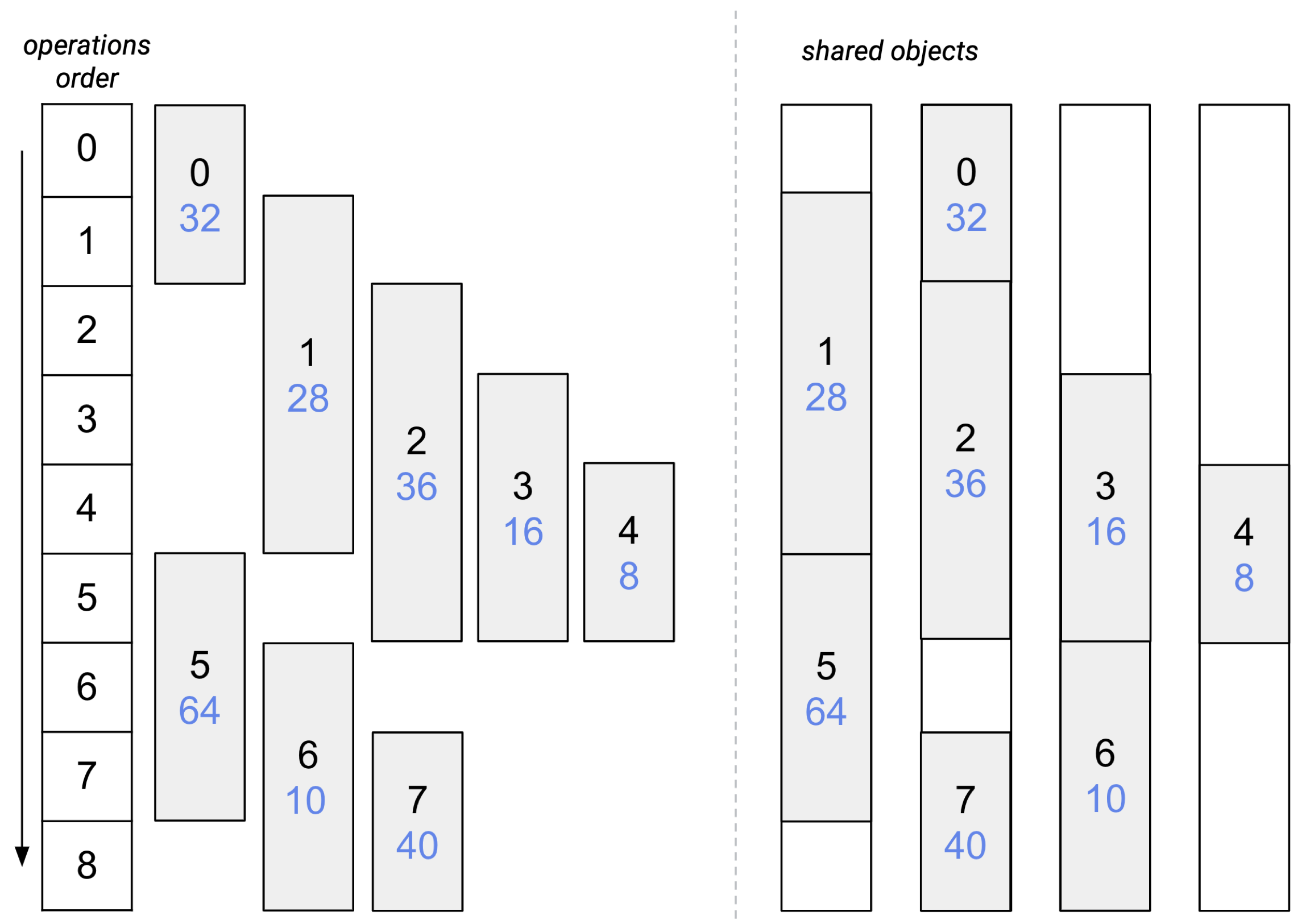
Figure 5: Greedy by Size Improved for Shared Objects on the neural network in Figure 1.

These improvements can be implemented without changing the complexity of Greedy by Size. The algorithm assigns shared objects to tensors, using the order defined by positional maximums from  2. Figure 5 visualizes this strategy. The results of experiments confirm that using Greedy by Size Improved provides us with better or the same result, compared to the original without improvements.

5 The Offset Calculation Approach

We call the other memory sharing approach Offset Calculation where a large chunk of memory is pre-allocated and the intermediate tensors are given parts of the memory by the offsets within the memory block. The main objective is to minimize the size of the allocated memory block. While the solution to this problem shows best performance in terms of total allocated memory, it is only applicable to CPU memory or GPU buffers, but not GPU textures which need to be accessed as a whole. The solution of Shared Objects problem can be converted to the solution of Offset Calculation problem by placing the shared objects contiguously in memory. The opposite is not true as memory footprints of tensors with non-intersecting usage intervals can still overlap.

The Offsets Calculation problem can be seen as a special case of 2D strip packing problem Sekiyama et al. (2018). A set of rectangular items with fixed coordinates by one axes into a container to minimize its size by other dimension. If the height of a container is treated as the allocation time axis, then we need to minimize the container’s width which corresponds to the memory footprint.

5.1 Theoretical Lower Bound

During the execution of any operator of the neural network all tensors in its profile need to be present in memory. Their total size is equal to this operator’s breadth. It means, that any strategy will provide us with memory consumption greater or equal to any operator breadth, and the lower bound for Offset Calculation is equal to the maximum among all operator breadths. The lower bound cannot be always achieved, but our methods achieve the lower bound in most cases.

5.2 Greedy by Size for Offset Calculation

As Greedy by Size works well for Shared Objects, we employ a similar method for Offsets Calculation (Algorithm 3).

Algorithm 3 Greedy by Size for Offset Calculation

1:  sort tensor usage records in non-increasing order of $\mathit{size}$

2:  for each $\mathit{t}\in$ tensor usage records do

3:    $\mathit{assigned\_offset_{t}}\leftarrow\mathit{NIL}$

4:  $\mathit{total\_consumption}\leftarrow\mathit{0}$

5:  $\mathit{ordered\_allocated\_ids}\leftarrow\emptyset$

6:  for each $\mathit{t}\in$ tensor usage records do

7:     $\mathit{prev\_offset}\leftarrow\mathit{0}$

8:     $\mathit{best\_offset}\leftarrow\mathit{NIL}$

9:     $\mathit{smallest\_gap}\leftarrow\infty$

10:     for each $\mathit{x}\in\mathit{ordered\_allocated\_ids}$ do

11:       $\mathit{max\_first\_op}\leftarrow\max(\mathit{first\_op_{t}},\mathit{first\_op_{x}})$

12:       $\mathit{min\_last\_op}\leftarrow\min(\mathit{last\_op_{t}},\mathit{last\_op_{x}})$

13:       if $\mathit{max\_first\_op}\leq\mathit{min\_last\_op}$ then

14:         $\mathit{gap}\leftarrow\mathit{offset_{x}}-\mathit{prev\_offset}$

15:         if $\mathit{gap}\geq\mathit{size_{t}}$ then $\mathit{gap}<\mathit{smallest\_gap}$ then

16:          $\mathit{smallest\_gap}\leftarrow\mathit{gap}$

17:          $\mathit{best\_offset}\leftarrow\mathit{prev\_offset}$

18:       $\mathit{prev\_offset}\leftarrow\max(\mathit{prev\_offset},\mathit{offset_{x}}+\mathit{size_{x}})$

19:     if $\mathit{best\_offset}=\mathit{NIL}$ then

20:       $\mathit{best\_offset}\leftarrow$ $\mathit{prev\_offset}$

21:     $\mathit{offsets_{t}}\leftarrow$ $\mathit{best\_offset}$

22:     $\mathit{total\_consumption}\leftarrow$      $\max(\mathit{total\_consumption},\mathit{best\_offset}+\mathit{size_{t}})$

23:     insert $\mathit{t}$ into $\mathit{ordered\_allocated\_ids}$

We first iterate through tensor usage records in non-increasing order by their $size$ (L.1,6). For each record, we check already assigned tensors whose usage intervals intersect with that of the current tensor (L.10–13) to find the smallest gap in memory between them such that current tensor fits into that gap (L.9,14–17). If such a gap is found, the current tensor is allocated to this gap. Otherwise, we allocate it after the rightmost tensor whose usage interval intersect with that of the current tensor (L.19–20). We assign the corresponding offset to current tensor and the tensor becomes assigned (L.21–23) as shown in Figure 6.

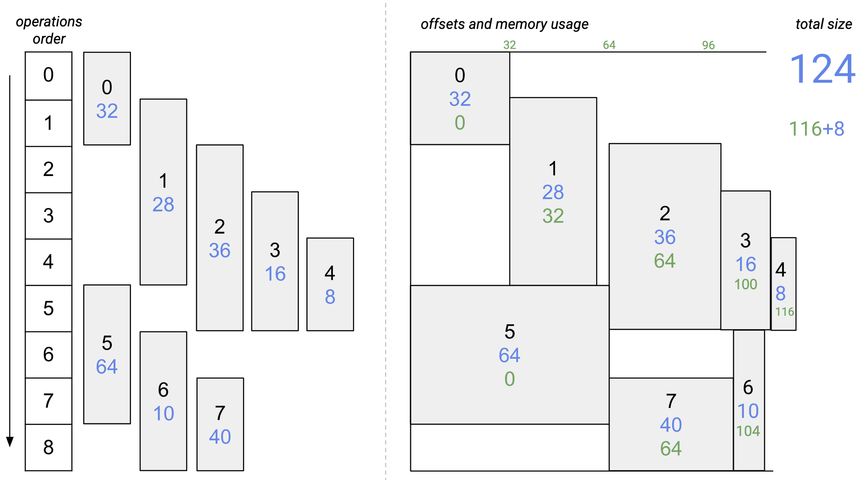
Figure 6: Greedy by Size for Offset Calculation on the neural network in Figure 1.

5.3 Greedy by Breadth for Offset Calculation

Greedy by Breadth can also be converted for Offsets Calculation in a similar fashion. Specifically:

• Iterate through all operators in non-increasing order by their breadth.

• For each operator in this order, iterate through all tensors from its profile that have not been assigned yet, in non-increasing order of their size.

• To calculate the offset for the tensor, use the same logic of finding the smallest gap as in Alg. 3 (L.7–23). At the end of this step, the tensor is marked as assigned.

While Greedy by Breadth does not perform well for Offset Calculation compared to Greedy by Size, it still outperforms the prior work on some networks, e.g. MobileNet v2.

Table 1: Memory footprint of Shared Objects strategies (in MB; best results in bold). The first 3 rows are our strategies, the next 2 are prior work, and the last 2 serve as baseline.

Strategy	MobileNet v1	MobileNet v2	DeepLab v3	Inception v3	PoseNet	BlazeFace
Greedy by Size	4.594	7.178	6.437	10.337	6.347	0.592
Greedy by Size Improved	4.594	6.891	6.437	10.337	6.347	0.518
Greedy by Breadth	6.125	6.699	6.437	10.676	8.390	0.675
Greedy Lee et al. (2019)	4.594	8.039	7.168	12.703	6.347	0.587
Min-cost Flow Lee et al. (2019)	5.359	7.513	8.364	10.624	7.359	0.582
Lower Bound	4.594	6.604	6.105	8.955	6.347	0.518
Naïve	19.248	26.313	48.642	54.010	28.556	2.698

Table 2: Memory footprint of Offset Calculation strategies (in MB; best results in bold). The first 2 rows are our strategies, the next 2 are prior work, and the last 2 serve as baseline.

Strategy	MobileNet v1	MobileNet v2	DeepLab v3	Inception v3	PoseNet	BlazeFace
Greedy by Size	4.594	5.742	4.653	7.914	6.271	0.492
Greedy by Breadth	4.594	5.742	4.653	7.914	7.359	0.656
Greedy Lee et al. (2019)	6.125	6.508	4.985	10.624	8.362	0.492
Strip Packing Sekiyama et al. (2018)	4.594	6.029	4.321	7.914	6.271	0.533
Lower Bound	4.594	5.742	4.320	7.914	6.271	0.492
Naïve	19.248	26.313	48.642	54.010	28.556	2.698

6 Evaluation

We compare our strategies with Greedy Lee et al. (2019), Min-cost Flow Lee et al. (2019), and Strip Packing Bestfit Sekiyama et al. (2018) on MobileNet v1 Howard et al. (2017), MobileNet v2 Sandler et al. (2018), DeepLab v3 Chen et al. (2017), Inception v3 Szegedy et al. (2016), PoseNet Kendall et al. (2015), and BlazeFace Bazarevsky et al. (2019), at 32-bit precision floating point, but the strategies can be generalized to any data type.

The best results for Shared Objects are achieved with Greedy by Size Improved on all networks except MobileNet v2, for which Greedy by Breadth does better (Table 1). Compared to prior work, our strategies do up to 11% better, and compared to naïve strategy, they do up to 7.5$\times$ better. The most significant improvement is seen for DeepLab with all three described strategies, for MobileNet v2 with Greedy by Breadth, and for BlazeFace with Greedy by Size Improved. Our strategies reach the theoretical lower bound for MobileNet v1, PoseNet, and BlazeFace, and are within 16% of the lower bound for the other networks. For inference engines needing the Shared Objects approach, it is recommended to default to Greedy by Size Improved.

For Offset Calculation, Greedy by Size performs best as shown in Table 2. It achieves the theoretical lower bound on all selected neural networks, except DeepLab, where it still falls within 8% of the lower bound. Moreover, it provides us with memory allocation consuming up to 25% less memory for intermediate tensors than Greedy, up to 7.7% less than in Strip Packing Bestfit, and up to 10.5 times less than in a naïve strategy. Only for DeepLab, Strip Packing Bestfit shows 7.2% better allocation that is very close to the theoretical lower bound. For inference engines requiring the Offset Calculation approach, it is recommended to evaluate both Greedy by Size and Strip Packing Bestfit before the first inference and select the superior performing strategy.

7 Conclusion

We presented five novel strategies for efficiently sharing memory buffers among intermediate tensors in deep neural networks to minimize the memory footprint of the inference engine at the edge. The experiments showed that our strategies get the inference run-time’s memory footprint to equal to or close to the theoretical lower bound.

The presented strategies for either approach are fast enough (a few milliseconds for most networks), so that they can be explored at run-time for the smallest memory footprint. In general, i.e. CPU inference or GPU inference with buffers, it is recommended to explore the two best strategies for the Offset Calculation problem, Greedy by Size and Strip Packing Bestfit. For the Shared Objects problem, e.g. GPU inference with textures, Greedy by Size Improved and Greedy by Breadth are recommended for pre-inference exploration.

The strategies presented assume that the sizes of intermediate tensors are known in advance. This assumption may not be true for recurrent neural networks with long short-term memory units Hochreiter & Schmidhuber (1997) including intermediate tensors with dynamically changing sizes. For such cases, the algorithms need to be run multiple times saving information about allocation from all runs in one place. The first run will allocate only those tensors whose sizes are known at the beginning, and the second run will allocate those tensors whose sizes become known after calculation of the first dynamic tensor, etc.

7.1 Future Work

The operator indices in tensor usage records and intervals are defined by the topological sort of the neural network. Optimizing the sorting algorithm for the smallest possible memory footprint is a potential future research topic.

The current choice for the best strategy only focuses on the memory footprint. Other criteria such as cache hit rate and inference latency can be incorporated into evaluation for fast inference on resource-constrained systems.

References

- Bazarevsky et al. (2019) Bazarevsky, V., Kartynnik, Y., Vakunov, A., Raveendran, K., and Grundmann, M. Blazeface: Sub-millisecond neural face detection on mobile gpus. arXiv preprint arXiv:1907.05047, 2019.
- Bergstra et al. (2010) Bergstra, J., Breuleux, O., Bastien, F., Lamblin, P., Pascanu, R., Desjardins, G., Turian, J., Warde-Farley, D., and Bengio, Y. Theano: A cpu and gpu math expression compiler. In Proceedings of the 9th Python in Science Conference, pp. 3–10, 2010.
- Chen et al. (2017) Chen, L.-C., Papandreou, G., Kokkinos, I., Murphy, K., and Yuille, A. L. Deeplab: Semantic image segmentation with deep convolutional nets, atrous convolution, and fully connected crfs. IEEE transactions on pattern analysis and machine intelligence, 40(4):834–848, 2017.
- Chen et al. (2015) Chen, T., Li, M., Li, Y., Lin, M., Wang, N., Wang, M., Xiao, T., Xu, B., Zhang, C., and Zhang, Z. Mxnet: A flexible and efficient machine learning library for heterogeneous distributed systems. In NIPS Workshop on Machine Learning Systems (LearningSys), 2015.
- Chen et al. (2016) Chen, T., Xu, B., Zhang, C., and Guestrin, C. Training deep nets with sublinear memory cost. arXiv preprint arXiv:1604.06174, 2016.
- He et al. (2016) He, K., Zhang, X., Ren, S., and Sun, J. Deep residual learning for image recognition. In Proceedings of the IEEE Conference on Computer Vision and Pattern Recognition, pp. 770–778, 2016.
- Hochreiter & Schmidhuber (1997) Hochreiter, S. and Schmidhuber, J. Long short-term memory. Neural computation, 9(8):1735–1780, 1997.
- Howard et al. (2017) Howard, A. G., Zhu, M., Chen, B., Kalenichenko, D., Wang, W., Weyand, T., Andreetto, M., and Adam, H. Mobilenets: Efficient convolutional neural networks for mobile vision applications. arXiv preprint arXiv:1704.04861, 2017.
- Kendall et al. (2015) Kendall, A., Grimes, M., and Cipolla, R. Posenet: A convolutional network for real-time 6-dof camera relocalization. In Proceedings of the IEEE international Conference on Computer Vision, pp. 2938–2946, 2015.
- Lee et al. (2019) Lee, J., Chirkov, N., Ignasheva, E., Pisarchyk, Y., Shieh, M., Riccardi, F., Sarokin, R., Kulik, A., and Grundmann, M. On-device neural net inference with mobile gpus. In CVPR Workshop for Efficient Deep Learning for Computer Vision (ECV2019), 2019.
- Li et al. (2016) Li, C., Yang, Y., Feng, M., Chakradhar, S., and Zhou, H. Optimizing memory efficiency for deep convolutional neural networks on gpus. In SC’16: Proceedings of the International Conference for High Performance Computing, Networking, Storage and Analysis, pp. 633–644. IEEE, 2016.
- Sandler et al. (2018) Sandler, M., Howard, A., Zhu, M., Zhmoginov, A., and Chen, L.-C. Mobilenetv2: Inverted residuals and linear bottlenecks. In Proceedings of the IEEE Conference on Computer Vision and Pattern Recognition, pp. 4510–4520, 2018.
- Sekiyama et al. (2018) Sekiyama, T., Imamichi, T., Imai, H., and Raymond, R. Profile-guided memory optimization for deep neural networks. arXiv preprint arXiv:1804.10001, 2018.
- Sethi (1975) Sethi, R. Complete Register Allocation Problems. SIAM Journal on Computing, 4:226–248, 1975.
- Szegedy et al. (2016) Szegedy, C., Vanhoucke, V., Ioffe, S., Shlens, J., and Wojna, Z. Rethinking the inception architecture for computer vision. In Proceedings of the IEEE Conference on Computer Vision and Pattern Recognition, pp. 2818–2826, 2016.
- Wu et al. (2019) Wu, C.-J., Brooks, D., Chen, K., Chen, D., Choudhury, S., Dukhan, M., Hazelwood, K., Isaac, E., Jia, Y., Jia, B., et al. Machine learning at facebook: Understanding inference at the edge. In 2019 IEEE International Symposium on High Performance Computer Architecture (HPCA), pp. 331–344. IEEE, 2019.