Multifractality meets entanglement: relation for non-ergodic extended states

Abstract

In this work we establish a relation between entanglement entropy and fractal dimension $D$ of generic many-body wave functions, by generalizing the result of Don N. Page [Phys. Rev. Lett. 71, 1291] to the case of sparse random pure states (S-RPS). These S-RPS living in a Hilbert space of size $N$ are defined as normalized vectors with only $N^{D}$ ($0\leq D\leq 1$) random non-zero elements. For $D=1$ these states used by Page represent ergodic states at infinite temperature. However, for $0<D<1$ the S-RPS are non-ergodic and fractal as they are confined in a vanishing ratio $N^{D}/N$ of the full Hilbert space. Both analytically and numerically, we show that the mean entanglement entropy ${\mathcal{S}_{1}}(A)$ of a subsystem $A$, with Hilbert space dimension $N_{A}$, scales as $\overline{\mathcal{S}_{1}}(A)\sim D\ln N$ for small fractal dimensions $D$, $N^{D}<N_{A}$. Remarkably, $\overline{\mathcal{S}_{1}}(A)$ saturates at its thermal (Page) value at infinite temperature, $\overline{\mathcal{S}_{1}}(A)\sim\ln N_{A}$ at larger $D$. Consequently, we provide an example when the entanglement entropy takes an ergodic value even though the wave function is highly non-ergodic. Finally, we generalize our results to Renyi entropies $\mathcal{S}_{q}(A)$ with $q>1$ and to genuine multifractal states and also show that their fluctuations have ergodic behavior in narrower vicinity of the ergodic state, $D=1$.

Introduction– The success of classical statistical physics is based on the concept of ergodicity, which allows the description of complex systems by the knowledge of only few thermodynamic parameters Landau and Lifshitz (2013); Boltzmann (1995). In quantum realm the paradigm of ergodicity is much less understood and its characterization is now an active research front.

The most accredited theory, which gives an attempt to explain equilibration in closed quantum systems, relies on the eigenstate thermalization hypothesis (ETH) Deutsch (1991); Srednicki (1994, 1996); Rigol et al. (2008). ETH assets that the system thermalizes locally at the level of single eigenstates and has been tested numerically in a wide variety of generic interacting systems D’Alessio et al. (2016); Rigol et al. (2008).

It is now well established that entanglement plays a fundamental role on the thermalization process Nandkishore and Huse (2015); Abanin et al. (2019); Alet and Laflorencie (2018); D’Alessio et al. (2016); Amico et al. (2008). Thermal states are locally highly entangled with the rest of the system, which acts as a bath. Consequently, the measurement of entanglement entropy (EE) has been found to be a resounding resource to probe ergodic/thermal phases, both theoretically Luitz et al. (2015); Kjäll et al. (2014); Geraedts et al. (2016); Serbyn et al. (2016); De Tomasi et al. (2017); Khemani et al. (2017) and recently also experimentally Islam et al. (2015); Kaufman et al. (2016); Chiaro et al. (2019); Lukin et al. (2019). For instance, infinite temperature ergodic states are believed to behave like random vectors Deutsch (1991); D’Alessio et al. (2016) and their EE reaches a precise value often referred as Page value Page (1993).

On the other hand, ergodicity is deeply connected to the notion of chaos Haake (2006); D’Alessio et al. (2016), which implies also an equipartition of the many-body wave function over the available many-body Fock states, usually quantified by multifractal analysis, e.g., by scaling of the inverse participation ratio (IPR) Evers and Mirlin (2008). In this case, infinite temperature ergodic states span homogeneously the entire Hilbert space WE- . The latter states should be distinguished from the so-called non-ergodic extended (NEE) states. These NEE states live on a fractal in the Fock space, which is a vanishing portion of the total Hilbert space. Recently, the NEE have been invoked to understand new phases of matter like bad metals De Luca et al. (2014a); Kravtsov et al. (2015); Altshuler et al. (2016); Pino et al. (2017); Kravtsov et al. (2018); Bera et al. (2018); De Tomasi et al. (2020); Tomasi et al. (2019); Kravtsov et al. (2020), which are neither insulators nor conventional diffusive metals and also are found in chaotic many-body quantum system like in the Sachdev-Ye-Kitaev model Micklitz et al. (2019); H. Wang (2019); Kamenev (2018).

Very recently, the two aforementioned probes, EE and IPR, have been used to describe thermal phases (specially at infinite temperature), and to detect ergodic-breaking quantum phase transitions Serbyn et al. (2013); Luitz et al. (2015, 2019); Macé et al. (2019); Monthus (2016). Nevertheless, the relations between these two probes has not been studied extensively so far EE_ . Thus, the natural question arises: to what extend do these probes lead to the same description?

In this work, we build up a bridge between ergodic properties extracted from EE and the ones from multifractal analysis. With this aim, we generalize the seminal work of Page Page (1993), computing EE and its fluctuations for NEE states. Remarkably, we show, both analytically and numerically, that a subsystem EE can still be ergodic (Page value), even though the states are highly non-ergodic. Consequently, the mean value of EE might be not enough to state ergodicity, though EE reaches the Page value.

General definitions– The Renyi entropy, $\mathcal{S}_{q}(A)$, of a subsystem $A$ with Hilbert space dimensions $N_{A}=N^{p}$, $p\leq 1/2$, is defined as:

$$\mathcal{S}_{q}(A)=\frac{\ln\Sigma_{q}}{1-q}\ ,\text{ with }\Sigma_{q}={\rm Tr}_{A}[\rho_{A}^{q}]=\sum_{M=1}^{N_{A}}\lambda_{M}^{q},\$$ (1)

where $\rho_{A}={\rm Tr}_{B}[\rho]$ is the reduced density matrix of the subsystem $A$, after tracing out the subsystem $B=A^{c}$ and $\{\lambda_{M}\}$ are Schmidt eigenvalues of $\rho_{A}$. The von Neumann EE, $\mathcal{S}_{1}(A)=\lim_{q\rightarrow 1}\mathcal{S}_{1}(A)$ equals to $-{\rm Tr}_{A}[\rho_{A}\ln{\rho_{A}}]$. For a pure state $\rho=\left|\psi\right\rangle\left\langle\psi\right|$,

$$\rho^{A}_{M,M^{\prime}}=\sum_{m=1}^{N_{B}}\psi_{M,m}\psi_{M^{\prime},m}^{*}\ ,$$ (2)

where $\psi_{M,m}$ are the wave function coefficients $\left|\psi\right\rangle=\sum_{M=0}^{N_{A}-1}\sum_{m=0}^{N_{B}-1}\psi_{M,m}\left|M\right\rangle_{A}\otimes\left|m\right\rangle_{B}$ in the computational basis $\left|M\right\rangle_{A}$, $1\leq M\leq{N_{A}}$, and $\left|m\right\rangle_{B}$, $1\leq m\leq{N_{B}}$, of the two subsystems $A$ and $B$, respectively.

For fully random states, $D=1$, the mean von Neumann EE is given by the Page value Page (1993)

$$\overline{\mathcal{S}_{{\rm Page}}}(A)=\ln N_{A}-\frac{N_{A}}{2N_{B}},$$ (3)

and its fluctuations decays to zero, $\overline{\delta\mathcal{S}_{{\rm Page}}}(A)=(\overline{\mathcal{S}^{2}}(A)-\overline{\mathcal{S}}^{2}(A))^{1/2}\sim N_{B}^{-1}$ Nadal et al. (2010, 2011); Vivo et al. (2016). The overline indicates the random vector average.

Moreover, the ergodic properties of the wave function $\{\psi_{\mathbb{n}=(M,m)}\}$ can be characterized in terms of multifractal analysis Evers and Mirlin (2008) via the fractal dimensions $D_{q}$, ${q\geq 0}$, defined through the scaling of the inverse participation ratios ${\rm IPR}_{q}$ with $N$,

$$D_{q}\ln{N}=\frac{\ln{\rm IPR}_{q}}{1-q}\ ,\text{ with }{\rm IPR}_{q}=\sum_{\mathbb{n}}|\psi_{\mathbb{n}}|^{2q},$$ (4)

giving in the limit $q\rightarrow 1$, $D_{1}\ln{N}=-\sum_{\mathbb{n}}|\psi_{\mathbb{n}}|^{2}\ln|\psi_{\mathbb{n}}|^{2}$.

The exponent $D_{1}$ provides important information on the dimension of the support set of the wave function in the Fock space, which scales as $\sim N^{D_{1}}$ De Luca et al. (2014b). Ergodic states are characterized by $D_{q}=1$, meaning that the state is homogeneously spread over the entire Hilbert space WE- . Instead, NEE states are usually multifractal with $D_{q}<1$ and their support set is a vanishing ratio of the full Hilbert space $\sim N^{D_{1}}/N$.

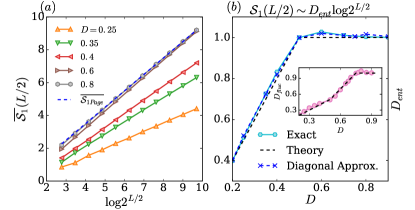
Figure 1: von Neumann EE scaling versus fractal dimension $D$ for S-RPS. (a) $\overline{\mathcal{S}_{1}}(L/2)$ of half-system, $N_{A}=2^{L/2}$, versus $L$ for different $D$; dashed line shows the Page value, Eq. (3). (b) Slope $D_{ent}$ of $\overline{\mathcal{S}_{1}}(L/2)\sim D_{ent}L/2\ln{2}$ versus $D$ (Exact) and of $-\sum_{i}\rho_{M,M}\ln{\rho_{M,M}}\sim D_{ent}L/2\ln{2}$ (Diagonal Approx.); black line represents the theoretical prediction in Eq. (7). (inset) Slope $D_{fluc}$ of the standard deviation $\overline{\delta\mathcal{S}}(L/2)\sim D_{fluc}\ln{2^{L/2}}$ versus $D$. Black dashed line shows analytical prediction, Eq. (64), for $p=1/2$.

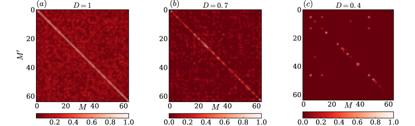
Figure 2: Structure of half-system reduced density matrix $|\rho_{A}^{M,M^{\prime}}|/\max_{M,M^{\prime}}|\rho_{A}^{M,M^{\prime}}|$ for S-RPS with (a) $D=1$, (b) $D=0.7$, and (c) $D=0.4$ for $N_{A}=2^{L/2}$ and $L=12$. In all panels $\rho_{A}$ is mostly represented by the diagonal elements with almost uniform distribution $\rho_{A}^{M,M}\sim N_{A}^{-1}$ for $D>1/2$ (a, b) and bimodal distribution otherwise (c). The latter case is given by $\sim 2^{DL}$ non-zero nearly uniform elements normalized as $\rho_{A}^{M,M}\sim 2^{-DL}$ with the rest being negligibly small. The corresponding EE saturates at the ergodic Page value $\overline{\mathcal{S}_{1}}(A)=\overline{\mathcal{S}_{\rm Page}}(A)$ for $D>1/2$, while being dominated by $2^{DL}$ non-zero elements for $D<1/2$ leading to $\overline{\mathcal{S}_{1}}(A)\simeq-\sum_{M}\rho_{A}^{M,M}\ln{\rho_{A}^{M,M}}\sim DL\ln{2}$.

In this work, we consider entanglement properties of NEE states by introducing the sparse random pure states (S-RPS). The S-RPS are normalized random vectors $\{\psi_{\mathbb{n}}\}$ with $N^{D}$ non-zero elements, that are randomly distributed over the Hilbert space. Similarly to RPS Page (1993) ($D=1$) all non-zero coefficients are Gaussian distributed with the normalization-controlled width. The S-RPS are described by only one fractal dimension $D_{q}=D<1$, ${\rm IPR}_{q}\sim N^{D(1-q)}$, $q>0$ MF- . Thus, the S-RPS are homogeneously spread, but only in a vanishing ratio of the total Hilbert space.

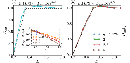
Figure 3: Effect of partition size and scaling of Renyi EE. (a) Slope $D_{ent}$ of the mean EE versus fractal dimension $D$ with $N_{A}=2^{L/3}$. (inset) $\overline{\mathcal{S}_{\rm Page}}(L/3)-\overline{\mathcal{S}_{1}}(L/3)$ versus $D$ showing the corrections to the Page value exponentially suppressed with $L$ for $D>p=1/3$ (vertical dashed line). (b) Slope $D_{ent}(q)$ of the mean Renyi EE of a half-system for different $q$. The dashed blacks lines represent theoretical predictions in Eq. (7).

Results— We start to outline our results, by computing numerically the mean EE for S-RPS with fractal dimension $0<D<1$ in a Hilbert space of dimension $N=2^{L}$ . In this case, the S-RPS could be thought as eigenstates in the middle of the spectrum  of some strongly interacting spin-$\tfrac{1}{2}$ chain with $L$ sites.

First, we consider limiting cases: for $D=1$, $\overline{\mathcal{S}_{1}}(A)$ is given by the Page value, Eq. (3), $\sim\ln{N_{A}}$, as the system is ergodic, while for $D=0$, the wave function is localized in the Fock-space and EE shows area-law $\overline{\mathcal{S}_{1}}(A)\sim\mathcal{O}(1)$. For $0<D<1$, one may expect the natural interpolation $\overline{\mathcal{S}_{1}}(A)\sim D\ln{N_{A}}$, as S-RPS are random states in a sub-Hilbert space of dimension $N^{D}$. However, as we will show, this intuitive picture is misleading.

Figure 1 presents the mean value of the half-partition EE, $\overline{\mathcal{S}_{1}}(L/2)$, $N_{A}=2^{L/2}$. $\overline{\mathcal{S}_{1}}(L/2)$ follows a volume law $\mathcal{S}_{1}(L/2)\sim D_{ent}\ln{2^{L/2}}$ for any $D>0$ and the slope $D_{ent}$ grows with increasing $D$. However, the curves approach the Page value $\overline{\mathcal{S}_{1Page}}(L/2)=L/2\ln{2}-1/2$ (dashed line in Fig. 1 (a)), i.e., $D_{ent}=1$ for $D>1/2$. Instead, for $D<1/2$, $\overline{\mathcal{S}_{1}}(L/2)$ grows slower than $\overline{\mathcal{S}}_{1Page}(L/2)$ and we found $D_{ent}=2D$, Fig. 1 (a)-(b). Thus, basing only on the mean EE, one might erroneously conclude that the system is ergodic for $D>1/2$, even though the wave-function is confined in an exponentially small ratio of the total Hilbert space $\sim 2^{-(1-D)L}$.

To understand the above phenomenon, we consider the structure of the reduced density matrix $\rho_{A}$, Eq. (2), determined by scalar products of the vectors $\psi_{M}=\left(\psi_{M,1},\ldots,\psi_{M,N_{B}}\right)$. For $M\neq M^{\prime}$, these vectors are independent  and the off-diagonal elements of $\rho_{A}$ are almost negligible for $D<1$ due to the sparsness of $\psi_{M}$, which has only $N^{D}/N$ fraction of non-zero elements. Instead, the diagonal elements of $\rho_{A}$ are given by the norms of the vectors $\psi_{M}$ and cannot be neglected .

This analysis can be clearly seen in Fig. 2, which shows $\rho_{A}$, $N_{A}=2^{L/2}$, for a given random configuration of the S-RPS. As one can notice $\rho_{A}$ is always nearly diagonal. Moreover, for $D>1/2$, an extensive number of off-diagonal elements become non-zero and the diagonal ones are homogeneously distributed with amplitude $\rho^{A}_{M,M}\sim 2^{-L/2}$, Fig. 2 (a)-(b). As soon as $D$ is smaller than $1/2$, only few off-diagonal elements of $\rho_{A}$ are non-zero, while the distribution of the diagonal ones is bimodal with $\sim 2^{DL}$ non-zero terms, Fig. 2 (c).

As the first approximation, the scaling of EE can be estimated considering only diagonal elements of $\rho_{A}$, $\overline{\mathcal{S}_{1}}(L/2)~{}\sim~{}-\sum_{i}\rho_{M,M}^{A}\ln{\rho_{M,M}^{A}}\sim D_{ent}L/2\ln{2}$, thus obtaining $D_{ent}=1$ for $D<1/2$ and $D_{ent}=2D$ for $D\geq 1/2$. We further support the validity of this diagonal approximation in Appendix A. In Fig. 1 (b), we show $D_{ent}$ both from the EE and its diagonal counterpart and find the perfect match with the above prediction.

The diagonal approximation has been used to describe thermodynamic entropy out-of-equilibrium Polkovnikov (2011); Santos et al. (2011) and it can be analytically verified in terms of leading scaling behavior. As only few off-diagonal elements of $\rho_{A}$ are non-zero (say, $\rho^{A}_{M,M^{\prime}}$ for the $M$th row) one can estimate the Schmidt eigenvalues $\lambda_{M}$ and $\lambda_{M^{\prime}}$ by diagonalizing the $2\times 2$-matrix $\begin{pmatrix}\rho^{A}_{M,M}&\rho^{A}_{M,M^{\prime}}\\ \rho^{A}_{M^{\prime},M}&\rho^{A}_{M^{\prime},M^{\prime}}\\ \end{pmatrix}$. Finally, by the Cauchy-Bunyakovski-Schwarz inequality $|\rho^{A}_{M,M^{\prime}}|^{2}\leq\rho^{A}_{M,M}\rho^{A}_{M^{\prime},M^{\prime}}$, one concludes that the Schmidt eigenvalues $\lambda_{M}$ and $\lambda_{M^{\prime}}$ scale with $N$ as the diagonal elements $\rho^{A}_{M,M}$, $\rho^{A}_{M^{\prime},M^{\prime}}$ (see Appendix C.1). Furthermore, in this leading approximation the mean EE is given by

$$\overline{\mathcal{S}_{1}}(L/2)\simeq-\sum_{M}\overline{\rho^{A}_{M,M}\ln\rho^{A}_{M,M}}\sim\overline{\ln N_{0}},$$ (5)

where $N_{0}$ is the number of non-zero diagonal elements $\rho^{A}_{M,M}=\sum_{m=1}^{N_{B}}|\psi_{M,m}|^{2}$ lnN , which have almost all the same value (see Fig. 2).

The probability distribution $P(N_{0})$ of $N_{0}$ can be computed combinatorically. Let $g_{M}$ be the number of non-zero elements giving contributions to $\rho^{A}_{M,M}$. By construction of the S-RPS we have $\sum_{M}g_{M}=N^{D}$. Now, $P(N_{0})$ is proportional to the product of the number of combinations $\left(N^{D}-1\atop N_{0}-1\right)$ to realize $N_{0}$ non-zero $g_{M}>0$ and the number of combinations $\left(N_{A}\atop N_{0}\right)$ to place them among $N_{A}$ values of $1\leq M\leq N_{A}$. The typical $N_{0}$ is given by the position of the maximum of its probability distribution

$$N_{0}^{\text{typ}}=\frac{N_{A}N^{D}}{N_{A}+N^{D}}\simeq N^{\min(p,D)}\ ,$$ (6)

confirming the numerical result, Fig. 1,

$$\overline{\mathcal{S}_{1}}(A)\simeq\left\{\begin{array}[]{ll}D\ln N,&D<p\\ \ln N_{A},&D>p\end{array}\right.\ .$$ (7)

Importantly, the S-RPS do not have any intrinsic locality due to randomly-chosen positions of the non-zero elements. Thus, Eq. (7) gives a natural upper bound for the maximal EE for generic many-body/multifractal wave functions with support set $\sim N^{D_{1}}$ Bas .

Now, we further numerically test our main result, Eq. (7), by computing $\mathcal{S}_{1}(A)$ for a different subsystem $A$. Figure 3 (a) shows the slope $D_{ent}$ of $\overline{\mathcal{S}_{1}}(N_{A})\sim D_{ent}\ln{N_{A}}$ for $N_{A}=2^{L/3}$ as a function of the fractal dimension $D$. For $D>1/3$, we have $D_{ent}=1$ and EE shows ergodic behavior. For smaller $D$, $D_{ent}$ deviates from the infinite temperature thermal value, $D_{ent}=3D$, in agreement with Eq. (7). The difference $\mathcal{S}_{\rm Page}(L/3)-\overline{\mathcal{S}}(A)$ is shown in the inset in Fig. 3 (a) supporting the convergence of EE to the Page value $\mathcal{S}_{\rm Page}(L/3)$ up to exponentially small corrections in $L$ (as well as $\mathcal{S}_{\rm Page}(L/2)$ in Fig. 1 (a)).

Furthermore, our results can be generalized also for the Renyi EE, Eq. (1), and for genuine multifractal states (see Appendix F). Figure 3 (b) shows $\overline{\mathcal{S}_{q}}(A)\sim D_{ent}(q)\ln{N_{A}}$ with $N_{A}=2^{L/2}$ for several $q>1$. In agreement with Eq. (7), we obtain $D_{ent}(q)=1$ for $D>1/2$ and $D_{ent}(q)=2D$ otherwise. The $q$-independence of $D_{ent}(q)$ at $q\geq 1$ is an artefact of S-RPS, due to the only fractal dimension $D_{q}=D$ for $q>0$ characterizing them.

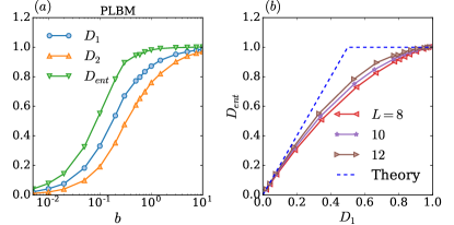
Figure 4: Scaling exponents of EE, $D_{ent}$, Shannon entropy, $D_{1}$, and IPR, $D_{2}$ for PLRBM. (a) $D_{ent}$, $D_{1}$, and $D_{2}$ extracted by linear extrapolation from EE, Shannon entropy $D_{1}\ln N$, and the IPR $D_{2}\ln N$ scalings versus subsystem size $N_{A}=2^{L/2}$.(b) The parametric plot of $D_{ent}$ versus $D_{1}$. Different curves correspond to the different points $L-2$, $L$, $L+2$ of an enlarging linear fitting procedure.

For genuine multifractal states, characterized by non-trivial exponents $D_{q}$, and for $N_{A}=N^{p}$, the upper bound, Eq. (7) rewritten as the lower bound for fractal dimensions $\overline{D_{q}}\ln N\geq\mathcal{S}_{q}(A)$, $q\geq 1$, of a state with fixed Renyi entropies $0\leq\mathcal{S}_{q}(A)\leq\ln N_{A}$ can be proved to be strict and can be saturated by the change of the subsystem bases Bas . Indeed, one can show MF- that the minimal value $D_{q}$ can be achieved if the computational basis is optimized to be the Schmidt decomposition basis $\left|\psi\right\rangle=\sum_{a}\lambda_{M_{a}}^{1/2}\left|M_{a}\right\rangle_{A}\otimes\left|m_{a}\right\rangle_{B}$ as in this case $\psi_{M_{a},m_{a^{\prime}}}=\lambda_{M_{a}}^{1/2}\delta_{a,a^{\prime}}$, see Appendix F.

In order to demonstrate the validity of this general bound in Fig. 12, we show the scaling of the fractal exponents, $D_{1}$ and $D_{2}$ extracted from $\text{IPR}_{q}$, and $D_{ent}$ from EE, for the paradigmatic example of power-law random banded matrices (PLBM) Evers and Mirlin (2008) known to have genuine multifractality of eigestates at the critical point, tuned by the parameter $b$. Plotting $D_{ent}$ versus $D_{1}$, we see that the universal bound is satisfied, though not saturated for the inspected system sizes. We show the results for another exemplary many-body system in Appendix G.

Fluctuations— Quantum fluctuations represent another important ingredient to understand ergodicity. According to ETH, they can be related to temporal fluctuations around the equilibrium value in a quench protocol. In ergodic systems the scaling of fluctuations is related to the dimension of the larger subsystem playing the role of a bath Nadal et al. (2010, 2011); Majumdar (2015); Vivo et al. (2016). EE fluctuations can be quantified by the standard deviation

$$\overline{\delta\mathcal{S}_{1}}(A)=(\overline{\mathcal{S}_{1}^{2}}(A)-\overline{\mathcal{S}_{1}}^{2}(A))^{1/2}\sim N^{-D_{fluc}/2},$$ (8)

from the collapse with $L$ of the probability distribution $\mathcal{P}(x)$ of the rescaled variable $x=(\mathcal{S}(A)-\overline{\mathcal{S}}(A))/{\overline{\delta\mathcal{S}}(A)}$ (see Appendix E). Importantly, the scaling of fluctuations displays three different regimes for a generic cut $N_{A}=N^{p}$, $p\leq 1/2$, (see inset in Fig. 2 for $p=1/2$)

$$D_{fluc}=\left\{\begin{array}[]{ll}D,&D<p\\ 2D-p,&p<D<1-p/2\\ 2(1-p),&D>1-p/2\end{array}\right.\ .$$ (9)

For $D<p$, both mean EE and its fluctuations show the properties of local observables: their scaling is related to the equilibration within the fractal support set $N^{D}$ and does not depend on the subsystem size. For $p<D<1-p/2$ the mean EE saturates at the Page value for the considered subsystem size, Eq. (7), and, thus, for such states EE cannot be considered as a local observable. The fluctuations in this case have fingerprints of a non-ergodic behavior, $\overline{\delta\mathcal{S}}(A)\sim N^{-(2D-p)}$. Finally for $1-p/2<D<1$, both mean and its fluctuations are undistinguishable from ergodic states at infinite temperature .

Conclusions— In order to answer to the main question of the paper – to what extend ergodicity properties extracted from entanglement and multifractal probes provide the same description of thermal phases – we generalized the result of Ref. Page (1993) on the EE for RPS to the case of NEE states characterized by fractal dimensions $D_{q}$. In particular, we presented an upper bound for the entanglement entropies $\mathcal{S}_{q}$ (both von Neumann and Renyi) of a generic multifractal state with fractal dimensions $D_{q}$, see Appendix F.

This bound leaves the gap for $\mathcal{S}_{q}(A)$ to be equal to the Page value provided the wave function support set is larger than the subsystem size, $N^{D_{q}}>N_{A}$. An example of the saturation of this bound is shown for a newly introduced class of sparse random pure states. Our results show that for small fractal dimensions $N^{D_{q}}<N_{A}$ EE behaves as a local observable both in terms of the mean value and fluctuations.

Thus, ergodicity viewed as the wave function equipartition in the full Hilbert space is more strict than the one imposed by the value of the EE.

Our results find immediate application in the many-body localization theory where EE is used to probe the transition, or in strongly kinematically constrained models where ergodicity may break down due to Fock/Hilbert space fragmentation. For instance, in spin models in Refs. Sala et al. (2019); De Tomasi et al. (2019), the eigenstates live on an exponentially small fraction of the full Hilbert, due to dipole conservation Sala et al. (2019); wea and strong interactions De Tomasi et al. (2019) (Fock-space fragmentation). Nevertheless, the half-chain entanglement entropy equals to the Page value, provided the fractal dimension of the wave function support set is $D>1/2$, see Appendix G.

Appendix A Numerical tests of diagonal approximation

In this section, we provide further numerical evidence of the validity of the diagonal approximation. In the main text we used the diagonal approximation $\overline{\mathcal{S}_{1}^{\text{diagonal}}}(A)=-\overline{\sum_{M}\rho_{M,M}^{A}\ln{\rho_{M,M}^{A}}}$ to estimate the scaling of the von Neumann EE $\mathcal{S}_{1}(A)$. Figure 5 show both $\mathcal{S}_{1}(A)$ and $\overline{\mathcal{S}_{1}^{\text{diagonal}}}(A)$ for half-partition $N_{A}=2^{L/2}$, as function of $L$ for several fractal dimension $D$, giving indication that $\overline{\mathcal{S}_{1}}(A)\simeq\overline{\mathcal{S}_{1}^{\text{diagonal}}}(A)$.

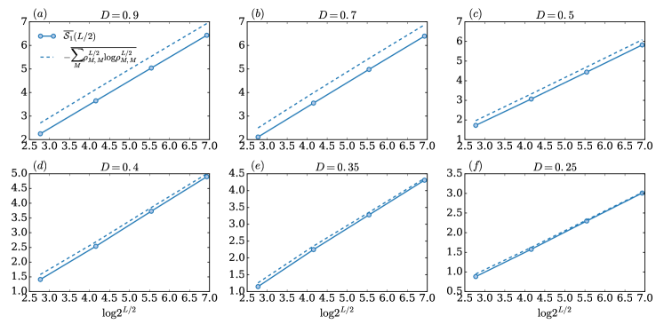
Figure 5: Diagonal approximation and von Neumann EE (a)-(f) half-partition averaged EE $\overline{\mathcal{S}_{1}}(L/2)$ (solid-line) and its diagonal approximation $\overline{\mathcal{S}_{1}^{\text{diagonal}}}(L/2)=-\overline{\sum_{M}\rho_{M,M}^{A}\ln{\rho_{M,M}^{A}}}$ (dashed line) as a function of $L$ for several fractal dimension $D$.

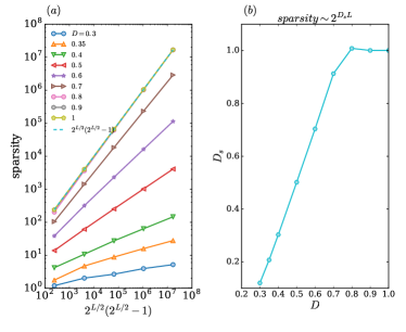
Figure 6: Sparsity of the off-diagonal elements of $\rho_{A}$ for $N_{A}=2^{L/2}$. (a) Sparsity $S$ defined as the number of non-zero off-diagonals in the density matrix as a function of the total number $N_{A}(N_{A}-1)$ of off-diagonals of $\rho_{A}$ at half-partition ($N_{A}=2^{L/2}$) for several $D$. (b) Rate $D_{s}$ of non-zero off-diagonal elements, $S\sim 2^{2pD_{s}L}$ as a function of the fractal dimension $D$.

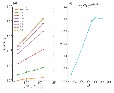
Figure 7: Sparsity of the off-diagonal elements of $\rho_{A}$ for $N_{A}=2^{L/3}$. (a) Sparsity as function of $N_{A}(N_{A}-1)$ for several $D$. (b) Rate $D_{s}$ of non-zero off-diagonal elements, $S\sim 2^{2pD_{s}2L/3}$ as a function of the fractal dimension $D$.

To understand numerically why the diagonal approximation works well, we analyze in more detail the structure of the reduced density matrix $\rho_{A}$. First, we start to investigate the sparse property of $\rho_{A}$. For this purpose, we define the sparsity of $\rho_{A}$ as the number of its non-zero off-diagonal elements, $S=\#\{|\rho_{A}^{M,M^{\prime}}|\neq 0\}$. Figure 6(a) and Fig. 7(a) show the sparsity of $\rho_{A}$ for two different partition $N_{A}=2^{L/2}$ and $N_{A}=2^{L/3}$, respectively. As one can notice, for large $D$ the number of non-zeros in $\rho_{A}$ grows as the total size of the reduced density matrix $N_{A}^{2}$ meaning that the matrix is not sparse for these values of $D$ . Nevertheless, for small $D$, $\rho_{A}$ is sparse and the number of non-zeros elements of $\rho_{A}$ is an exponentially small fraction of the full dimension.

To better quantify the sparsity of $\rho_{A}$, we define the rate $D_{s}$ as $S\sim N^{2D_{s}p}$. For $D_{s}=1$ the matrix is not sparse, and $\rho_{A}$ is diagonal for $D_{s}=0$. Figure 6(b) and Fig. 7(b) show $D_{s}$ for two different partitions $N_{A}=2^{L/2}$ and $N_{A}=2^{L/3}$, respectively. As expected, for large $D$ we have $D_{s}=1$, while $D_{s}$ is proportional to $D$ for smaller $D$. In the next section, we will give an analytical argument showing

$$D_{s}\simeq\left\{\begin{array}[]{ll}\frac{2D-1+p}{2p},&D<\frac{1+p}{2}\\ 1,&D>\frac{1+p}{2}\end{array}\right.\ .$$ (10)

and demonstrate that sparsity plays a major role for the validity of the diagonal approximation.

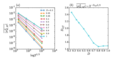
Figure 8: Mean off-diagonal element of $\rho_{A}$ for $N_{A}=2^{L/2}$. (a)  $\overline{|\rho_{M,M^{\prime}}^{A}|}$ as a function of $L$ for several $D$. (b) $D_{off}$ exponent extracted from $\overline{|\rho_{M,M^{\prime}}^{A}|}\sim 2^{-pD_{off}L}$, $p=1/2$ as a function of $D$.

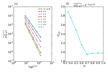
Figure 9: Mean off-diagonal element of $\rho_{A}$ for $N_{A}=2^{L/3}$. (a)  $\overline{|\rho_{M,M^{\prime}}^{A}|}$ as a function of $L$ for several $D$. (b) $D_{off}$ exponent extracted from $\overline{|\rho_{M,M^{\prime}}^{A}|}\sim 2^{-pD_{off}L}$, $p=1/3$ as a function of $D$.

Now, we calculate the mean off-diagonal elements of $\rho_{A}$ (not only non-zero ones). Figure 8 (a) and Fig. 9 (a) show $\overline{|\rho_{M,M^{\prime}}^{A}|}$ as function of $L$ for several $D$ for two different partitions $N_{A}=2^{L/2}$ and $N_{A}=2^{L/3}$, respectively. In general, we have $\overline{|\rho_{M,M^{\prime}}^{A}|}\sim N^{-D_{off}p}$. Figure 8 (b) and Fig. 9 (b) show $D_{off}$ as a function of $D$. In the next section, we will show that

$$pD_{off}\simeq\left\{\begin{array}[]{ll}1+p-D,&D<\frac{1+p}{2}\\ \frac{1+p}{2},&D>\frac{1+p}{2}\end{array}\right.\ .$$ (11)

Appendix B Structure of reduced density matrix

In this section, we consider the structure of diagonal

$$\rho_{M,M}^{A}=\sum_{m=1}^{N_{B}}|\psi_{M,m}|^{2}\ ,$$ (12)

and off-diagonal

$$\rho_{M,M^{\prime}}^{A}=\sum_{m=1}^{N_{B}}\psi_{M,m}\psi^{*}_{M^{\prime},m}\ ,$$ (13)

elements of the reduced density matrix $\rho_{A}$ assuming the vectors $\psi_{M}$ and $\psi_{M^{\prime}}$ to be uncorrelated for $M\neq M^{\prime}$ with a certain probability distribution of each element

$$P(\psi_{M,m})=(1-p_{0})\delta(\psi_{M,m})+\\ p_{0}P_{1}(N^{D/2}\psi_{M,m})N^{D/2}\ .$$ (14)

Here, $p_{0}=N^{D}/N$ is the probability that $\psi_{M,m}\neq 0$. $P_{1}(y)$ is the probability distribution of non-zero values, which is symmetric $P_{1}(-y)=P_{1}(y)$, has a unit variance $\int y^{2}P_{1}(y)dy=1$ and the fourth cumulant $\sigma^{2}=\int(y^{2}-1)^{2}P_{1}(y)dy\sim O(1)$ . The latter conditions ensure the scaling $|\psi_{M,m}|^{2}\sim N^{-D}$ of non-zero elements and the wave function normalization (on average). In the limit of large $N$, we can further neglect the correlations related to the normalization condition.

Next, within the above assumptions one can find the probability distributions of diagonal, Eq. (12), and off-diagonal, Eq. (13), elements of the reduced density matrix (similar to Khaymovich et al. (2019)). For this purpose we rewrite Eq. (14) in a short form for $N^{D/2}\psi_{M,m}=y$

$$P(y)=(1-p_{0})\delta(y)+p_{0}P_{1}(y)\ .$$ (15)

B.1 Probability distribution of diagonals $\rho_{M,M}^{A}$

Here we use the Fourier transform to calculate the $N_{B}$-fold convolution of the probability distribution $\tilde{P}_{1}(t^{\prime})=\frac{P_{1}\left(\sqrt{t^{\prime}}\right)}{\sqrt{t^{\prime}}}$ of $t^{\prime}=|\psi_{M,m}|^{2}$ and obtain

$$P(\rho_{M,M}^{A})=\sum_{k=0}^{N_{B}}\left(N_{B}\atop k\right)(1-p)^{N_{B}-k}p^{k}\tilde{P}_{k}(\rho_{M,M}^{A}N^{D})\ ,$$ (16)

with

$$\tilde{P}_{k}(t)=\frac{1}{2\pi}\int e^{-i\omega t}\left(\int\frac{P_{1}\left(\sqrt{t^{\prime}}\right)}{\sqrt{t^{\prime}}}e^{i\omega t^{\prime}}\right)^{k}d\omega\ .$$ (17)

The scaling of $p_{0}=N^{D-1}$ and $N_{B}=N^{1-p}$ provide the optimal index

$$k_{*}=N_{B}p_{0}=N^{D-p}$$ (18)

giving the main contribution to the sum Eq. (16).

As $k$ is integer, one has to distinguish two cases: (i) $D<p$ when $k_{*}=N_{B}p_{0}\ll 1$ and, thus, the probability distribution is nearly bimodal

$$P(\rho_{M,M}^{A}=x)dx\simeq(1-k_{*})\delta(x)dx+k_{*}\tilde{P}_{1}(N^{D}x)N^{D}dx\ ,$$ (19)

and (ii) $D>p$ when $k_{*}=N_{B}p_{0}\gg 1$ and the central limit theorem (CLT) works giving

$$P(\rho_{M,M}^{A})=\frac{e^{-(\rho_{M,M}^{A}-N^{-p})^{2}/(2\sigma^{2}N^{-D-p})}}{\sqrt{2\sigma^{2}N^{-D-p}}}\ .$$ (20)

This analysis shows that for $D>p$ the diagonal $\rho_{A}$-elements are homogeneously distributed with the mean value $\rho_{M,M}^{A}=1/N_{A}$ given by $\text{Tr}[\rho_{A}]=1$.

B.2 Probability distribution of off-diagonals $\rho_{M,M^{\prime}}^{A}$

To obtain $P(\rho_{M,M^{\prime}}^{A})$ one has to calculate, first, from Eq. (15)

$$P(N^{D}\psi\psi^{\prime}=z)=\iint P(y)P(y^{\prime})\delta(z-yy^{\prime})dydy^{\prime}\\ =(1-p^{2})\delta(z)+p_{0}^{2}\bar{P}(z)\ ,$$ (21)

with

$$\bar{P}_{1}(z)=\iint P_{1}(y)P_{1}(y^{\prime})\delta(z-yy^{\prime})dydy^{\prime}\ .$$ (22)

Then, analogously to the previous subsection, one can use the Fourier transform to calculate

$$P(\rho_{M,M^{\prime}}^{A})=\sum_{l=0}^{N_{B}}\left(N_{B}\atop l\right)(1-p_{0}^{2})^{N_{B}-l}p_{0}^{2l}\bar{P}_{l}(\rho_{M,M}^{A}N^{D})\ ,$$ (23)

with

$$\bar{P}_{l}(t)=\frac{1}{2\pi}\int e^{-i\omega t}\left(\int\bar{P}_{1}\left(z^{\prime}\right)e^{i\omega z^{\prime}}\right)^{l}d\omega\ .$$ (24)

The scaling of $p_{0}=N^{D-1}$ and $N_{B}=N^{1-p}$ provide the optimal index

$$l_{*}=N_{B}p_{0}^{2}=N^{2D-1-p}$$ (25)

giving the main contribution to the sum Eq. (23).

As $l$ is integer, one has to distinguish two cases: (i) $D<\frac{1+p}{2}$ when $l_{*}=N_{B}p_{0}^{2}\ll 1$ and, thus, the probability distribution is nearly bimodal

$$P(\rho_{M,M^{\prime}}^{A}=x)dx\simeq(1-l_{*})\delta(x)dx+\\ l_{*}\bar{P}_{1}(N^{D}x)N^{D}dx\ ,$$ (26)

and (ii) $D>\frac{1+p}{2}$ when $l_{*}=N_{B}p_{0}^{2}\gg 1$ and CLT works giving

$$P(\rho_{M,M^{\prime}}^{A})=\frac{e^{-(\rho_{M,M^{\prime}}^{A})^{2}/(2\sigma^{2}N^{-1-p})}}{\sqrt{2\sigma^{2}N^{-1-p}}}\ .$$ (27)

Here we used the fact that $\bar{P}_{1}(z)=\bar{P}_{1}(-z)$ is symmetric and thus there is no drift in CLT.

The latter analysis confirms the scaling of the off-diagonal elements, Eq. (11), as well as the number of non-zero off-diagonals, Eq. (10). Indeed, for $D>\frac{1+p}{2}$ the distribution is smooth with the typical value

$$\rho_{M,M^{\prime}}^{A}\sim N^{-\frac{1+p}{2}}\ ,$$ (28)

thus, the rate of non-zero off-diagonal elements $D_{s}=1$ and their scaling $\overline{|\rho_{M,M^{\prime}}^{A}|}\sim 2^{-pD_{off}L}$ is $D_{off}=\frac{1+p}{2p}$.

In the opposite limit of $D<\frac{1+p}{2}$ the distribution is bimodal giving the number of non-zeros

$$N^{2pD_{s}}=N_{A}^{2}l_{*}=N^{2D-1+p}$$ (29)

as well as the mean value

$$\overline{|\rho_{M,M^{\prime}}^{A}|}=N^{-pD_{off}}=l_{*}N^{-D}=N^{D-1-p}\ .$$ (30)

Appendix C Sparseness of the reduced density matrix for non-ergodic states

Now, we provide an analytical argument to support the validity of the diagonal approximation in the regime in which $\rho_{A}$ is sparse. As we are interested in the scaling of the Schmidt values with $N$ compared to the one of diagonal elements $\rho_{M,M}^{A}$, we have to consider two cases: (i) First, when the number of non-zero elements in each row is finite and does not grow with $N$, the off-diagonal elements can be of the same order as the diagonal ones. (ii) Second, when there are many non-zero off-diagonals which are much smaller than $\rho_{M,M}^{A}$.

C.1 Few non-zero off-diagonal elements $\rho_{M,M^{\prime}}^{A}$, ($D<1/2$)

As follows from Eq. (10) there is at most $O(1)$ non-zero off-diagonal elements in each row as soon as $D<1/2$ (the total number of off-diagonals $\sim N_{A}$).

In this case, we can show that in terms of multifractal scaling with the total Hilbert space dimension $N$ in the above regime the Schmidt values $\lambda_{M}$ scale in the same way as the diagonal elements of $\rho_{A}$ and, thus, EE can be approximated by its diagonal counterpart Polkovnikov (2011); Santos et al. (2011)

$$\mathcal{S}_{q}(p)=\frac{\ln\Sigma_{q}}{1-q},\quad\Sigma_{q}=\sum_{M}\lambda_{M}^{q}\simeq\sum_{M}\left(\rho^{A}_{M,M}\right)^{q}\ .$$ (31)

Indeed, if in each row of $\rho_{A}$ there are only few significantly non-zero off-diagonal matrix elements (say, for $M$th and $M^{\prime}$th diagonals), then Schmidt eigenvalues can be approximated by diagonalizing a $2$-by-$2$ matrix

$$\left(\begin{array}[]{cc}\rho^{A}_{M,M}&\rho^{A}_{M,M^{\prime}}\\ \rho^{A}_{M^{\prime},M}&\rho^{A}_{M^{\prime},M^{\prime}}\\ \end{array}\right)\ .$$ (32)

Assuming the following scaling $\rho^{A}_{M,M}\sim N^{-\alpha_{M}}$, and $\rho^{A}_{M,M^{\prime}}\sim N^{-\beta}$, with $\alpha_{M}\leq\alpha_{M^{\prime}}$ without loss of generality, we obtain for the corresponding Schmidt values

$$\lambda_{M/M^{\prime}}=\frac{N^{-\alpha_{M}}+N^{-\alpha_{M^{\prime}}}\pm\sqrt{\left(N^{-\alpha_{M}}+N^{-\alpha_{M^{\prime}}}\right)^{2}+4N^{-2\beta}}}{2}\simeq\\ \left\{N^{-\alpha_{M}}+N^{-2\beta+\alpha_{M}}\simeq N^{-\alpha_{M}}\atop N^{-\alpha_{M^{\prime}}}+N^{-2\beta+\alpha_{M}}\simeq N^{-\alpha_{M^{\prime}}}\right.\ .$$ (33)

The latter approximation is based on the inequality $\beta\geq(\alpha_{M}+\alpha_{M^{\prime}})/2$ leading from the Cauchy-Bunyakovski-Schwarz inequality for the off-diagonal element by the geometric mean of diagonals

$$\left|\rho^{A}_{M,M^{\prime}}\right|=\left|\sum_{m=1}^{N_{B}}\psi_{M,m}\psi_{M^{\prime},m}^{*}\right|\leq\\ \sqrt{\sum_{m=1}^{N_{B}}\left|\psi_{M,m}\right|^{2}\sum_{m^{\prime}=0}^{N_{B}}\left|\psi_{M^{\prime},m^{\prime}}\right|^{2}}=\sqrt{\rho^{A}_{M,M}\rho^{A}_{M^{\prime},M^{\prime}}}\ .$$ (34)

As a result, the scaling of Schmidt values $\lambda_{M}$ with $N$ is shown to be the same as for the diagonal elements $\rho^{A}_{M,M}$ in the nearly diagonal sparse regime of $\rho_{A}$ ($D<1/2$). In next sections we will use this fact to calculate the Renyi and entanglement entropies.

C.2 Many non-zero off-diagonal elements $\rho_{M,M^{\prime}}^{A}$, ($D>1/2$)

In the case of $D>1/2$ there is an extensive number of non-zero off-diagonal elements of the reduced density matrix. In order to estimate them we assume their statistical independence from each other and from the diagonal elements following the case $D=1$ considered in Vivo et al. (2016).

In the case of $D>\frac{1+p}{2}>p$ both diagonal and off-diagonal elements of the reduced density matrix are homogeneously distributed and the latter has the form similar to the Rosenzweig-Porter random matrix ensemble Rosenzweig and Porter (1960). Then the Schmidt eigenspectrum is not affected by the off-diagonal elements when Kunz and Shapiro (1998)

$$\frac{|\rho_{M,M^{\prime}}^{A}|}{\rho_{M,M}^{A}}\sim N^{-\frac{1-p}{2}}\ll N^{-p/2}\ ,$$ (35)

which is the case as $p\leq 1/2$.

In general for $D>1/2$ one can apply the Mott’s principle of delocalization Mott (1966) recently generalized in Nosov et al. (2019) which reads for $N_{A}\times N_{A}$ matrix, $N_{A}=N^{p}$, as follows: the spectrum is not affected by the off-diagonal elements as soon as

$$N^{p}\frac{\overline{|\rho_{M,M^{\prime}}^{A}|^{2}}}{\overline{|\rho_{M,M}^{A}|^{2}}}\ll 1\ .$$ (36)

In our case it leads to

$$N^{p}\frac{\overline{|\rho_{M,M^{\prime}}^{A}|^{2}}}{\overline{|\rho_{M,M}^{A}|^{2}}}\sim\left\{\begin{array}[]{ll}N^{2D-2+p},&D<\frac{1+p}{2}\\ N^{2p-1},&D>\frac{1+p}{2}\end{array}\right.\ ,$$ (37)

and works for any $0\leq D\leq 1$.

Appendix D Entanglement entropy for fractal states

In this section, we consider mean and fluctuations of Renyi and von Neumann EE within the approximations of two previous sections.

The simplest way to calculate the Renyi entropy, Eq. (31), in the diagonal approximation

$$\lambda_{M}\simeq\rho^{A}_{M,M}=\sum_{m=1}^{N_{B}}\left|\psi_{M,m}\right|^{2}$$ (38)

is to use the probability distributions, Eq. (19), and, Eq. (20). Indeed,

$$\overline{\Sigma_{q}}=N_{A}\overline{\left(\rho_{M,M}^{A}\right)^{q}}=\left\{\begin{array}[]{ll}N^{D(1-q)},&D<p\\ N^{p(1-q)},&D>p\end{array}\right.\ ,$$ (39)

leading straightforwardly to Eq. (8) of the main text.

The fluctuations can be also estimates from the moments as soon as the variance

$$\sigma_{\Sigma}^{2}=\overline{\Sigma_{q}^{2}}-\overline{\Sigma_{q}}^{2}=N_{A}\left[\overline{\left(\rho_{M,M}^{A}\right)^{2q}}-\overline{\left(\rho_{M,M}^{A}\right)^{q}}^{2}\right]$$ (40)

is small compared to $\overline{\Sigma_{q}}^{2}$. Indeed, as

$$(1-q)\mathcal{S}_{q}(p)=\ln\Sigma_{q}=\ln\overline{\Sigma_{q}}+\ln\left[1+\frac{\sigma_{\Sigma}}{\overline{\Sigma_{q}}}g_{q}\right]\simeq\\ \ln\overline{\Sigma_{q}}+\frac{\sigma_{\Sigma}}{\overline{\Sigma_{q}}}g_{q}-\frac{\sigma_{\Sigma}^{2}}{2\overline{\Sigma_{q}}^{2}}g_{q}^{2}\$$ (41)

it gives

$$(1-q)\overline{\mathcal{S}_{q}(p)}=\ln\overline{\Sigma_{q}}-\frac{\sigma_{\Sigma}^{2}}{2\overline{\Sigma_{q}}^{2}}\simeq\ln\overline{\Sigma_{q}}$$ (42)

within the leading approximation, and

$$(1-q)^{2}\left[\overline{\mathcal{S}_{q}^{2}(p)}-\overline{\mathcal{S}_{q}(p)}^{2}\right]=\frac{\sigma_{\Sigma}^{2}}{\overline{\Sigma_{q}}^{2}}\ .$$ (43)

Here we introduced dimensionless variable $g_{q}=\frac{\Sigma_{q}-\overline{\Sigma_{q}}}{\sigma_{\Sigma}}$ with zero mean and unit variance

$$\overline{g_{q}}=0\ ,\quad\overline{g_{q}^{2}}=1\ .$$ (44)

In our case one obtains

$$\frac{\sigma_{\Sigma}^{2}}{\overline{\Sigma_{q}}^{2}}=N^{-D}\ ,$$ (45)

giving the correct approximation for $D<p$.

D.1 Alternative way to calculate entanglement entropies

Alternatively in the main text we parameterize Schmidt values as follows

$$\lambda_{M}\simeq\rho^{A}_{M,M}=\sum_{m=1}^{N_{B}}\left|\psi_{M,m}\right|^{2}=g_{M}/N^{D}\ ,$$ (46)

where $0\leq g_{M}\leq N^{D}$ are integer values summed to the support set $N^{D}$:

$$\sum_{M=1}^{N_{A}}g_{M}=N^{D}\ .$$ (47)

The entanglement entropy in this case can be estimated as the logarithm of the number $N_{0}$ of non-zero $g_{M}$

$${\mathcal{S}}_{1}\sim\ln N_{0}\ .$$ (48)

As we show below, this approximation is good for mean EE for any $D$, but fails to capture fluctuations for $D>p$.

The probability distribution $P_{N_{0}}$ of $N_{0}$ can be calculated combinatorically in the assumption of homogeneous distribution of $g_{M}$’s. Indeed, the total number of combinations of $N_{A}$ values of $g_{M}$, $1\leq M\leq N_{A}$, taken with repetitions ($g_{M}$ can be larger than $1$) and with the normalization Eq. (47) is given by

$${\mathcal{M}}=\left(N_{A}+N^{D}-1\atop N^{D}\right)\ .$$ (49)

At the same time the combinations with $N_{0}$ non-zero $g_{M}$ can be counted as the number of combination to realize $N_{0}$ non-zeros

$${\mathcal{M}}_{\bar{0}}=\left(N^{D}-1\atop N_{0}-1\right)$$ (50)

times the number of combinations to place them among $N_{A}$, which is

$${\mathcal{M}}_{N_{0}}=\left(N_{A}\atop N_{0}\right)\ .$$ (51)

As a result

$$P_{N_{0}}=\frac{{\mathcal{M}}_{\bar{0}}{\mathcal{M}}_{N_{0}}}{{\mathcal{M}}}\simeq A(N)e^{N_{A}f(\rho)}\ ,$$ (52)

where

$$f(\rho,\alpha)=-2\rho\ln(\rho)-(\alpha-\rho)\ln(\alpha-\rho)-(1-\rho)\ln(1-\rho)\ ,$$ (53)

$N^{D}=\alpha N_{A}$, and $0\leq\rho=N_{0}/N_{A}\leq 1,\alpha$ and we neglected $-1$ comparing both to $N^{D}$ and $N_{0}$. The expression for $f(\rho)$ is calculated in the large-$N$ limit with help of Stirling’s approximation.

The maximum of $f(\rho)$ is achieved at the typical $N_{0}^{*}=N_{A}\rho^{*}$ with

$$~{}\rho^{*}=\frac{\alpha}{1+\alpha}<1,\alpha\text{ leading to }N_{0}^{*}=\frac{N_{A}N^{D}}{N_{A}+N^{D}}\$$ (54)

from the main text.

The relative fluctuations $\delta N_{0}/{N_{0}^{*}}=\delta\rho/{\rho^{*}}$ can be written in the following form

$$\frac{\delta N_{0}}{N_{0}^{*}}=\frac{\delta\rho_{0}}{\rho_{0}^{*}}=\frac{1}{\sqrt{-N_{A}f^{\prime\prime}(\rho^{*})}\rho_{0}^{*}}=\left(N_{A}+N^{D}\right)^{-1/2}\$$ (55)

in the Gaussian approximation

$$P_{N_{0}}=\frac{e^{-(N_{A}+N^{D})(\rho-\rho^{*})^{2}/2}}{\sqrt{2\pi/(N_{A}+N^{D})}}\ ,$$ (56)

derived from Eq. (52) and Eq. (53) provided $\rho^{*}\gg(N_{A}+N^{D})^{-1/2}$.

In the same approximation

$$\overline{\ln N_{0}}=\ln N_{0}^{*}-\frac{1}{2(N_{A}+N^{D})},$$ (57a)

$$\overline{\ln^{2}N_{0}}=\ln^{2}N_{0}^{*}+\frac{1-\ln N_{0}^{*}}{(N_{A}+N^{D})}\ .$$ (57b)

According to Eq. (48) and Eq. (57a) mean EE is given by

$$\overline{\mathcal{S}_{1}}\simeq\overline{\ln N_{0}}=\ln N_{0}^{*}-\frac{1}{2(N^{D}+N_{A})}\\ \sim\left\{\ln N^{D}=D\ln N,\text{ for }D_{1}<p\atop\ln N_{A}=p\ln N,\text{ for }D_{1}>p\right.\ .$$ (58)

In the latter equality we neglected subleading terms.

At the same time according to Eq. (57a) and Eq. (57b) EE fluctuations are given mostly by the relative fluctuations of $N_{0}$

$$\overline{\mathcal{S}_{1}^{2}}-\overline{\mathcal{S}_{1}}^{2}\simeq\overline{\ln^{2}(N_{0})}-\overline{\ln(N_{0})}^{2}\simeq\frac{1}{N^{D}+N_{A}}\ .$$ (59)

As mentioned above the approximation Eq. (48) works both for the mean and fluctuations provided $D<p$. This is the case as well for all Renyi entropies. It is caused by the fact that $N_{0}\simeq N^{D}$ and, thus, all $g_{M}\sim O(1)$ leading to

$$\overline{\Sigma_{q}}=\sum_{M}\overline{\lambda_{M}^{q}}=\sum_{M}\overline{\left(\frac{g_{M}}{N^{D}}\right)^{q}}\sim N_{0}N^{-Dq}=N^{D(1-q)}$$ (60)

and

$$\overline{\Sigma_{q}^{2}}-\overline{\Sigma_{q}}^{2}=\sum_{M}\overline{\left(\frac{g_{M}}{N^{D}}\right)^{2q}}-\overline{\left(\frac{g_{M}}{N^{D}}\right)^{q}}^{2}\sim N^{D(1-2q)}\ .$$ (61)

However, in the opposite case $D>p$ when $N_{0}\simeq N_{A}\ll N^{D}$ there is a non-trivial distribution of $g_{M}$ with $\overline{g_{M}}=N^{D}/N_{A}\gg 1$ and

$$\ln N_{0}\neq\frac{\ln\left[\sum_{M}\left(\frac{g_{M}}{N^{D}}\right)^{q}\right]}{1-q}\ .$$ (62)

Nevertheless, as we have shown in Sec. A, on average both sides of the latter equation give the same Page value as Eq. (8) in the main text.

Appendix E Collapse of the EE probability distribution for S-RPS

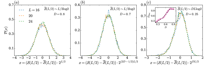
Figure 10: Collapse of the probability distribution $\mathcal{P}(x)$ of the half-system EE at finite sizes $L$, $x=(\mathcal{S}-\overline{\mathcal{S}})/{\overline{\delta\mathcal{S}}}$, for different $D$: (a) $D=0.8$, (b) $D=0.7$, (c) $D=0.25$. Scaling of the mean EE, $\overline{\mathcal{S}_{1}}(A)$, is shown in the legend, while the distribution width scaling is specified in the axis label. (inset) Slope $D_{fluc}$ of the standard deviation $\overline{\delta\mathcal{S}}(L/2)\sim D_{fluc}\ln{2^{L/2}}$ versus $D$. Black dashed line shows analytical prediction, Eq. (64), for $p=1/2$.

Here, we numerically characterize EE fluctuations for the S-RPS. EE fluctuations can be quantified by the standard deviation

$$\overline{\delta\mathcal{S}_{1}}(A)=(\overline{\mathcal{S}_{1}^{2}}(A)-\overline{\mathcal{S}_{1}}^{2}(A))^{1/2}\sim N^{-D_{fluc}/2},$$ (63)

from the collapse with $L$ of the probability distribution $\mathcal{P}(x)$ of the rescaled variable $x=(\mathcal{S}(A)-\overline{\mathcal{S}}(A))/{\overline{\delta\mathcal{S}}(A)}$. Figure 10 shows the collapse of $\mathcal{P}(x)$ with $L$ for S-RPS for several $D$ and $N_{A}=2^{L/2}$. Scaling of fluctuations extracted from the above collapse displays three different kinds of behavior for a generic cut $N_{A}=N^{p}$, $p\leq 1/2$, (see inset in Fig. 10 for $p=1/2$)

$$D_{fluc}=\left\{\begin{array}[]{ll}D,&D<p\\ 2D-p,&p<D<1-p/2\\ 2(1-p),&D>1-p/2\end{array}\right.\ .$$ (64)

For $D<p$, both mean EE and its fluctuations show the properties of local observables: their scaling is related to the equilibration within the fractal support set $N^{D}$ and does not depend on the subsystem size – and correspond to the analytical results of the previous section. For $p<D<1-p/2$ the mean EE saturates at the Page value for the considered subsystem size, Eq. (58), and, thus, for such states EE cannot be considered as a local observable. The fluctuations in this case have fingerprints of a non-ergodic behavior, $\overline{\delta\mathcal{S}}(A)\sim N^{-(2D-p)}$. Finally for $1-p/2<D<1$, both mean and its fluctuations are undistinguishable from ergodic states at infinite temperature.

Appendix F Upper bound for the mean entanglement entropy for multifractal states

For genuine multifractal states the above mentioned derivations are not applicable as its probability distribution is not bimodal like in Eq. (14) or Eq. (15). Thus, in order to proceed we use another approach and show that there is a generic upper bound for the mean Renyi entanglement entropy $\overline{\mathcal{S}_{q}}(A)$ for a state with certain fractal dimensions $0\leq D_{q}\leq 1$

$$\overline{\mathcal{S}_{q}}(A)\leq\left\{\begin{array}[]{ll}D_{q}\ln N,&D_{q}<p\\ \ln N_{A},&D_{q}>p\end{array}\right.\$$ (65)

or vice-a-versa there is a generic lower bound for the fractal dimensions $\overline{D_{q}}$ for a state with certain fixed Renyi entropies $0\leq\mathcal{S}_{q}(A)\leq\ln N_{A}$

$$\overline{D_{q}}\geq\frac{\mathcal{S}_{q}(A)}{\ln N}\ .$$ (66)

Here and further, we restrict our consideration to the physically relevant moments $q\geq 1$.

One should note that both EE and IPR are strongly basis-dependent, thus, generic many-body states may present any point under (above) the found upper (lower) bound. Indeed, one can see it simply by either changing the partition spatial structure (which changes only $\mathcal{S}_{q}(A)$, but not $D_{q}$) or by basis transformations of subsystems (which changes only $D_{q}$, but not $\mathcal{S}_{q}(A)$).

As both Eq. (65) and (66) are equivalent, let’s prove the second one. For this we consider the state

$$\left|\psi\right\rangle=\sum_{a}\lambda_{\alpha}^{1/2}\left|E_{\alpha}\right\rangle_{A}\otimes\left|\varepsilon_{\alpha}\right\rangle_{B}$$ (67)

written in the Schmidt decomposition basis, where $\lambda_{\alpha}$ are (non-zero) Schmidt eigenvalues and $\left|E_{\alpha}\right\rangle_{A}$ and $\left|\varepsilon_{\alpha}\right\rangle_{B}$ are the corresponding eigenvectors in subsystems A and B. From Eq. (31) the $q$th Renyi entropy is given by

$$\mathcal{S}_{q}(A)=\frac{\ln\left[\sum_{M}\lambda_{M}^{q}\right]}{1-q}\$$ (68)

and does not depend on the eigenvectors $\left|E_{\alpha}\right\rangle_{A}$ and $\left|\varepsilon_{\alpha}\right\rangle_{B}$.

On the other hand, the coefficients $\psi_{M,m}$ of $\left|\psi\right\rangle$ in the computational basis $\left|M\right\rangle_{A}\otimes\left|m\right\rangle_{B}$ are highly sensitive to these vectors

$$\psi_{M,m}=\sum_{a}\lambda_{\alpha}^{1/2}\left\langle M|E_{\alpha}\right\rangle_{A}\left\langle m|\varepsilon_{\alpha}\right\rangle_{B}\ ,$$ (69)

so are the fractal dimensions $D_{q}$, Eq. (4)

$${\rm IPR}_{q}\equiv N^{-D_{q}(q-1)}=\sum_{M,m}|\psi_{M,m}|^{2q}\ .$$ (70)

The minimization of $D_{q}$ is equivalent to the maximization of the corresponding IPR. Due to $q>1$ the latter always increases if one replaces several squared coefficients $|\psi_{M,m}|^{2}$ by their squared sum due to the generalized Cauchy-Bunyakovski-Schwarz inequality

$$a^{q}+b^{q}<(a+b)^{q}\ ,\quad a,b>0\ .$$ (71)

This process is equivalent to the change of the computational basis with respect to the Schmidt basis and is limited by the fixed Schmidt eigenvalues.

The maximal value of the IPR_q corresponds to the choice of the computational basis to be the same as the Schmidt eigenbasis

$$\left|M\right\rangle=\left|E_{M}\right\rangle,\quad\left|m\right\rangle=\left|\varepsilon_{m}\right\rangle\ .$$ (72)

and leads to the diagonal reduced density matrix.

The latter gives immediately

$$\psi_{M,m}=\lambda_{M}^{1/2}\delta_{M,m}$$ (73)

and

$$N^{-D_{q}(q-1)}=\sum_{M,m}|\psi_{M,m}|^{2q}=\sum_{M}\lambda_{M}^{q}=e^{-\mathcal{S}_{q}(q-1)}\ .$$ (74)

This concludes the proof of the inequality (66) as in all steps we have just increased the IPR, i.e., decreased $D_{q}$.

Thus, in a general case of a genuine many-body multifractal state, the inequalities (65) and (66) are valid, however their saturation to equalities is an open and difficult question needed further investigations.

In the main text we have provided an example of S-RPS saturating this bound. Here as a counterexample let’s consider fractal NEE states with the structure of the wave function forming a so-called ergodic bubble De Roeck and Huveneers (2017); Luitz et al. (2017); Thiery et al. (2017, 2018); Goremykina et al. (2019); Dumitrescu et al. (2019). Let’s consider the states with only $N^{D}$ non-zero elements, which are Gaussian distributed with the width controlled by the normalization, but unlike S-RPS the distribution of these coefficients will be different. We associate each configuration among $N=2^{L}$ ones with the state of $L$ spins-$1/2$ and assume $DL$ to be an integer number. Then by the ergodic-bubble structure we would mean that for the randomly chosen $DL$ spins from $L$ the wave-function coefficients are non-zero for all the $2^{DL}$ configurations of the selected spins, while the rest $(1-D)L$ spins are frozen in a fixed state.

It is easy to show that as soon as $DL$ spins are chosen randomly among the subsystems A (with $pL$ spins) and B (with $(1-p)L$ spins) the fraction of the chosen spins in the subsystem A is the same as in the total system and equal to $D$. As a result, the reduced density matrix in the subsystem A is represented by the product state of $\sim(1-D)pL$ spins and an ergodic bubble of the size $\sim DpL$. The resulting entanglement entropy is equal to

$$\mathcal{S}_{q}^{\rm bubble}(A)=D\ln N_{A}\ ,$$ (75)

which saturates the bound (65) only in the trivial cases $D=0$ and $D=1$.

Appendix G Further numerical examples

In this section we provide two additional examples of the random matrix and many-body models confirming the general results for the upper bound of EE, Eq. (8) of the main text, and the possibility of EE to be saturated at the Page value for strictly non-ergodic wave functions with $D_{1}<1$.

G.1 Power-law random banded matrix

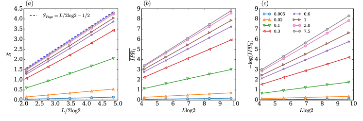
Figure 11: Scaling of EE, Shannon entropy $D_{1}\ln N$, and the logarithm of IPR $D_{2}\ln N$ as a function of subsystem size $N_{A}=2^{L/2}$ for PLRBM at the critical point, $\alpha=1$ for different multifractal parameter $b$. (a) Scaling of the mean von Neumann entanglement entropy $\overline{\mathcal{S}_{1}}(L/2)$ of half-system, $N_{A}=N^{1/2}=2^{L/2}$, as a function of $L$ . Dashed line stands for the Page value scaling; (b) The mean Shannon entropy $\overline{D_{1}}\ln N$ versus $L$; (c) The mean IPR fractal dimension $\overline{D_{2}}\ln N=\ln IPR_{2}$ versus $L$. Values of the multifractal parameter $b$ for all three panels are shown in the legend of panel (c).

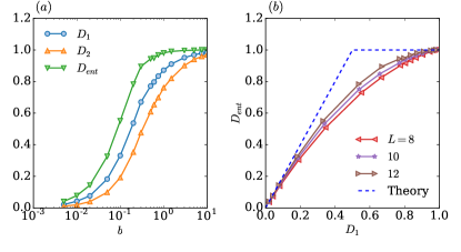
Figure 12: Scaling exponents of EE, $D_{ent}$, Shannon entropy, $D_{1}$, and IPR, $D_{2}$. (a) $D_{ent}$, $D_{1}$, and $D_{2}$ extracted from Fig. 11 by linear extrapolation. (b) The parametric plot of $D_{ent}$ versus $D_{1}$. Different curves correspond to the different points $L-2$, $L$, $L+2$ of an enlarging linear fitting procedure.

In this section, we focus on entanglement properties of the power-law random banded matrix (PLRBM) ensemble Evers and Mirlin (2008) and their relations with the fractal exponents. The PLRBM are defined by

$${\widehat{H}}=\sum_{x,y}^{2^{L}}h_{x,y}|x\rangle\langle y|,$$ (76)

where $h_{x,y}=\mu_{x,y}/(1+(|x-y|/b)^{2\alpha})^{1/2}$ and $\mu_{x,y}=\mu_{y,x}$ are independent random variables uniformly distributed in the interval $[-1,1]$. We consider the case in which the eigenstates of ${\widehat{H}}$ are multifractal, therefore we fix the parameter $\alpha$ to its critical value at the Anderson localization transition (ALT) $\alpha=1$ . The parameter $b$ tunes the multifractal properties of the PLRBM. For $b\gg 1$ the system is weakly multifractal, meaning that $1-D_{1}\propto b^{-1}$ and for $b\ll 1$ it is in a regime of strong multifractality, $D_{1}\propto b$ Evers and Mirlin (2008); Mirlin et al. (1996); Mirlin and Evers (2000); Mirlin and Fyodorov (1993). ${\widehat{H}}$ is defined in a Hilbert space of the dimension $2^{L}$, thus the states $|x\rangle$ could be represented in terms of spin-$1/2$ configurations if one writes them in a binary representation.

Figure 11 (a) shows the bipartite entanglement entropy $\mathcal{S}$ with the subsystem Hilbert space dimension $N_{A}=2^{L/2}$ as a function of $L$ for several $b$. We averaged $\mathcal{S}$ over random configurations, few eigenstates in the middle of the spectrum of ${\widehat{H}}$ and random partitions. As expected for large $b$, we have $\mathcal{S}\simeq\mathcal{S}_{Page}=L/2\log{2}-1/2$. As the parameter $b$ decreases, $\mathcal{S}$ scales still with a volume law, but for $b\lesssim 0.6$ it scales slower than $S_{Page}$, meaning $\overline{\mathcal{S}}\sim D_{ent}L/2\log{2}$ with $D_{ent}<1$. Figures 11 (b)-(c) show the fractal dimensions $\overline{D_{1}}$ and $\overline{D_{2}}$ corresponding to the Shannon entropy and the logarithm of the IPR versus $L$ for several $b$. Usually, the computation of fractal exponents $D_{q}$ is a challenging task and in principle they could have severe finite-size effects (see, e.g., hot debates on the existence of the non-ergodic extended phase in the Anderson model on the random regular graph).

We estimate the three exponents $D_{ent}$, $D_{1}$ and $D_{2}$ by a linear fit repeating Fig. 4 of the main text as Fig. 12. First, Fig. 12 (a) gives numerical evidence of the existence of a genuine multifractal phase, meaning that $D_{q}$ is a non-trivial function of $q$ as $D_{2}<D_{1}$. Second, as one can notice, there is a regime in $b$ for which $D_{ent}\approx 1$, even tough $D_{1}<1$. To understand the finite-size effects for $D_{ent}$ and $D_{1}$, we use an enlarging linear fitting procedure. This means that we compute $D_{1}$ and $D_{ent}$ fitting three consecutive system sizes $\{L-2,L,L+2\}$. Figure 12 (b) shows the result of such fitting $D_{ent}$ as function of $D_{1}$ for several $L$. As expected, $D_{ent}$ obeys the upper-bound that we provided in the main text (dashed line in Fig. 12 (b)). Moreover, the finite-size flow direction suggests that the upper-bound might be saturated in the thermodynamic limit ($L\rightarrow\infty$).

G.2 A quantum many-body system

In conclusion on the main text, we claimed that the results for $D_{ent}$ find an immediate applications for quantum system where Fock/Hilbert space fragmentation take place. In this section, we will give a numerical example for the later model.

We study the $t{-}V$ disordered chain of spinless fermions with periodic boundary conditions,

$${\widehat{H}}=-t\sum_{x}{\widehat{c}}_{x+1}^{\dagger}{\widehat{c}}_{x}+\textit{h.c.}+W\sum_{x}\mu_{x}{\widehat{n}}_{x}+V\sum_{x}{\widehat{n}}_{x}{\widehat{n}}_{x+1},$$ (77)

where ${\widehat{c}}^{\dagger}_{x}$ (${\widehat{c}}_{x}$) is the fermionic creation (annihilation) operator at site $x$, ${\widehat{n}}_{x}={\widehat{c}}_{x}^{\dagger}{\widehat{c}}_{x}$, and $\mu_{x}$ are independent random variables uniformly distributed in the interval $[-1,1]$. $t=1/2$, $W\textsection$ and $V$ are the hopping, disorder and interaction strengths respectively. $L$ is the number of sites and we consider the system at half-filling, i.e. the number of particles is $n=\sum_{x}n_{x}=L/2$. This model is equivalent to the disordered XXZ Heisenberg spin-$1/2$ chain where the interaction $V$ corresponds to the anisotropy along and perpendicular to the $z$-axis.

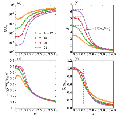
Figure 13: IPR and EE for the many-body model with Hilbert space fragmentation as functions of disorder amplitude $W$. (a) IPR versus $W$ for different system sizes (shown in legend); (b) EE $\overline{\mathcal{S}}$ versus $W$ for the same system sizes. Dashed horizontal lines show the Page value for the corresponding system size; (c) Finite-size estimate $-\log\overline{IPR}/\log\mathcal{N}$ of the fractal dimension $D_{2}$ versus $W$; (d) Finite-size flow of the $\overline{\mathcal{S}}/{\mathcal{S}}_{Page}$. In panels (c) and (d) vertical dashed lines correspond to the $D_{2}(L_{\max})=0.5$, where $L_{\max}=24$ is the maximal system size we calculated.

At finite interaction strength, $V=1$, this model is believed to have a many-body localization (MBL) transition at $W_{c}\approx 3.5$ ($W<W_{c}$ ergodic and $W>W_{c}$ localized). In our case we consider another limit of large interaction strengths, i.e. $V/t\to\infty$. As shown in De Tomasi et al. (2019), ${\widehat{H}}$ can be mapped to the following local Hamiltonian

$${\widehat{H}}_{\infty}=-t\sum_{x}{\widehat{P}}_{x}\big{(}{\widehat{c}}_{x+1}^{\dagger}{\widehat{c}}_{x}+\textit{h.c.}\big{)}{\widehat{P}}_{x}+W\sum_{x}\mu_{x}{\widehat{n}}_{x},$$ (78)

with the dynamical constraints imposed by local projectors

$${\widehat{P}}_{x}=1-({\widehat{n}}_{x+2}-{\widehat{n}}_{x-1})^{2},\qquad{\widehat{P}}_{x}^{2}={\widehat{P}}_{x}\ .$$ (79)

In this limit, $\sum_{x}{\widehat{n}}_{x}{\widehat{n}}_{x+1}$ is a new conserved quantity, and the Hilbert/Fock space fragments in several disjoint blocks given by the value of $\sum_{x}{\widehat{n}}_{x}{\widehat{n}}_{x+1}$. We consider the largest block for which $\sum_{x}{\widehat{n}}_{x}{\widehat{n}}_{x+1}=L/4$ and the dimension of its Hilbert space is $\mathcal{N}=\binom{L/2}{L/4}^{2}\sim\frac{2^{L}}{L}$, thus up to polynomial corrections in $L$, it still spans the full Hilbert space of ${\widehat{H}}$, Eq. (77). Nevertheless, even a further fragmentation takes place in this block, which disjoints it into exponential many blocks ${\widehat{H}}_{\infty}$ (for details see Ref. De Tomasi et al. (2019)). We focus our analysis on the largest sub-block, which has the dimension $n\binom{3n/2-2}{n/2}\sim\sqrt{L}2^{D_{\text{Hilbert}}L}$, where $D_{\text{Hilbert}}=\frac{3}{4}\log_{2}{3}-\frac{1}{2}\approx 0.7$. Thus, the eigenstates of ${\widehat{H}}_{\infty}$ are confined in an exponentially small fraction of the full Hilbert space and their fractal dimensions, $D_{q}$, should be always smaller than unity $D_{\text{Hilbert}}<1$. Using the Wigner-Jordan transformations, one can show that the $t{-}V$ is equivalent to the XXZ Heisenberg spin-$1/2$ chain, so we also expect that the above wave functions for $V\to\infty$ are multifractal as it has been shown for finite anisotropy in XXZ model in Luitz et al. (2019).

Now, we show numerically that even though the fractal dimensions of the eigenstates of ${\widehat{H}}_{\infty}$ are strictly smaller than one, the bipartite entanglement entropy $\mathcal{S}$ of these states can scale as the Page value $\sim L/2\log{2}$. Figures 13 (a)-(b) show the disorder-averaged $\overline{IPR_{2}}$ and half-chain EE $\overline{\mathcal{S}}$ for eigenstates in the middle of the spectrum of ${\widehat{H}}_{\infty}$ as a function of disorder strength $W$ (see also De Tomasi et al. (2019) for more details). $\overline{IPR_{2}}$ decreases exponentially with $L$, $\overline{IPR_{2}}\sim 2^{-D_{2}L}$, $\mathcal{N}=2^{L}$. We can give an estimation of the fractal dimension $D_{2}$ considering its finite-size approximation $D_{2}(L)=-\log{\overline{IPR_{2}}}/\log{\mathcal{N}}$. Up to finite-size corrections, from the numerics we can deduce that $0.5\leq D_{2}\leq D_{1}\leq D_{\text{Hilbert}}\approx 0.7$ for $W\leq 1.25$ as shown in Fig. 13 (c). At the same time, we can estimate the scaling of the EE $D_{ent}$ as $D_{ent}(L)=\overline{\mathcal{S}}/\mathcal{S}_{Page}$, see Fig. 13 (d). As one can see, $D_{ent}\approx 1$ even though $D_{1}\leq 0.7$ at weak disorder. This gives numerical evidence of our statements for a quantum many-body system.