Field theoretic interpretations of interacting dark energy scenarios and recent observations
Abstract
Cosmological models describing the non-gravitational interaction between dark matter and dark energy are based on some phenomenological choices of the interaction rates between dark matter and dark energy. There is no such guiding rule to select such rates of interaction. In the present work we show that various phenomenological models of the interaction rates might have a strong field theoretical ground. We explicitly derive several well known interaction functions between dark matter and dark energy under some special conditions and finally constrain them using the latest cosmic microwave background observations from final Planck legacy release together with baryon acoustic oscillations distance measurements. Our analyses report that one of the interacting functions is able to alleviate the tension. We also perform a Bayesian evidence analyses for all the models with reference to the CDM model. From the Bayesian evidence analyses, although the reference scenario is preferred over the interacting scenarios, however, we found that two interacting models are close to the reference CDM model.
pacs:
98.80.-k, 95.36.+x, 95.35.+d, 98.80.EsI Introduction
Observational evidences from various astronomical sources suggest that a non-zero interaction in the dark sectors, i.e., between dark matter (DM) and dark energy (DE) is allowed Bolotin:2013jpa ; Wang:2016lxa , and consequently, a mild deviation from the non-interacting -cosmology is expected. Although within confidence level one may recover CDM model, but however, the null-interaction is not yet confirmed. The question arises why should we consider the interaction between DM and DE? The answer could be given in different ways. Since the nature and evolution of DM and DE are not known to us then there is no justification to avoid the possibility of mutual interaction between these dark sectors. In fact, the interaction in the dark sector is a promising approach which solves the coincidence problem Amendola:1999er ; TocchiniValentini:2001ty ; Amendola:2003eq ; delCampo:2008sr ; delCampo:2008jx and it was motivated to solve the cosmological constant problem Wetterich-ide1 . Investigations by several investigators in the last couple of years explored some more interesting properties of the interacting DE models Cai:2004dk ; Barrow:2006hia ; He:2008tn ; Valiviita:2008iv ; Majerotto:2009np ; Valiviita:2009nu ; Clemson:2011an ; Nunes:2014qoa ; Salvatelli:2014zta ; Yang:2014gza ; Yang:2014hea ; Pan:2013rha ; Pan:2014afa ; Pan:2012ki ; Nunes:2016dlj ; Kumar:2016zpg ; Yang:2016evp ; vandeBruck:2016hpz ; Pan:2016ngu ; Sharov:2017iue ; Yang:2017yme ; Guo:2017hea ; Shahalam:2017fqt ; Yang:2017ccc ; Yang:2017zjs ; Pan:2017ent ; Li:2017usw ; Amendola:2017xhl ; Begue:2017lcw ; Yang:2018pej ; Yang:2018ubt ; Yang:2018xlt ; Li:2018ydj ; vonMarttens:2018iav ; Yang:2018qec ; Martinelli:2019dau ; Asghari:2019qld ; Paliathanasis:2019hbi ; Pan:2019jqh ; Yang:2019bpr ; Zhang:2019zxv ; Yang:2019vni ; Yang:2019uzo ; Savastano:2019zpr ; Pan:2019gop ; DiValentino:2019jae ; Yang:2019uog ; vonMarttens:2019ixw ; Papagiannopoulos:2019kar . It has been shown that the interaction between DM and DE can solve the tension on the present Hubble constant value, , appearing from its local and global measurements Kumar:2017dnp ; DiValentino:2017iww ; Yang:2018euj ; Yang:2018uae ; Kumar:2019wfs ; DiValentino:2019ffd and also the tension in the amplitude of the matter power spectrum, , by different observations Kumar:2019wfs ; vandeBruck:2017idm ; Barros:2018efl . However, although the models in such theory are phenomenologically motivated, but nevertheless, from the particle physics point of view, the interaction between DM and DE is a natural phenomenon because any two fields (DM field and DE field) can interact with each other. In the last several years, several people have studied the DM and DE dynamics with different choices for the interaction function relating the energy densities of the dark sectors. Depending on the choice of the function, the interaction becomes linear or non-linear in the energy densities of the dark sectors.
Mathematically and physically as well, we have no rigid theoretical bounds for the mentioned interaction functions. If the universe contains matter components with the energy momentum tensors , , such that either all or some of the energy components interact with each other, then the energy conservation condition
is fulfilled only for all matter, but not for every -th component. So we can add and subtract any interaction function for -th and -th components:
| (1) |
The investigators mentioned earlier (see again Bolotin:2013jpa ; Wang:2016lxa ; Amendola:1999er ; TocchiniValentini:2001ty ; Amendola:2003eq ; delCampo:2008sr ; delCampo:2008jx ; Wetterich-ide1 ; Cai:2004dk ; Barrow:2006hia ; He:2008tn ; Nunes:2014qoa ; Salvatelli:2014zta ; Yang:2014gza ; Yang:2014hea ; Pan:2013rha ; Pan:2014afa ; Pan:2012ki ; Nunes:2016dlj ; Kumar:2016zpg ; Yang:2016evp ; vandeBruck:2016hpz ; Pan:2016ngu ; Sharov:2017iue ; Yang:2017yme ; Guo:2017hea ; Shahalam:2017fqt ; Yang:2017ccc ; Yang:2017zjs ; Pan:2017ent ; Li:2017usw ; Amendola:2017xhl ; Begue:2017lcw ; Yang:2018pej ; Yang:2018ubt ; Yang:2018xlt ; Li:2018ydj ; vonMarttens:2018iav ; Yang:2018qec ; Martinelli:2019dau ; Asghari:2019qld ; Paliathanasis:2019hbi ; Pan:2019jqh ; Yang:2019bpr ; Zhang:2019zxv ) worked with different phenomenological variants of the interaction function . In particular, in the interactive models Amendola:1999er ; Wetterich-ide1 ; Carroll:1998zi ; Billyard:2000bh ; Nunes:2000ka the DE component was described as a scalar field , that takes part in the phenomenologically constructed interaction with the standard cold DM (an ideal fluid with zero pressure).
In this paper we suggest a variant of motivation to consider the interaction term in different linear and non-linear forms. Our approach includes a symmetric description of both DM and DE as two scalar fields and , where they may interact via their common potential . It is widely known that scalar fields can simulate cosmological evolution (see reviews Copeland:2006wr ; Bamba:2012cp ). Models with two scalar fields were suggested and studied in Refs. Elizalde:2004mq ; Nojiri:2005sx ; Nojiri:2005pu ; Capozziello:2005tf ; Feng:2004ad , however, the authors’ interest was not concentrated on the possibilities to describe interaction of dark components.
In this approach we suppose, that the interaction function can be deduced from the (more fundamental) potential . The connection between and is rather complicated in general, in particular, the linear dependence of on densities (the linear interaction) is not the most obvious result of this approach. In any case we have a degree of freedom on a certain level: when we choose the potential , or the interaction term .
We organize the work as follows. In section II, we give the details of the mathematical formulation of an interacting universe and describe, how different forms of the interaction function can be deduced from the common potential of scalar fields. In section IV, we list the observational data to analyse the models and consequently present the results of various observational analyses. Finally, we summarize the main findings of the work in section V.
II Interacting dark energy: A field theoretic description
We consider a cosmological scenario where two heavy dark fluids in the universe, namely, the DM and DE non-gravitationally interact with other. The other components, namely the baryons and radiation do not take part in the interaction. To describe such interacting universe, as usual we assume the homogeneous and isotropic Friedmann-Lemaître-Robertson-Walker line element given by
| (2) |
Here, is the scale factor of this FLRW universe and is the curvature sign of the universe. The curvature sign may describe three different geometries of the universe, namely, flat (), open () and closed (). Since most of the observational estimations prefer a flat geometry of the universe, see for instance Ade:2015xua ; Aghanim:2018eyx , henceforth, we fix the spatial flatness of the universe in this work. Thus, in such a prescribed geometric structure of the universe one can write down the Einstein’s field equations as
| (3) | |||
| (4) |
where an overhead dot in any quantity denotes its cosmic time differentiation; is the Hubble rate of this FLRW universe; (, ) respectively refer to the energy density and pressure of the -th fluid. Precisely, , , , are respectively the energy densities of radiation, baryons, DM and a DE fluid. Similarly, , , and are respectively the pressure components of radiation, baryons, DM and DE. Since radiation and baryons do not take part in the interaction, thus they follow the standard evolution equations while the conservation equations of the interacting DM and DE follow,
| (5) | |||||
| (6) |
Below we shall assume that DM is the cold DM (abbreviated as CDM) or pressure-less and thus, . The interactive term in Eqs. (5), (6) is usually factorized by the Hubble rate and can depend on the densities , , pressures , , other parameters Wetterich-ide1 ; Carroll:1998zi ; Amendola:1999er ; Billyard:2000bh ; Nunes:2000ka (see also the classification in Ref. Bolotin:2013jpa ). We can choose a function in many variants: different possibilities of this choice and a more fundamental approach to deduce may be illustrated in the following scheme.
We generalize the traditional scalar field simulation of DE Wetterich-ide1 ; Carroll:1998zi ; Amendola:1999er ; Billyard:2000bh ; Nunes:2000ka ; Copeland:2006wr ; Bamba:2012cp and suppose that both DM and DE fluids are described correspondingly as two real scalar fields and . Their interaction is naturally managed by a common potential in the action Elizalde:2004mq ; Nojiri:2005sx ; Nojiri:2005pu ; Capozziello:2005tf
| (7) |
Here, is the Ricci scalar, the factors determine quintessential or phantom nature of a field, , the term describes the remaining matter (baryons, radiation).
The action (7) is symmetric with respect to DM and DE . This form is convenient to generate an interaction of these fluids, however, it does not coincide with the widely used approach Wetterich-ide1 ; Carroll:1998zi ; Amendola:1999er ; Billyard:2000bh ; Nunes:2000ka ; Copeland:2006wr ; Bamba:2012cp , where a scalar field describes only the DE. For DM one can find some form of a scalar field description in mimetic models Chamseddine:2013kea ; Chamseddine:2014vna (also see Myrzakulov:2015qaa ; Cognola:2016gjy ; Sebastiani:2016ras ; Vagnozzi:2017ilo ; deHaro:2018sqw ), but in the action (7) the field is not connected with conformal degrees of freedom of any auxiliary metric.
If we vary the action (7) over , and , we deduce the dynamical equations
| (8) | |||
| (9) |
The covariant divergence of the equation (8) leads to the energy conservation equation for baryons and radiation, because the terms with vanish as the consequence of Eqs. (9).
For the FLRW universe (2) in its flat case the equations (8) may be reduced to the form (3), (4), but with the following new content of the total density and pressure:
| (10) |
The scalar field equations (9) for the FLRW universe (2) take the similar form
| (11) | |||||
| (12) |
but they describe interaction of the fluids and , if the potential is not equal to a sum .
This interaction between and can be rewritten and represented in the form (5), (6), if we divide the common potential into two parts (introducing an additional degree of freedom with this division)
| (13) |
and determine the densities and pressures of the dark components:
| (14) |
In these notations the dynamical equations (11), (12) for 2 scalar fields will take the form (5), (6):
| (15) |
with the interacting term
| (16) |
Obviously, this interaction term equals zero in the case of non-interacting decomposing potential Feng:2004ad
| (17) |
In the general case (13) we have the mentioned degree of freedom, when is divided into and . However, this degree of freedom is a form of gauge transformations and does not change the model behavior: if we redefine to (and ), we will obtain the correspondent redefinition of and , in particular, . But the dynamical equations (3), (11), (12) and observable manifestations will remain just the same.
The most surprising point in the considered model (7) is its description of the cold DM (an ideal fluid with zero pressure) as the scalar field . However, it is possible, if we, naturally, fix the sign and require zero value for the pressure (14):
| (18) |
In particular, this model without the DE field (, ) under the condition (18) recovers the Friedmann solution with the following exponential potential:
| (19) |
The CDM model will be reproduced, if for the non-interacting case (17) we impose the conditions (18), , const, and obtain
| (20) |
| (21) |
Here, , are constants of integration.
Another solution for two interacting scalar fields was obtained in Ref. Nojiri:2005sx , it describes the Big Rip singularity (at ) with the Hubble parameter, fields
| (22) |
and the potential
| (23) |
Here, , are constants, and . The solutions (22), (23) do not satisfy the condition (18).
If we divide the term with in the potential (23) symmetrically between and in Eq. (13), the interaction function (16) will be
It may be expressed via the Hubble parameter (22) and the densities (14) as follows:
| (24) |
Here . The interaction function (24) may be deduced in another way Nojiri:2005sx , if we require for the system (5), (6), that the ratios , and are constants. These conditions for Eqs. (5), (6) lead to the equality
that is equivalent to Eq. (24).
Another variant of an interacting model may be described by a potential of the type (23), however, we impose the condition (18) and choose depending only on as follows:
| (25) |
Here, , , , , are constants and
We consider the solution
| (26) |
unlike Eq. (22) it has no future singularity, but under the condition (18), that means , we obtain
We use equations (3), (11), (12) to express the constants in Eqs. (25), (26) via dimensionless parameters and :
| (27) |
Note that in the case interaction vanishes and we have the potential (17), that means, (or ). But for the interaction term (16) is nonzero and may be presented in the following forms:
| (28) | |||||
| (29) |
or in the form (24) with .
Here, the ‘DE component’ density is proportional to , but pressure remains nonzero
| (30) |
The densities and with from Eq. (27) are positive in the following three physical cases:
| (a) | ||||
| (b) | ||||
| (c) |
In the cases (b) and (c) we deal only with a quintessential DE () and obtain , but in the variant (a) we have and can construct this fluid with both signs of .
We consider DM as cold (that means pressure-less) under the condition (18) with (), and DE as vacuum (). So the equations (5) and (6) for and take the form
| (31) | |||||
| (32) |
where is the interaction function that has been already mentioned earlier. The sign of the interaction rate has a physical meaning. For positive values of the interaction rate, that means for , the transfer of energy and/or momentum takes place from pressureless DM to DE while its opposite sign that means, refers to the opposite case, i.e., energy flow takes place from DE to pressureless DM. Now, for any arbitrary given interaction function, , using the above conservation equations (31), (32) together with the Hubble equation (3), one can solve the evolution of (, ) either analytically or numerically. Usually, for any arbitrary interaction function, the background evolution of (, ) cannot be analytically found. For some specific interaction models, it is possible to impose some analytic structure on the background evolution of the dark sectors’ energy densities.
III Interaction models and their perturbations
As already shown in section II, the field theoretic approach returns some very well known interaction models in which the interaction function is either linearly related to their individual energy density, namely, , or it could have a nonlinear structure involving the energy densities of the dark sectors as follows . So, one can clearly justify that the linear combination of the energy densities of the dark components could be another feasible interaction model emerging from this context. Thus, in the present article, we shall consider four distinct interaction functions shown in Table 1 and explore the corresponding cosmological scenarios. Before that we discuss the linear perturbations for any interaction model which are very essential to understand the overall cosmological picture driven by an interaction function.
| Model No. | Expression for | Corresponding Cosmic Scenario |
|---|---|---|
| Model I | IVS0 | |
| Model II | IVS1 | |
| Model III | IVS2 | |
| Model IV | IVS3 |
To start with the perturbations equations for any interaction models we consider the perturbed FLRW metric given by Mukhanov:1990me ; Ma:1995ey ; Malik:2008im
| (33) |
where , , , , are the gauge-dependent scalar perturbation quantities. Here, we work with the synchronous gauge, that means, we set , , and , where is the Fourier mode and , are the metric perturbations. Now, let us discuss how the perturbations equations look like when the above metric (III) is considered. To start with the perturbations equations, let us now be more explicit this time only by focusing on the interaction between CDM and the vacuum energy, and hence, let us recast the equation (1) as
| (34) |
where the index takes the values in which as already mentioned stands the CDM component and stands for the vacuum energy component. We assume that the four vector , quantifying the interaction between these dark fluids, is given by
| (35) |
where is the velocity four vector and denotes the background energy transfer. We note that here . Also, represents the momentum transfer potential. Now, for the perturbed FLRW metric (III), one can derive the perturbations equations. The continuity equations for CDM and vacuum as shown in eqn. (34) can be found to be
| (36) |
| (37) |
while the conservation equations for the momentum for both CDM and vacuum energy become,
| (38) |
| (39) |
where let us note that and is the momentum transfer. With the similar notations noted above, the symbols , naturally associate to the momentum transfer of CDM and vacuum energy. Combining now the equations (36), (37), and (38), (39), one may eliminate and leading to the following equations,
| (40) |
| (41) |
now we assume the similar approach treated in Wang:2014xca , that means we consider an energy flow parallel to the 4-velocity of CDM given by . For this case, CDM follows geodesics Wang:2014xca which consequently means that the vacuum energy perturbations will vanish in the CDM co-moving frame from eq. (41). Therefore, from the residual gauge freedom in the synchronous gauge, one obtains that and . As a result, in the co-moving synchronous gauge, the density perturbation equation for the CDM component takes,
| (42) |
We also refer to Ref. Corasaniti:2008kx for more details in this direction when some general interacting scenarios are considered. Thus, having the evolution equations of the dark sectors’ energy densities at the level of background (see the discussions at the end of section II) and perturbations, it is possible to proceed to examine the interacting scenarios with the use of latest observational data. The next section is devoted for this purpose.
IV Observational data, statistical methodology and the results
We describe, in this section, the observational data and the methodology for the statistical analyses of the models. We use the latest cosmic microwave background observations from Planck 2018 Aghanim:2018oex ; Aghanim:2019ame and baryon acoustic oscillations distance measurements Beutler:2011hx ; Ross:2014qpa ; Gil-Marin:2015nqa . To constrain the interacting scenarios, we use the CosmoMC package Lewis:2002ah ; Lewis:1999bs , a Markov chain Monte Carlo code used to extract the observational constraints. This code supports the Planck 2018 likelihood and it has a valid convergence diagnostic by Gelman-Rubin Gelman-Rubin . Here, we have modified this publicly available CosmoMC package with the present models, that means for the interaction functions. Since in all the interacting scenarios that we consider in this work, vacuum interacts with cold DM, thus, the dimension of the parameter space is seven with the following parameters:
where the first six parameters in refer to the six parameters of the CDM model and the parameter is the coupling parameter, mentioned earlier. In Table 2, we show the flat priors on various free parameters of the interacting cosmic scenarios during the statistical analysis.
| Parameter | Prior |
|---|---|
IV.1 IVS0
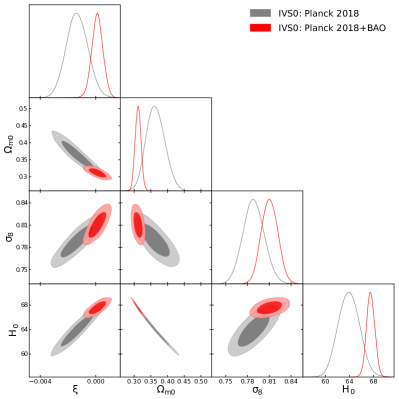
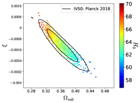
We show the observational constraints on this interacting cosmic scenario in Table 3 and in Fig. 1 for Planck 2018 alone and Planck 2018+BAO data. We include BAO with Planck 2018 in order to break the degeneracies between the parameters. From Planck 2018 data alone we find that is allowed at more than 68% CL (). So, a very mild interaction in the dark sector is signaled by Planck data alone, however, when BAO data are added to Planck CMB, becomes very small compared to its estimation from Planck CMB alone, but within 68% CL, is consistent (). The Hubble constant, assumes very lower value (, 95% CL, Planck 2018) compared to Planck’s CDM based estimation Aghanim:2018eyx but with high error bars as one can see. When BAO are added to Planck 2018, goes up with reduced error bars (, 95%, Planck 2018+BAO) and becomes consistent with Planck’s CDM based estimation Aghanim:2018eyx . So, as we can see that the tension on is not reconciled within this interacting scenario.
Regarding the estimation of , we find a very strong anti correlation with , and hence this parameter behaves accordingly with the increase or reduction of the Hubble constant. An interesting observation from Fig. 1, specifically from the joint contour is that, after the addition of BAO data to Planck 2018, the contour becomes vertical offering no correlation between them, while we note that for Planck 2018 data alone, the correlation between these two parameters are existing.
In summary, for this interaction model we find a very mild interaction in the dark sector which is much consistent with the non-interaction cosmology.
| Parameters | Planck 2018 | Planck 2018+BAO |
|---|---|---|
IV.2 IVS1
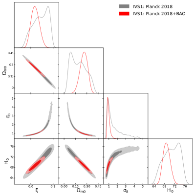
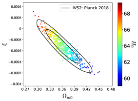
The summary of the observational constraints on this interaction model has been shown in Table 4 and in Fig. 2. One can clearly see that the estimations of the coupling parameter for both Planck 2018 and Planck 2018+BAO are large compared to the previous interacting scenario IVS0. For Planck 2018, we see that at more than 68% CL, (, 68% CL), but within 95% CL, is allowed. For Planck 2018+BAO, within 68% CL, is consistent. So, concerning the estimations of the coupling parameter, we can safely conclude that a mild interaction is allowed within this interaction scenario.
Concerning the estimation of , we find an interesting observation as follows. For Planck 2018, we find that takes a very high value with respect to the CDM based Planck’s estimation Aghanim:2018eyx having in addition significantly high error bars that enables us it to reach its local estimation ( Km at 68% CL) Riess:2019cxk , and thus, within 68% CL, the tension on is clearly alleviated. When BAO data are added to Planck 2018, the mean value of is lowered with reduced error bars where at 68% CL. So, compared to the minimal CDM cosmology, in this scenario the tension is less but not alleviated when we look at the measurement from Riess:2019cxk .
Thus, in summary, this interaction model has the ability to alleviate the tension offering a mild evidence of an interaction in the dark sector which is more pronounced for Planck 2018 alone.
| Parameters | Planck 2018 | Planck 2018+BAO |
|---|---|---|
IV.3 IVS2
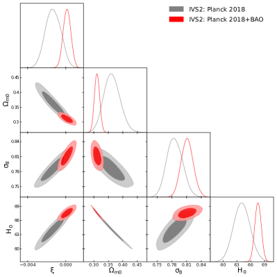
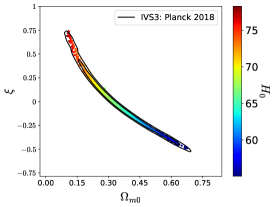
We show the observational constraints for this interacting scenario in Table 5 and in Fig. 3. In a similar fashion we concentrate on the key parameters and for this model. Note that the observational constraints for this model are almost similar to the IVS0 scenario. Thus, similar to IVS0 scenario, for this interaction model, an evidence of a non-null interaction at more than 68% CL is favored (, 68% CL, Planck 2018) for Planck 2018 data. While for Planck 2018+BAO, is consistent within 68% CL.
Concerning the estimations of for both Planck 2018 and Planck 2018+BAO, we find that for Planck 2018, it takes lower values with high error bars unlike to what we find in CDM based estimation Aghanim:2018eyx . Thus, the tension on remains true for Planck 2018 data. However, when BAO data are added to Planck 2018, slightly goes up with reduced error bars, but effectively the tension is not alleviated.
| Parameters | Planck 2018 | Planck 2018+BAO |
|---|---|---|
IV.4 IVS3
Finally, we consider the last interaction model in this series. Let us note that it is a nonlinear interaction model in the energy densities of the dark sectors’ components unlike the previous three interaction models which are linear in the energy densities of DM and DE. So, concerning its structure, it has certain interest in this context. In a similar way we summarize the observational constraints for this model in Table 6 and in Fig. 4.
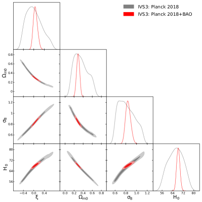
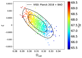
Concerning the observational constraints on the coupling parameter , we notice that for both Planck 2018 and Planck 2018+BAO, is consistent within 68% CL. For Planck 2018 alone: (68% CL) and for Planck 2018+BAO: (68% CL). However, both the datasets allow the nonzero values of the coupling parameter. So, the possibility of an interaction in the dark sector through this coupling function is equally probable.
From the constraints of , we see that Planck 2018 alone estimates a lower with very high error bars (, 68% CL), and due to this, as one can see, within 68% CL, it almost reaches the local estimation of Riess:2019cxk , and thus, the tension on is alleviated. Note that the alleviation of the tension is purely due to the error bars. However, when BAO data are added to Planck 2018, goes up but its error bars are reduced significantly compared to the error bars for Planck 2018, and eventually, the tension is not solved. We can say that the tension on is slightly weakened.
Therefore, in conclusion, within this interaction model, a mild coupling between DM and DE is supported by the observational data. Additionally, the model is also able to alleviate the tension due to its large error bars.
| Parameters | Planck 2018 | Planck 2018+BAO |
|---|---|---|
IV.5 Model comparisons
In the previous subsections we have described the observational constraints on the prescribed IVS scenarios. In this section we aim to compare the models through their observational direction as well as we also perform a Bayesian evidence analysis in order to test the observational viability of the models with respect to some reference model. Since CDM is the ideal choice to compare the interacting cosmological models under consideration, therefore, for Bayesian evidence analysis, we set CDM as the base/reference model.
In the first half of this section we compare the models focusing on their observational constraints as well as their effects on the large scale of the universe. In the second half of this subsection we provide the Bayesian evidence analysis for all the models with respect to the base CDM model.
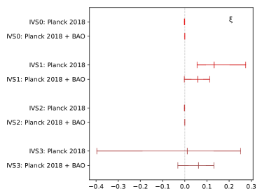
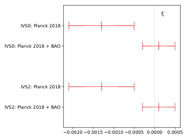
In Fig. 5, we show the whisker graphs for the coupling parameter of all the interacting scenarios, namely, IVS0, IVS1, IVS2 and IVS3, considering the analyses Planck 2018 and Planck 2018+BAO. Let us note that for IVS0 and IVS2, the region of coincides with the vertical line representing . The reason for such an overlap is that, for both IVS0 and IVS2, the constraints on are very close to zero (see Tables 3 and 5 for this purpose). That is why in the right graph of Fig. 5 we have separately shown the whisker plot for IVS0 and IVS2. Now, from the left graph, one can safely conclude that models IVS1 and IVS3 assume similar constraints, although for IVS3, is allowed. While the constraints from IVS0 and IVS2 are almost same. This is pretty clear from the right graph of Fig. 5.
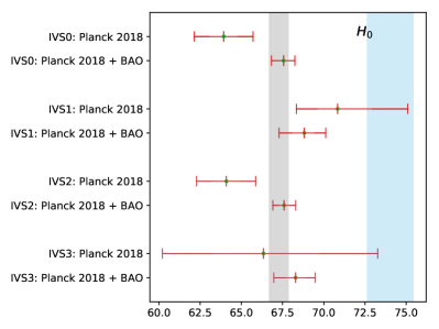
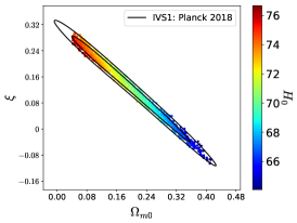
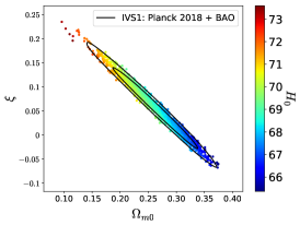
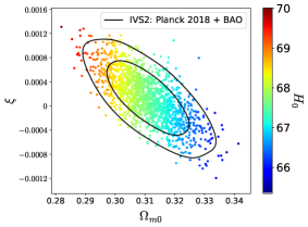
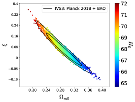
In order to understand how the present IVS models could be effective in alleviating/solving the tension, in Fig. 6, we show the whisker graph for (at 68% CL) for Planck 2018 and Planck 2018+BAO. The grey vertical band corresponds to estimated by the Planck 2018 release Aghanim:2018eyx and the pale blue vertical band denotes the estimation by SH0ES collaboration Riess:2019cxk . Let us first consider the response of all interacting scenarios to the tension for Planck 2018 data only. Looking at the estimated values of from different interacting scenarios, namely, Km s-1 Mpc-1 at 68% CL (for IVS0); Km s-1 Mpc-1 at 68% CL (for IVS1); Km s-1 at 68% CL (for IVS2); and Km s-1 Mpc-1 at 68% CL (for IVS3), one can clearly see that for IVS1, the mean value of is very high compared to other interacting scenarios in this work and the minimal CDM cosmology by Planck (where Km s-1 Mpc-1 at 68% CL for Planck TT,TE,EE+lowE Aghanim:2018eyx ). Now, due to the large error bars on for IVS1, the tension on is much alleviated. This is pretty clear from the whisker graph shown in Fig. 6. However, for IVS3, although has very high error bars ( Km s-1 Mpc-1 at 68% CL), but due to very small mean value ( Km s-1 Mpc-1), one cannot strongly argue that the tension on is satisfactorily alleviated. One can actually say that the tension on in this case is very mildly weakened just because of such high error bars on . When BAO data are added to Planck 2018, the combined dataset Planck 2018+BAO, as one can clearly see from the whisker graph in Fig. 6, cannot alleviate the tension on for IVS0 and IVS2. However, for IVS1 and IVS3, one can say that the tension on is very mildly weakened (see Fig. 6) due to slightly higher mean values of together with its higher error bars (see the Planck 2018+BAO columns in Tables 4 and 6) compared to the Planck’s estimation within the minimal CDM cosmology Aghanim:2018eyx . Finally, one might be interested to look at the 3D scattered plots for the IVS models shown in Fig. 7 and 8. From the scattered plots displayed in Fig. 7 and 8 one can understand the behaviour of the coupling parameter, , with higher and lower values of the Hubble constant, . For both Planck 2018 and Planck 2018+BAO, as we can see, for higher values of , assumes (although mildly) positive values, indicating an energy transfer from pressureless DM to DE. For lower values of , exactly opposite scenario is confirmed. The scattered plots actually give a nice statistical comparisons between the models.
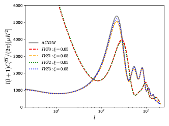
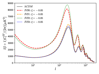
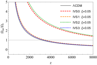
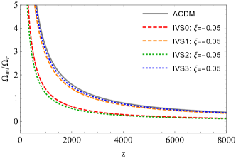
We also display in Fig. 9 the temperature anisotropy in the CMB TT spectra for all the IVS models using some specific values of the dimensionless coupling parameter . In the upper panel of Fig. 9 we show the CMB TT spectra for a specific positive value of and in the lower plot of Fig. 9 we display the same physical quantity for negative value of the coupling parameter, that means, . For comparison purpose, we have also included the non-interacting CDM scenario (). One can quickly realize that IVS0 and IVS2 are quite different compared to IVS1 and IVS3. Let us describe the physics behind the plots. From the upper plot of Fig. 9, one can see that for all IVS models, the heights of the first acoustic peak in the CMB TT spectrum, are less than the height of the first acoustic peak for the non-interacting CDM model. One can understand this phenomena from the evolution of the matter-radiation equality for all the IVS models. It is clear that if we add an interaction in the dark sector, the evolution of the CDM sector will not follow its usual evolution which is , hence, the evolution of the matter sector, that includes CDM and baryons, will definitely change from its usual evolution, and hence the matter-radiation equality will alter. If one looks at the upper plot of Fig. 10, it is clear that for all IVS models, the matter-radiation equality happens earlier for compared to the non-interacting CDM model. Due to earlier matter-radiation equality, the sound horizon is decreased, hence, for the present IVS models, the first peak in the CMB TT spectrum is decreased. For IVS0 and IVS2, the matter-radiation equality happens much earlier compared to IVS1 and IVS3, and this has been encoded in the CMB TT spectrum in terms of significant reduction of the first peak compared to other two IVS models. On the other hand, for , exactly the opposite scenario happens in the CMB TT spectrum (see the lower panel of Fig. 9) and this behaviour become clear when one looks at the corresponding matter-radiation equality presented in the lower plot of Fig. 10.
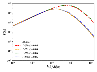
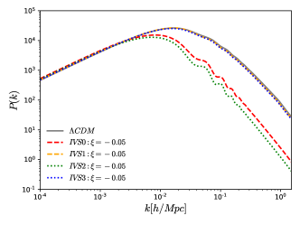
We also investigate the effects of the IVS models in the matter power spectrum. In Fig. 11 we show the matter power spectrum for all the IVS models for two specific values of the coupling parameter, namely, (upper panel of Fig. 11) and (lower panel of Fig. 11). We again find that the behaviour of IVS0 and IVS2 are completely different (in fact, violent) compared to the other IVS models. To understand the behaviour of various IVS models compared to the no-interaction scenario, we have considered the matter power spectrum for the non-interacting CDM model. From the upper plot of Fig. 11 we see that the amplitude of the matter power spectrum for all IVS models increases compared to the case. The significant increase in the matter power spectrum is transparent for IVS0 and IVS2 while for other two IVS models, it is quite difficult to understand the changes in the matter power spectrum from the non-interacting scenario (). The enhancement in the matter power spectrum is for the earlier matter-radiation equality, see the upper plot of Fig. 10. The reverse situation occurs for (see the lower plot of Fig. 11). In this case the matter power spectrum are suppressed and this again corresponds to the late matter-radiation equality as shown in the lower plot of Fig. 10.
Thus, from the behaviour of the IVS models presented in the CMB TT and matter power spectra shown respectively in Fig. 9 and 11, it is clearly pronounced that models IVS0 and IVS2 are significantly different from the rest two IVS models, namely, IVS1 and IVS3, and additionally, they are very far from the non-interacting CDM model which is only detected through the analysis of formation of structure of the universe.
Finally, we perform the Bayesian evidence analysis for a better understanding on the models with respect to some reference model. To calculate the evidences we use the MCEvidence Heavens:2017afc ; Heavens:2017hkr , a cosmological code for computating the evidences of the interacting scenarios (also see Pan:2017zoh ; Yang:2018qmz for detailed descriptions). To quantify the observational support of the models, we use the revised Jeffrey’s scale through different values of . The strength of evidence of the underlying model () with respect to the reference CDM scenario () is characterized as follows Kass:1995loi : (i) for , a weak evidence, (ii) for , a Definite/Positive evidence; (iii) for , a strong evidence, and (iv) for , a very strong evidence for the reference CDM model (“”) against the underlying model (here the interacting scenario) is considered. In Table 7 we have summarized the values of . From Table 7 we find that CDM is favored by the observational data over all the IVS models, but the models, namely, IVS1 and IVS3 are relatively close to CDM compared to the remaining two IVS models (IVS0 and IVS2). So, in summary, the models IVS1 and IVS3 have some importance in the literature in light of the Bayesian evidence analysis.
| Dataset | Model | ||
|---|---|---|---|
| Planck 2018 | IVS0 | ||
| Planck 2018+BAO | IVS0 | ||
| Planck 2018 | IVS1 | ||
| Planck 2018+BAO | IVS1 | ||
| Planck 2018 | IVS2 | ||
| Planck 2018+BAO | IVS2 | ||
| Planck 2018 | IVS3 | ||
| Planck 2018+BAO | IVS3 |
V Concluding remarks
Interacting DM – DE models have gained potential interest for explaining various cosmological puzzles beginning from the cosmic coincidence problem to the tension. It has been almost 20 years as of now, interacting models have been investigated by various investigators. The interacting models are entirely dependent on the interaction function, , that determines the rate of energy transfer between the dark sectors DM and DE. Despite of a lot of investigations in this context, a fundamental question – what should be the possible functional form of – is still unknown to the cosmological community. Since the nature of DM and DE are unknown, it is very difficult to extract the exact functional form for the interaction function. Thus, the easiest approach followed from earlier to present time, is to assume some phenomenological functions for and then to test them using the available cosmological data. The lack of a definite mechanism to construct the interaction functions raises questions over the interaction models. This motivated us to investigate the interaction models from the field theoretical arguments with an aim to search for a valid route to find out the models that are widely used. Our answer is affirmative in this direction. We have shown that various linear and nonlinear interaction functions that have been widely examined in the past and present, can be derived. This is the main essence of this work and probably this is the first time in the literature where we show the exact derivations of some very well known interaction models having a solid field theoretic ground.
We then examine the interaction models using CMB data from Planck 2018 final release and with the BAO data. The inclusion of BAO to CMB is motivated to break the degeneracies in some parameters that may exist during the analysis with CMB data alone. The results are summarized in Tables 3, 4, 5 and 6. Our analyses show that although both Planck 2018 and Planck 2018+BAO mildly allow a non-zero interaction in the dark sector but seems to be the most consistent picture. We also find that the second interaction model, namely, IVS1 is the most promising candidate to alleviate the tension in an effective way. The models have been investigated further through their effects on the CMB TT and matter power spectrum. Such an analysis is really important because this offers more insights on the models. Our analyses clearly depict that IVS0 and IVS2 are different compared to other models. We found that presence of an interaction in the dark sector alters the matter-radiation equality and hence this effects are encoded in the CMB TT and matter power spectrum. We notice that IVS1 and IVS3 are relatively close to the CDM model.
Finally, we perform a qualitative comparisons between the IVS models through the observational constraints and the Bayesian evidence analysis with respect to the reference CDM scenario. We find that IVS0 and IVS2 behave similarly, on the other hand, IVS1 and IVS3 behave similarly, but the last two models have essential advantages when we make the Bayesian evidence analysis. However, it is true that the CDM scenario is still preferred over the IVS models.
VI Acknowledgments
The authors thank the referee for some useful comments that helped us to improve the quality of the manuscript. SP has been supported by the Mathematical Research Impact-Centric Support Scheme (MATRICS), File No. MTR/2018/000940, given by the Science and Engineering Research Board (SERB), Govt. of India. WY was supported by the National Natural Science Foundation of China under Grants No. 11705079 and No. 11647153.
References
- (1) Y. L. Bolotin, A. Kostenko, O. A. Lemets and D. A. Yerokhin, Cosmological Evolution With Interaction Between Dark Energy And Dark Matter, Int. J. Mod. Phys. D 24, no. 03, 1530007 (2015) [arXiv:1310.0085 [astro-ph.CO]].
- (2) B. Wang, E. Abdalla, F. Atrio-Barandela and D. Pavón, Dark Matter and Dark Energy Interactions: Theoretical Challenges, Cosmological Implications and Observational Signatures, Rept. Prog. Phys. 79, no. 9, 096901 (2016) [arXiv:1603.08299 [astro-ph.CO]].
- (3) L. Amendola, Coupled quintessence, Phys. Rev. D 62, 043511 (2000), [astro-ph/9908023].
- (4) D. Tocchini-Valentini and L. Amendola, Stationary dark energy with a baryon dominated era: Solving the coincidence problem with a linear coupling, Phys. Rev. D 65, 063508 (2002) [astro-ph/0108143].
- (5) L. Amendola and C. Quercellini, Tracking and coupled dark energy as seen by WMAP, Phys. Rev. D 68, 023514 (2003) [astro-ph/0303228].
- (6) S. del Campo, R. Herrera and D. Pavón, Toward a solution of the coincidence problem, Phys. Rev. D 78, 021302 (2008) [arXiv:0806.2116 [astro-ph]].
- (7) S. del Campo, R. Herrera and D. Pavón, Interacting models may be key to solve the cosmic coincidence problem, J. Cosmol. Astropart. Phys. 0901, 020 (2009) [arXiv:0812.2210 [gr-qc]].
- (8) C. Wetterich, The cosmon model for an asymptotically vanishing time-dependent cosmological constant, Astron. Astrophys. 301, 321 (1995) [arXiv:hep-th/9408025].
- (9) R. G. Cai and A. Wang, Cosmology with interaction between phantom dark energy and dark matter and the coincidence problem, JCAP 0503, 002 (2005) [hep-th/0411025].
- (10) J. D. Barrow and T. Clifton, Cosmologies with energy exchange, Phys. Rev. D 73, 103520 (2006) [gr-qc/0604063].
- (11) J. H. He and B. Wang, Effects of the interaction between dark energy and dark matter on cosmological parameters, JCAP 0806, 010 (2008) [arXiv:0801.4233 [astro-ph]].
- (12) J. Väliviita, E. Majerotto and R. Maartens, Instability in interacting dark energy and dark matter fluids, JCAP 0807, 020 (2008) [arXiv:0804.0232 [astro-ph]].
- (13) E. Majerotto, J. Väliviita and R. Maartens, Adiabatic initial conditions for perturbations in interacting dark energy models, Mon. Not. Roy. Astron. Soc. 402, 2344 (2010) [arXiv:0907.4981 [astro-ph.CO]].
- (14) J. Väliviita, R. Maartens and E. Majerotto, Observational constraints on an interacting dark energy model, Mon. Not. Roy. Astron. Soc. 402, 2355 (2010) arXiv:0907.4987 [astro-ph.CO]
- (15) T. Clemson, K. Koyama, G. B. Zhao, R. Maartens and J. Väliviita, Interacting Dark Energy – constraints and degeneracies, Phys. Rev. D 85, 043007 (2012) [arXiv:1109.6234 [astro-ph.CO]].
- (16) R. C. Nunes and E. M. Barboza, Dark matter-dark energy interaction for a time-dependent EoS parameter, Gen. Rel. Grav. 46, 1820 (2014) [arXiv:1404.1620 [astro-ph.CO]].
- (17) V. Salvatelli, N. Said, M. Bruni, A. Melchiorri and D. Wands, Indications of a late-time interaction in the dark sector, Phys. Rev. Lett. 113, 181301 (2014) [arXiv:1406.7297 [astro-ph.CO]].
- (18) W. Yang and L. Xu, Cosmological constraints on interacting dark energy with redshift-space distortion after Planck data, Phys. Rev. D 89, 083517 (2014) [arXiv:1401.1286 [astro-ph.CO]].
- (19) W. Yang and L. Xu, Coupled dark energy with perturbed Hubble expansion rate, Phys. Rev. D 90, no. 8, 083532 (2014) [arXiv:1409.5533 [astro-ph.CO]].
- (20) S. Pan and S. Chakraborty, Will there be again a transition from acceleration to deceleration in course of the dark energy evolution of the universe?, Eur. Phys. J. C 73, 2575 (2013) [arXiv:1303.5602 [gr-qc]].
- (21) S. Pan and S. Chakraborty, A cosmographic analysis of holographic dark energy models, Int. J. Mod. Phys. D 23, no. 11, 1450092 (2014) [arXiv:1410.8281 [gr-qc]].
- (22) S. Pan, S. Bhattacharya and S. Chakraborty, An analytic model for interacting dark energy and its observational constraints, Mon. Not. Roy. Astron. Soc. 452, no. 3, 3038 (2015) [arXiv:1210.0396 [gr-qc]].
- (23) R. C. Nunes, S. Pan and E. N. Saridakis, New constraints on interacting dark energy from cosmic chronometers, Phys. Rev. D 94, 023508 (2016) [arXiv:1605.01712 [astro-ph.CO]].
- (24) S. Kumar and R. C. Nunes, Probing the interaction between dark matter and dark energy in the presence of massive neutrinos, Phys. Rev. D 94, 123511 (2016) [arXiv:1608.02454 [astro-ph.CO]].
- (25) W. Yang, H. Li, Y. Wu and J. Lu, Cosmological constraints on coupled dark energy, JCAP 1610, 007 (2016) [arXiv:1608.07039 [astro-ph.CO]].
- (26) C. van de Bruck, J. Mifsud and J. Morrice, Testing coupled dark energy models with their cosmological background evolution, Phys. Rev. D 95, 043513 (2017) [arXiv:1609.09855 [astro-ph.CO]].
- (27) S. Pan and G. S. Sharov, A model with interaction of dark components and recent observational data, Mon. Not. Roy. Astron. Soc. 472, 4736 (2017) [arXiv:1609.02287 [gr-qc]].
- (28) G. S. Sharov, S. Bhattacharya, S. Pan, R. C. Nunes and S. Chakraborty, A new interacting two fluid model and its consequences, Mon. Not. Roy. Astron. Soc. 466, no. 3, 3497 (2017) [arXiv:1701.00780 [gr-qc]].
- (29) W. Yang, N. Banerjee and S. Pan, Constraining a dark matter and dark energy interaction scenario with a dynamical equation of state, Phys. Rev. D 95, 123527 (2017) [arXiv:1705.09278 [astro-ph.CO]].
- (30) R. Y. Guo, Y. H. Li, J. F. Zhang and X. Zhang, Weighing neutrinos in the scenario of vacuum energy interacting with cold dark matter: application of the parameterized post-Friedmann approach, JCAP 1705, no. 05, 040 (2017) [arXiv:1702.04189 [astro-ph.CO]].
- (31) M. Shahalam, S. D. Pathak, S. Li, R. Myrzakulov and A. Wang, Dynamics of coupled phantom and tachyon fields, Eur. Phys. J. C 77, no. 10, 686 (2017) [arXiv:1702.04720 [gr-qc]].
- (32) W. Yang, S. Pan and D. F. Mota, Novel approach toward the large-scale stable interacting dark-energy models and their astronomical bounds, Phys. Rev. D 96, no. 12, 123508 (2017) [arXiv:1709.00006 [astro-ph.CO]].
- (33) W. Yang, S. Pan and J. D. Barrow, Large-scale Stability and Astronomical Constraints for Coupled Dark-Energy Models, Phys. Rev. D 97, no. 4, 043529 (2018) [arXiv:1706.04953 [astro-ph.CO]].
- (34) S. Pan, A. Mukherjee and N. Banerjee, Astronomical bounds on a cosmological model allowing a general interaction in the dark sector, Mon. Not. Roy. Astron. Soc. 477, 1189 (2018) [arXiv:1710.03725 [astro-ph.CO]].
- (35) H. L. Li, J. F. Zhang, L. Feng and X. Zhang, Reexploration of interacting holographic dark energy model: Cases of interaction term excluding the Hubble parameter, Eur. Phys. J. C 77, no. 12, 907 (2017) [arXiv:1711.06159 [astro-ph.CO]].
- (36) L. Amendola, J. Rubio and C. Wetterich, Primordial black holes from fifth forces, Phys. Rev. D 97, no. 8, 081302 (2018) [arXiv:1711.09915 [astro-ph.CO]].
- (37) D. Bégué, C. Stahl and S. S. Xue, A model of interacting dark fluids tested with supernovae and Baryon Acoustic Oscillations data, Nucl. Phys. B 940, 312 (2019) [arXiv:1702.03185 [astro-ph.CO]].
- (38) W. Yang, S. Pan and A. Paliathanasis, Cosmological constraints on an exponential interaction in the dark sector, Mon. Not. Roy. Astron. Soc. 482, no. 1, 1007 (2019) [arXiv:1804.08558 [gr-qc]].
- (39) W. Yang, S. Pan, L. Xu and D. F. Mota, Effects of Anisotropic Stress in Interacting Dark Matter - Dark Energy Scenarios, Mon. Not. Roy. Astron. Soc. 482, no. 2, 1858 (2019) [arXiv:1804.08455 [astro-ph.CO]].
- (40) W. Yang, S. Pan, R. Herrera and S. Chakraborty, Large-scale (in) stability analysis of an exactly solved coupled dark-energy model, Phys. Rev. D 98, no. 4, 043517 (2018) [arXiv:1808.01669 [gr-qc]].
- (41) H. L. Li, L. Feng, J. F. Zhang and X. Zhang, Models of vacuum energy interacting with cold dark matter: Constraints and comparison, Sci. China Phys. Mech. Astron. 62, no. 12, 120411 (2019) [arXiv:1812.00319 [astro-ph.CO]].
- (42) R. von Marttens, L. Casarini, D. F. Mota and W. Zimdahl, Cosmological constraints on parametrized interacting dark energy, Phys. Dark Univ. 23, 100248 (2019) [arXiv:1807.11380 [astro-ph.CO]].
- (43) W. Yang, N. Banerjee, A. Paliathanasis and S. Pan, Reconstructing the dark matter and dark energy interaction scenarios from observations, Phys. Dark. Univ 26, 100383 (2019) [arXiv:1812.06854 [astro-ph.CO]].
- (44) M. Martinelli, N. B. Hogg, S. Peirone, M. Bruni and D. Wands, Constraints on the interacting vacuum–geodesic CDM scenario, Mon. Not. Roy. Astron. Soc. 488, no. 3, 3423 (2019) [arXiv:1902.10694 [astro-ph.CO]].
- (45) M. Asghari, J. Beltrán Jiménez, S. Khosravi and D. F. Mota, On structure formation from a small-scales-interacting dark sector, JCAP 1904, 042 (2019) [arXiv:1902.05532 [astro-ph.CO]].
- (46) A. Paliathanasis, S. Pan and W. Yang, Dynamics of nonlinear interacting dark energy models, Int. J. Mod. Phys. D 28, no. 12, 1950161 (2019) [arXiv:1903.02370 [gr-qc]].
- (47) S. Pan, W. Yang, C. Singha and E. N. Saridakis, Observational constraints on sign-changeable interaction models and alleviation of the tension, Phys. Rev. D 100, no. 8, 083539 (2019) [arXiv:1903.10969 [astro-ph.CO]].
- (48) W. Yang, S. Pan, E. Di Valentino, B. Wang and A. Wang, Forecasting Interacting Vacuum-Energy Models using Gravitational Waves, [arXiv:1904.11980 [astro-ph.CO]].
- (49) N. Zhang, Y. B. Wu, J. N. Chi, Z. Yu and D. F. Xu, Diagnosing the interacting Tsallis Holographic Dark Energy models, [arXiv:1905.04299 [gr-qc]].
- (50) W. Yang, S. Vagnozzi, E. Di Valentino, R. C. Nunes, S. Pan and D. F. Mota, Listening to the sound of dark sector interactions with gravitational wave standard sirens, JCAP 1907, 037 (2019) [arXiv:1905.08286 [astro-ph.CO]].
- (51) W. Yang, O. Mena, S. Pan and E. Di Valentino, Dark sectors with dynamical coupling, Phys. Rev. D 100, no. 8, 083509 (2019) arXiv:1906.11697 [astro-ph.CO].
- (52) S. Savastano, L. Amendola, J. Rubio and C. Wetterich, Primordial dark matter halos from fifth forces, Phys. Rev. D 100, no. 8, 083518 (2019) [arXiv:1906.05300 [astro-ph.CO]].
- (53) S. Pan, W. Yang, E. Di Valentino, E. N. Saridakis and S. Chakraborty, Interacting scenarios with dynamical dark energy: observational constraints and alleviation of the tension, Phys. Rev. D 100, no. 10, 103520 (2019) arXiv:1907.07540 [astro-ph.CO].
- (54) E. Di Valentino, A. Melchiorri, O. Mena and S. Vagnozzi, Non-minimal dark sector physics and cosmological tensions, arXiv:1910.09853 [astro-ph.CO].
- (55) W. Yang, S. Pan, R. C. Nunes and D. F. Mota, Dark calling Dark: Interaction in the dark sector in presence of neutrino properties after Planck CMB final release, arXiv:1910.08821 [astro-ph.CO].
- (56) R. von Marttens, L. Lombriser, M. Kunz, V. Marra, L. Casarini and J. Alcaniz, Dark degeneracy I: Dynamical or interacting dark energy?, arXiv:1911.02618 [astro-ph.CO].
- (57) G. Papagiannopoulos, P. Tsiapi, S. Basilakos and A. Paliathanasis, Dynamics and cosmological evolution in -varying cosmology, arXiv:1911.12431 [gr-qc].
- (58) S. Kumar and R. C. Nunes, Echo of interactions in the dark sector, Phys. Rev. D 96, no. 10, 103511 (2017) [arXiv:1702.02143 [astro-ph.CO]].
- (59) E. Di Valentino, A. Melchiorri and O. Mena, Can interacting dark energy solve the tension?, Phys. Rev. D 96, 043503 (2017) [arXiv:1704.08342 [astro-ph.CO]].
- (60) W. Yang, S. Pan, E. Di Valentino, R. C. Nunes, S. Vagnozzi and D. F. Mota, Tale of stable interacting dark energy, observational signatures, and the tension, JCAP 1809, no. 09, 019 (2018) [arXiv:1805.08252 [astro-ph.CO]].
- (61) W. Yang, A. Mukherjee, E. Di Valentino and S. Pan, Interacting dark energy with time varying equation of state and the tension, Phys. Rev. D 98, no. 12, 123527 (2018) [arXiv:1809.06883 [astro-ph.CO]].
- (62) S. Kumar, R. C. Nunes and S. K. Yadav, Dark sector interaction: a remedy of the tensions between CMB and LSS data, Eur. Phys. J. C 79, no. 7, 576 (2019) [arXiv:1903.04865 [astro-ph.CO]].
- (63) E. Di Valentino, A. Melchiorri, O. Mena and S. Vagnozzi, Interacting dark energy after the latest Planck, DES, and measurements: an excellent solution to the and cosmic shear tensions, arXiv:1908.04281 [astro-ph.CO].
- (64) C. Van De Bruck and J. Mifsud, Searching for dark matter-dark energy interactions: going beyond the conformal case, Phys. Rev. D 97, no. 2, 023506 (2018) [arXiv:1709.04882 [astro-ph.CO]].
- (65) B. J. Barros, L. Amendola, T. Barreiro and N. J. Nunes, Coupled quintessence with a CDM background: removing the tension, JCAP 1901, no. 01, 007 (2019) [arXiv:1802.09216 [astro-ph.CO]].
- (66) S. M. Carroll, Quintessence and the rest of the world, Phys. Rev. Lett. 81, 3067 (1998) [astro-ph/9806099].
- (67) A. P. Billyard and A. A. Coley, Interactions in scalar field cosmology, Phys. Rev. D 61, 083503 (2000) [arXiv:astro-ph/9908224].
- (68) A. Nunes, J. P. Mimoso and T. C. Charters, Scaling solutions from interacting fluids, Phys. Rev. D 63, 083506 (2001) [gr-qc/0011073].
- (69) E. J. Copeland, M. Sami and S. Tsujikawa, Dynamics of dark energy, Int. J. Mod. Phys. D 15, 1753 (2006) [hep-th/0603057].
- (70) K. Bamba, S. Capozziello, S. Nojiri and S. D. Odintsov, Dark energy cosmology: the equivalent description via different theoretical models and cosmography tests, Astrophys. Space Sci. 342, 155 (2012) [arXiv:1205.3421 [gr-qc]].
- (71) E. Elizalde, S. Nojiri and S. D. Odintsov, Late-time cosmology in (phantom) scalar-tensor theory: Dark energy and the cosmic speed-up, Phys. Rev. D 70, 043539 (2004) [hep-th/0405034].
- (72) S. Nojiri, S. D. Odintsov and S. Tsujikawa, Properties of singularities in (phantom) dark energy universe, Phys. Rev. D 71, 063004 (2005) [hep-th/0501025].
- (73) S. Nojiri and S. D. Odintsov, Unifying phantom inflation with late-time acceleration: Scalar phantom-non-phantom transition model and generalized holographic dark energy, Gen. Rel. Grav. 38, 1285 (2006) [hep-th/0506212].
- (74) S. Capozziello, S. Nojiri and S. D. Odintsov, Unified phantom cosmology: Inflation, dark energy and dark matter under the same standard, Phys. Lett. B 632, 597 (2006) [hep-th/0507182].
- (75) B. Feng, X. L. Wang and X. M. Zhang, Dark energy constraints from the cosmic age and supernova, Phys. Lett. B 607, 35 (2005) [astro-ph/0404224].
- (76) P. A. R. Ade et al. [Planck Collaboration], Planck 2015 results. XIII. Cosmological parameters, Astron. Astrophys. 594, A13 (2016) [arXiv:1502.01589 [astro-ph.CO]].
- (77) N. Aghanim et al. [Planck Collaboration], Planck 2018 results. VI. Cosmological parameters, [arXiv:1807.06209 [astro-ph.CO]].
- (78) A. H. Chamseddine and V. Mukhanov, Mimetic dark matter, JHEP 1311, 135 (2013) [arXiv:1308.5410 [astro-ph.CO]].
- (79) A. H. Chamseddine, V. Mukhanov and A. Vikman, Cosmology with Mimetic Matter, JCAP 1406, 017 (2014) [arXiv:1403.3961 [astro-ph.CO]].
- (80) R. Myrzakulov, L. Sebastiani and S. Vagnozzi, Inflation in -theories and mimetic gravity scenario, Eur. Phys. J. C 75, 444 (2015) [arXiv:1504.07984 [gr-qc]].
- (81) G. Cognola, R. Myrzakulov, L. Sebastiani, S. Vagnozzi and S. Zerbini, Covariant Hor̆ava-like and mimetic Horndeski gravity: cosmological solutions and perturbations, Class. Quant. Grav. 33, no. 22, 225014 (2016) [arXiv:1601.00102 [gr-qc]].
- (82) L. Sebastiani, S. Vagnozzi and R. Myrzakulov, Mimetic gravity: a review of recent developments and applications to cosmology and astrophysics, Adv. High Energy Phys. 2017, 3156915 (2017) [arXiv:1612.08661 [gr-qc]].
- (83) S. Vagnozzi, Recovering a MOND-like acceleration law in mimetic gravity, Class. Quant. Grav. 34, no. 18, 185006 (2017) [arXiv:1708.00603 [gr-qc]].
- (84) J. de Haro, L. Aresté Saló and S. Pan, Limiting curvature mimetic gravity and its relation to Loop Quantum Cosmology, Gen. Rel. Grav. 51, no. 4, 49 (2019) [arXiv:1803.09653 [gr-qc]].
- (85) V. F. Mukhanov, H. A. Feldman and R. H. Brandenberger, Theory of cosmological perturbations, Phys. Rept. 215, 203 (1992).
- (86) C. P. Ma and E. Bertschinger, Cosmological perturbation theory in the synchronous and conformal Newtonian gauges, Astrophys. J. 455, 7 (1995) arXiv:astro-ph/9506072.
- (87) K. A. Malik and D. Wands, Cosmological perturbations, Phys. Rept. 475, 1 (2009) [arXiv:0809.4944 [astro-ph]].
- (88) Y. Wang, D. Wands, G. B. Zhao and L. Xu, Post- constraints on interacting vacuum energy, Phys. Rev. D 90 (2014) no.2, 023502 [arXiv:1404.5706 [astro-ph.CO]].
- (89) P. S. Corasaniti, Slow-Roll Suppression of Adiabatic Instabilities in Coupled Scalar Field-Dark Matter Models, Phys. Rev. D 78, 083538 (2008) [arXiv:0808.1646 [astro-ph]].
- (90) N. Aghanim et al. [Planck Collaboration], Planck 2018 results. VIII. Gravitational lensing, arXiv:1807.06210 [astro-ph.CO].
- (91) N. Aghanim et al. [Planck Collaboration], Planck 2018 results. V. CMB power spectra and likelihoods, arXiv:1907.12875 [astro-ph.CO].
- (92) F. Beutler et al., The 6dF Galaxy Survey: Baryon Acoustic Oscillations and the Local Hubble Constant, Mon. Not. Roy. Astron. Soc. 416, 3017 (2011) [arXiv:1106.3366 [astro-ph.CO]].
- (93) A. J. Ross, L. Samushia, C. Howlett, W. J. Percival, A. Burden and M. Manera, The clustering of the SDSS DR7 main Galaxy sample I. A 4 per cent distance measure at , Mon. Not. Roy. Astron. Soc. 449, 835 (2015) [arXiv:1409.3242 [astro-ph.CO]].
- (94) H. Gil-Marín et al., The clustering of galaxies in the SDSS-III Baryon Oscillation Spectroscopic Survey: BAO measurement from the LOS-dependent power spectrum of DR12 BOSS galaxies, Mon. Not. Roy. Astron. Soc. 460, 4210 (2016) [arXiv:1509.06373 [astro-ph.CO]].
- (95) A. Lewis and S. Bridle, Cosmological parameters from CMB and other data: A Monte Carlo approach, Phys. Rev. D 66, 103511 (2002) [astro-ph/0205436].
- (96) A. Lewis, A. Challinor and A. Lasenby, Efficient computation of CMB anisotropies in closed FRW models, Astrophys. J. 538, 473 (2000) [astro-ph/9911177].
- (97) A. Gelman and D. Rubin, Inference from iterative simulation using multiple sequences, Statistical Science 7, 457 (1992).
- (98) A. G. Riess, S. Casertano, W. Yuan, L. M. Macri and D. Scolnic, Large Magellanic Cloud Cepheid Standards Provide a 1% Foundation for the Determination of the Hubble Constant and Stronger Evidence for Physics beyond CDM, Astrophys. J. 876, no. 1, 85 (2019) [arXiv:1903.07603 [astro-ph.CO]].
- (99) A. Heavens, Y. Fantaye, A. Mootoovaloo, H. Eggers, Z. Hosenie, S. Kroon and E. Sellentin, Marginal Likelihoods from Monte Carlo Markov Chains, arXiv:1704.03472 [stat.CO].
- (100) A. Heavens, Y. Fantaye, E. Sellentin, H. Eggers, Z. Hosenie, S. Kroon and A. Mootoovaloo, No evidence for extensions to the standard cosmological model, Phys. Rev. Lett. 119, no. 10, 101301 (2017). [arXiv:1704.03467 [astro-ph.CO]].
- (101) S. Pan, E. N. Saridakis and W. Yang, Observational Constraints on Oscillating Dark-Energy Parametrizations, Phys. Rev. D 98, no. 6, 063510 (2018) [arXiv:1712.05746 [astro-ph.CO]].
- (102) W. Yang, S. Pan, E. Di Valentino, E. N. Saridakis and S. Chakraborty, Observational constraints on one-parameter dynamical dark-energy parametrizations and the tension, Phys. Rev. D 99, no. 4, 043543 (2019) [arXiv:1810.05141 [astro-ph.CO]].
- (103) R. E. Kass and A. E. Raftery, Bayes factors, J. Am. Statist. Assoc. 90, no.430, 773 (1995).