STAViS: Spatio-Temporal AudioVisual Saliency Network

Abstract

We introduce STAViS, a spatio-temporal audiovisual saliency network that combines spatio-temporal visual and auditory information in order to efficiently address the problem of saliency estimation in videos. Our approach employs a single network that combines visual saliency and auditory features and learns to appropriately localize sound sources and to fuse the two saliencies in order to obtain a final saliency map. The network has been designed, trained end-to-end, and evaluated on six different databases that contain audiovisual eye-tracking data of a large variety of videos. We compare our method against 8 different state-of-the-art visual saliency models. Evaluation results across databases indicate that our STAViS model outperforms our visual only variant as well as the other state-of-the-art models in the majority of cases. Also, the consistently good performance it achieves for all databases indicates that it is appropriate for estimating saliency “in-the-wild”. The code is available at https://github.com/atsiami/STAViS.

1 Introduction

Audio is present in the majority of scenes where vision is also present. Nature as well as everyday life offer unlimited examples of multi-sensory and cross-modal events, a large amount of which concern auditory and visual senses. Audiovisual integration is a well studied phenomenon in neuroscience with interesting findings that have motivated research in the area [36, 37, 60]. Many of them provide sufficient evidence that human attention and perception is influenced by audiovisual stimuli in a different way than auditory or visual stimuli in isolation. For example, the well-known McGurk effect [35] proved that attention can be heavily affected by incongruent audiovisual stimuli, leading to illusionary perceptions. On the other hand, congruent ones, like in the pip & pop effect [59], can lead to enhanced attention. Modeling human attention is important in a variety of applications, like video summarization [28, 16], robotics [15, 30, 67], and virtual reality [54].

Despite the previously mentioned evidence of a strong audiovisual interplay, audio modality has been rather neglected when modeling human attention, with most computer vision research focusing only on visual information. We aim to address the problem of saliency estimation in videos “in-the-wild”, namely how bottom-up human attention is modeled, by integrating auditory information into visual saliency, without prior knowledge of the video content. Fig. 1 highlights and motivates the problem we aim to address: tolling bells is an audiovisual event. The depicted frames, with their eye-tracking data superimposed, exhibit an example of human attention in an audiovisual scene. This attention can be much better captured by an audiovisual attention model than by a visual-only one, as the corresponding saliency maps indicate.

Figure 1: Example frames with their eye-tracking data of a bell tolling. The second row depicts the saliency maps produced by our visual-only saliency network, while the third row is the output of our proposed STAViS network, which succeeds in better capturing human attention.

In parallel, Convolutional Neural Networks (CNNs) have infiltrated computer vision and have enhanced dramatically the performance in the majority of spatial tasks in computer vision, such as object detection or semantic segmentation [53, 22, 21]. The huge amounts of video data that are becoming more and more available through online sources, enable and at the same time require continuously better performance in tasks like activity recognition, video saliency, scene analysis or video summarization, imposing the need to exploit not only spatial information, but also temporal [8, 48, 28]. Similar advances have also been achieved in audio processing areas, such as acoustic event detection [45], speech recognition [18, 10], sound localization [57], by using deep learning techniques.

As an additional free of charge source of information, auditory stream has been incorporated in many video-related applications during the last three years [1, 69]. Audio contains rich information that when integrated with spatio-temporal visual information, it facilitates learning and improves performance in many traditionally visual-only tasks. Most importantly, audio comes for free, as it is already included in the majority of videos and synchronized with the visual stream. We are particularly interested in audiovisual attention modeling, through audiovisual saliency, where the main goal is to predict human fixations in a video.

We propose STAViS, a novel spatio-temporal audiovisual saliency network that combines spatio-temporal visual with auditory information to efficiently address the problem of saliency estimation in videos. We mainly aspire to make the next logical step in video saliency prediction by introducing a new audiovisual framework rather than propose just a better visual model. To our best knowledge, our proposed system is the first deep learning saliency approach that employs both video and audio and addresses the fixation prediction problem, except for concurrent work [56] where two independent networks for the two modalities are employed and their outputs are simply concatenated as a late fusion scheme. Our approach employs a single multimodal network that combines visual and auditory information at multiple stages and learns to appropriately fuse the two modalitites, in order to obtain a final saliency map. We propose ways to perform sound source localization in the video and subsequently fuse spatio-temporal auditory saliency with spatio-temporal visual saliency, in order to obtain the final audiovisual saliency map.

For visual saliency our approach is extending a state-of-the-art spatio-temporal saliency network, called SUSiNet [28], part of a multi-task network that jointly addresses 3 different problems: saliency estimation, activity recognition and video summarization. Regarding audio, we obtain audio features using SoundNet [3], a state-of-the-art CNN for acoustic event classification. For sound localization, we aim to retrieve the potential correspondences between auditory and visual streams, in the sense of cross-modal semantic concepts. We explore 3 different ways of locating sounds in a video, obtaining an auditory saliency map. Subsequently, we investigate fusion schemes to integrate spatio-temporal and auditory saliencies and obtain a final saliency map. We explore three alternatives as well.

The network has been designed, trained end-to-end and evaluated on 6 different databases that contain audiovisual eye-tracking data. These databases contain a large variety of videos, ranging from home-made videos to documentaries, and from short, simple videos to Hollywood movies. Our method is compared to 8 different state-of-the-art visual saliency models in all 6 databases. Evaluation results across databases indicate that STAViS model outperforms both the visual variant network and the other methods in the majority of cases. Also, its consistently good performance for all databases, indicates that it is suitable for estimating saliency in videos “in-the-wild”.

Figure 2: STAViS architecture: the spatio-temporal audiovisual network is based on the ResNet architecture and has one spatio-temporal visual path, one auditory path and their fusion.

2 Related Work

There is a very broad literature regarding visual saliency, both for classical approaches and for deep learning ones. On the other hand, audiovisual approaches in saliency are limited. Below, we describe the most notable works in visual saliency with deep methods, audiovisual saliency, and other recent audiovisual approaches in similar problems.

Visual Saliency: The early CNN-based approaches for saliency were based on the adaptation of pretrained CNN models for visual recognition tasks [31, 61]. Later, in [44] both shallow and deep CNN were trained end-to-end for saliency prediction while [23, 24] trained the networks by optimizing common saliency evaluation metrics. In [43] the authors employed end-to-end Generative Adversarial Networks (GAN), while [63] has utilized multi-level saliency information from different layers through skip connections. Long Short-term Memory (LSTM) networks have also been used for tracking visual saliency both in static images [11] and video stimuli [64, 65, 34]. In order to improve saliency estimation in videos, many approaches employ multi-stream networks, such as RGB/Optical Flow (OF) [4, 32], RGB/OF/Depth [33], or multiple subnets such as objectness/motion [25] or saliency/gaze [17] pathways. Another recent approach [38] employs a 3D fully-convolutional network with temporal aggregation, based on the assumption that the saliency map of any frame can be predicted by considering a limited number of past frames.

Audiovisual saliency models: The first attempts in modeling audiovisual saliency were application-specific [49, 50, 46, 9, 47, 52], employing mostly traditional signal processing techniques both for visual saliency and audio localization. Coutrot and Guyader [13, 12, 14] and Song [55] have tried to more directly validate their models with humans. After estimating the visual saliency map they explicitly weigh the face image regions appropriately to generate an audiovisual saliency map to better account for eye fixations during movie viewing. Also, Min et al. [40, 39] developed an audiovisual attention model for predicting eye fixations in scenes containing moving, sound-generating objects. For auditory attention, they employed an auditory source localization method to localize the sound-generating object on the image and fuse it with visual saliency models. A more general model that is not application-specific that investigated ways to fuse audio and video for fixation prediction with signal processing techniques has been presented in [58].

Other deep audiovisual approaches: As mentioned before, during the last three years more and more attention is paid on integration of audio in traditionally visual-only problems, such as object localization or segmentation. In [1, 2] audiovisual correspondence in videos is learned without supervision resulting in good video and audio representations as well as in good classification in both modalities. Audiovisual representations learned in a self-supervised way and used for audiovisual scene analysis are also proposed in [51, 42], while in [57], the authors address the problem of audiovisual event localization in unconstrained videos. A system that learns to locate image regions that produce sound and creates a representation of the sound from each pixel is described in [69, 68]. Also, SoundNet [3] exploits the natural synchronization between vision and sound to learn an acoustic representation using two-million unlabeled videos, yielding improved performance in acoustic scene/object classification tasks. In [26], the authors exploit auditory and visual information to build effective models for both audio and video analysis from self-supervised temporal synchronization.

3 Spatio-Temporal AudioVisual Saliency Network

The proposed designed spatio-temporal audiovisual network for saliency estimation (Fig. 2) consists of a spatio-temporal visual module that computes visual saliency, an audio representation module that computes auditory features based on [3], a sound source localization module that computes spatio-temporal auditory saliency, an audiovisual saliency estimation module that combines and fuses the visual and auditory saliencies, and finally, the appropriate losses. These are described in detail in the next subsections.

3.1 Spatio-Temporal Visual Network

The architecture of our designed spatio-temporal network for visual saliency, depicted in Fig. 2, employs the general ResNet architecture [22] and specifically the 3D extension proposed initially for action classification [20]. The visual network pathway (dark purple color), with parameters $\mathbf{W}_{res}$, includes the first 4 ResNet convolutional blocks $\mathrm{conv1,conv2,conv3,conv4}$ that provide outputs $X^{1},X^{2},X^{3},X^{4}$, in different spatial and temporal scales. In parallel, an attention mechanism called Deeply Supervised Attention Module (DSAM) is applied by taking the element-wise product between each channel of the feature map $X^{m}$ and the attention map $M^{m}$, to enhance the most salient regions of these feature representations:

$$\tilde{X}^{m}=(1+M^{m})\odot X^{m},\quad m=1,\ldots,4.$$ (1)

The idea of deep supervision that is the core of DSAM has been used in edge detection [66], object segmentation [7] and static saliency [63], but contrary to these previous works, here DSAM’s role is double: It is used both for enhancing visual feature representations as well as for providing the multi-level saliency maps, as depicted by shades of green in Fig. 2. Thus, DSAM parameters $\mathbf{W}_{am}^{m}$ are trained both by the main-path of the visual network and the eye-tracking data through the skip connections of the Fig. 2.

Figure 3 shows the architecture of the DSAM module at level $m$. It includes an averaging pooling in the temporal dimension followed by two spatial convolution layers that provide the saliency features $S^{m}$ and the activation map $A^{m}$. Both representations are up-sampled (using the appropriate deconvolution layers) to the initial image dimensions and used for the deep supervision of the module as well as for the multi-level saliency estimation. A spatial softmax operation applied at the activation map $A^{m}(x,y)$ yields the attention map $M^{m}(x,y)$:

$$M^{m}(x,y)=\frac{\exp(A^{m}(x,y))}{\sum_{x}\sum_{y}\exp(A^{m}(x,y))}$$ (2)

3.2 Audio Representation Network

For the audio representation we select to work directly on the sound waveforms and employ an 1-D fully convolutional network, rather than compute time-frequency representations and apply 2D CNNs [26, 1, 69]. First, audio is cropped in order to match the visual frames duration (i.e. 16 frames). The employed network can handle variable length audio, thus no sub-sampling is required to address the sampling rate variation from video to video. Subsequently, a Hanning window is applied in order to weigh higher the central audio values representing the current time instance, but also include past and future values with attenuation [58]. Afterwards, for the high-level information encoding we employ a network architecture with parameters $\mathbf{W}_{a}$ based on the first seven layers of the SoundNet [3]. These layers are followed by a temporal max-pooling layer for obtaining a fixed dimension vector $f_{a}\in\mathbb{R}^{D_{a}}$ for the whole sequence.

Figure 3: Deeply Supervised Attention Module (DSAM) enhances the global network’s representations and provides the multi-level saliency maps for spatio-temporal saliency.

3.3 Sound Source Localization in Videos

The previous module’s goal is to produce good audio representations. Our next goal is to exploit these representations in order to detect cross-modal semantic concepts in videos. We essentially aim to retrieve correspondences between audio and spatio-temporal visual information, and thus obtain a spatio-temporal auditory saliency map. This can be viewed also as a spatial sound source localization problem. For example, a moving car, a speaking face or a rustling leaf are cross-modal events, where we need to detect where the audio comes from in the video.

Our approach selects as visual features the output of the 3D conv3 block $X^{3}$ (that has feature dimension $D_{v}$) as in this layer with have both rich semantic information for the visual stream and quite large resolution in the spatial domain. A temporal average pooling is applied in order to marginal out the temporal dimension and have a global representation $f_{v}\in\mathbb{R}^{D_{v}\times N_{X}\times N_{Y}}$ for the whole sequence. Since visual and auditory features have different feature dimensions, we re-project both in a hidden dimension $D_{h}$ by applying two different affine transformations:

$$\tilde{h}_{a}=\mathbf{U}_{a}\cdot f_{a}+\mathbf{b}_{a},\quad h_{v}=\mathbf{U}_{v}\cdot f_{v}+\mathbf{b}_{v},$$ (3)

where $\tilde{h}_{a}\in\mathbb{R}^{D_{h}}$, $h_{v}\in\mathbb{R}^{D_{h}\times N_{X}\times N_{Y}}$ and $\mathbf{U}_{a},\mathbf{b}_{a},\mathbf{U}_{v},\mathbf{b}_{v}$ are the corresponding learning parameters. We also apply a spatially tiling to the audio features to match the visual features spatial dimensions, getting $h_{a}\in\mathbb{R}^{D_{h}\times N_{X}\times N_{Y}}$.

For finding or learning correspondences between the audio and visual features $h_{a},h_{v}$ we have investigated three different approaches. In the first, we simply compute the cosine similarity between the two representation vectors which does not require any learning parameters and provides a single localization map $L_{1}\in\mathbb{R}^{N_{X}\times N_{Y}}$. Regarding the second approach, we take the weighted inner product of the vectors $h_{a},h_{v}$ at each pixel $(x,y)$, and we can get either a single or multiple localization maps $L_{2}^{j}\in\mathbb{R}^{N_{X}\times N_{Y}},\quad j=1,\dots,N_{out}$:

$$L_{2}^{j}(x,y)=\sum_{k=1}^{D_{h}}s^{j,k}\cdot h_{v}^{k}(x,y)\cdot h_{a}^{k}(x,y)+\beta^{j},$$ (4)

where $s^{j,k},\beta^{j}$ are learning parameters. In the third case, that constitutes also the proposed approach, a bilinear transformation is applied to the incoming multimodal data that can also yield either a single or multiple output maps $L_{3}^{j}\in\mathbb{R}^{N_{X}\times N_{Y}},\quad j=1,\dots,N_{out}$:

$$L_{3}^{j}(x,y)=h_{v}(x,y)^{T}\cdot\mathbf{M}^{j}\cdot h_{a}(x,y)+\mu^{j}$$

$$=\sum_{l=1}^{D_{h}}\sum_{k=1}^{D_{h}}M^{j,l,k}\cdot h_{v}^{l}(x,y)\cdot h_{a}^{k}(x,y)+\mu^{j},$$ (5)

where $M^{j,l,k},\mu^{j}$ are the learning parameters. Note that the previous approaches ($L_{1}$, $L_{2}$) are special cases of this bilinear one ($L_{3}$), that allows for richer interactions between the inputs. Specifically when the matrices $\mathbf{M}^{j}$ are diagonal, with $s^{j,k}$ as diagonal elements, we have the case of weighted inner product ($L_{2}$). When the matrix $\mathbf{M}$ is the unit matrix the result is very close (modulo a normalization factor) to the cosine similarity.

3.4 Audiovisual Saliency Estimation

We have now computed an auditory saliency map, expressed via source localization maps. However, there are many aspects in a video that can attract the human attention that may not be related to audio events. Thus, in order to build a multi-modal saliency estimation network that can perform well “in-the-wild” with any kind of stimuli, we need to also include the visual-only information as modeled by the spatio-temporal visual network. For that purpose an important contribution of this paper is the investigation of different ways to perform audiovisual fusion.

The simplest fusion scheme is to learn a linear weighted sum of the visual only map $S^{v}$ and an audio-related map $S^{a}$ (yielded by applying independent fully convolution layers to the multi-level concatenated visual saliency features $V^{j}~{}=~{}(S^{1}|\dots|S^{m}|\dots|S^{M})$ and the localization maps $L^{j}$ respectively): $S_{1}^{av}~{}=~{}w_{v}~{}\cdot~{}\sigma(S^{v})~{}+~{}w_{a}~{}\cdot~{}\sigma(S^{a})$, where $\sigma(\cdot)$ denotes the sigmoid activation function.

Moreover, inspired by previous signal processing based approaches for audiovisual saliency [58, 29], we also investigate an attention based scheme where the audio stream modulates the visual one: $S_{2}^{av}~{}=~{}\sigma(S^{v})~{}\odot~{}(1~{}+~{}\sigma(S^{a}))$. In case of multiple localization maps, we can multiply one by one the concatenated visual saliency features $V^{j}$ with the localization maps $L^{j}$ and then apply a fully convolution layer for taking the single saliency map: $\tilde{S}_{2}^{av,j}=\sigma(V^{j})\odot(1+\sigma(L^{j}))$.

However, as depicted in Fig. 2, our main and most general approach that allows more free interaction between the visual and audio-based features maps is to concatenate the multimodal features and then apply a convolution layer for their fusion in one saliency map: $S_{3}^{av}~{}=~{}\mathbf{W}_{cat}~{}*~{}(V|L)~{}+~{}\bm{\beta}_{av}$.

Finally, we can also apply a late fusion scheme of all the previous approaches expressed by a weighted learned sum: $S^{av}_{fus}=\tilde{w}_{v}\cdot\sigma(S^{v})+\tilde{w}_{a}\cdot\sigma(S^{a})+w_{av}\cdot\sigma(S^{3})$.

3.5 Saliency Losses

For the training of the parameters $\mathbf{W}_{v}$ that are associated with the visual stream, we construct a loss that compares the saliency map $S^{v}$ and the activations $A^{m}$ with the ground truth maps $Y_{sal}$ obtained by the eye-tracking data:

$$\begin{split}\mathcal{L}_{v}(\mathbf{W}_{v})=\mathcal{D}(\mathbf{W}_{v}|\sigma(S^{v}),Y_{sal})+\\ \sum_{m=1}^{4}\mathcal{D}(\mathbf{W}_{AM}^{m}|\sigma(A^{m}),Y_{sal}),\end{split}$$ (6)

where $\sigma(\cdot)$ denotes the sigmoid non-linearity and $\mathcal{D}(\cdot)$ is a loss function between the estimated and the ground truth 2D maps. When we train the parameters $\mathbf{W}_{av}$ of the audiovisual network, we use the trained visual-only network as a starting point and we do not use the skip connections of the DSAM modules:

$$\mathcal{L}_{av}(\mathbf{W}_{av})=\mathcal{D}(\mathbf{W}_{av}|\sigma(S^{av}),Y_{sal}).$$ (7)

Several different metrics to evaluate saliency are employed in order to compare the predicted saliency map $P\in[0,1]^{N_{X}\times N_{Y}}$ to the eye-tracking data [6]. As ground truth maps we can use either the map of fixation locations $Y_{fix}\in\{0,1\}^{N_{X}\times N_{Y}}$ on the image plane of size $N_{X}\times N_{Y}$ or the dense saliency map $Y_{den}\in[0,1]^{N_{X}\times N_{Y}}$ that is produced by convolving the binary fixation map with a gaussian kernel. Thus, as $\mathcal{D}(\cdot)$ we employ three loss functions associated with the different aspects of saliency evaluation. The first is the cross-entropy loss between the predicted map $P$ and the dense map $Y_{den}$:

$$\begin{split}\mathcal{D}_{CE}(\mathbf{W}|P,Y_{den})=-\sum_{x,y}Y_{den}(x,y)\odot\log(P(x,y;\mathbf{W}))\\ +(1-Y_{den}(x,y))\odot(1-\log(P(x,y;\mathbf{W}))).\end{split}$$ (8)

The second loss function is based on the linear Correlation Coefficient (CC) [6] that is widely used in saliency evaluation and measures the linear relationship between the predicted saliency $P$ and the dense ground truth map $Y_{den}$:

$$\mathcal{D}_{CC}(\mathbf{W}|P,Y_{den})=-\frac{\mathrm{cov}(P(x,y;\mathbf{W}),Y_{den}(x,y))}{\rho(P(x,y;\mathbf{W}))\cdot\rho(Y_{den}(x,y))},$$ (9)

where $\mathrm{cov},\rho$ denote the covariance and the standard deviation respectively. The last loss is derived from the Normalized Scanpath Saliency (NSS) metric [6], which is computed as the estimated map values $\tilde{P}(x,y;\mathbf{W})=\frac{P(x,y;\mathbf{W})-\mu(P(x,y;\mathbf{W}))}{\rho(P(x,y;\mathbf{W}))}$, after zero mean normalization and unit standardization, at human fixation locations ($Y_{fix}(x,y)=1$):

$$\mathcal{D}_{NSS}(\mathbf{W}|\tilde{P},Y_{fix})=-\frac{1}{N_{f}}\sum_{x,y}\tilde{P}(x,y;\mathbf{W})\odot Y_{fix}(x,y),$$ (10)

where $N_{f}=\sum_{x,y}Y_{fix}(x,y)$ denotes the total number of fixation points. The final loss of the $i$-th input sample is given by a weight combination of the losses $\mathcal{L}^{i}_{CE},\mathcal{L}^{i}_{CC},\mathcal{L}^{i}_{NSS}$ that are given either by Eq.(6) or Eq.(7) using the corresponding loss functions $\mathcal{D}^{i}_{CE},\mathcal{D}^{i}_{CC},\mathcal{D}^{i}_{NSS}$:

$$\mathcal{L}_{sal}^{i}(\mathbf{W})=w_{1}\mathcal{L}^{i}_{CE}+w_{2}\mathcal{L}^{i}_{CC}+w_{3}\mathcal{L}_{NSS}^{i},$$ (11)

where $w_{1},w_{2},w_{3}$ are the weights of each loss type.

3.6 Implementation

Our implementation and experimentation with the visual network uses as backbone the 3D ResNet-50 architecture [20] that has showed competitive performance against other deeper architectures for action recognition task, in terms of performance and computational budget. As starting point for $\mathbf{W}_{res}$ we used the weights from the pretrained model in the Kinetics 400 database. For the audio stream we employ the SoundNet (using 7 out of 8 layers) architecture [3] that is based on 1D temporal convolution and has been successfully applied in acoustic scene/event classification tasks. As starting point for our audio representation network parameters $\mathbf{W}_{a}$ we use the weights from the pretrained model that has been trained on two million videos from Flickr [3]. Training: For training we employ stochastic gradient descent with momentum 0.9, while we assign a weight decay of 1e-5 for regularization. We have also employed effective batchsizes of 128 samples, and multistep learning rate. First we train the visual-only spatio-temporal network and afterwards the whole audiovisual network using the visual network’s weights as starting points. Note that DSAM modules’ skip connections are used only for visual-only network training. The weights $w_{1},w_{2},w_{3}$ for the saliency loss are selected as 0.1, 2, 1 respectively, after experimentation.

Figure 4: Sample frames from Coutrot1 database with their eye-tracking data, and the corresponding ground truth, spatio-temporal visual, and audiovisual saliency maps as produced by STAViS (visual-only and audiovisual). Also NSS curve over time for visual and audiovisual approaches is depicted.

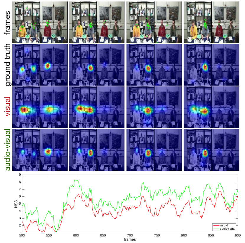
Figure 5: Sample frames from Coutrot2 database with their eye-tracking data, and the corresponding ground truth, spatio-temporal visual, and audiovisual saliency maps as produced by STAViS (visual-only and audiovisual). Also NSS curve for visual and audiovisual approaches is depicted.

Data Augmentation: The input samples in the network consist of 16-frames RGB video clips spatially resized at $112\times 112$ pixels, as well as the corresponding audio stream. We have also applied data augmentation for random generation of training samples. First, we divided the initial long-duration videos into 90-frame, non-overlapping segments and then generated the 16-frames from each segment by applying a random flipping process, as in [62], but without random cropping. We applied the same spatial transformations to the 16 frames of the video clip and the eye-tracking based saliency map of the median frame, which is considered the clip’s ground truth map.

Testing: During testing phase, we obtain an estimated saliency map per frame using a 16-frame sliding window with step 1 without any random flipping.

4 Experiments

	Overall
	CC $\uparrow$	NSS $\uparrow$	AUC-J $\uparrow$	sAUC $\uparrow$	SIM $\uparrow$
Visual	0.5260	2.54	0.8922	0.6187	0.4088
$L_{1}$_AudioOnly	0.5132	2.48	0.8923	0.6220	0.4100
$L_{2}$_AudioOnly	0.5381	2.63	0.8969	0.6171	0.4157
$L_{3}$_AudioOnly	0.5226	2.59	0.8935	0.6228	0.4027
$L_{1}$_$S_{1}^{av}$	0.5243	2.62	0.8924	0.6224	0.4103
$L_{2}$_$S_{1}^{av}$	0.5344	2.69	0.8944	0.6215	0.4249
$L_{3}$_$S_{1}^{av}$	0.5354	2.71	0.8959	0.6236	0.4278
$L_{1}$_$S_{2}^{av}$	0.5069	2.43	0.8687	0.6223	0.2985
$L_{2}$_$S_{2}^{av}$	0.5082	2.44	0.8699	0.6225	0.2996
$L_{3}$_$S_{2}^{av}$	0.5066	2.46	0.8622	0.6219	0.2981
$L_{3}^{mul}$_$\tilde{S}_{2}^{av}$	0.5271	2.56	0.8943	0.6242	0.4132
$\mathbf{L_{3}^{mul}}$_$\mathbf{S_{3}^{av}}$	0.5414	2.73	0.8983	0.6267	0.4241
$L_{3}^{mul}$_$S_{fus}^{av}$	0.5401	2.70	0.8979	0.6261	0.4290

Table 1: Ablation study: $L_{1},L_{2}$ and $L_{3}$ refer to the audio localization method: cosine, inner product and bilinear respectively. $S_{1}^{av},S_{2}^{av}$, $S_{3}^{av}$ and $S_{fus}^{av}$ refer to the different fusion methods. Superscript “mul” refers to multiple feature maps.

	DIEM					Coutrot1					Coutrot2
	CC $\uparrow$	NSS $\uparrow$	AUC-J $\uparrow$	sAUC $\uparrow$	SIM $\uparrow$	CC $\uparrow$	NSS $\uparrow$	AUC-J $\uparrow$	sAUC $\uparrow$	SIM $\uparrow$	CC $\uparrow$	NSS $\uparrow$	AUC-J $\uparrow$	sAUC $\uparrow$	SIM $\uparrow$
STAViS [STA]	0.5795	2.26	0.8838	0.6741	0.4824	0.4722	2.11	0.8686	0.5847	0.3935	0.7349	5.28	0.9581	0.7106	0.5111
STAViS [ST]	0.5665	2.19	0.8792	0.6648	0.4719	0.4587	1.99	0.8617	0.5764	0.3842	0.6529	4.19	0.9405	0.6895	0.4470
DeepNet [44] [S]	0.4075	1.52	0.8321	0.6227	0.3183	0.3402	1.41	0.8248	0.5597	0.2732	0.3012	1.82	0.8966	0.6000	0.2019
DVA [63] [S]	0.4779	1.97	0.8547	0.641	0.3785	0.4306	2.07	0.8531	0.5783	0.3324	0.4634	3.45	0.9328	0.6324	0.2742
SAM [11] [S]	0.4930	2.05	0.8592	0.6446	0.4261	0.4329	2.11	0.8571	0.5768	0.3672	0.4194	3.02	0.9320	0.6152	0.3041
SalGAN [43] [S]	0.4868	1.89	0.8570	0.6609	0.3931	0.4161	1.85	0.8536	0.5799	0.3321	0.4398	2.96	0.9331	0.6183	0.2909
ACLNet [64, 65] [ST]	0.5229	2.02	0.8690	0.6221	0.4279	0.4253	1.92	0.8502	0.5429	0.3612	0.4485	3.16	0.9267	0.5943	0.3229
DeepVS [25] [ST]	0.4523	1.86	0.8406	0.6256	0.3923	0.3595	1.77	0.8306	0.5617	0.3174	0.4494	3.79	0.9255	0.6469	0.2590
TASED [38] [ST]	0.5579	2.16	0.8812	0.6579	0.4615	0.4799	2.18	0.8676	0.5808	0.3884	0.4375	3.17	0.9216	0.6118	0.3142

Table 2: Evaluation results for saliency in DIEM, Coutrot1 and Coutrot2 databases. The proposed method’s (STAViS [STA]) results are depicted in the first row, while the second one refers to our visual-only version. In most cases, the proposed network outperforms the existing state-of-the-art methods for saliency estimation according the five evaluation metrics. [STA] stands for spatio-temporal audiovisual, [ST] for spatio-temporal visual models while [S] denotes a spatial only model that is applied to each frame independently.

	AVAD					SumMe					ETMD
	CC $\uparrow$	NSS $\uparrow$	AUC-J $\uparrow$	sAUC $\uparrow$	SIM $\uparrow$	CC $\uparrow$	NSS $\uparrow$	AUC-J $\uparrow$	sAUC $\uparrow$	SIM $\uparrow$	CC $\uparrow$	NSS $\uparrow$	AUC-J $\uparrow$	sAUC $\uparrow$	SIM $\uparrow$
STAViS [STA]	0.6086	3.18	0.9196	0.5936	0.4578	0.4220	2.04	0.8883	0.6562	0.3373	0.5690	2.94	0.9316	0.7317	0.4251
STAViS [ST]	0.6041	3.07	0.9157	0.5900	0.4431	0.4180	1.98	0.8848	0.6477	0.3325	0.5602	2.84	0.9290	0.7278	0.4121
DeepNet [44] [S]	0.3831	1.85	0.8690	0.5616	0.2564	0.3320	1.55	0.8488	0.6451	0.2274	0.3879	1.90	0.8897	0.6992	0.2253
DVA [63] [S]	0.5247	3.00	0.8887	0.5820	0.3633	0.3983	2.14	0.8681	0.6686	0.2811	0.4965	2.72	0.9039	0.7288	0.3165
SAM [11] [S]	0.5279	2.99	0.9025	0.5777	0.4244	0.4041	2.21	0.8717	0.6728	0.3272	0.5068	2.78	0.9073	0.7310	0.3790
SalGAN [43] [S]	0.4912	2.55	0.8865	0.5799	0.3608	0.3978	1.97	0.8754	0.6882	0.2897	0.4765	2.46	0.9035	0.7463	0.3117
ACLNet [64, 65] [ST]	0.5809	3.17	0.9053	0.5600	0.4463	0.3795	1.79	0.8687	0.6092	0.2965	0.4771	2.36	0.9152	0.6752	0.3290
DeepVS [25] [ST]	0.5281	3.01	0.8968	0.5858	0.3914	0.3172	1.62	0.8422	0.6120	0.2622	0.4616	2.48	0.9041	0.6861	0.3495
TASED [38] [ST]	0.6006	3.16	0.9146	0.5898	0.4395	0.4288	2.10	0.8840	0.6570	0.3337	0.5093	2.63	0.9164	0.7117	0.3660

Table 3: Evaluation results for audiovisual saliency in AVAD, SumMe and ETMD databases. The proposed method’s (STAViS [STA]) results are depicted in the first row, while the second one refers to our visual-only version. In most cases, the proposed network outperforms the existing state-of-the-art methods for saliency estimation according the five evaluation metrics. [STA] stands for spatio-temporal audiovisual, [ST] for spatio-temporal visual models while [S] denotes a spatial only model that is applied to each frame independently.

4.1 Datasets

In order to train and evaluate the proposed audiovisual saliency network, 6 different datasets are employed, containing audiovisual eye-tracking data: DIEM, AVAD, Coutrot1, Coutrot2, SumMe, and ETMD. These databases consist of various types of videos, ranging from very structured small videos to completely unstructured, user-made Youtube videos. Our goal is to train and evaluate the model using different types of audiovisual data, in order to obtain a good performance “in-the-wild” and help the model learn if and when it should use audio to enhance visual saliency. A short description for each database follows.

AVAD: AVAD database [39] contains 45 short clips of 5-10 sec duration with several audiovisual scenes, e.g. dancing, guitar playing, bird signing, etc. A joint audiovisual event per video is always present. Eye-tracking data from 16 participants have been recorded.

Coutrot databases: Coutrot databases [13, 14] are split in Coutrot1 and Coutrot2: Coutrot1 contains 60 clips with dynamic natural scenes split in 4 visual categories: one/several moving objects, landscapes, and faces. Eye-tracking data from 72 participants have been recorded. Coutrot2 contains 15 clips of 4 persons in a meeting and the corresponding eye-tracking data from 40 persons.

DIEM: DIEM database [41] consists of $84$ movies of all sorts, sourced from publicly accessible repositories, including advertisements, documentaries, game trailers, movie trailers, music videos, news clips, and time-lapse footage. Thus, the majority of DIEM videos are documentary-like, which means that audio and visual information do not correspond to the same event. Eye movement data from $42$ participants were recorded via an Eyelink eye-tracker, while watching the videos in random order and with the audio on.

SumMe: SumMe database [19, 58] contains $25$ unstructured videos, i.e. mostly user-made videos, as well as their corresponding multiple-human created summaries, which were acquired in a controlled psychological experiment. Audiovisual eye-tracking data have been collected [58] from $10$ viewers, recorded via an Eyelink eye-tracker.

ETMD: ETMD database [27, 58] contains $12$ videos from six different hollywood movies. Audiovisual eye-tracking data have been collected [58] from $10$ viewers, recorded via an Eyelink eye-tracker.

4.2 Experimental Results

Training has been performed by combining data from all datasets: For DIEM, the standard split from literature has been employed [5]. For the other 5 databases, where there is no particular split, we created 3 different splits of the data, in the sense of 3-fold cross-validation, with non-overlapping videos between train, validation and test sets for each split, uniformly split among datasets. Among these 3 different splits, different videos were placed in each split, namely, if video1 of dataset1 was placed in test set of split1, then it would not appear in any other test set. We ensured that all videos of each dataset would appear once in the test set of one split. The models’ final performance was obtained by taking the average among all 3 splits. The same procedure was carried out both for our audiovisual and visual variants, in order to ensure a fair comparison.

For the evaluation of STAViS network, we first investigate the performance of the various sound localization and fusion techniques described in Sec. 3. We pick the method with the best results and compare it to 8 state-of-the-art visual saliency methods (using their publicly available codes and models), in all 6 databases on the same test data. We employ five widely-used evaluation metrics for saliency [6]: CC, NSS, AUC-Judd (AUC-J), shuffled AUC (sAUC) and SIM (similarity). For sAUC we select the negative samples from the union of all viewers’ fixations across all other frames except the frame for which we compute the AUC.

Ablation study: Regarding Table 1, we can observe that bilinear transformation $L_{3}$ achieves better performance compared to the other sound localization methods since the latter can be consider as simpler versions of the bilinear function. Moreover, it can be noted that methods based only on audio localization can achieve quite high scores while they are further improved when fused with pure visual cues. Especially when multiple maps are fused with the visual ones by concatenation $S_{3}^{av}$, thus allowing for the most interaction between the features, the best performance is achieved in almost all metrics. Competitive performance is also achieved with late fusion, as indicated by the last row of Table 1. Overall, cosine similarity for localization $L_{1}$ performs worst in all cases, since it does not have any learnable parameters, while fusion scheme $S_{2}^{av}$ that has performed well in signal processing based methods [58] does not seem suitable for deep learning approaches. Thus, we pick up method $L_{3}^{mul}S_{3}^{av}$ as our proposed STAViS method. Figures 4, 5 depict some sample frames from Coutrot1 and Coutrot2 along with their corresponding eye-tracking data and the ground truth, visual-only (ours) and the STAViS saliency maps. Attention is much better captured by the proposed STAViS model. They also depict NSS curve over time for visualization and comparison purposes.

Comparisons with state-of-the-art: Next, we proceed with extensive comparisons with 8 different state-of-the-art saliency methods, depicted for the five metrics per database, in Tables 7, 8. Results highlight the superiority of our proposed audiovisual method, as it outperforms almost for all databases and metrics the other state-of-the-art methods. We can observe that all the other state-of-the-art methods, except for TASED, achieve good performance in some databases, but not consistently, meaning that they might perform well for particular types of video but not for all types. For example, ACLNet performs well for AVAD database but not equally well in SumMe which has more unstructured, home-made videos. TASED achieves good performance, even better than STAViS for CC and NSS in Coutrot1 and SumMe, but it does not perform equally well for Coutrot2. Overall, a good performance is achieved from our visual-only version as well.

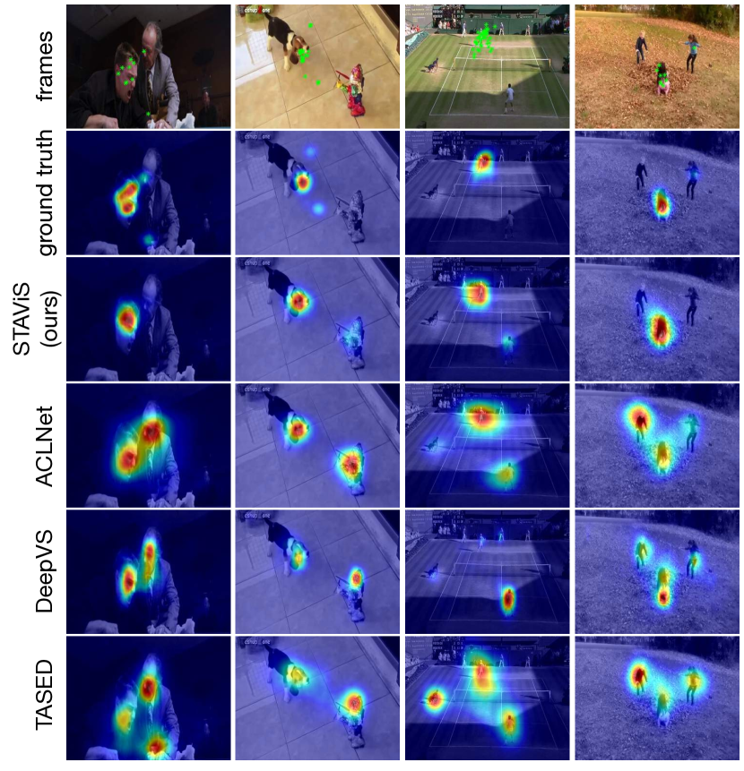
Figure 6: Sample frame from ETMD, AVAD, DIEM and SumMe databases with their eye-tracking data, and the corresponding ground truth, STAViS, and other spatio-temporal state-of-the-art visual saliency maps for comparisons.

Discussion: Our proposed spatio-temporal auditory saliency model STAViS performs consistently well across all datasets, achieving the best performance compared to state-of-the-art methods for almost all databases and metrics. It should be noted that these databases contain a large variety of videos types. From documentaries, where there is no audiovisual correspondence, to Hollywood movies and unprocessed user-made videos. Thus our model achieves a good performance “in-the-wild”, without any prior knowledge on the content of the video. This performance for this large range could indicate that our model is capable of learning if, where and when auditory saliency integration should be performed. In addition, especially in Coutrot2 that is the most “audiovisual” database in the sense that all included events/videos consist of audiovisual scenes, our model clearly outperforms the rest by a large margin probably because it better captures the audiovisual correspondences. For visualization purposes, in Fig. 6 a sample frame from ETMD, AVAD, DIEM and SumMe database is presented with its corresponding eye-tracking data in the first row. The second row depicts the ground truth saliency map. The third row includes the corresponding saliency maps from our STAViS model, while the final 3 rows, the same maps for ACLNet, DeepVS and TASED. It can easily be observed that our results are closer to the ground truth.

5 Conclusions

We have proposed STAViS, a novel spatio-temporal audiovisual network that efficiently addresses the problem of fixation prediction in videos, i.e. video saliency estimation. It employs an extended state-of-the-art visual saliency network, a state-of-the-art audio representation network and features a sound source localization module that produces one or multiple auditory saliency maps and a fusion module that combines auditory and visual saliency maps in order to produce an audiovisual saliency map. All components have been designed, trained end-to-end, and extensively evaluated in a variety of videos. Results for 5 different metrics in 6 different databases and comparison with 8 state-of-the-art methods indicate the appropriateness and efficiency of this audiovisual approach for saliency modeling.

6 Supplementary material

6.1 Configuration and parameters of the employed CNN architectures

In Tables 4, 5 we present the configuration and the parameters of the employed visual and audio sub-networks based on the 3D-ResNet-50 [20] and SounNet [3] architectures respectively. Figure 7 depicts the architecture of a 3D Bottleneck Block that constitutes the main building unit of the spatio-temporal 3D ResNet.

Layer	3D-Conv1	3D Max Pool	3D Conv2 Block	3D Conv3 Block	3D Conv4 Block
Number of feature maps ($F$)	64	64	64	128	256
Filter Kernel	$7\times 7\times 7$	$3\times 3\times 3$	Bottleneck	Bottleneck	Bottleneck
Stride	$7\times 7\times 1$	$2\times 2\times 2$	$1\times 1\times 1$	$2\times 2\times 2$	$2\times 2\times 2$
Number of Blocks	-	-	3	4	6

Table 4: Configuration and parameters of the 3D ResNet architecture that has been employed in the patio-temporal network for visual saliency.

Layer	Conv1	Pool1	Conv2	Pool2	Conv3	Conv4	Conv5	Pool5	Conv6	Conv7
Number of feature channels	16	16	32	32	64	128	256	256	512	1024
Filter Kernel	64	8	32	8	16	8	4	4	4	4
Stride	2	1	2	1	2	2	2	1	2	2
Padding	32	0	16	0	8	4	2	0	2	2

Table 5: Configuration and parameters of the Audio Representation Network.

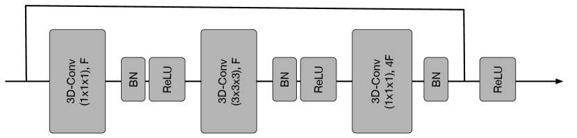
Figure 7: Architecture of the 3D Bottleneck Block. $F$ denotes the number of feature maps of the 3D convolutional filter while BN refers to batch normalization.

6.2 Data splits and training

6.2.1 Data splits

As mentioned in the main body of the paper, training has been performed by combining data from all datasets: For DIEM, the standard split from literature has been employed [5]. For the other 5 databases, where there is no particular split, we created 3 different splits of the data, in the sense of 3-fold cross-validation, with non-overlapping videos between train, validation and test sets for each split, uniformly split among datasets. Among these 3 different splits, different videos were placed in each split, namely, if video1 of dataset1 was placed in test set of split1, then it would not appear in any other test set. We ensured that all videos of each dataset would appear once in the test set of one split. The models’ final performance was obtained by taking the average among all 3 splits. The same procedure was carried out both for our audiovisual and visual variants, in order to ensure a fair comparison. In Table 6, the detailed list of the video contents of each split is depicted for completeness.

6.2.2 Training

In this subsection, the training process is described in more detail. First the visual-only network is trained, using as starting point the pretrained model in the Kinetics 400 database [20, 8] and employing DSAM skip connections. Afterwards, the whole audio-visual network is trained end-to-end, using the previously trained visual-only network as starting point for the visual path, while for the audio representation path we use as starting point the pretrained model from Flickr [3]. The network was trained either for 100 epochs or until loss did not further improve during 10 epochs, which usually happened around 60 epochs. Also, multi-step learning rate has been employed. The hyperparameters listed in the main body of the paper have mainly been decided upon experimentation.

	Test split 1	Test split 2	Test split 3
Database	video	video	video
AVAD	V32_Dancers	V22_Tap2	V40_Guitar5
AVAD	V6_Basketball1	V34_Beat	V16_Drummer2
AVAD	V33_Harp	V35_Squirrel	V30_Dog3
AVAD	V17_Soccer1	V3_Speech3	V7_Basketball2
AVAD	V41_Violin1	V11_News4	V42_Violin2
AVAD	V29_Dog2	V45_Darbuka2	V28_Dog1
AVAD	V25_Piano1	V38_Guitar3	V5_Interview2
AVAD	V31_Bird	V14_Conservation3	V21_Tap1
AVAD	V27_Piano3	V8_News1	V37_Guitar2
AVAD	V15_Drummer1	V44_Darbuka1	V26_Piano2
AVAD	V23_Tap3	V1_Speech1	V43_Violin3
AVAD	V24_Tap4	V36_Guitar1	V19_Singing1
AVAD	V13_Conservation2	V2_Speech2	V4_Interview1
AVAD	V9_News2	V18_Soccer2	V20_Singing2
AVAD	V10_News3	V39_Guitar4	V12_Conservation1
Coutrot 1	clip4	clip1	clip2
Coutrot 1	clip5	clip3	clip6
Coutrot 1	clip10	clip7	clip9
Coutrot 1	clip14	clip8	clip12
Coutrot 1	clip15	clip11	clip13
Coutrot 1	clip16	clip25	clip18
Coutrot 1	clip17	clip27	clip19
Coutrot 1	clip22	clip28	clip20
Coutrot 1	clip24	clip29	clip21
Coutrot 1	clip26	clip30	clip23
Coutrot 1	clip32	clip31	clip34
Coutrot 1	clip37	clip33	clip35
Coutrot 1	clip38	clip36	clip40
Coutrot 1	clip39	clip42	clip41
Coutrot 1	clip44	clip43	clip45
Coutrot 1	clip47	clip49	clip46
Coutrot 1	clip48	clip52	clip51
Coutrot 1	clip50	clip54	clip53
Coutrot 1	clip56	clip55	clip59
Coutrot 1	clip58	clip57	clip60
Coutrot2	clip4	clip12	clip3
Coutrot2	clip15	clip13	clip1
Coutrot2	clip11	clip10	clip9
Coutrot2	clip14	clip7	clip6
Coutrot2	clip2	clip5	clip8
DIEM	BBC_life_in_cold_blood	BBC_life_in_cold_blood	BBC_life_in_cold_blood
DIEM	BBC_wildlife_serpent	BBC_wildlife_serpent	BBC_wildlife_serpent
DIEM	DIY_SOS	DIY_SOS	DIY_SOS
DIEM	advert_bbc4_bees	advert_bbc4_bees	advert_bbc4_bees
DIEM	advert_bbc4_library	advert_bbc4_library	advert_bbc4_library
DIEM	advert_iphone	advert_iphone	advert_iphone
DIEM	ami_ib4010_closeup	ami_ib4010_closeup	ami_ib4010_closeup
DIEM	ami_ib4010_left	ami_ib4010_left	ami_ib4010_left
DIEM	harry_potter_6_trailer	harry_potter_6_trailer	harry_potter_6_trailer
DIEM	music_gummybear	music_gummybear	music_gummybear
DIEM	music_trailer_nine_inch_nails	music_trailer_nine_inch_nails	music_trailer_nine_inch_nails
DIEM	news_tony_blair_resignation	news_tony_blair_resignation	news_tony_blair_resignation
DIEM	nightlife_in_mozambique	nightlife_in_mozambique	nightlife_in_mozambique

DIEM	one_show	one_show	one_show
DIEM	pingpong_angle_shot	pingpong_angle_shot	pingpong_angle_shot
DIEM	pingpong_no_bodies	pingpong_no_bodies	pingpong_no_bodies
DIEM	sport_scramblers	sport_scramblers	sport_scramblers
DIEM	sport_wimbledon_federer_final	sport_wimbledon_federer_final	sport_wimbledon_federer_final
DIEM	tv_uni_challenge_final	tv_uni_challenge_final	tv_uni_challenge_final
DIEM	university_forum_construction_ionic	university_forum_construction_ionic	university_forum_construction_ionic
SumMe	Valparaiso_Downhill	Cooking	Base_jumping
SumMe	Car_railcrossing	Bus_in_Rock_Tunnel	Bike_Polo
SumMe	Bearpark_climbing	Uncut_Evening_Flight	Scuba
SumMe	Playing_on_water_slide	playing_ball	paluma_jump
SumMe	Fire_Domino	St_Maarten_Landing	Kids_playing_in_leaves
SumMe	Cockpit_Landing	Paintball	Eiffel_Tower
SumMe	Saving_dolphines	Air_Force_One	Statue_of_Liberty
SumMe	Notre_Dame	car_over_camera	Excavators_river_crossing
SumMe			Jumps
ETMD	CHI_1_color	CRA_1_color	DEP_1_color
ETMD	CHI_2_color	CRA_2_color	DEP_2_color
ETMD	GLA_1_color	FNE_1_color	LOR_1_color
ETMD	GLA_2_color	FNE_2_color	LOR_2_color

Table 6: Detailed list of the video contents of each one of the three test splits. Note that regarding DIEM, the same videos are contained in every split, because there is a specific train, validation and test split from the literature.

6.3 Ablation study per database

Due to space restrictions, in the main body of the paper paper, the ablation study was presented as a table summarizing the results for all the videos contained in the employed databases. Here, in Tables 7,8 the ablation study results and the state-of-the-art evaluation results have been concatenated and presented per database for completeness. For details about the state-of-the-art methods please refer to the main paper.

We notice that except for a few cases, audiovisual combinations outperform all other visual-only methods, including our visual only variant. Sometimes, the performance is better by a large margin, as for example in Coutrot2, which is the most “audiovisual” database. In Coutrot2, all audiovisual combinations outperform the visual-only by far, indicating that the network indeed learns to fuse auditory saliency in order to predict fixations closer to the human ones.

An interesting remark concerns SumMe database, which contains the most unedited, user-made videos. Many of its videos include footages, GoPro cameras, videos with artificial sound, etc., thus, the majority does not contain many actual audiovisual events. However, audiovisual methods have performed quite well. Surprisingly though, the best performance in 3 out of 5 metrics is achieved by an audio-only method, that localizes the sound source among the other redundant information included in SumMe videos. Regarding the rest 2 metrics, the best performance is achieved by two different state-of-the-art spatial-only visual saliency methods.

6.4 Video demos of the proposed STAViS Network

In the supplementary material folder we have also included 4 demo videos (which correspond to the figures of the main body of the paper) that demonstrate better our approach over several video from all the employed databases.

	DIEM					Coutrot1					Coutrot2
	CC $\uparrow$	NSS $\uparrow$	AUC-J $\uparrow$	sAUC $\uparrow$	SIM $\uparrow$	CC $\uparrow$	NSS $\uparrow$	AUC-J $\uparrow$	sAUC $\uparrow$	SIM $\uparrow$	CC $\uparrow$	NSS $\uparrow$	AUC-J $\uparrow$	sAUC $\uparrow$	SIM $\uparrow$
Visual	0.5665	2.19	0.8792	0.6648	0.4719	0.4587	1.99	0.8617	0.5764	0.3842	0.6529	4.19	0.9405	0.6895	0.4470
$L_{1}$_AudioOnly	0.5362	2.05	0.8719	0.6596	0.4573	0.4444	1.93	0.8605	0.5789	0.3813	0.6917	4.67	0.9519	0.7013	0.4970
$L_{2}$_AudioOnly	0.5458	2.10	0.8737	0.6601	0.4569	0.4687	2.04	0.8669	0.584	0.3880	0.7223	4.99	0.9572	0.7054	0.5000
$L_{3}$_AudioOnly	0.5407	2.10	0.8719	0.6594	0.4552	0.4491	1.99	0.8618	0.5799	0.3745	0.7126	4.96	0.9568	0.7023	0.4849
$L_{1}$_$S_{1}^{av}$	0.5489	2.13	0.8743	0.6582	0.4623	0.4516	2.01	0.8612	0.5803	0.3808	0.7102	5.01	0.9523	0.7023	0.4911
$L_{2}$_$S_{1}^{av}$	0.5731	2.25	0.8839	0.6701	0.4847	0.4577	2.04	0.8602	0.5770	0.3892	0.7040	5.02	0.9480	0.6954	0.5017
$L_{3}$_$S_{1}^{av}$	0.5712	2.25	0.8825	0.6693	0.4848	0.4623	2.07	0.8649	0.5820	0.3934	0.7076	5.08	0.9499	0.7003	0.5112
$L_{1}$_$S_{2}^{av}$	0.525	2.04	0.8367	0.661	0.3519	0.4437	1.91	0.8354	0.5787	0.2994	0.6250	3.90	0.9168	0.6958	0.2785
$L_{2}$_$S_{2}^{av}$	0.5259	2.04	0.8376	0.6607	0.3527	0.4448	1.92	0.8374	0.5789	0.3005	0.6257	3.90	0.9171	0.6952	0.2801
$L_{3}$_$S_{2}^{av}$	0.5309	2.07	0.8344	0.6648	0.3553	0.4364	1.90	0.8218	0.5782	0.2924	0.6309	4.07	0.9161	0.6977	0.2883
$L_{3}^{mul}$_$\tilde{S}_{2}^{av}$	0.5594	2.14	0.8785	0.6681	0.4694	0.4588	2.00	0.8633	0.5823	0.3872	0.6983	4.70	0.9513	0.7035	0.4762
$\mathbf{L_{3}^{mul}}$_$\mathbf{S_{3}^{av}}$ (proposed)	0.5795	2.26	0.8838	0.6741	0.4824	0.4722	2.11	0.8686	0.5847	0.3935	0.7349	5.28	0.9581	0.7106	0.5111
$L_{3}^{mul}$_$S_{fus}^{av}$	0.5795	2.25	0.8843	0.6727	0.4877	0.4679	2.08	0.8670	0.5835	0.3954	0.7215	5.10	0.9551	0.7083	0.5137
DeepNet [44]	0.4075	1.52	0.8321	0.6227	0.3183	0.3402	1.41	0.8248	0.5597	0.2732	0.3012	1.82	0.8966	0.6000	0.2019
DVA [63]	0.4779	1.97	0.8547	0.641	0.3785	0.4306	2.07	0.8531	0.5783	0.3324	0.4634	3.45	0.9328	0.6324	0.2742
SAM [11]	0.4930	2.05	0.8592	0.6446	0.4261	0.4329	2.11	0.8571	0.5768	0.3672	0.4194	3.02	0.9320	0.6152	0.3041
SalGAN [pan2017salgan]	0.4868	1.89	0.8570	0.6609	0.3931	0.4161	1.85	0.8536	0.5799	0.3321	0.4398	2.96	0.9331	0.6183	0.2909
ACLNet [64, 65]	0.5229	2.02	0.8690	0.6221	0.4279	0.4253	1.92	0.8502	0.5429	0.3612	0.4485	3.16	0.9267	0.5943	0.3229
DeepVS [25]	0.4523	1.86	0.8406	0.6256	0.3923	0.3595	1.77	0.8306	0.5617	0.3174	0.4494	3.79	0.9255	0.6469	0.2590
TASED [38]	0.5579	2.16	0.8812	0.6579	0.4615	0.4799	2.18	0.8676	0.5808	0.3884	0.4375	3.17	0.9216	0.6118	0.3142

Table 7: Ablation study and state-of-the-art evaluation for databases DIEM, Coutrot1 and Coutrot2.

	AVAD					SumMe					ETMD
	CC $\uparrow$	NSS $\uparrow$	AUC-J $\uparrow$	sAUC $\uparrow$	SIM $\uparrow$	CC $\uparrow$	NSS $\uparrow$	AUC-J $\uparrow$	sAUC $\uparrow$	SIM $\uparrow$	CC $\uparrow$	NSS $\uparrow$	AUC-J $\uparrow$	sAUC $\uparrow$	SIM $\uparrow$
Visual	0.6041	3.07	0.9157	0.5900	0.4431	0.4180	1.98	0.8848	0.6477	0.3325	0.5602	2.84	0.9290	0.7278	0.4121
$L_{1}$_AudioOnly	0.5836	2.89	0.9176	0.5949	0.4413	0.4072	1.93	0.8833	0.6520	0.3328	0.5407	2.71	0.9276	0.7298	0.4086
$L_{2}$_AudioOnly	0.6107	3.07	0.9199	0.5975	0.4475	0.4413	2.12	0.8908	0.6665	0.3442	0.5580	2.84	0.9302	0.7343	0.4087
$L_{3}$_AudioOnly	0.6009	3.07	0.9185	0.5956	0.4351	0.4097	1.95	0.8838	0.6527	0.3218	0.5504	2.81	0.9285	0.7301	0.3995
$L_{1}$_$S_{1}^{av}$	0.6035	3.13	0.9166	0.5984	0.4463	0.4069	1.94	0.8826	0.6463	0.3271	0.5493	2.82	0.9277	0.7264	0.4073
$L_{2}$_$S_{1}^{av}$	0.6198	3.26	0.9201	0.5949	0.4700	0.4146	2.01	0.8872	0.6514	0.3359	0.5599	2.90	0.9303	0.7256	0.4238
$L_{3}$_$S_{1}^{av}$	0.6159	3.25	0.9195	0.5934	0.4690	0.4136	1.99	0.8856	0.6520	0.3391	0.5658	2.93	0.9312	0.7292	0.4296
$L_{1}$_$S_{2}^{av}$	0.5886	2.96	0.9013	0.5951	0.3156	0.4035	1.91	0.8618	0.6540	0.2470	0.5418	2.74	0.911	0.7346	0.2773
$L_{2}$_$S_{2}^{av}$	0.5912	2.98	0.9021	0.5957	0.3172	0.4038	1.91	0.8627	0.6542	0.2476	0.5423	2.74	0.9116	0.7346	0.2784
$L_{3}$_$S_{2}^{av}$	0.5860	2.96	0.8899	0.5947	0.3036	0.4110	1.97	0.8710	0.6513	0.2620	0.5530	2.86	0.9161	0.7311	0.3070
$L_{3}^{mul}$_$\tilde{S}_{2}^{av}$	0.5966	2.98	0.9179	0.5914	0.4449	0.4188	1.99	0.8853	0.6566	0.3358	0.5551	2.80	0.9292	0.7333	0.4136
$\mathbf{L_{3}^{mul}}$_$\mathbf{S_{3}^{av}}$ (proposed)	0.6086	3.18	0.9196	0.5936	0.4578	0.4220	2.03	0.8883	0.6562	0.3373	0.5690	2.93	0.9316	0.7317	0.4251
$L_{3}^{mul}$_$S_{fus}^{av}$	0.6162	3.21	0.9216	0.5952	0.4690	0.4183	2.01	0.8871	0.6547	0.3403	0.5669	2.91	0.9317	0.7318	0.4280
DeepNet [44]	0.3831	1.85	0.8690	0.5616	0.2564	0.3320	1.55	0.8488	0.6451	0.2274	0.3879	1.90	0.8897	0.6992	0.2253
DVA [63]	0.5247	3.00	0.8887	0.5820	0.3633	0.3983	2.14	0.8681	0.6686	0.2811	0.4965	2.72	0.9039	0.7288	0.3165
SAM [11]	0.5279	2.99	0.9025	0.5777	0.4244	0.4041	2.21	0.8717	0.6728	0.3272	0.5068	2.78	0.9073	0.7310	0.3790
SalGAN [pan2017salgan]	0.4912	2.55	0.8865	0.5799	0.3608	0.3978	1.97	0.8754	0.6882	0.2897	0.4765	2.46	0.9035	0.7463	0.3117
ACLNet [64, 65]	0.5809	3.17	0.9053	0.5600	0.4463	0.3795	1.79	0.8687	0.6092	0.2965	0.4771	2.36	0.9152	0.6752	0.3290
DeepVS [25]	0.5281	3.01	0.8968	0.5858	0.3914	0.3172	1.62	0.8422	0.6120	0.2622	0.4616	2.48	0.9041	0.6861	0.3495
TASED [38]	0.6006	3.16	0.9146	0.5898	0.4395	0.4288	2.10	0.8840	0.6570	0.3337	0.5093	2.63	0.9164	0.7117	0.3660

Table 8: Ablation study and state-of-the-art evaluation for databases AVAD, SumMe and ETMD.

References

- [1] Relja Arandjelovic and Andrew Zisserman. Look, listen and learn. In Proc. IEEE Int. Conf. on Computer Vision (ICCV), pages 609–617, 2017.
- [2] Relja Arandjelovic and Andrew Zisserman. Objects that sound. In Proc. European Conf. on Computer Vision (ECCV), pages 435–451, 2018.
- [3] Yusuf Aytar, Carl Vondrick, and Antonio Torralba. Soundnet: Learning sound representations from unlabeled video. In Proc. Advances in Neural Information Processing Systems (NIPS), pages 892–900, 2016.
- [4] Cagdas Bak, Aysun Kocak, Erkut Erdem, and Aykut Erdem. Spatio-temporal saliency networks for dynamic saliency prediction. IEEE Trans. Multimedia, 20(7):1688–1698, 2018.
- [5] A. Borji, D. N. Sihite, and L. Itti. Quantitative analysis of human-model agreement in visual saliency modeling: A comparative study. IEEE Trans. Image Process., 22(1):55–69, 2013.
- [6] Zoya Bylinskii, Tilke Judd, Aude Oliva, Antonio Torralba, and Frédo Durand. What do different evaluation metrics tell us about saliency models? arXiv preprint arXiv:1604.03605, 2016.
- [7] Sergi Caelles, Kevis-Kokitsi Maninis, Jordi Pont-Tuset, Laura Leal-Taixé, Daniel Cremers, and Luc Van Gool. One-shot video object segmentation. In Proc. IEEE Conf. on Computer Vision and Pattern Recognition (CVPR), 2017.
- [8] Joao Carreira and Andrew Zisserman. Quo vadis, action recognition? a new model and the kinetics dataset. In Proc. IEEE Conf. on Computer Vision and Pattern Recognition (CVPR), 2017.
- [9] Yanxiang Chen, Tam V Nguyen, Mohan S Kankanhalli, Jun Yuan, Shuicheng Yan, and Meng Wang. Audio matters in visual attention. IEEE Trans. Circuits Syst. Video Technol., 24(11):1992–2003, 2014.
- [10] Chung-Cheng Chiu, Tara N Sainath, Yonghui Wu, Rohit Prabhavalkar, Patrick Nguyen, Zhifeng Chen, Anjuli Kannan, Ron J Weiss, Kanishka Rao, Ekaterina Gonina, et al. State-of-the-art speech recognition with sequence-to-sequence models. In Proc. IEEE Int. Conf. Acous., Speech, and Signal Processing (ICASSP), pages 4774–4778. IEEE, 2018.
- [11] Marcella Cornia, Lorenzo Baraldi, Giuseppe Serra, and Rita Cucchiara. Predicting Human Eye Fixations via an LSTM-based Saliency Attentive Model. IEEE Trans. Image Process., 27(10):5142–5154, 2018.
- [12] Antoine Coutrot and Nathalie Guyader. An audiovisual attention model for natural conversation scenes. In Proc. IEEE Int. Conf. on Image Processing (ICIP), pages 1100–1104, 2014.
- [13] Antoine Coutrot and Nathalie Guyader. How saliency, faces, and sound influence gaze in dynamic social scenes. Journal of Vision, 14(8):1–17, 2014.
- [14] Antoine Coutrot and Nathalie Guyader. Multimodal saliency models for videos. In Matei Mancas, Vincent P. Ferrera, Nicolas Riche, and John G. Taylor, editors, From Human Attention to Computational Attention: A Multidisciplinary Approach, pages 291–304. Springer New York, 2016.
- [15] Tung Dang, Christos Papachristos, and Kostas Alexis. Visual saliency-aware receding horizon autonomous exploration with application to aerial robotics. In IEEE Int. Conf. on Robotics and Automation (ICRA), pages 2526–2533. IEEE, 2018.
- [16] Georgios Evangelopoulos, Athanasia Zlatintsi, Alexandros Potamianos, Petros Maragos, Konstantinos Rapantzikos, Georgios Skoumas, and Yannis Avrithis. Multimodal saliency and fusion for movie summarization based on aural, visual, textual attention. IEEE Trans. Multimedia, 15(7):1553–1568, Nov. 2013.
- [17] Siavash Gorji and James J. Clark. Going from image to video saliency: Augmenting image salience with dynamic attentional push. In Proc. IEEE Conf. on Computer Vision and Pattern Recognition (CVPR), 2018.
- [18] Alex Graves, Abdel-rahman Mohamed, and Geoffrey Hinton. Speech recognition with deep recurrent neural networks. In Proc. IEEE Int. Conf. Acous., Speech, and Signal Processing (ICASSP), pages 6645–6649. IEEE, 2013.
- [19] Michael Gygli, Helmut Grabner, Hayko Riemenschneider, and Luc Van Gool. Creating summaries from user videos. In Proc. European Conf. on Computer Vision (ECCV), pages 505–520, 2014.
- [20] Kensho Hara, Hirokatsu Kataoka, and Yutaka Satoh. Can spatiotemporal 3d cnns retrace the history of 2d cnns and imagenet. In Proc. IEEE Conf. on Computer Vision and Pattern Recognition (CVPR), 2018.
- [21] Kaiming He, Georgia Gkioxari, Piotr Dollár, and Ross B. Girshick. Mask R-CNN. In Proc. IEEE Int. Conf. on Computer Vision (ICCV), 2017.
- [22] Kaiming He, Xiangyu Zhang, Shaoqing Ren, and Jian Sun. Deep residual learning for image recognition. In Proc. IEEE Conf. on Computer Vision and Pattern Recognition (CVPR), 2016.
- [23] Xun Huang, Chengyao Shen, Xavier Boix, and Qi Zhao. Salicon: Reducing the semantic gap in saliency prediction by adapting deep neural networks. In Proc. IEEE Int. Conf. on Computer Vision (ICCV), pages 262–270, 2015.
- [24] Saumya Jetley, Naila Murray, and Eleonora Vig. End-to-end saliency mapping via probability distribution prediction. In Proc. IEEE Conf. on Computer Vision and Pattern Recognition (CVPR), pages 5753–5761, 2016.
- [25] Lai Jiang, Mai Xu, Tie Liu, Minglang Qiao, and Zulin Wang. Deepvs: A deep learning based video saliency prediction approach. In Proc. European Conf. on Computer Vision (ECCV). 2018.
- [26] Bruno Korbar, Du Tran, and Lorenzo Torresani. Cooperative learning of audio and video models from self-supervised synchronization. In Advances in Neural Information Processing Systems, pages 7763–7774, 2018.
- [27] Petros Koutras and Petros Maragos. A perceptually based spatio-temporal computational framework for visual saliency estimation. Signal Process.: Image Communication, 38:15–31, 2015.
- [28] Petros Koutras and Petros Maragos. Susinet: See, understand and summarize it. In Proc. IEEE Conf. on Computer Vision and Pattern Recognition Workshop (CVPRW), 2019.
- [29] Petros Koutras, Georgia Panagiotaropoulou, Antigoni Tsiami, and Petros Maragos. Audio-visual temporal saliency modeling validated by fmri data. In Proc. IEEE Conf. on Computer Vision and Pattern Recognition Workshop (CVPRW), pages 2000–2010, 2018.
- [30] Gábor Kovács, Yasuharu Kunii, Takao Maeda, and Hideki Hashimoto. Saliency and spatial information-based landmark selection for mobile robot navigation in natural environments. Advanced Robotics, 33(10):520–535, 2019.
- [31] Matthias Kümmerer, Lucas Theis, and Matthias Bethge. Deep gaze I: Boosting saliency prediction with feature maps trained on imagenet. In Int. Conf. on Learning Representations Workshops (ICLRW), 2015.
- [32] Qiuxia Lai, Wenguan Wang, Hanqiu Sun, and Jianbing Shen. Video saliency prediction using spatiotemporal residual attentive networks. IEEE Trans. Image Process., 29:1113–1126, 2019.
- [33] George Leifman, Dmitry Rudoy, Tristan Swedish, Eduardo Bayro-Corrochano, and Ramesh Raskar. Learning gaze transitions from depth to improve video saliency estimation. In Proc. IEEE Int. Conf. on Computer Vision (ICCV), 2017.
- [34] Panagiotis Linardos, Eva Mohedano, Juan Jose Nieto, Kevin McGuinness, Xavier Giro-i Nieto, and Noel E. O’Connor. Simple vs complex temporal recurrences for video saliency prediction. In British Machine Vision Conf. (BMVC), 2019.
- [35] Harry McGurk and John MacDonald. Hearing lips and seeing voices. Nature, 264:746–748, 1976.
- [36] M Alex Meredith and Barry E Stein. Interactions among converging sensory inputs in the superior colliculus. Science, 221(4608):389–391, 1983.
- [37] M Alex Meredith and Barry E Stein. Visual, auditory, and somatosensory convergence on cells in superior colliculus results in multisensory integration. Journal of Neurophysiology, 56(3):640–662, 1986.
- [38] Kyle Min and Jason J. Corso. Tased-net: Temporally-aggregating spatial encoder-decoder network for video saliency detection. In Proc. IEEE Int. Conf. on Computer Vision (ICCV), pages 2394–2403, 2019.
- [39] Xiongkuo Min, Guangtao Zhai, Ke Gu, and Xiaokang Yang. Fixation prediction through multimodal analysis. ACM Transactions on Multimedia Computing, Communications, and Applications, 13(1), 2017.
- [40] Xiongkuo Min, Guangtao Zhai, Chunjia Hu, and Ke Gu. Fixation prediction through multimodal analysis. In Proc. IEEE Int. Conf. on Visual Communications and Image Processing, 2015.
- [41] Parag K. Mital, Tim J. Smith, Robin Hill, and John M. Henderson. Clustering of gaze during dynamic scene viewing is predicted by motion. Cognitive Computation, 3(1):5–24, 2011.
- [42] Andrew Owens and Alexei A Efros. Audio-visual scene analysis with self-supervised multisensory features. In Proc. European Conf. on Computer Vision (ECCV), pages 631–648, 2018.
- [43] Junting Pan, Cristian Canton, Kevin McGuinness, Noel E. O’Connor, Jordi Torres, Elisa Sayrol, and Xavier Giro-i Nieto. Salgan: Visual saliency prediction with generative adversarial networks. In Proc. IEEE Conf. on Computer Vision and Pattern Recognition Workshop (CVPRW), 2017.
- [44] Junting Pan, Elisa Sayrol, Xavier Giro-i Nieto, Kevin McGuinness, and Noel E. O’Connor. Shallow and deep convolutional networks for saliency prediction. In Proc. IEEE Conf. on Computer Vision and Pattern Recognition (CVPR), pages 598–606, 2016.
- [45] Paul Primus, Hamid Eghbal-zadeh, David Eitelsebner, Khaled Koutini, Andreas Arzt, and Gerhard Widmer. Exploiting parallel audio recordings to enforce device invariance in cnn-based acoustic scene classification. arXiv preprint arXiv:1909.02869, 2019.
- [46] Sudarshan Ramenahalli, Daniel R Mendat, Salvador Dura-Bernal, Eugenio Culurciello, Ernst Niebur, and Andreas Andreou. Audio-visual saliency map: Overview, basic models and hardware implementation. In Proc. Information Sciences and Systems (CISS), pages 1–6, 2013.
- [47] Rémi Ratajczak, Denis Pellerin, Quentin Labourey, and Catherine Garbay. A fast audiovisual attention model for human detection and localization on a companion robot. In Int. Conf. on Applications and Systems of Visual Paradigms, 2016.
- [48] Jamie Ray, Heng Wang, Du Tran, Yufei Wang, Matt Feiszli, Lorenzo Torresani, and Manohar Paluri. Scenes-objects-actions: A multi-task, multi-label video dataset. In Proc. European Conf. on Computer Vision (ECCV), 2018.
- [49] Jonas Ruesch, Manuel Lopes, Alexandre Bernardino, Jonas Hornstein, José Santos-Victor, and Rolf Pfeifer. Multimodal saliency-based bottom-up attention a framework for the humanoid robot iCub. In IEEE Int. Conf. on Robotics and Automation (ICRA), pages 962–967, 2008.
- [50] Boris Schauerte, Benjamin Kühn, Kristian Kroschel, and Rainer Stiefelhagen. Multimodal saliency-based attention for object-based scene analysis. In IEEE Int. Conf. on Intelligent Robots and Systems (IROS), pages 1173–1179. IEEE, 2011.
- [51] Arda Senocak, Tae-Hyun Oh, Junsik Kim, Ming-Hsuan Yang, and In So Kweon. Learning to localize sound source in visual scenes. In Proc. IEEE Conf. on Computer Vision and Pattern Recognition (CVPR), 2018.
- [52] Naty Sidaty, Mohamed-Chaker Larabi, and Abdelhakim Saadane. Toward an audiovisual attention model for multimodal video content. Neurocomputing, pages 94–111, 2017.
- [53] Karen Simonyan and Andrew Zisserman. Very deep convolutional networks for large-scale image recognition. In Int. Conf. on Learning Representations (ICLR), 2015.
- [54] Vincent Sitzmann, Ana Serrano, Amy Pavel, Maneesh Agrawala, Diego Gutierrez, Belen Masia, and Gordon Wetzstein. Saliency in vr: How do people explore virtual environments? IEEE Trans. Visualiz. Comp. Graphics, 24(4):1633–1642, 2018.
- [55] Guanghan Song. Effect of sound in videos on gaze: Contribution to audio-visual saliency modeling. PhD thesis, Universite de Grenoble, 2013.
- [56] Hamed R Tavakoli, Ali Borji, Esa Rahtu, and Juho Kannala. Dave: A deep audio-visual embedding for dynamic saliency prediction. arXiv preprint arXiv:1905.10693, 2019.
- [57] Yapeng Tian, Jing Shi, Bochen Li, Zhiyao Duan, and Chenliang Xu. Audio-visual event localization in unconstrained videos. In Proc. European Conf. on Computer Vision (ECCV), pages 247–263, 2018.
- [58] Antigoni Tsiami, Petros Koutras, Athanasios Katsamanis, Argiro Vatakis, and Petros Maragos. A behaviorally inspired fusion approach for computational audiovisual saliency modeling. Signal Processing: Image Communication, 76:186 – 200, 2019.
- [59] Erik Van der Burg, Christian NL Olivers, Adelbert W Bronkhorst, and Jan Theeuwes. Pip and pop: Nonspatial auditory signals improve spatial visual search. Journal of Experimental Psychology: Human Perception and Performance, 34:1053–1065, 2008.
- [60] Argiro Vatakis and Charles Spence. Crossmodal binding: Evaluating the “unity assumption” using audiovisual speech stimuli. Perception & Psychophysics, 69(5):744–756, 2007.
- [61] Eleonora Vig, Michael Dorr, and David Cox. Large-scale optimization of hierarchical features for saliency prediction in natural images. In Proc. IEEE Conf. on Computer Vision and Pattern Recognition (CVPR), pages 2798–2805, 2014.
- [62] Limin Wang, Yuanjun Xiong, Zhe Wang, Yu Qiao, Dahua Lin, Xiaoou Tang, and Luc Van Gool. Temporal segment networks: Towards good practices for deep action recognition. In Proc. European Conf. on Computer Vision (ECCV), pages 20–36, 2016.
- [63] Wenguan Wang and Jianbing Shen. Deep visual attention prediction. IEEE Trans. Image Process., 27(5):2368–2378, 2018.
- [64] Wenguan Wang, Jianbing Shen, Fang Guo, Ming-Ming Cheng, and Ali Borji. Revisiting video saliency: A large-scale benchmark and a new model. In Proc. IEEE Conf. on Computer Vision and Pattern Recognition (CVPR), 2018.
- [65] Wenguan Wang, Jianbing Shen, Jianwen Xie, Ming-Ming Cheng, Haibin Ling, and Ali Borji. Revisiting video saliency prediction in the deep learning era. IEEE Trans. Pattern Anal. Mach. Intell. (PAMI), pages 1–17, 2019.
- [66] Saining Xie and Zhuowen Tu. Holistically-nested edge detection. In Proc. IEEE Int. Conf. on Computer Vision (ICCV), 2015.
- [67] Xia Yuan, Juan Yue, and Yanan Zhang. Rgb-d saliency detection: Dataset and algorithm for robot vision. In 2018 IEEE Int. Conf. on Robotics and Biomimetics (ROBIO), pages 1028–1033. IEEE, 2018.
- [68] Hang Zhao, Chuang Gan, Wei-Chiu Ma, and Antonio Torralba. The sound of motions. In Proc. IEEE Int. Conf. on Computer Vision (ICCV), pages 1735–1744, 2019.
- [69] Hang Zhao, Chuang Gan, Andrew Rouditchenko, Carl Vondrick, Josh McDermott, and Antonio Torralba. The sound of pixels. In Proc. European Conf. on Computer Vision (ECCV), pages 570–586, 2018.