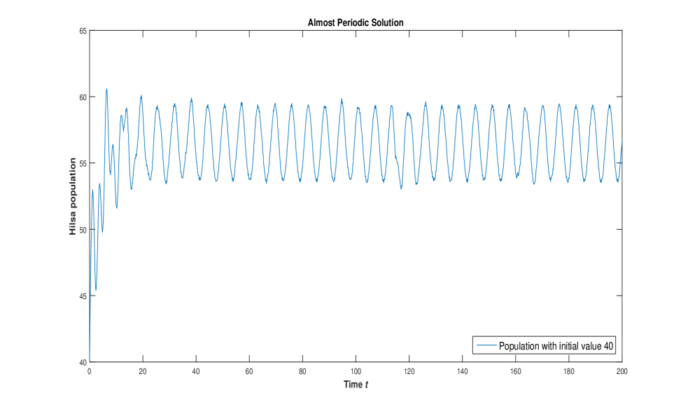
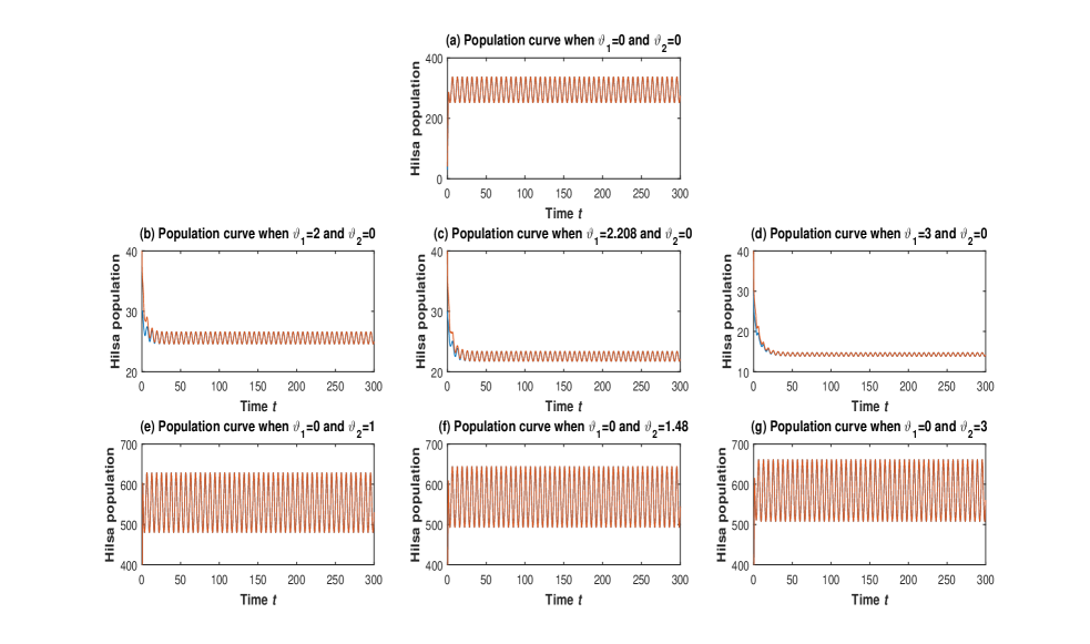
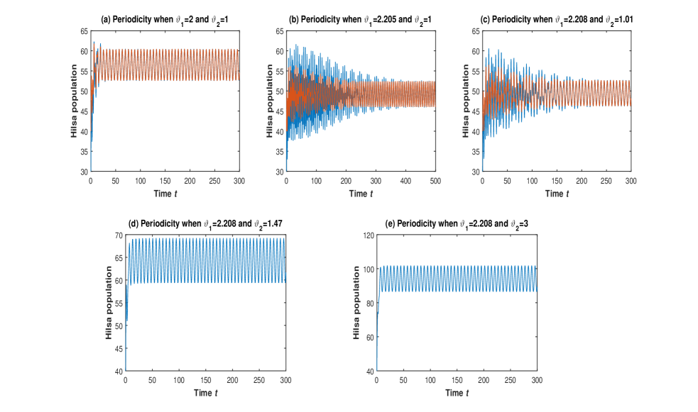
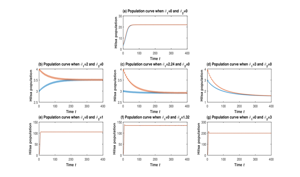
Abstract

This paper is concerned with an analysis of the dynamics of a non-autonomous, single population age based growth model with harvesting formulation. First, we derive sufficient conditions for permanence and positive invariance. Then, by constructing a scalar function, namely the Lyapunov function, we arrive at a suitable criterion for global attractivity. With the help of Brouwer fixed point and continuation theorems, we obtain constraints for the existence of a positive periodic solution. Then we prove that there exists only one solution which is almost periodic in nature that is distinct from every other solution. Further, we carry out a numerical simulation to support the analytical findings.

Keywords and phrases: Non-autonomous dynamical system, Age-structured model, Permanence, Periodic solution, Global attractivity, Almost periodic solution

AMS subject classifications: 37B55, 92D25, 92D40

Interplay between reproduction and age selective harvesting delays of a single population non-autonomous system

N. S. N. V. K. Vyshnavi Devi1, Debaldev Jana1,† and M. Lakshmanan2

1Department of Mathematics & SRM Research Institute,

SRM Institute of Science and Technology, Kattankulathur-603 203, Tamil Nadu, India.

E-mail: vyshu__\textunderscorenandi@ymail.com1 and debaldevjana.jana@gmail.com1,†

2Centre for Nonlinear Dynamics,

School of Physics, Bharathidasan University, Tiruchirapalli - 620 024, India.

E-mail: lakshman.cnld@gmail.com2

1 Introduction

Population dynamics speaks about the changes that occur in a given population as it varies with time, due to factors like birth, death, and migration. It acts as the fundamental principle for interpreting various patterns in fishery, predation, and harvesting. Population change in fishes is affected by many factors like availability of food, diseases, predators and climate [33, 46, 30].

We are particularly interested in Tenualosa ilisha (Hilsa shad), a unique species of marine fish that migrates to inland waters in the Indian subcontinent in order to spawn [34]. Hilsa is usually found in the Bay of Bengal area which consists of large river systems [35]. The length of the hilsa fish is strongly related to its body weight [16]. During the first year, the growth is roughly at the rate of an inch per month [25]. The spawning of Hilsa is seasonal [5] and is observed during “July-August to October-November” [37]. It takes 8-9 months for hilsa to grow to 163-225 mm in size. The fish attains maturity, typically at the onset of the second year or upon reaching the end of the first year when it undergoes reproduction [6, 44], generally when it is 250-300 mm in length [38]. Most commonly the hilsa is found to be 350-400 mm in length which weighs around 1 kg. It may grow up to 600 mm in size and weigh 3 kg at the age of four [35]. By the end of its first and second years, it is usually of 16 and 27cm (approximately) in size, respectively [32]. Though biological studies have shown that hilsa can live up to 6.5 years of age, only a few fishes survive beyond 4 years [19]. Therefore, the lifespan of hilsa is considered to be 4 years [19].

According to the data collected from upcountry waters, unrestricted fishing rights, water contamination, non-selective harvesting of hilsa (particularly juveniles), the destruction of spawning grounds lead to the decline in hilsa population [20, 13, 21]. If we continue harvesting hilsa before it attains sexual maturity, the population would face extinction in the near future [23]. Therefore it is essential to go for age-selective harvesting of Hilsa fishes.

Think of a pine tree that has needle-like or scale-like leaves that are typically evergreen. It is well known that the photosynthetic ability of leaves changes as they mature and get old [8]. Photosynthesis takes place at a low pace in young leaves, maximum pace in matured leaves, and the rate decreases as leaves age [17, 43]. This is just one example which shows the variation in parametric influence at young stand ages and old ages [45]. This kind of time-dependent variation is often seen in ecological growth models that are influenced by environmental fluctuations. For an intricate ecological growth model, it is of utmost importance to identify these influential, time-variant parameters and their impact on the system dynamics. The same can be applied to the growth model in hilsa fish.

As discussed earlier, for biological and economic benefits, we can harvest the hilsa when it crosses its maturity age and harvestable yield. By this, we can also assure that the population will be healthy and sustainable. The rate of harvest can be measured in catch per man-hour (rate of catch) [14]. Several authors [14, 31] mentioned that temperature of water influences the rate of catch, since “water temperature is a major spawning stimulus” [41]. This shows the dependence of birth rate on water temperature. Also, water level, turbidity, heavy rains or lack of frequent rains, air temperature, etc are some of the factors affecting the system parameters which in turn affect the rate of harvest [41]. Some physical and chemical/biochemical factors like water temperature, pH, alkalinity, hardness, etc are important to fish growth, mortality and harvestable yield [50]. All the above-mentioned factors are time variant. They influence the system parameters, thereby suggesting the time dependence of the rate of harvest and harvestable yield.

The standard population equilibrium model, namely Verhulst’s growth model [49], is a typical application of logistic equation which describes population growth in a limited environment. Many illustrious people like Cunningham [12], Wright [54], Kakutani and Markus [26], Oster and Takahashi [36], Auslander et al. [2], Kaplan and Yorke [27], Beddington and May [4], Blythe et al. [7], Seifert [42],Kuang [28], Walther [51], Rodriguez [39] and Ruan [40] worked towards developing an appropriate logistic delay differential equation (DDE), leading to single species growth and age structured DDE model. According to Arino, Wang and Wolkowicz [1] the rate at which population changes depends on the following aspects: growth (includes delay ϑitalic-ϑ\vartheta), death and intraspecific competition. It is also assumed that the death rate and intraspecific competition rate both together contribute to the rate of decline, which is instantaneous. The death rate is represented using a linear term and a quadratic term is used to describe the rate of intraspecific competition [24]. Now in our model we will assume that individuals of hilsa fish which are born before a time ϑ1subscriptitalic-ϑ1\vartheta_{1} from the present instant t𝑡t are sexually able to give rise to new offspring and we can harvest for our economic profit those hilsa fishes which are born before ϑ2subscriptitalic-ϑ2\vartheta_{2} time from now (t𝑡t). So, we can state that a density ϝ(t)italic-ϝ𝑡\digamma(t) of hilsa fish given by the expression ϝ(t)=ϱφϝ(tϑ1)φeφϑ1+c(eφϑ11)ϝ(tϑ1)italic-ϝ𝑡italic-ϱ𝜑italic-ϝ𝑡subscriptitalic-ϑ1𝜑superscript𝑒𝜑subscriptitalic-ϑ1𝑐superscript𝑒𝜑subscriptitalic-ϑ11italic-ϝ𝑡subscriptitalic-ϑ1\digamma(t)=\frac{\varrho\varphi\digamma(t-\vartheta_{1})}{\varphi e^{\varphi\vartheta_{1}}+c(e^{\varphi\vartheta_{1}}-1)\digamma(t-\vartheta_{1})} (see Appendix A) can give birth at time t𝑡t and we can further harvest a density ϝ(t)=qEφϝ(tϑ2)φeφϑ2+c(eφϑ21)ϝ(tϑ2)italic-ϝ𝑡𝑞𝐸𝜑italic-ϝ𝑡subscriptitalic-ϑ2𝜑superscript𝑒𝜑subscriptitalic-ϑ2𝑐superscript𝑒𝜑subscriptitalic-ϑ21italic-ϝ𝑡subscriptitalic-ϑ2\digamma(t)=\frac{qE\varphi\digamma(t-\vartheta_{2})}{\varphi e^{\varphi\vartheta_{2}}+c(e^{\varphi\vartheta_{2}}-1)\digamma(t-\vartheta_{2})} (see Appendix A) at time t𝑡t. So our model of hilsa fish becomes [22]:

ϝ(t)=ϱφϝ(tϑ1)φeφϑ1+c(eφϑ11)ϝ(tϑ1)φϝ(t)cϝ2(t)qEφϝ(tϑ2)φeφϑ2+c(eφϑ21)ϝ(tϑ2),superscriptitalic-ϝ𝑡italic-ϱ𝜑italic-ϝ𝑡subscriptitalic-ϑ1𝜑superscript𝑒𝜑subscriptitalic-ϑ1𝑐superscript𝑒𝜑subscriptitalic-ϑ11italic-ϝ𝑡subscriptitalic-ϑ1𝜑italic-ϝ𝑡𝑐superscriptitalic-ϝ2𝑡𝑞𝐸𝜑italic-ϝ𝑡subscriptitalic-ϑ2𝜑superscript𝑒𝜑subscriptitalic-ϑ2𝑐superscript𝑒𝜑subscriptitalic-ϑ21italic-ϝ𝑡subscriptitalic-ϑ2\digamma^{{}^{\prime}}(t)=\dfrac{\varrho\varphi\digamma(t-\vartheta_{1})}{\varphi e^{\varphi\vartheta_{1}}+c(e^{\varphi\vartheta_{1}}-1)\digamma(t-\vartheta_{1})}-\varphi\digamma(t)-c\digamma^{2}(t)-\dfrac{qE\varphi\digamma(t-\vartheta_{2})}{\varphi e^{\varphi\vartheta_{2}}+c(e^{\varphi\vartheta_{2}}-1)\digamma(t-\vartheta_{2})}\;, (1.1)

where ϝ(t)italic-ϝ𝑡\digamma(t) specifies the count of fishes at t𝑡t(time), prime stands for differentiation with respect to time, ϱitalic-ϱ\varrho represents the birth rate, and φ𝜑\varphi is natural mortality. Also c𝑐c, E𝐸E, and q𝑞q indicate removal due to intraspecific competition, fishing effort, and catchability coefficient, respectively. Various environmental factors and human aspects have an effect on the value of q𝑞q [47]. Time-dependent catchability is very common and is caused by environmental, anthropogenic and biological processes [53]. Note that in the above ϱitalic-ϱ\varrho represents the fishes reaching a certain size or reproductive stage. φ𝜑\varphi includes non-human predation, diseases and old age. E𝐸E includes particulars like the number of individuals involved in fishing, the number of boats available, etc. Intraspecific competition c𝑐c varies in line with resource attributes and grouping with respect to time and space, environmental factors, etc [52]. Also, the size of the fish population affects the number of fishes caught (harvesting) and vice versa, which clearly describes the time dependence of every parameter.

Jana, Dutta and Samanta [22] carried out a case study on the dynamics of model (1.1) wherein the parameters are time-independent (autonomous system) at Sundarban estuary, Bay of Bengal, India. For one particular set of parameters (constant values), if the autonomous system is stable, for a similar parameter set which is time variant (non-autonomous system), the stability properties might not be the same. This has motivated us to consider the time-variant environment at Bay of Bengal which in turn affects the life of hilsa. Thus, incorporating the time factor into the parameters of the model (1.1) we get a non-autonomous system as follows,

ϝ(t)=ϱ(t)φ(t)ϝ(tϑ1)φ(t)eφ(t)ϑ1+c(t)(eφ(t)ϑ11)ϝ(tϑ1)φ(t)ϝ(t)c(t)ϝ2(t)q(t)E(t)φ(t)ϝ(tϑ2)φ(t)eφ(t)ϑ2+c(t)(eφ(t)ϑ21)ϝ(tϑ2)\begin{split}\digamma^{{}^{\prime}}(t)=\dfrac{\varrho(t)\varphi(t)\digamma(t-\vartheta_{1})}{\varphi(t)e^{\varphi(t)\vartheta_{1}}+c(t)(e^{\varphi(t)\vartheta_{1}}-1)\digamma(t-\vartheta_{1})}-\varphi(t)\digamma(t)-c(t)\digamma^{2}(t)\\ -\dfrac{q(t)E(t)\varphi(t)\digamma(t-\vartheta_{2})}{\varphi(t)e^{\varphi(t)\vartheta_{2}}+c(t)(e^{\varphi(t)\vartheta_{2}}-1)\digamma(t-\vartheta_{2})}\cdot\end{split} (1.2)

Many authors like Li and Takeuchi [29], Chen, Chen and Shi [10], Cui and Takeuchi [11], Fan and Kaung [15], Zeng and Fan [55] have discussed non-autonomous dynamical systems, studied their behavior and obtained rich dynamics. For the above age-based growth model (1.2) with time-variant parameters, our objective here is to study the dynamical aspects like positive invariance, permanence, and global attractivity by formulating a Lyapunov function. Also, we wish to verify the occurrence of a positive solution that is periodic in nature and a unique almost periodic solution.

We proceed in a systematic manner starting with some basic definitions in section 2. Then in sections 3, 4 and 5, we demonstrate positive invariance, permanence and global attractivity for system (1.2), respectively. Then comes a set of proofs in sections 6 and 7 for the occurrence of positive solutions that are periodic and (unique) almost periodic in nature to system (1.2), respectively. This is followed by many numerical examples and their graphical interpretation in section 8. The paper ends with a conclusion in section 9.

2 Basic definitions

Some notations, assumptions and definitions used in the following sections are introduced here in this section.
• Only those solutions ϝ(t)italic-ϝ𝑡\digamma(t) with ϝ(t0)>0italic-ϝsubscript𝑡00\digamma(t_{0})>0 for-all\forall t0>0subscript𝑡00t_{0}>0 are taken into consideration (for biological reasons).
ϱ(t)italic-ϱ𝑡\varrho(t), c(t)𝑐𝑡c(t), E(t)𝐸𝑡E(t), φ(t)𝜑𝑡\varphi(t) and q(t)𝑞𝑡q(t) have both lower and upper bounds (positive constants) and are assumed to be continuous.
• For a bounded (enclosed within positive values) continuous function a(t)𝑎𝑡absenta(t)\in \mathbb{R}, aLsubscript𝑎𝐿a_{L} is the infimum of a(t)𝑎𝑡a(t) and aMsubscript𝑎𝑀a_{M} is the supremum of a(t)𝑎𝑡a(t) where t𝑡t(time) is a value in \mathbb{R}.
• Every co-efficient of system (1.2) must satisfy

min{ϱL,φL,qL,cL,EL}>0subscriptitalic-ϱ𝐿subscript𝜑𝐿subscript𝑞𝐿subscript𝑐𝐿subscript𝐸𝐿0\{\varrho_{L},\varphi_{L},q_{L},c_{L},E_{L}\}>0 & max{ϱM,φM,qM,cM,EM}<subscriptitalic-ϱ𝑀subscript𝜑𝑀subscript𝑞𝑀subscript𝑐𝑀subscript𝐸𝑀\{\varrho_{M},\varphi_{M},q_{M},c_{M},E_{M}\}<\infty.

Definition 2.1. The interval [ϝε,ϝ+ε]superscriptitalic-ϝ𝜀superscriptitalic-ϝ𝜀[\digamma^{\ast}-\varepsilon,\digamma^{\ast}+\varepsilon] with ϝsuperscriptitalic-ϝ\digamma^{\ast} lying in it, such that any solution ϝ(t)italic-ϝ𝑡\digamma(t) of system (1.2), which is lying in the interval at t=t0𝑡subscript𝑡0t=t_{0}, will remain in this interval for-all\forall tt0𝑡subscript𝑡0t\geqslant t_{0} and will tend to ϝsuperscriptitalic-ϝ\digamma^{\ast} as t𝑡t\to\infty. This interval with reference to system (1.2) is positively invariant.
Definition 2.2. System (1.2) shall remain permanent whenever \exists stationary values Δ1subscriptΔ1\Delta_{1} and Δ2subscriptΔ2\Delta_{2} (both positive) with 0<Δ1Δ20subscriptΔ1subscriptΔ20<\Delta_{1}\leqslant\Delta_{2} contains\ni limt+subscript𝑡\lim\limits_{t\to+\infty} inf ϝ(t)Δ1italic-ϝ𝑡subscriptΔ1\digamma(t)\geqslant\Delta_{1} and limt+subscript𝑡\lim\limits_{t\to+\infty} sup ϝ(t)Δ2italic-ϝ𝑡subscriptΔ2\digamma(t)\leqslant\Delta_{2} holding good for those solutions of system (1.2) that have positive initial values.
Definition 2.3. If limtsubscript𝑡\lim\limits_{t\to\infty} |ϝ(t)ϝ(t)|=0italic-ϝ𝑡superscriptitalic-ϝ𝑡0|\digamma(t)-\digamma^{\ast}(t)|=0 holds for a solution ϝ(t)italic-ϝ𝑡\digamma(t) to system (1.2) then ϝ(t)superscriptitalic-ϝ𝑡\digamma^{\ast}(t), which is a bounded non-negative solution to system (1.2), shall be globally attractive.
Definition 2.4. The set of all solutions of system (1.2) is ultimately bounded when there is a V>0𝑉0V>0 contains\ni for every solution ϝ(t)italic-ϝ𝑡\digamma(t) of (1.2), \exists W>0𝑊0W>0 contains\ni ϝ(t)Vnormitalic-ϝ𝑡𝑉||\digamma(t)||\leqslant V for all tt0+W.𝑡subscript𝑡0𝑊t\geqslant t_{0}+W.
Definition 2.5. When C(A)𝐶𝐴C(A) forms a collection of continuous functions over a compact metric space A𝐴A and jBC(A)𝑗𝐵𝐶𝐴j\in B\subseteq C(A), B can be called an equi-continuous family of functions if for every ε>0𝜀0\varepsilon>0 \exists Δ>0Δ0containsabsent\Delta>0\ni d(x,y)<Δ𝑑𝑥𝑦Δd(x,y)<\Delta as long as |j(x)j(y)|<ε𝑗𝑥𝑗𝑦𝜀|j(x)-j(y)|<\varepsilon for-all\forall jB𝑗𝐵j\in B.

3 Positive Invariance

Theorem 1.

If ϱLφL>(cM)2(Mε)2subscriptitalic-ϱ𝐿subscript𝜑𝐿superscriptsubscript𝑐𝑀2superscriptsuperscript𝑀𝜀2\varrho_{L}\varphi_{L}>(c_{M})^{2}(M^{\varepsilon})^{2} then

Kε={ϝ(t)/mεϝ(t)Mε}subscript𝐾𝜀italic-ϝ𝑡superscript𝑚𝜀italic-ϝ𝑡superscript𝑀𝜀K_{\varepsilon}=\{\digamma(t)\in\mathbb{R}/m^{\varepsilon}\leqslant\digamma(t)\leqslant M^{\varepsilon}\}

will be a positively invariant set with reference to system (1.2). Here Mε=ϱMφMcL+εsuperscript𝑀𝜀subscriptitalic-ϱ𝑀subscript𝜑𝑀subscript𝑐𝐿𝜀M^{\varepsilon}=\dfrac{\varrho_{M}\varphi_{M}}{c_{L}}+\varepsilon and mε=ϱLφL(cM)2(Mε)2cMεsuperscript𝑚𝜀subscriptitalic-ϱ𝐿subscript𝜑𝐿superscriptsubscript𝑐𝑀2superscriptsuperscript𝑀𝜀2subscript𝑐𝑀𝜀m^{\varepsilon}=\dfrac{\varrho_{L}\varphi_{L}-(c_{M})^{2}(M^{\varepsilon})^{2}}{c_{M}}-\varepsilon and ε0𝜀0\varepsilon\geqslant 0 is sufficiently small contains\ni mε>0.superscript𝑚𝜀0m^{\varepsilon}>0.

Proof.

Let us say that ϝ(t)italic-ϝ𝑡\digamma(t) (with initial condition ϝ(t0)>0)\digamma(t_{0})>0) is a solution to system (1.2) with mεϝ(t0)Mεsuperscript𝑚𝜀italic-ϝsubscript𝑡0superscript𝑀𝜀m^{\varepsilon}\leqslant\digamma(t_{0})\leqslant M^{\varepsilon}. That is, ϝ(t0)Kεitalic-ϝsubscript𝑡0subscript𝐾𝜀\digamma(t_{0})\in K_{\varepsilon}. From system (1.2), when tt0𝑡subscript𝑡0t\geqslant t_{0} we have

ϝ(t)ϱMφMϝ(tϑ1)φLϝ(t)cLϝ2(t)superscriptitalic-ϝ𝑡subscriptitalic-ϱ𝑀subscript𝜑𝑀italic-ϝ𝑡subscriptitalic-ϑ1subscript𝜑𝐿italic-ϝ𝑡subscript𝑐𝐿superscriptitalic-ϝ2𝑡\digamma^{{}^{\prime}}(t)\leqslant\varrho_{M}\varphi_{M}\digamma(t-\vartheta_{1})-\varphi_{L}\digamma(t)-c_{L}\digamma^{2}(t).

Rearranging the terms, we get,

ϱMφMϝ(tϑ1)ϝ(t)ϝ(t)ϝ(t)φL+cLϝ(t)subscriptitalic-ϱ𝑀subscript𝜑𝑀italic-ϝ𝑡subscriptitalic-ϑ1italic-ϝ𝑡superscriptitalic-ϝ𝑡italic-ϝ𝑡subscript𝜑𝐿subscript𝑐𝐿italic-ϝ𝑡\dfrac{\varrho_{M}\varphi_{M}\digamma(t-\vartheta_{1})}{\digamma(t)}-\dfrac{\digamma^{{}^{\prime}}(t)}{\digamma(t)}\geqslant\varphi_{L}+c_{L}\digamma(t).

ϝ(t)superscriptitalic-ϝ𝑡\digamma^{{}^{\prime}}(t), rate of change in hilsa population, is considered to be a very small positive value (for biological reasons). This implies that for every tt0𝑡subscript𝑡0t\geqslant t_{0},

ϱMφMϝ(tϑ1)ϝ(t)φL+cLϝ(t)subscriptitalic-ϱ𝑀subscript𝜑𝑀italic-ϝ𝑡subscriptitalic-ϑ1italic-ϝ𝑡subscript𝜑𝐿subscript𝑐𝐿italic-ϝ𝑡\dfrac{\varrho_{M}\varphi_{M}\digamma(t-\vartheta_{1})}{\digamma(t)}\geqslant\varphi_{L}+c_{L}\digamma(t).

It means that

ϱMφMϝ(tϑ1)cLϝ(t)φLcL+ϝ(t).subscriptitalic-ϱ𝑀subscript𝜑𝑀italic-ϝ𝑡subscriptitalic-ϑ1subscript𝑐𝐿italic-ϝ𝑡subscript𝜑𝐿subscript𝑐𝐿italic-ϝ𝑡\dfrac{\varrho_{M}\varphi_{M}\digamma(t-\vartheta_{1})}{c_{L}\digamma(t)}\geqslant\dfrac{\varphi_{L}}{c_{L}}+\digamma(t).

Assuming ϝ(tϑ1)ϝ(t)1italic-ϝ𝑡subscriptitalic-ϑ1italic-ϝ𝑡1\dfrac{\digamma(t-\vartheta_{1})}{\digamma(t)}\approx 1,

ϱMφMcLφLcL+ϝ(t).subscriptitalic-ϱ𝑀subscript𝜑𝑀subscript𝑐𝐿subscript𝜑𝐿subscript𝑐𝐿italic-ϝ𝑡\dfrac{\varrho_{M}\varphi_{M}}{c_{L}}\geqslant\dfrac{\varphi_{L}}{c_{L}}+\digamma(t).

Therefore, we can say that

ϱMφMcLϝ(t).subscriptitalic-ϱ𝑀subscript𝜑𝑀subscript𝑐𝐿italic-ϝ𝑡\dfrac{\varrho_{M}\varphi_{M}}{c_{L}}\geqslant\digamma(t).

For every ε>0𝜀0\varepsilon>0 we write

ϝ(t)ϱMφMcL+ε=Mε.italic-ϝ𝑡subscriptitalic-ϱ𝑀subscript𝜑𝑀subscript𝑐𝐿𝜀superscript𝑀𝜀\digamma(t)\leqslant\dfrac{\varrho_{M}\varphi_{M}}{c_{L}}+\varepsilon=M^{\varepsilon}.

From system (1.2), when tt0𝑡subscript𝑡0t\geqslant t_{0} we obtain

ϝ(t)ϱLφLcMφMϝ(t)cM(Mε)2.superscriptitalic-ϝ𝑡subscriptitalic-ϱ𝐿subscript𝜑𝐿subscript𝑐𝑀subscript𝜑𝑀italic-ϝ𝑡subscript𝑐𝑀superscriptsuperscript𝑀𝜀2\digamma^{{}^{\prime}}(t)\geqslant\dfrac{\varrho_{L}\varphi_{L}}{c_{M}}-\varphi_{M}\digamma(t)-c_{M}(M^{\varepsilon})^{2}.

This is same as

ϝ(t)ϱLφL(cM)2(Mε)2cMφMϝ(t)φM\digamma(t)\geqslant\dfrac{\varrho_{L}\varphi_{L}-(c_{M})^{2}(M^{\varepsilon})^{2}}{c_{M}\varphi_{M}}-\dfrac{\digamma^{{}^{\prime}}(t)}{\varphi_{M}}\cdot

We can also say that

ϝ(t)ϱLφL(cM)2(Mε)2cMφM\digamma(t)\geqslant\dfrac{\varrho_{L}\varphi_{L}-(c_{M})^{2}(M^{\varepsilon})^{2}}{c_{M}\varphi_{M}}\cdot

And hence we get

ϝ(t)ϱLφL(cM)2(Mε)2cM=mε+εitalic-ϝ𝑡subscriptitalic-ϱ𝐿subscript𝜑𝐿superscriptsubscript𝑐𝑀2superscriptsuperscript𝑀𝜀2subscript𝑐𝑀subscript𝑚𝜀𝜀\digamma(t)\geqslant\dfrac{\varrho_{L}\varphi_{L}-(c_{M})^{2}(M^{\varepsilon})^{2}}{c_{M}}=m_{\varepsilon}+\varepsilon.

We write (ε>0𝜀0\varepsilon>0)

ϝ(t)mε.italic-ϝ𝑡subscript𝑚𝜀\digamma(t)\geqslant m_{\varepsilon}.

Hence mεϝ(t)Mεsuperscript𝑚𝜀italic-ϝ𝑡superscript𝑀𝜀m^{\varepsilon}\leqslant\digamma(t)\leqslant M^{\varepsilon} for-all\forall t𝑡absentt\geqslant initial time (t0subscript𝑡0t_{0}). This means that, ϝ(t)Kεitalic-ϝ𝑡subscript𝐾𝜀\digamma(t)\in K_{\varepsilon} for every t𝑡absentt\geqslant initial time (t0subscript𝑡0t_{0}). Hence Kεsubscript𝐾𝜀K_{\varepsilon} satisfies positive invariance property with reference to system (1.2). ∎

4 Permanence

Theorem 2.

If ϱLφL>(cM)2(M0)2subscriptitalic-ϱ𝐿subscript𝜑𝐿superscriptsubscript𝑐𝑀2superscriptsuperscript𝑀02\varrho_{L}\varphi_{L}>(c_{M})^{2}(M^{0})^{2} condition is met we can say that system (1.2) is
permanent, where M0=ϱMφMcLsuperscript𝑀0subscriptitalic-ϱ𝑀subscript𝜑𝑀subscript𝑐𝐿M^{0}=\dfrac{\varrho_{M}\varphi_{M}}{c_{L}}, m0=ϱLφL(cM)2(M0)2cMm^{0}=\dfrac{\varrho_{L}\varphi_{L}-(c_{M})^{2}(M^{0})^{2}}{c_{M}}\cdot

Proof.

As seen above, system (1.2) gives

ϝ(t)>ϱLφLcMφMϝ(t)cM(Mε)2.superscriptitalic-ϝ𝑡subscriptitalic-ϱ𝐿subscript𝜑𝐿subscript𝑐𝑀subscript𝜑𝑀italic-ϝ𝑡subscript𝑐𝑀superscriptsuperscript𝑀𝜀2\digamma^{{}^{\prime}}(t)>\dfrac{\varrho_{L}\varphi_{L}}{c_{M}}-\varphi_{M}\digamma(t)-c_{M}(M^{\varepsilon})^{2}.

When ϱLφLcM>cM(M0)2subscriptitalic-ϱ𝐿subscript𝜑𝐿subscript𝑐𝑀subscript𝑐𝑀superscriptsuperscript𝑀02\dfrac{\varrho_{L}\varphi_{L}}{c_{M}}>c_{M}(M^{0})^{2} we get,

limt+subscript𝑡\lim\limits_{t\rightarrow+\infty} inf ϝ(t)ϱLφL(cM)2(M0)2cM=m0.italic-ϝ𝑡subscriptitalic-ϱ𝐿subscript𝜑𝐿superscriptsubscript𝑐𝑀2superscriptsuperscript𝑀02subscript𝑐𝑀superscript𝑚0\digamma(t)\geqslant\dfrac{\varrho_{L}\varphi_{L}-(c_{M})^{2}(M^{0})^{2}}{c_{M}}=m^{0}.

Also, system (1.2) implies

ϝ(t)<ϱMφMϝ(tϑ1)φLϝ(t)cLϝ2(t)superscriptitalic-ϝ𝑡subscriptitalic-ϱ𝑀subscript𝜑𝑀italic-ϝ𝑡subscriptitalic-ϑ1subscript𝜑𝐿italic-ϝ𝑡subscript𝑐𝐿superscriptitalic-ϝ2𝑡\digamma^{{}^{\prime}}(t)<\varrho_{M}\varphi_{M}\digamma(t-\vartheta_{1})-\varphi_{L}\digamma(t)-c_{L}\digamma^{2}(t),

which implies that

limt+subscript𝑡\lim\limits_{t\rightarrow+\infty} sup ϝ(t)ϱMφMcL=M0.italic-ϝ𝑡subscriptitalic-ϱ𝑀subscript𝜑𝑀subscript𝑐𝐿superscript𝑀0\digamma(t)\leqslant\dfrac{\varrho_{M}\varphi_{M}}{c_{L}}=M^{0}.

All the conditions in the definition of permanence are satisfied. That is, population of hilsa never becomes extinct. Hence system (1.2) is going to be permanent whenever ϱLφL>(cM)2(M0)2subscriptitalic-ϱ𝐿subscript𝜑𝐿superscriptsubscript𝑐𝑀2superscriptsuperscript𝑀02\varrho_{L}\varphi_{L}>(c_{M})^{2}(M^{0})^{2}. ∎

5 Global Attractivity

Theorem 3.

Let us consider ϝ(t)superscriptitalic-ϝ𝑡\digamma^{\ast}(t) to be a bounded (enclosed within positive values) positive (>0absent0>0) solution to system (1.2). Whenever ϱLφL>(cM)2(Mε)2subscriptitalic-ϱ𝐿subscript𝜑𝐿superscriptsubscript𝑐𝑀2superscriptsuperscript𝑀𝜀2\varrho_{L}\varphi_{L}>(c_{M})^{2}(M^{\varepsilon})^{2} and
M=𝑀absentM=

ϱ(t)φ2(t)eφ(t)ϑ1(φ(t)eφ(t)ϑ1+c(t)(eφ(t)ϑ11)Mε)2+4c(t)mε+2φ(t)+q(t)E(t)φ2(t)eφ(t)ϑ2(φ(t)eφ(t)ϑ2+c(t)(eφ(t)ϑ21)Mε)2>0italic-ϱ𝑡superscript𝜑2𝑡superscript𝑒𝜑𝑡subscriptitalic-ϑ1superscript𝜑𝑡superscript𝑒𝜑𝑡subscriptitalic-ϑ1𝑐𝑡superscript𝑒𝜑𝑡subscriptitalic-ϑ11superscript𝑀𝜀24𝑐𝑡superscript𝑚𝜀2𝜑𝑡𝑞𝑡𝐸𝑡superscript𝜑2𝑡superscript𝑒𝜑𝑡subscriptitalic-ϑ2superscript𝜑𝑡superscript𝑒𝜑𝑡subscriptitalic-ϑ2𝑐𝑡superscript𝑒𝜑𝑡subscriptitalic-ϑ21superscript𝑀𝜀20\begin{split}\frac{-\varrho(t)\varphi^{2}(t)e^{\varphi(t)\vartheta_{1}}}{(\varphi(t)e^{\varphi(t)\vartheta_{1}}+c(t)(e^{\varphi(t)\vartheta_{1}}-1)M^{\varepsilon})^{2}}+4c(t)m^{\varepsilon}+2\varphi(t)+\frac{q(t)E(t)\varphi^{2}(t)e^{\varphi(t)\vartheta_{2}}}{(\varphi(t)e^{\varphi(t)\vartheta_{2}}+c(t)(e^{\varphi(t)\vartheta_{2}}-1)M^{\varepsilon})^{2}}>0\end{split} (5.1)

hold, then ϝ(t)superscriptitalic-ϝ𝑡\digamma^{\ast}(t) is globally attractive.

Proof.

Consider ϝ(t)italic-ϝ𝑡\digamma(t) to be any other solution to system (1.2). Since Kεsubscript𝐾𝜀K_{\varepsilon} is ultimately bounded region of this system, \exists W𝑊W >00 contains\ni ϝ(t)Kεitalic-ϝ𝑡subscript𝐾𝜀\digamma(t)\in K_{\varepsilon} and ϝ(t)Kεsuperscriptitalic-ϝ𝑡subscript𝐾𝜀\digamma^{\ast}(t)\in K_{\varepsilon} for-all\forall tt0+W.𝑡subscript𝑡0𝑊t\geqslant t_{0}+W.
Consider the function

U(t)=12(ϝ(t)ϝ(t))2𝑈𝑡12superscriptitalic-ϝ𝑡superscriptitalic-ϝ𝑡2U(t)=\frac{1}{2}(\digamma(t)-\digamma^{\ast}(t))^{2}.

Let us consider
φ(t,tϑ1,ϝ(tϑ1),ϝ(tϑ1))=𝜑𝑡𝑡subscriptitalic-ϑ1italic-ϝ𝑡subscriptitalic-ϑ1superscriptitalic-ϝ𝑡subscriptitalic-ϑ1absent\varphi(t,t-\vartheta_{1},\digamma(t-\vartheta_{1}),\digamma^{\ast}(t-\vartheta_{1}))=

[φ(t)eφ(t)ϑ1+c(t)(eφ(t)ϑ11)ϝ(tϑ1)][φ(t)eφ(t)ϑ1+c(t)(eφ(t)ϑ11)ϝ(tϑ1)]delimited-[]𝜑𝑡superscript𝑒𝜑𝑡subscriptitalic-ϑ1𝑐𝑡superscript𝑒𝜑𝑡subscriptitalic-ϑ11italic-ϝ𝑡subscriptitalic-ϑ1delimited-[]𝜑𝑡superscript𝑒𝜑𝑡subscriptitalic-ϑ1𝑐𝑡superscript𝑒𝜑𝑡subscriptitalic-ϑ11superscriptitalic-ϝ𝑡subscriptitalic-ϑ1[\varphi(t)e^{\varphi(t)\vartheta_{1}}+c(t)(e^{\varphi(t)\vartheta_{1}}-1)\digamma(t-\vartheta_{1})][\varphi(t)e^{\varphi(t)\vartheta_{1}}+c(t)(e^{\varphi(t)\vartheta_{1}}-1)\digamma^{\ast}(t-\vartheta_{1})],

φ(t,tϑ2,ϝ(tϑ2),ϝ(tϑ2))=𝜑𝑡𝑡subscriptitalic-ϑ2italic-ϝ𝑡subscriptitalic-ϑ2superscriptitalic-ϝ𝑡subscriptitalic-ϑ2absent\varphi(t,t-\vartheta_{2},\digamma(t-\vartheta_{2}),\digamma^{\ast}(t-\vartheta_{2}))=

[φ(t)eφ(t)ϑ2+c(t)(eφ(t)ϑ21)ϝ(tϑ2)][φ(t)eφ(t)ϑ2+c(t)(eφ(t)ϑ21)ϝ(tϑ2)]delimited-[]𝜑𝑡superscript𝑒𝜑𝑡subscriptitalic-ϑ2𝑐𝑡superscript𝑒𝜑𝑡subscriptitalic-ϑ21italic-ϝ𝑡subscriptitalic-ϑ2delimited-[]𝜑𝑡superscript𝑒𝜑𝑡subscriptitalic-ϑ2𝑐𝑡superscript𝑒𝜑𝑡subscriptitalic-ϑ21superscriptitalic-ϝ𝑡subscriptitalic-ϑ2[\varphi(t)e^{\varphi(t)\vartheta_{2}}+c(t)(e^{\varphi(t)\vartheta_{2}}-1)\digamma(t-\vartheta_{2})][\varphi(t)e^{\varphi(t)\vartheta_{2}}+c(t)(e^{\varphi(t)\vartheta_{2}}-1)\digamma^{\ast}(t-\vartheta_{2})].

The differentiation of U(t)𝑈𝑡U(t) with respect to time t𝑡t through system (1.2) is given by

U(t)=[ϝ(t)ϝ(t)][ϱ(t)φ(t)ϝ(tϑ1)φ(t)eφ(t)ϑ1+c(t)(eφ(t)ϑ11)ϝ(tϑ1)φ(t)ϝ(t)U^{\prime}(t)=[\digamma(t)-\digamma^{\ast}(t)]\bigg{[}\dfrac{\varrho(t)\varphi(t)\digamma(t-\vartheta_{1})}{\varphi(t)e^{\varphi(t)\vartheta_{1}}+c(t)(e^{\varphi(t)\vartheta_{1}}-1)\digamma(t-\vartheta_{1})}-\varphi(t)\digamma(t)

c(t)ϝ2(t)q(t)E(t)φ(t)ϝ(tϑ2)φ(t)eφ(t)ϑ2+c(t)(eφ(t)ϑ21)ϝ(tϑ2)𝑐𝑡superscriptitalic-ϝ2𝑡𝑞𝑡𝐸𝑡𝜑𝑡italic-ϝ𝑡subscriptitalic-ϑ2𝜑𝑡superscript𝑒𝜑𝑡subscriptitalic-ϑ2𝑐𝑡superscript𝑒𝜑𝑡subscriptitalic-ϑ21italic-ϝ𝑡subscriptitalic-ϑ2-c(t)\digamma^{2}(t)-\dfrac{q(t)E(t)\varphi(t)\digamma(t-\vartheta_{2})}{\varphi(t)e^{\varphi(t)\vartheta_{2}}+c(t)(e^{\varphi(t)\vartheta_{2}}-1)\digamma(t-\vartheta_{2})}

ϱ(t)φ(t)ϝ(tϑ1)φ(t)eφ(t)ϑ1+c(t)(eφ(t)ϑ11)ϝ(tϑ1)+φ(t)ϝ(t)italic-ϱ𝑡𝜑𝑡superscriptitalic-ϝ𝑡subscriptitalic-ϑ1𝜑𝑡superscript𝑒𝜑𝑡subscriptitalic-ϑ1𝑐𝑡superscript𝑒𝜑𝑡subscriptitalic-ϑ11superscriptitalic-ϝ𝑡subscriptitalic-ϑ1𝜑𝑡superscriptitalic-ϝ𝑡-\dfrac{\varrho(t)\varphi(t)\digamma^{\ast}(t-\vartheta_{1})}{\varphi(t)e^{\varphi(t)\vartheta_{1}}+c(t)(e^{\varphi(t)\vartheta_{1}}-1)\digamma^{\ast}(t-\vartheta_{1})}+\varphi(t)\digamma^{\ast}(t)

+c(t)ϝ2(t)+q(t)E(t)φ(t)ϝ(tϑ2)φ(t)eφ(t)ϑ2+c(t)(eφ(t)ϑ21)ϝ(tϑ2)]+c(t)\digamma^{\ast 2}(t)+\dfrac{q(t)E(t)\varphi(t)\digamma^{\ast}(t-\vartheta_{2})}{\varphi(t)e^{\varphi(t)\vartheta_{2}}+c(t)(e^{\varphi(t)\vartheta_{2}}-1)\digamma^{\ast}(t-\vartheta_{2})}\bigg{]}.

The above implies

U(t)=[ϱ(t)φ2(t)eφ(t)ϑ1φ(t,tϑ1,ϝ(tϑ1),ϝ(tϑ1))][ϝ(t)ϝ(t)][ϝ(tϑ1)ϝ(tϑ1)]superscript𝑈𝑡delimited-[]italic-ϱ𝑡superscript𝜑2𝑡superscript𝑒𝜑𝑡subscriptitalic-ϑ1𝜑𝑡𝑡subscriptitalic-ϑ1italic-ϝ𝑡subscriptitalic-ϑ1superscriptitalic-ϝ𝑡subscriptitalic-ϑ1delimited-[]italic-ϝ𝑡superscriptitalic-ϝ𝑡delimited-[]italic-ϝ𝑡subscriptitalic-ϑ1superscriptitalic-ϝ𝑡subscriptitalic-ϑ1U^{\prime}(t)=[\dfrac{\varrho(t)\varphi^{2}(t)e^{\varphi(t)\vartheta_{1}}}{\varphi(t,t-\vartheta_{1},\digamma(t-\vartheta_{1}),\digamma^{\ast}(t-\vartheta_{1}))}][\digamma(t)-\digamma^{\ast}(t)][\digamma(t-\vartheta_{1})-\digamma^{\ast}(t-\vartheta_{1})]

c(t)[ϝ(t)+ϝ(t)][ϝ(t)ϝ(t)]2φ(t)[ϝ(t)ϝ(t)]2𝑐𝑡delimited-[]italic-ϝ𝑡superscriptitalic-ϝ𝑡superscriptdelimited-[]italic-ϝ𝑡superscriptitalic-ϝ𝑡2𝜑𝑡superscriptdelimited-[]italic-ϝ𝑡superscriptitalic-ϝ𝑡2-c(t)[\digamma(t)+\digamma^{\ast}(t)][\digamma(t)-\digamma^{\ast}(t)]^{2}-\varphi(t)[\digamma(t)-\digamma^{\ast}(t)]^{2}

q(t)E(t)φ2(t)eφ(t)ϑ2φ(t,tϑ2,ϝ(tϑ2),ϝ(tϑ2))[ϝ(t)ϝ(t)][ϝ(tϑ2)ϝ(tϑ2)]𝑞𝑡𝐸𝑡superscript𝜑2𝑡superscript𝑒𝜑𝑡subscriptitalic-ϑ2𝜑𝑡𝑡subscriptitalic-ϑ2italic-ϝ𝑡subscriptitalic-ϑ2superscriptitalic-ϝ𝑡subscriptitalic-ϑ2delimited-[]italic-ϝ𝑡superscriptitalic-ϝ𝑡delimited-[]italic-ϝ𝑡subscriptitalic-ϑ2superscriptitalic-ϝ𝑡subscriptitalic-ϑ2-\dfrac{q(t)E(t)\varphi^{2}(t)e^{\varphi(t)\vartheta_{2}}}{\varphi(t,t-\vartheta_{2},\digamma(t-\vartheta_{2}),\digamma^{\ast}(t-\vartheta_{2}))}[\digamma(t)-\digamma^{\ast}(t)][\digamma(t-\vartheta_{2})-\digamma^{\ast}(t-\vartheta_{2})].

Using fg12(f2+g2)𝑓𝑔12superscript𝑓2superscript𝑔2fg\leqslant\frac{1}{2}(f^{2}+g^{2}),

U(t)12[ϱ(t)φ2(t)eφ(t)ϑ1(φ(t)eφ(t)ϑ1+c(t)(eφ(t)ϑ11)Mε)2+4c(t)mε+2φ(t)U^{\prime}(t)\leqslant-\dfrac{1}{2}[\dfrac{-\varrho(t)\varphi^{2}(t)e^{\varphi(t)\vartheta_{1}}}{(\varphi(t)e^{\varphi(t)\vartheta_{1}}+c(t)(e^{\varphi(t)\vartheta_{1}}-1)M^{\varepsilon})^{2}}+4c(t)m^{\varepsilon}+2\varphi(t)

+q(t)E(t)φ2(t)eφ(t)ϑ2(φ(t)eφ(t)ϑ2+c(t)(eφ(t)ϑ21)Mε)2][ϝ(t)ϝ(t)]2+\dfrac{q(t)E(t)\varphi^{2}(t)e^{\varphi(t)\vartheta_{2}}}{(\varphi(t)e^{\varphi(t)\vartheta_{2}}+c(t)(e^{\varphi(t)\vartheta_{2}}-1)M^{\varepsilon})^{2}}][\digamma(t)-\digamma^{\ast}(t)]^{2}.

By the definition of U(t)𝑈𝑡U(t) and the condition (5.1) we get,

U(t)MU(t)superscript𝑈𝑡𝑀𝑈𝑡U^{\prime}(t)\leqslant-MU(t).

Integrating the above inequality we have

logU(t)Mtlog𝑈𝑡𝑀𝑡\mbox{log}U(t)\leqslant-Mt.

Since U(t)𝑈𝑡U(t) is positive, we get

limt+U(t)=0subscript𝑡𝑈𝑡0\lim\limits_{t\rightarrow+\infty}U(t)=0.

That implies

limt+|ϝ(t)ϝ(t)|=0subscript𝑡italic-ϝ𝑡superscriptitalic-ϝ𝑡0\lim\limits_{t\rightarrow+\infty}|\digamma(t)-\digamma^{\ast}(t)|=0.

Hence ϝ(t)superscriptitalic-ϝ𝑡\digamma^{\ast}(t) happens to be globally attractive. ∎

6 Existence of periodic solution

Due to seasonal factors like mating habits, weather conditions, scope of getting food, etc. every parameter in the system (1.2) is periodic of some common period. Thus, incorporating a periodic environment to system (1.2) we consider every parameter in the system (1.2) to be ΘΘ\Theta periodic in t𝑡t; ϱ(t+Θ)=ϱ(t)italic-ϱ𝑡Θitalic-ϱ𝑡\varrho(t+\Theta)=\varrho(t), φ(t+Θ)=φ(t)𝜑𝑡Θ𝜑𝑡\varphi(t+\Theta)=\varphi(t), q(t+Θ)=q(t)𝑞𝑡Θ𝑞𝑡q(t+\Theta)=q(t), c(t+Θ)=c(t)𝑐𝑡Θ𝑐𝑡c(t+\Theta)=c(t), E(t+Θ)=E(t)𝐸𝑡Θ𝐸𝑡E(t+\Theta)=E(t).
For a continuous, ΘΘ\Theta-periodic function, denote k~=1Θ0Θk(t)𝑑t~𝑘1Θsuperscriptsubscript0Θ𝑘𝑡differential-d𝑡\tilde{k}=\frac{1}{\Theta}\int_{0}^{\Theta}k(t)dt.
We make use of the following Lemmas 1 and 2 to prove Theorems 4 and 5 respectively.

Lemma 1.

(Brouwer fixed point theorem)[9] For a continuous mapping κ𝜅\kappa : Ω¯¯Ω\bar{\Omega} \rightarrow Ω¯¯Ω\bar{\Omega} where Ω¯¯Ω\bar{\Omega} is a bounded closed convex set in nsuperscript𝑛\mathbb{R}^{n}, then Ω¯¯Ω\bar{\Omega} contains a ϝsuperscriptitalic-ϝ\digamma^{\ast} in such a way that κ(ϝ)=ϝ𝜅superscriptitalic-ϝsuperscriptitalic-ϝ\kappa(\digamma^{\ast})=\digamma^{\ast}.

Theorem 4.

If ϱLφL>(cM)2(Mε)2subscriptitalic-ϱ𝐿subscript𝜑𝐿superscriptsubscript𝑐𝑀2superscriptsuperscript𝑀𝜀2\varrho_{L}\varphi_{L}>(c_{M})^{2}(M^{\varepsilon})^{2} holds, there exists a minimum of one positive(>0absent0>0) ΘΘ\Theta-periodic solution, ϝ(t)superscriptitalic-ϝ𝑡\digamma^{\ast}(t), to system (1.2) where ϝ(t)Kεsuperscriptitalic-ϝ𝑡subscript𝐾𝜀\digamma^{\ast}(t)\in K_{\varepsilon}.

Proof.

Construct a mapping κ::𝜅\kappa:\mathbb{R}\rightarrow\mathbb{R} by κ(ϝ0)=ϝ(t0+Θ,t0,ϝ0),ϝ0formulae-sequence𝜅subscriptitalic-ϝ0italic-ϝsubscript𝑡0Θsubscript𝑡0subscriptitalic-ϝ0subscriptitalic-ϝ0\kappa(\digamma_{0})=\digamma(t_{0}+\Theta,t_{0},\digamma_{0}),\digamma_{0}\in\mathbb{R} and ϝ(t,t0,ϝ0)italic-ϝ𝑡subscript𝑡0subscriptitalic-ϝ0\digamma(t,t_{0},\digamma_{0}) is a solution to (1.2) through the point (t0,ϝ0).subscript𝑡0subscriptitalic-ϝ0(t_{0},\digamma_{0}). We know that the set Kεsubscript𝐾𝜀K_{\varepsilon} is positive invariant w.r.t system (1.2). Hence κ𝜅\kappa maps Kεsubscript𝐾𝜀K_{\varepsilon} into Kεsubscript𝐾𝜀K_{\varepsilon}. Hence, we can say that κ(Kε)𝜅subscript𝐾𝜀\kappa(K_{\varepsilon}) is a subset of Kε.subscript𝐾𝜀K_{\varepsilon}. Owing to the continuity of the solution to system (1.2) with reference to the initial point, κ𝜅\kappa is continuous. Also, Kεsubscript𝐾𝜀K_{\varepsilon} satisfies the definitions of a bounded set, closed set and convex set in .\mathbb{R}. Using Lemma 1, Kεsubscript𝐾𝜀K_{\varepsilon} contains minimum one fixed point in κ𝜅\kappa. This means that \exists ϝKεsuperscriptitalic-ϝsubscript𝐾𝜀\digamma^{\ast}\in K_{\varepsilon} contains\ni κ(ϝ)=ϝ.𝜅superscriptitalic-ϝsuperscriptitalic-ϝ\kappa(\digamma^{\ast})=\digamma^{\ast}. We know that κ(ϝ)=ϝ(t0+Θ,t0,ϝ)𝜅superscriptitalic-ϝitalic-ϝsubscript𝑡0Θsubscript𝑡0superscriptitalic-ϝ\kappa(\digamma^{\ast})=\digamma(t_{0}+\Theta,t_{0},\digamma^{\ast}) which implies ϝ=ϝ(t0+Θ,t0,ϝ).superscriptitalic-ϝitalic-ϝsubscript𝑡0Θsubscript𝑡0superscriptitalic-ϝ\digamma^{\ast}=\digamma(t_{0}+\Theta,t_{0},\digamma^{\ast}). That is, there exists atleast one positive periodic solution ϝsuperscriptitalic-ϝ\digamma^{\ast} and invariance of Kεsubscript𝐾𝜀K_{\varepsilon} assures that ϝKε.superscriptitalic-ϝsubscript𝐾𝜀\digamma^{\ast}\in K_{\varepsilon}.

To derive Theorem 5, we make use of some facts about the degree theory:
Consider two normed vector spaces X𝑋X and Z𝑍Z. Consider a linear operator L𝐿L: Domain LZ𝐿𝑍L\rightarrow Z where Domain L𝐿L is a subset of X𝑋X [56]. Let S𝑆S be any operator mapping from the normed vector space X to normed vector space Z in such a way that S𝑆S is continuous. Suppose dimension of Kernel L𝐿L and co-dimension of Image L𝐿L are equal and finite and if Image L𝐿L is a closed subset of Z𝑍Z then L𝐿L becomes a zero index Fredholm mapping. If projections P𝑃P and Q𝑄Q mapping from X𝑋X to X𝑋X and Z𝑍Z to Z𝑍Z, respectively, are continuous and maintain equality between sets Image P𝑃P and Kernel L𝐿L and sets Kernel Q𝑄Q, Image L𝐿L and Image (IQ)𝐼𝑄(I-Q), and suppose L𝐿L is a zero index Fredholm mapping, then the mapping L|L|Domain L𝐿L \cap Kernel P𝑃P from the set (IP)X𝐼𝑃𝑋(I-P)X to Image L𝐿L will be an invertible mapping, represented with the notation KPsubscript𝐾𝑃K_{P}. Over the set Ω¯¯Ω\bar{\Omega}, S𝑆S is known to be L𝐿L-compact if KP(IQ)Ssubscript𝐾𝑃𝐼𝑄𝑆K_{P}(I-Q)S mapping from Ω¯¯Ω\bar{\Omega} to the normed vector space X𝑋X becomes compact and QS(Ω¯)𝑄𝑆¯ΩQS(\bar{\Omega}) remains bounded (only when a subset of X𝑋X, ΩΩ\Omega remains open and bounded in X𝑋X). J𝐽J : Image Q𝑄Q \rightarrow Kernel L𝐿L, an isomorphism, exists because, Image Q𝑄Q is isomorphic to Kernel L𝐿L.

Lemma 2.

(Continuation theorem)[18] For a zero index Fredholm mapping L and a L-compact set on Ω¯,¯Ω\bar{\Omega}, denoted by S, if
(a) Any solution x𝑥x to Lx=ΛSx𝐿𝑥Λ𝑆𝑥Lx=\Lambda Sx is contains\ni xΩ𝑥Ωx\notin\partial\Omega (for-all\forall ΛabsentΛ\Lambda\ni 0<Λ<10Λ10<\Lambda<1),
(b) For every x𝑥x lying in the set KernelLΩ𝐾𝑒𝑟𝑛𝑒𝑙𝐿ΩKernelL\cap\partial\Omega, QSx𝑄𝑆𝑥QSx is never zero. Also, the Brouwer degree, given by deg{JQS,ΩKernelL,0}𝑑𝑒𝑔𝐽𝑄𝑆Ω𝐾𝑒𝑟𝑛𝑒𝑙𝐿0deg\{JQS,\Omega\cap KernelL,0\} never equals zero.
If the above two conditions hold, equation Lx=Sx𝐿𝑥𝑆𝑥Lx=Sx contains minimum one solution inside the set Ω¯DomainL¯Ω𝐷𝑜𝑚𝑎𝑖𝑛𝐿\bar{\Omega}\cap DomainL.

Theorem 5.

If ϱφ~>(c~Mε)2~italic-ϱ𝜑superscript~𝑐superscript𝑀𝜀2\tilde{\varrho\varphi}>(\tilde{c}M^{\varepsilon})^{2} holds, system (1.2) must possess minimum one positive(>0absent0>0) ΘΘ\Theta-periodic solution.

Proof.

Let ϝ(t)=exp{n(t)},ϝ(tϑ1)=exp{n(tϑ1)},ϝ(tϑ2)=exp{n(tϑ2)}formulae-sequenceitalic-ϝ𝑡𝑛𝑡formulae-sequenceitalic-ϝ𝑡subscriptitalic-ϑ1𝑛𝑡subscriptitalic-ϑ1italic-ϝ𝑡subscriptitalic-ϑ2𝑛𝑡subscriptitalic-ϑ2\digamma(t)=\exp\{n(t)\},\digamma(t-\vartheta_{1})=\exp\{n(t-\vartheta_{1})\},\digamma(t-\vartheta_{2})=\exp\{n(t-\vartheta_{2})\}.
Then system (1.2) becomes

n(t)=ϱ(t)φ(t)en(tϑ1)en(t)[φ(t)eφ(t)ϑ1+c(t)(eφ(t)ϑ11)en(tϑ1)]φ(t)c(t)en(t)q(t)E(t)φ(t)en(tϑ2)en(t)[φ(t)eφ(t)ϑ2+c(t)(eφ(t)ϑ21)en(tϑ2)]\begin{split}n^{\prime}(t)=\frac{\varrho(t)\varphi(t)e^{n(t-\vartheta_{1})}}{e^{n(t)}[\varphi(t)e^{\varphi(t)\vartheta_{1}}+c(t)(e^{\varphi(t)\vartheta_{1}}-1)e^{n(t-\vartheta_{1})}]}-\varphi(t)-c(t)e^{n(t)}\\ -\frac{q(t)E(t)\varphi(t)e^{n(t-\vartheta_{2})}}{e^{n(t)}[\varphi(t)e^{\varphi(t)\vartheta_{2}}+c(t)(e^{\varphi(t)\vartheta_{2}}-1)e^{n(t-\vartheta_{2})}]}\cdot\end{split} (6.1)

Consider

X={nC(,):ϝ(t+Θ)=ϝ(t)}𝑋conditional-set𝑛𝐶italic-ϝ𝑡Θitalic-ϝ𝑡X=\{n\in C(\mathbb{R},\mathbb{R}):\digamma(t+\Theta)=\digamma(t)\} and n=norm𝑛absent\|n\|= maxt[0,Θ]|n(t)|subscript𝑡0Θ𝑛𝑡\max\limits_{t\in[0,\Theta]}|n(t)| for nX𝑛𝑋n\in X.

X𝑋X equipped with the mentioned norm \|\,\| becomes a complete normed space.
Suppose

Sn=S(t)=ϱ(t)φ(t)en(tϑ1)en(t)[φ(t)eφ(t)ϑ1+c(t)(eφ(t)ϑ11)en(tϑ1)]φ(t)c(t)en(t)𝑆𝑛𝑆𝑡italic-ϱ𝑡𝜑𝑡superscript𝑒𝑛𝑡subscriptitalic-ϑ1superscript𝑒𝑛𝑡delimited-[]𝜑𝑡superscript𝑒𝜑𝑡subscriptitalic-ϑ1𝑐𝑡superscript𝑒𝜑𝑡subscriptitalic-ϑ11superscript𝑒𝑛𝑡subscriptitalic-ϑ1𝜑𝑡𝑐𝑡superscript𝑒𝑛𝑡Sn=S(t)=\dfrac{\varrho(t)\varphi(t)e^{n(t-\vartheta_{1})}}{e^{n(t)}[\varphi(t)e^{\varphi(t)\vartheta_{1}}+c(t)(e^{\varphi(t)\vartheta_{1}}-1)e^{n(t-\vartheta_{1})}]}-\varphi(t)-c(t)e^{n(t)}

q(t)E(t)φ(t)en(tϑ2)en(t)[φ(t)eφ(t)ϑ2+c(t)(eφ(t)ϑ21)en(tϑ2)]𝑞𝑡𝐸𝑡𝜑𝑡superscript𝑒𝑛𝑡subscriptitalic-ϑ2superscript𝑒𝑛𝑡delimited-[]𝜑𝑡superscript𝑒𝜑𝑡subscriptitalic-ϑ2𝑐𝑡superscript𝑒𝜑𝑡subscriptitalic-ϑ21superscript𝑒𝑛𝑡subscriptitalic-ϑ2-\dfrac{q(t)E(t)\varphi(t)e^{n(t-\vartheta_{2})}}{e^{n(t)}[\varphi(t)e^{\varphi(t)\vartheta_{2}}+c(t)(e^{\varphi(t)\vartheta_{2}}-1)e^{n(t-\vartheta_{2})}]}.

We know that L𝐿L is a linear map, L𝐿L: Domain LZ𝐿𝑍L\rightarrow Z where Domain L𝐿L is a subset of X𝑋X. Let L(n)=n𝐿𝑛superscript𝑛L(n)=n^{\prime} where nX𝑛𝑋n\in X and nZsuperscript𝑛𝑍n^{\prime}\in Z. We also know that projections P𝑃P and Q𝑄Q mapping from X𝑋X to X𝑋X and Z𝑍Z to Z𝑍Z, respectively, are continuous. Let P(n)=Q(n)=1Θ0Θn(t)𝑑t𝑃𝑛𝑄𝑛1Θsuperscriptsubscript0Θ𝑛𝑡differential-d𝑡P(n)=Q(n)=\frac{1}{\Theta}\int_{0}^{\Theta}n(t)dt for n𝑛n that lies in X𝑋X. Then

Kernel L={nX/n(t)=rL=\{n\in X/n(t)=r\in\mathbb{R} for t},t\in\mathbb{R}\},

Image L={nX/0Θn(t)𝑑t=0},𝐿𝑛𝑋superscriptsubscript0Θ𝑛𝑡differential-d𝑡0L=\{n\in X/\int_{0}^{\Theta}n(t)dt=0\},

where r,𝑟r\in\mathbb{R}, dimension Kernel L𝐿L and co-dimension of Image L𝐿L are equal to one and thus finite (<absent<\infty), also Image L𝐿L Zabsent𝑍\in Z is a closed set. Hence L becomes a zero index Fredholm mapping. Also, the sets Image L𝐿L, Image (IQ)𝐼𝑄(I-Q) and Kernel Q𝑄Q maintain equality. The same holds true for sets Image P𝑃P and Kernel L𝐿L. Mapping KPsubscript𝐾𝑃K_{P} defined by KPsubscript𝐾𝑃K_{P}: Image L𝐿absentL\rightarrow Domain Llimit-from𝐿L\cap Kernel P𝑃P is given by

KP(n)=0tn(s)𝑑s1Θ0Θ0tn(s)𝑑s𝑑tsubscript𝐾𝑃𝑛superscriptsubscript0𝑡𝑛𝑠differential-d𝑠1Θsuperscriptsubscript0Θsuperscriptsubscript0𝑡𝑛𝑠differential-d𝑠differential-d𝑡K_{P}(n)=\int_{0}^{t}n(s)ds-\frac{1}{\Theta}\int_{0}^{\Theta}\int_{0}^{t}n(s)dsdt.

Over the set Ω¯¯Ω\bar{\Omega}, S𝑆S is known to be L𝐿L-compact because the sets KP(IQ)Ssubscript𝐾𝑃𝐼𝑄𝑆K_{P}(I-Q)S and QS𝑄𝑆QS are continuous (only when a subset of X𝑋X, ΩΩ\Omega remains open and bounded in X𝑋X). Then the equation Lϝ=ΛSϝ𝐿italic-ϝΛ𝑆italic-ϝL\digamma=\Lambda S\digamma where 0<Λ<10Λ10<\Lambda<1 gives

n(t)=Λ[ϱ(t)φ(t)en(tϑ1)en(t)[φ(t)eφ(t)ϑ1+c(t)(eφ(t)ϑ11)en(tϑ1)]φ(t)c(t)en(t)n^{\prime}(t)=\Lambda\bigg{[}\dfrac{\varrho(t)\varphi(t)e^{n(t-\vartheta_{1})}}{e^{n(t)}[\varphi(t)e^{\varphi(t)\vartheta_{1}}+c(t)(e^{\varphi(t)\vartheta_{1}}-1)e^{n(t-\vartheta_{1})}]}-\varphi(t)-c(t)e^{n(t)}

q(t)E(t)φ(t)en(tϑ2)en(t)[φ(t)eφ(t)ϑ2+c(t)(eφ(t)ϑ21)en(tϑ2)]]-\dfrac{q(t)E(t)\varphi(t)e^{n(t-\vartheta_{2})}}{e^{n(t)}[\varphi(t)e^{\varphi(t)\vartheta_{2}}+c(t)(e^{\varphi(t)\vartheta_{2}}-1)e^{n(t-\vartheta_{2})}]}\bigg{]}\cdot

If n(t)X𝑛𝑡𝑋n(t)\in X is any arbitrary solution to the above equation for Λ(0,1),Λ01\Lambda\in(0,1),
we get, by integration of above equation over [0,Θ]0Θ[0,\Theta],

0Θn(t)dt=Λ[0Θϱ(t)φ(t)en(tϑ1)en(t)[φ(t)eφ(t)ϑ1+c(t)(eφ(t)ϑ11)en(tϑ1)]dt0Θφ(t)dt0Θc(t)en(t)dt\int_{0}^{\Theta}n^{\prime}(t)dt=\Lambda\bigg{[}\int_{0}^{\Theta}\dfrac{\varrho(t)\varphi(t)e^{n(t-\vartheta_{1})}}{e^{n(t)}[\varphi(t)e^{\varphi(t)\vartheta_{1}}+c(t)(e^{\varphi(t)\vartheta_{1}}-1)e^{n(t-\vartheta_{1})}]}dt-\int_{0}^{\Theta}\varphi(t)dt-\int_{0}^{\Theta}c(t)e^{n(t)}dt

0Θq(t)E(t)φ(t)en(tϑ2)en(t)[φ(t)eφ(t)ϑ2+c(t)(eφ(t)ϑ21)en(tϑ2)]dt]-\int_{0}^{\Theta}\dfrac{q(t)E(t)\varphi(t)e^{n(t-\vartheta_{2})}}{e^{n(t)}[\varphi(t)e^{\varphi(t)\vartheta_{2}}+c(t)(e^{\varphi(t)\vartheta_{2}}-1)e^{n(t-\vartheta_{2})}]}dt\bigg{]}.

Since n𝑛n is a periodic function in X𝑋X, n(t+Θ)=n(t)𝑛𝑡Θ𝑛𝑡n(t+\Theta)=n(t). Taking t=0𝑡0t=0 we get n(Θ)=n(0)𝑛Θ𝑛0n(\Theta)=n(0). Hence 0Θn(t)𝑑t=n(Θ)n(0)=0superscriptsubscript0Θsuperscript𝑛𝑡differential-d𝑡𝑛Θ𝑛00\int_{0}^{\Theta}n^{\prime}(t)dt=n(\Theta)-n(0)=0. This implies

0Θϱ(t)φ(t)en(tϑ1)en(t)[φ(t)eφ(t)ϑ1+c(t)(eφ(t)ϑ11)en(tϑ1)]𝑑t=0Θφ(t)𝑑t+0Θc(t)en(t)𝑑t+0Θq(t)E(t)φ(t)en(tϑ2)en(t)[φ(t)eφ(t)ϑ2+c(t)(eφ(t)ϑ21)en(tϑ2)]𝑑t.superscriptsubscript0Θitalic-ϱ𝑡𝜑𝑡superscript𝑒𝑛𝑡subscriptitalic-ϑ1superscript𝑒𝑛𝑡delimited-[]𝜑𝑡superscript𝑒𝜑𝑡subscriptitalic-ϑ1𝑐𝑡superscript𝑒𝜑𝑡subscriptitalic-ϑ11superscript𝑒𝑛𝑡subscriptitalic-ϑ1differential-d𝑡superscriptsubscript0Θ𝜑𝑡differential-d𝑡superscriptsubscript0Θ𝑐𝑡superscript𝑒𝑛𝑡differential-d𝑡superscriptsubscript0Θ𝑞𝑡𝐸𝑡𝜑𝑡superscript𝑒𝑛𝑡subscriptitalic-ϑ2superscript𝑒𝑛𝑡delimited-[]𝜑𝑡superscript𝑒𝜑𝑡subscriptitalic-ϑ2𝑐𝑡superscript𝑒𝜑𝑡subscriptitalic-ϑ21superscript𝑒𝑛𝑡subscriptitalic-ϑ2differential-d𝑡\begin{split}\int_{0}^{\Theta}\dfrac{\varrho(t)\varphi(t)e^{n(t-\vartheta_{1})}}{e^{n(t)}[\varphi(t)e^{\varphi(t)\vartheta_{1}}+c(t)(e^{\varphi(t)\vartheta_{1}}-1)e^{n(t-\vartheta_{1})}]}dt=\int_{0}^{\Theta}\varphi(t)dt+\int_{0}^{\Theta}c(t)e^{n(t)}dt\\ +\int_{0}^{\Theta}\dfrac{q(t)E(t)\varphi(t)e^{n(t-\vartheta_{2})}}{e^{n(t)}[\varphi(t)e^{\varphi(t)\vartheta_{2}}+c(t)(e^{\varphi(t)\vartheta_{2}}-1)e^{n(t-\vartheta_{2})}]}dt.\end{split} (6.2)

Hence

0Θ|n(t)|𝑑t<Λ0Θϱ(t)φ(t)en(tϑ1)en(t)[φ(t)eφ(t)ϑ1+c(t)(eφ(t)ϑ11)en(tϑ1)]𝑑t+Λ0Θφ(t)𝑑tsuperscriptsubscript0Θsuperscript𝑛𝑡differential-d𝑡Λsuperscriptsubscript0Θitalic-ϱ𝑡𝜑𝑡superscript𝑒𝑛𝑡subscriptitalic-ϑ1superscript𝑒𝑛𝑡delimited-[]𝜑𝑡superscript𝑒𝜑𝑡subscriptitalic-ϑ1𝑐𝑡superscript𝑒𝜑𝑡subscriptitalic-ϑ11superscript𝑒𝑛𝑡subscriptitalic-ϑ1differential-d𝑡Λsuperscriptsubscript0Θ𝜑𝑡differential-d𝑡\int_{0}^{\Theta}|n^{\prime}(t)|dt<\Lambda\int_{0}^{\Theta}\dfrac{\varrho(t)\varphi(t)e^{n(t-\vartheta_{1})}}{e^{n(t)}[\varphi(t)e^{\varphi(t)\vartheta_{1}}+c(t)(e^{\varphi(t)\vartheta_{1}}-1)e^{n(t-\vartheta_{1})}]}dt+\Lambda\int_{0}^{\Theta}\varphi(t)dt

Λ0Θc(t)en(t)𝑑tΛsuperscriptsubscript0Θ𝑐𝑡superscript𝑒𝑛𝑡differential-d𝑡-\Lambda\int_{0}^{\Theta}c(t)e^{n(t)}dt Λ0Θq(t)E(t)φ(t)en(tϑ2)en(t)[φ(t)eφ(t)ϑ2+c(t)(eφ(t)ϑ21)en(tϑ2)]𝑑tΛsuperscriptsubscript0Θ𝑞𝑡𝐸𝑡𝜑𝑡superscript𝑒𝑛𝑡subscriptitalic-ϑ2superscript𝑒𝑛𝑡delimited-[]𝜑𝑡superscript𝑒𝜑𝑡subscriptitalic-ϑ2𝑐𝑡superscript𝑒𝜑𝑡subscriptitalic-ϑ21superscript𝑒𝑛𝑡subscriptitalic-ϑ2differential-d𝑡-\Lambda\int_{0}^{\Theta}\dfrac{q(t)E(t)\varphi(t)e^{n(t-\vartheta_{2})}}{e^{n(t)}[\varphi(t)e^{\varphi(t)\vartheta_{2}}+c(t)(e^{\varphi(t)\vartheta_{2}}-1)e^{n(t-\vartheta_{2})}]}dt.

Using equation (6.2) we get,

0Θ|n(t)|𝑑t<2Λ0Θφ(t)𝑑t<20Θφ(t)𝑑tsuperscriptsubscript0Θsuperscript𝑛𝑡differential-d𝑡2Λsuperscriptsubscript0Θ𝜑𝑡differential-d𝑡2superscriptsubscript0Θ𝜑𝑡differential-d𝑡\int_{0}^{\Theta}|n^{\prime}(t)|dt<2\Lambda\int_{0}^{\Theta}\varphi(t)dt<2\int_{0}^{\Theta}\varphi(t)dt where Λ(0,1)Λ01\Lambda\in(0,1).

We can say that

0Θ|n(t)|𝑑t<2φ~Θ.superscriptsubscript0Θsuperscript𝑛𝑡differential-d𝑡2~𝜑Θ\int_{0}^{\Theta}|n^{\prime}(t)|dt<2\tilde{\varphi}\Theta. (6.3)

We now denote

n(ξ1)=mint[0,Θ]n(t)andn(ξ2)=maxt[0,Θ]n(t).𝑛subscript𝜉1subscript𝑡0Θ𝑛𝑡and𝑛subscript𝜉2subscript𝑡0Θ𝑛𝑡n(\xi_{1})=\min\limits_{t\in[0,\Theta]}n(t)\,\textrm{and}\,n(\xi_{2})=\max\limits_{t\in[0,\Theta]}n(t). (6.4)

From equations (6.2), (6.4) we get

0Θϱ(t)φ(t)en(ξ1)c(t)𝑑t0Θc(t)en(ξ1)𝑑tsuperscriptsubscript0Θitalic-ϱ𝑡𝜑𝑡superscript𝑒𝑛subscript𝜉1𝑐𝑡differential-d𝑡superscriptsubscript0Θ𝑐𝑡superscript𝑒𝑛subscript𝜉1differential-d𝑡\int_{0}^{\Theta}\dfrac{\varrho(t)\varphi(t)}{e^{n(\xi_{1})}c(t)}dt\geqslant\int_{0}^{\Theta}c(t)e^{n(\xi_{1})}dt,

which is same as

1en(ξ1)0Θϱφc(t)𝑑tc~Θen(ξ1)1superscript𝑒𝑛subscript𝜉1superscriptsubscript0Θitalic-ϱ𝜑𝑐𝑡differential-d𝑡~𝑐Θsuperscript𝑒𝑛subscript𝜉1\dfrac{1}{e^{n(\xi_{1})}}\int_{0}^{\Theta}\dfrac{\varrho\varphi}{c}(t)dt\geqslant\tilde{c}\Theta e^{n(\xi_{1})}.

That implies

ϱφ~c~c~e2n(ξ1)~italic-ϱ𝜑~𝑐~𝑐superscript𝑒2𝑛subscript𝜉1\dfrac{\tilde{\varrho\varphi}}{\tilde{c}}\geqslant\tilde{c}e^{2n(\xi_{1})}.

Hence we obtain

n(ξ1)12log(ϱφ~(c~)2)=j1.𝑛subscript𝜉112log~italic-ϱ𝜑superscript~𝑐2subscript𝑗1n(\xi_{1})\leqslant\dfrac{1}{2}\mbox{log}(\dfrac{\tilde{\varrho\varphi}}{(\tilde{c})^{2}})=j_{1}. (6.5)

Adding equations (6.3), (6.5) we get

n(t)n(ξ1)+0Θ|n(t)|𝑑t12log(ϱφ~(c~)2)+2φ~Θ=R1𝑛𝑡𝑛subscript𝜉1superscriptsubscript0Θsuperscript𝑛𝑡differential-d𝑡12log~italic-ϱ𝜑superscript~𝑐22~𝜑Θsubscript𝑅1n(t)\leqslant n(\xi_{1})+\int_{0}^{\Theta}|n^{\prime}(t)|dt\leqslant\dfrac{1}{2}\mbox{log}(\dfrac{\tilde{\varrho\varphi}}{(\tilde{c})^{2}})+2\tilde{\varphi}\Theta=R_{1}.

Hence we obtain

n(t)R1𝑛𝑡subscript𝑅1n(t)\leqslant R_{1}.

From equations (6.2),(6.4) we get

0Θϱ(t)φ(t)𝑑t0Θc(t)en(ξ2)𝑑tsuperscriptsubscript0Θitalic-ϱ𝑡𝜑𝑡differential-d𝑡superscriptsubscript0Θ𝑐𝑡superscript𝑒𝑛subscript𝜉2differential-d𝑡\int_{0}^{\Theta}\varrho(t)\varphi(t)dt\leqslant\int_{0}^{\Theta}c(t)e^{n(\xi_{2})}dt,

which is same as

ϱφ~en(ξ2)c~~italic-ϱ𝜑superscript𝑒𝑛subscript𝜉2~𝑐\tilde{\varrho\varphi}\leqslant e^{n(\xi_{2})}\tilde{c}.

Using en(ξ2)c~en(ξ2)c~+(c~Mε)2superscript𝑒𝑛subscript𝜉2~𝑐superscript𝑒𝑛subscript𝜉2~𝑐superscript~𝑐superscript𝑀𝜀2e^{n(\xi_{2})}\tilde{c}\leqslant e^{n(\xi_{2})}\tilde{c}+(\tilde{c}M^{\varepsilon})^{2}, we get

ϱφ~en(ξ2)c~+(c~Mε)2~italic-ϱ𝜑superscript𝑒𝑛subscript𝜉2~𝑐superscript~𝑐superscript𝑀𝜀2\tilde{\varrho\varphi}\leqslant e^{n(\xi_{2})}\tilde{c}+(\tilde{c}M^{\varepsilon})^{2}.

Hence we get

n(ξ2)log(ϱφ~(c~Mε)2c~)=j2.𝑛subscript𝜉2log~italic-ϱ𝜑superscript~𝑐superscript𝑀𝜀2~𝑐subscript𝑗2n(\xi_{2})\geqslant\mbox{log}(\dfrac{\tilde{\varrho\varphi}-(\tilde{c}M^{\varepsilon})^{2}}{\tilde{c}})=j_{2}. (6.6)

Subtracting equation (6.3) from equation (6.6) we get

n(t)n(ξ2)0Θ|n(t)|𝑑tlog(ϱφ~(c~Mε)2c~)2φ~Θ=R2𝑛𝑡𝑛subscript𝜉2superscriptsubscript0Θsuperscript𝑛𝑡differential-d𝑡log~italic-ϱ𝜑superscript~𝑐superscript𝑀𝜀2~𝑐2~𝜑Θsubscript𝑅2n(t)\geqslant n(\xi_{2})-\int_{0}^{\Theta}|n^{\prime}(t)|dt\geqslant\mbox{log}(\dfrac{\tilde{\varrho\varphi}-(\tilde{c}M^{\varepsilon})^{2}}{\tilde{c}})-2\tilde{\varphi}\Theta=R_{2}.

Hence we obtain

n(t)R2𝑛𝑡subscript𝑅2n(t)\geqslant R_{2}.

Therefore maxt[0,Θ]|n(t)|subscript𝑡0Θ𝑛𝑡absent\max\limits_{t\in[0,\Theta]}|n(t)|\leqslant max {|R1|,|R2|}=D1subscript𝑅1subscript𝑅2subscript𝐷1\{|R_{1}|,|R_{2}|\}=D_{1} (D1subscript𝐷1D_{1} is independent of ΛΛ\Lambda).
Take D=D1+D2𝐷subscript𝐷1subscript𝐷2D=D_{1}+D_{2}, where D2>0subscript𝐷20D_{2}>0 such that D2>|j1|+|j2|subscript𝐷2subscript𝑗1subscript𝑗2D_{2}>|j_{1}|+|j_{2}| where j1=12log(ϱφ~(c~)2)subscript𝑗112log~italic-ϱ𝜑superscript~𝑐2j_{1}=\dfrac{1}{2}\mbox{log}(\dfrac{\tilde{\varrho\varphi}}{(\tilde{c})^{2}}) and j2=log(ϱφ~(c~Mε)2c~)subscript𝑗2log~italic-ϱ𝜑superscript~𝑐superscript𝑀𝜀2~𝑐j_{2}=\mbox{log}(\dfrac{\tilde{\varrho\varphi}-(\tilde{c}M^{\varepsilon})^{2}}{\tilde{c}}). From the following equation where 0ζ10𝜁10\leqslant\zeta\leqslant 1 is a parameter,

0Θϱ(t)φ(t)en(tϑ1)en[φ(t)eφ(t)ϑ1+c(t)(eφ(t)ϑ11)en(tϑ1)]𝑑t0Θφ(t)𝑑t0Θc(t)en(t)𝑑tsuperscriptsubscript0Θitalic-ϱ𝑡𝜑𝑡superscript𝑒𝑛𝑡subscriptitalic-ϑ1superscript𝑒𝑛delimited-[]𝜑𝑡superscript𝑒𝜑𝑡subscriptitalic-ϑ1𝑐𝑡superscript𝑒𝜑𝑡subscriptitalic-ϑ11superscript𝑒𝑛𝑡subscriptitalic-ϑ1differential-d𝑡superscriptsubscript0Θ𝜑𝑡differential-d𝑡superscriptsubscript0Θ𝑐𝑡superscript𝑒𝑛𝑡differential-d𝑡\vspace{0.5cm}\int_{0}^{\Theta}\dfrac{\varrho(t)\varphi(t)e^{n(t-\vartheta_{1})}}{e^{n}[\varphi(t)e^{\varphi(t)\vartheta_{1}}+c(t)(e^{\varphi(t)\vartheta_{1}}-1)e^{n(t-\vartheta_{1})}]}dt-\int_{0}^{\Theta}\varphi(t)dt-\int_{0}^{\Theta}c(t)e^{n(t)}dt

ζ0Θq(t)E(t)φ(t)en(tϑ2)en[φ(t)eφ(t)ϑ2+c(t)(eφ(t)ϑ21)en(tϑ2)]𝑑t=0𝜁superscriptsubscript0Θ𝑞𝑡𝐸𝑡𝜑𝑡superscript𝑒𝑛𝑡subscriptitalic-ϑ2superscript𝑒𝑛delimited-[]𝜑𝑡superscript𝑒𝜑𝑡subscriptitalic-ϑ2𝑐𝑡superscript𝑒𝜑𝑡subscriptitalic-ϑ21superscript𝑒𝑛𝑡subscriptitalic-ϑ2differential-d𝑡0-\zeta\int_{0}^{\Theta}\dfrac{q(t)E(t)\varphi(t)e^{n(t-\vartheta_{2})}}{e^{n}[\varphi(t)e^{\varphi(t)\vartheta_{2}}+c(t)(e^{\varphi(t)\vartheta_{2}}-1)e^{n(t-\vartheta_{2})}]}dt=0,

It can be shown that a solution nsuperscript𝑛n^{\ast} to the above equation satisfies j1nj2.subscript𝑗1superscript𝑛subscript𝑗2j_{1}\leqslant n^{\ast}\leqslant j_{2}. Let Ω={nX/\Omega=\{n\in X/ n<D}.\|n\|<D\}. We can prove that ΩΩ\Omega obeys constraint (a) of Lemma 2.
Suppose n𝑛absentn\in Kernel L𝐿L \cap ΩΩ\partial\Omega =ΩΩ\mathbb{R}\cap\partial\Omega, vector n𝑛n is a constant, |n|=n=D𝑛norm𝑛𝐷|n|=\|n\|=D. From the definition of D and j1nj2,subscript𝑗1superscript𝑛subscript𝑗2j_{1}\leqslant n^{\ast}\leqslant j_{2}, we have Sn=S1(t)𝑆𝑛subscript𝑆1𝑡Sn=S_{1}(t). Then,

QSn=QS1(t)=1Θ0ΘS1(t)𝑑t𝑄𝑆𝑛𝑄subscript𝑆1𝑡1Θsuperscriptsubscript0Θsubscript𝑆1𝑡differential-d𝑡QSn=QS_{1}(t)=\frac{1}{\Theta}\int_{0}^{\Theta}S_{1}(t)dt.

That implies

QSn=1Θ0Θϱ(t)φ(t)en(tϑ1)en[φ(t)eφ(t)ϑ1+c(t)(eφ(t)ϑ11)en(tϑ1)]φ~c~en𝑄𝑆𝑛1Θsuperscriptsubscript0Θitalic-ϱ𝑡𝜑𝑡superscript𝑒𝑛𝑡subscriptitalic-ϑ1superscript𝑒𝑛delimited-[]𝜑𝑡superscript𝑒𝜑𝑡subscriptitalic-ϑ1𝑐𝑡superscript𝑒𝜑𝑡subscriptitalic-ϑ11superscript𝑒𝑛𝑡subscriptitalic-ϑ1~𝜑~𝑐superscript𝑒𝑛\vspace{0.5cm}QSn=\dfrac{1}{\Theta}\int_{0}^{\Theta}\dfrac{\varrho(t)\varphi(t)e^{n(t-\vartheta_{1})}}{e^{n}[\varphi(t)e^{\varphi(t)\vartheta_{1}}+c(t)(e^{\varphi(t)\vartheta_{1}}-1)e^{n(t-\vartheta_{1})}]}-\tilde{\varphi}-\tilde{c}e^{n}

1Θ0Θq(t)E(t)φ(t)en(tϑ2)en[φ(t)eφ(t)ϑ2+c(t)(eφ(t)ϑ21)en(tϑ2)]𝑑t01Θsuperscriptsubscript0Θ𝑞𝑡𝐸𝑡𝜑𝑡superscript𝑒𝑛𝑡subscriptitalic-ϑ2superscript𝑒𝑛delimited-[]𝜑𝑡superscript𝑒𝜑𝑡subscriptitalic-ϑ2𝑐𝑡superscript𝑒𝜑𝑡subscriptitalic-ϑ21superscript𝑒𝑛𝑡subscriptitalic-ϑ2differential-d𝑡0-\dfrac{1}{\Theta}\int_{0}^{\Theta}\dfrac{q(t)E(t)\varphi(t)e^{n(t-\vartheta_{2})}}{e^{n}[\varphi(t)e^{\varphi(t)\vartheta_{2}}+c(t)(e^{\varphi(t)\vartheta_{2}}-1)e^{n(t-\vartheta_{2})}]}dt\neq 0.

That is the first part of constraint (b) of Lemma 2.
Let us have a look at the homotopy

Hζ(n)=ζQS(n)+(1ζ)G(n),subscript𝐻𝜁𝑛𝜁𝑄𝑆𝑛1𝜁𝐺𝑛H_{\zeta}(n)=\zeta QS(n)+(1-\zeta)G(n), ζ[0,1]𝜁01\zeta\in[0,1],

where

G(n)=1Θ0Θϱ(t)φ(t)en(tϑ1)en[φ(t)eφ(t)ϑ1+c(t)(eφ(t)ϑ11)en(tϑ1)]φ~c~en𝐺𝑛1Θsuperscriptsubscript0Θitalic-ϱ𝑡𝜑𝑡superscript𝑒𝑛𝑡subscriptitalic-ϑ1superscript𝑒𝑛delimited-[]𝜑𝑡superscript𝑒𝜑𝑡subscriptitalic-ϑ1𝑐𝑡superscript𝑒𝜑𝑡subscriptitalic-ϑ11superscript𝑒𝑛𝑡subscriptitalic-ϑ1~𝜑~𝑐superscript𝑒𝑛G(n)=\dfrac{1}{\Theta}\int_{0}^{\Theta}\dfrac{\varrho(t)\varphi(t)e^{n(t-\vartheta_{1})}}{e^{n}[\varphi(t)e^{\varphi(t)\vartheta_{1}}+c(t)(e^{\varphi(t)\vartheta_{1}}-1)e^{n(t-\vartheta_{1})}]}-\tilde{\varphi}-\tilde{c}e^{n}.

From j1nj2,subscript𝑗1superscript𝑛subscript𝑗2j_{1}\leqslant n^{\ast}\leqslant j_{2}, 0Hζ0subscript𝐻𝜁0\notin H_{\zeta} (Kernel L𝐿L \cap ΩΩ\partial\Omega) for 0ζ1.0𝜁10\leqslant\zeta\leqslant 1. G(n)=0𝐺𝑛0G(n)=0 possesses a unique solution that belongs to .\mathbb{R}. As Image Q=𝑄absentQ= Kernel L𝐿L we have J=I𝐽𝐼J=I and hence using homotopy invariance property, we get deg{JQS,Ωdeg\{JQS,\Omega \cap Kernel L,0}L,0\} is same as deg{QS,Ωdeg\{QS,\Omega \cap Kernel L,0}L,0\} which is same as deg{G,Ωdeg\{G,\Omega \cap Kernel L,0}L,0\} which is not equal to zero. Therefore using Lemma 2, equation Lϝ=Sϝ𝐿italic-ϝ𝑆italic-ϝL\digamma=S\digamma has minimum one solution in the set Ω¯limit-from¯Ω\bar{\Omega}\cap Domain L𝐿L.   This implies, equation (6.1) has minimum one ΘΘ\Theta-periodic solution in the set Ω¯limit-from¯Ω\bar{\Omega}\cap Domain L𝐿L, say n(t).superscript𝑛𝑡n^{\ast}(t). Set ϝ(t)=exp{n(t)}superscriptitalic-ϝ𝑡𝑒𝑥𝑝superscript𝑛𝑡\digamma^{\ast}(t)=exp\{n^{\ast}(t)\} and thus ϝ(t)superscriptitalic-ϝ𝑡\digamma^{\ast}(t) becomes a ΘΘ\Theta-periodic solution to system (1.2). Hence proved. ∎

7 Existence of almost periodic solution

It is very well known that the prey-predator relationships in day to day life undergo several types of perturbations, among which certain perturbations are periodic [15]. Sometimes the perturbations can be quasi-periodic or almost periodic. A function f::𝑓f:\mathbb{R}\rightarrow\mathbb{R} is contains\ni f(t+T)=f(t)𝑓𝑡𝑇𝑓𝑡f(t+T)=f(t) holds for infinitely many values of T𝑇T, with a random degree of precision (T𝑇T is spread over -\infty to ++\infty) in a way that empty intervals of arbitrarily great distance are not left, then f𝑓f is said to be almost periodic [48]. Now let us assume that E(t)𝐸𝑡E(t), φ(t)𝜑𝑡\varphi(t), c(t)𝑐𝑡c(t), ϱ(t)italic-ϱ𝑡\varrho(t) and q(t)𝑞𝑡q(t) are functions in t𝑡t(time) that satisfy almost periodicity property.

Lemma 3.

(Arzela-Ascoli theorem)[3] Suppose that f𝑓f, g𝑔g are any two positive integers, K𝐾K \subset fsuperscript𝑓\mathbb{R}^{f} and K𝐾K is compact in it and σ={j/jC(K,g)}𝜎𝑗𝑗𝐶𝐾superscript𝑔\sigma=\{j/j\in C(K,\mathbb{R}^{g})\}, then below mentioned properties are identical:
(a) σ𝜎\sigma is a bounded set and is equi-continuous on K𝐾K.
(b) Each sequence in σ𝜎\sigma contains a subsequence that becomes convergent in K𝐾K, uniformly.

Theorem 6.

If every constraint in Theorem 3 is valid, there is a unique solution to system (1.2) which is almost periodic in nature.

Proof.

We know that all the solutions to system (1.2), satisfying the criteria given in Theorem 2, will be ultimately bounded above. Therefore, it is said that \exists a bounded (bordered by positive values) positive(>0absent0>0) solution r(t)𝑟𝑡r(t) to system (1.2). Thus \exists a sequence {tn}subscript𝑡𝑛\{t_{n}\}, tnsubscript𝑡𝑛t_{n}\rightarrow\infty as n𝑛n\rightarrow\infty contains\ni r(t+tn)𝑟𝑡subscript𝑡𝑛r(t+t_{n}) satisfies the next system,

ϝ(t)=ϱ(t+tn)φ(t+tn)ϝ(tϑ1)φ(t+tn)eφ(t+tn)ϑ1+c(t+tn)(eφ(t+tn)ϑ11)ϝ(tϑ1)φ(t+tn)ϝ(t)c(t+tn)ϝ2(t)superscriptitalic-ϝ𝑡italic-ϱ𝑡subscript𝑡𝑛𝜑𝑡subscript𝑡𝑛italic-ϝ𝑡subscriptitalic-ϑ1𝜑𝑡subscript𝑡𝑛superscript𝑒𝜑𝑡subscript𝑡𝑛subscriptitalic-ϑ1𝑐𝑡subscript𝑡𝑛superscript𝑒𝜑𝑡subscript𝑡𝑛subscriptitalic-ϑ11italic-ϝ𝑡subscriptitalic-ϑ1𝜑𝑡subscript𝑡𝑛italic-ϝ𝑡𝑐𝑡subscript𝑡𝑛superscriptitalic-ϝ2𝑡\vspace{0.3cm}\digamma^{{}^{\prime}}(t)=\dfrac{\varrho(t+t_{n})\varphi(t+t_{n})\digamma(t-\vartheta_{1})}{\varphi(t+t_{n})e^{\varphi(t+t_{n})\vartheta_{1}}+c(t+t_{n})(e^{\varphi(t+t_{n})\vartheta_{1}}-1)\digamma(t-\vartheta_{1})}-\varphi(t+t_{n})\digamma(t)-c(t+t_{n})\digamma^{2}(t)

q(t+tn)E(t+tn)φ(t+tn)ϝ(tϑ2)φ(t+tn)eφ(t+tn)ϑ2+c(t+tn)(eφ(t+tn)ϑ21)ϝ(tϑ2)-\dfrac{q(t+t_{n})E(t+t_{n})\varphi(t+t_{n})\digamma(t-\vartheta_{2})}{\varphi(t+t_{n})e^{\varphi(t+t_{n})\vartheta_{2}}+c(t+t_{n})(e^{\varphi(t+t_{n})\vartheta_{2}}-1)\digamma(t-\vartheta_{2})}\cdot

Thus r˙(t+tn)˙𝑟𝑡subscript𝑡𝑛{\dot{r}(t+t_{n})} (derivative of r(t+tn)𝑟𝑡subscript𝑡𝑛{r(t+t_{n})}) and r(t+tn)𝑟𝑡subscript𝑡𝑛{r(t+t_{n})} will be bounded uniformly and will also be equi-continuous. By Lemma 3, for a sequence {r(t+tn)}𝑟𝑡subscript𝑡𝑛\{r(t+t_{n})\} \exists a subsequence {r(t+tm)}𝑟𝑡subscript𝑡𝑚\{r(t+t_{m})\} that is uniformly convergent. And for any ε>0𝜀0\varepsilon>0 \exists ρ(ε)>0𝜌𝜀0\rho(\varepsilon)>0 contains\ni |r(t+tk)r(t+tm)|<ε𝑟𝑡subscript𝑡𝑘𝑟𝑡subscript𝑡𝑚𝜀|r(t+t_{k})-r(t+t_{m})|<\varepsilon if k,m>ρ(ε)>0𝑘𝑚𝜌𝜀0k,m>\rho(\varepsilon)>0. Thus it can be deduced that r(t)𝑟𝑡r(t) is asymptotically almost periodic. Thus {r(t+tm)}𝑟𝑡subscript𝑡𝑚\{r(t+t_{m})\} is expressed as r(t+tm)=r1(t+tm)+r2(t+tm)𝑟𝑡subscript𝑡𝑚subscript𝑟1𝑡subscript𝑡𝑚subscript𝑟2𝑡subscript𝑡𝑚r(t+t_{m})=r_{1}(t+t_{m})+r_{2}(t+t_{m}) where function r1(t+tm)subscript𝑟1𝑡subscript𝑡𝑚r_{1}(t+t_{m}) is almost periodic and function r2(t+tm)subscript𝑟2𝑡subscript𝑡𝑚r_{2}(t+t_{m}) is continuous for-all\forall t𝑡t\in\mathbb{R}.

We also have limmr2(t+tm)=0subscript𝑚subscript𝑟2𝑡subscript𝑡𝑚0\lim\limits_{m\rightarrow\infty}r_{2}(t+t_{m})=0, limmr1(t+tm)=r1(t)subscript𝑚subscript𝑟1𝑡subscript𝑡𝑚subscript𝑟1𝑡\lim\limits_{m\rightarrow\infty}r_{1}(t+t_{m})=r_{1}(t) where function r1subscript𝑟1r_{1} is almost periodic. Hence limmr(t+tm)=r1(t)subscript𝑚𝑟𝑡subscript𝑡𝑚subscript𝑟1𝑡\lim\limits_{m\rightarrow\infty}r(t+t_{m})=r_{1}(t).
Also,

limmr˙(t+tm)=limmlimh0r(t+tm+h)r(t+tm)hsubscript𝑚˙𝑟𝑡subscript𝑡𝑚subscript𝑚subscript0𝑟𝑡subscript𝑡𝑚𝑟𝑡subscript𝑡𝑚\displaystyle\vspace{0.3cm}\lim\limits_{m\rightarrow\infty}\dot{r}(t+t_{m})=\lim\limits_{m\rightarrow\infty}\lim\limits_{h\rightarrow 0}\dfrac{r(t+t_{m}+h)-r(t+t_{m})}{h}\vspace{0.5cm}
=limh0limmr(t+tm+h)r(t+tm)habsentsubscript0subscript𝑚𝑟𝑡subscript𝑡𝑚𝑟𝑡subscript𝑡𝑚\displaystyle=\lim\limits_{h\rightarrow 0}\lim\limits_{m\rightarrow\infty}\dfrac{r(t+t_{m}+h)-r(t+t_{m})}{h}
=limh0r1(t+h)r1(t)h\displaystyle=\lim\limits_{h\rightarrow 0}\dfrac{r_{1}(t+h)-r_{1}(t)}{h}\cdot

Thus, we can say that r1˙˙subscript𝑟1\dot{r_{1}} exists. There is a sequence {tn}subscript𝑡𝑛\{t_{n}\} contains\ni tnsubscript𝑡𝑛t_{n}\rightarrow\infty as n𝑛n\rightarrow\infty in which ϱ(t+tn)ϱ(t)italic-ϱ𝑡subscript𝑡𝑛italic-ϱ𝑡\varrho(t+t_{n})\rightarrow\varrho(t), c(t+tn)c(t)𝑐𝑡subscript𝑡𝑛𝑐𝑡c(t+t_{n})\rightarrow c(t), φ(t+tn)φ(t)𝜑𝑡subscript𝑡𝑛𝜑𝑡\varphi(t+t_{n})\rightarrow\varphi(t), E(t+tn)E(t)𝐸𝑡subscript𝑡𝑛𝐸𝑡E(t+t_{n})\rightarrow E(t) and q(t+tn)q(t)𝑞𝑡subscript𝑡𝑛𝑞𝑡q(t+t_{n})\rightarrow q(t).

r1˙=limnddtr(t+tn)=limn[ϱ(t+tn)φ(t+tn)r(t+tnϑ1)φ(t+tn)eφ(t+tn)ϑ1+c(t+tn)(eφ(t+tn)ϑ11)r(t+tnϑ1)\displaystyle\vspace{1cm}\dot{r_{1}}=\lim\limits_{n\rightarrow\infty}\dfrac{d}{dt}r(t+t_{n})=\lim\limits_{n\rightarrow\infty}\bigg{[}\dfrac{\varrho(t+t_{n})\varphi(t+t_{n})r(t+t_{n}-\vartheta_{1})}{\varphi(t+t_{n})e^{\varphi(t+t_{n})\vartheta_{1}}+c(t+t_{n})(e^{\varphi(t+t_{n})\vartheta_{1}}-1)r(t+t_{n}-\vartheta_{1})}\vspace{0.5cm}
φ(t+tn)r(t+tn)c(t+tn)r2(t+tn)𝜑𝑡subscript𝑡𝑛𝑟𝑡subscript𝑡𝑛𝑐𝑡subscript𝑡𝑛superscript𝑟2𝑡subscript𝑡𝑛\displaystyle-\varphi(t+t_{n})r(t+t_{n})-c(t+t_{n})r^{2}(t+t_{n})
q(t+tn)E(t+tn)φ(t+tn)r(t+tnϑ2)φ(t+tn)eφ(t+tn)ϑ2+c(t+tn)(eφ(t+tn)ϑ21)r(t+tnϑ2)]\displaystyle\vspace{0.5cm}-\dfrac{q(t+t_{n})E(t+t_{n})\varphi(t+t_{n})r(t+t_{n}-\vartheta_{2})}{\varphi(t+t_{n})e^{\varphi(t+t_{n})\vartheta_{2}}+c(t+t_{n})(e^{\varphi(t+t_{n})\vartheta_{2}}-1)r(t+t_{n}-\vartheta_{2})}\bigg{]}\cdot\vspace{0.1cm}

We get,

r1˙=ϱ(t)φ(t)r(tϑ1)φ(t)eφ(t)ϑ1+c(t)(eφ(t)ϑ11)r(tϑ1)φ(t)r(t)c(t)r2(t)˙subscript𝑟1italic-ϱ𝑡𝜑𝑡𝑟𝑡subscriptitalic-ϑ1𝜑𝑡superscript𝑒𝜑𝑡subscriptitalic-ϑ1𝑐𝑡superscript𝑒𝜑𝑡subscriptitalic-ϑ11𝑟𝑡subscriptitalic-ϑ1𝜑𝑡𝑟𝑡𝑐𝑡superscript𝑟2𝑡\displaystyle\dot{r_{1}}=\dfrac{\varrho(t)\varphi(t)r(t-\vartheta_{1})}{\varphi(t)e^{\varphi(t)\vartheta_{1}}+c(t)(e^{\varphi(t)\vartheta_{1}}-1)r(t-\vartheta_{1})}-\varphi(t)r(t)-c(t)r^{2}(t)
q(t)E(t)φ(t)r(tϑ2)φ(t)eφ(t)ϑ2+c(t)(eφ(t)ϑ21)r(tϑ2)\displaystyle-\dfrac{q(t)E(t)\varphi(t)r(t-\vartheta_{2})}{\varphi(t)e^{\varphi(t)\vartheta_{2}}+c(t)(e^{\varphi(t)\vartheta_{2}}-1)r(t-\vartheta_{2})}\cdot

Thus we can conclude that r1subscript𝑟1r_{1} satisfies system (1.2) and it is almost periodic. Hence, we proved that system (1.2) possesses a unique solution that is both positive and almost periodic in nature. ∎

Remark: Results proved in Theorems 1,2 and 3 for positive invariance, permanence and global attractivity remain valid for system (1.2) with almost periodic coefficients.

8 Numerical simulation

Example 8.1. Let ϱ(t)=1.3italic-ϱ𝑡1.3\varrho(t)=1.3, c(t)=0.005𝑐𝑡0.005c(t)=0.005, φ(t)=0.02+0.01(cost)𝜑𝑡0.020.01𝑡\varphi(t)=0.02+0.01(\cos t), q(t)=0.9𝑞𝑡0.9q(t)=0.9, E(t)=1.3𝐸𝑡1.3E(t)=1.3, ϑ1=2subscriptitalic-ϑ12\vartheta_{1}=2, ϑ2=1subscriptitalic-ϑ21\vartheta_{2}=1, then system (1.2) becomes

ϝ(t)=(1.3)(0.02+0.01(cost))ϝ(t2)(0.02+0.01(cost))e2(0.02+0.01(cost))+(0.005)(e2(0.02+0.01(cost))1)ϝ(t2)superscriptitalic-ϝ𝑡1.30.020.01𝑡italic-ϝ𝑡20.020.01𝑡superscript𝑒20.020.01𝑡0.005superscript𝑒20.020.01𝑡1italic-ϝ𝑡2\digamma^{{}^{\prime}}(t)=\dfrac{(1.3)(0.02+0.01(\cos t))\digamma(t-2)}{(0.02+0.01(\cos t))e^{2(0.02+0.01(\cos t))}+(0.005)(e^{2(0.02+0.01(\cos t))}-1)\digamma(t-2)}

(0.02+0.01(cost))ϝ(t)(0.005)ϝ2(t)0.020.01𝑡italic-ϝ𝑡0.005superscriptitalic-ϝ2𝑡-(0.02+0.01(\cos t))\digamma(t)-(0.005)\digamma^{2}(t)

(0.9)(1.3)(0.02+0.01(cost))ϝ(t1)(0.02+0.01(cost))e(0.02+0.01(cost)+(0.005)(e0.02+0.01(cost)1)ϝ(t1)-\dfrac{(0.9)(1.3)(0.02+0.01(\cos t))\digamma(t-1)}{(0.02+0.01(\cos t))e^{(0.02+0.01(\cos t)}+(0.005)(e^{0.02+0.01(\cos t)}-1)\digamma(t-1)}\cdot

By simple numerical computation, Mε=ϱMφMcL+ε=7.8001superscript𝑀𝜀subscriptitalic-ϱ𝑀subscript𝜑𝑀subscript𝑐𝐿𝜀7.8001M^{\varepsilon}=\dfrac{\varrho_{M}\varphi_{M}}{c_{L}}+\varepsilon=7.8001, mε=ϱLφL(cM)2(Mε)2cMε=2.2959superscript𝑚𝜀subscriptitalic-ϱ𝐿subscript𝜑𝐿superscriptsubscript𝑐𝑀2superscriptsuperscript𝑀𝜀2subscript𝑐𝑀𝜀2.2959m^{\varepsilon}=\dfrac{\varrho_{L}\varphi_{L}-(c_{M})^{2}(M^{\varepsilon})^{2}}{c_{M}}-\varepsilon=2.2959 for ε=0.0001𝜀0.0001\varepsilon=0.0001. Kε={ϝ(t)R/mεϝ(t)Mε}subscript𝐾𝜀italic-ϝ𝑡𝑅superscript𝑚𝜀italic-ϝ𝑡superscript𝑀𝜀K_{\varepsilon}=\{\digamma(t)\in R/m^{\varepsilon}\leqslant\digamma(t)\leqslant M^{\varepsilon}\} = {ϝ(t)R/2.2959ϝ(t)7.8001}italic-ϝ𝑡𝑅2.2959italic-ϝ𝑡7.8001\{\digamma(t)\in R/2.2959\leqslant\digamma(t)\leqslant 7.8001\} and ϱLφL=0.013subscriptitalic-ϱ𝐿subscript𝜑𝐿0.013\varrho_{L}\varphi_{L}=0.013, (cM)2(Mε)2=0.001521superscriptsubscript𝑐𝑀2superscriptsuperscript𝑀𝜀20.001521(c_{M})^{2}(M^{\varepsilon})^{2}=0.001521 which implies that ϱLφL>(cM)2(Mε)2subscriptitalic-ϱ𝐿subscript𝜑𝐿superscriptsubscript𝑐𝑀2superscriptsuperscript𝑀𝜀2\varrho_{L}\varphi_{L}>(c_{M})^{2}(M^{\varepsilon})^{2}.
Then by Theorem 1 we can say that Kεsubscript𝐾𝜀K_{\varepsilon} satisfies the property of positive invariance (w.r.t system (1.2)), which can also be seen from Figure 1.
By taking ε=0𝜀0\varepsilon=0 in Theorem 1 we obtain Theorem 2 in which Mε=M0=7.8superscript𝑀𝜀superscript𝑀07.8M^{\varepsilon}=M^{0}=7.8 and mε=m0=2.296superscript𝑚𝜀superscript𝑚02.296m^{\varepsilon}=m^{0}=2.296. From Figure 1 it is clear that system (1.2) is permanent.
Example 8.2. Let Let ϱ(t)=1.3italic-ϱ𝑡1.3\varrho(t)=1.3, c(t)=0.029+0.05(sin2t)𝑐𝑡0.0290.05superscript2𝑡c(t)=0.029+0.05(\sin^{2}t), φ(t)=0.033+0.01(sint)𝜑𝑡0.0330.01𝑡\varphi(t)=0.033+0.01(\sin t), q(t)=0.88𝑞𝑡0.88q(t)=0.88, E(t)=1.2𝐸𝑡1.2E(t)=1.2, ϑ1=2subscriptitalic-ϑ12\vartheta_{1}=2, ϑ2=1subscriptitalic-ϑ21\vartheta_{2}=1, then system (1.2) becomes
ϝ(t)=superscriptitalic-ϝ𝑡absent\digamma^{{}^{\prime}}(t)=

(1.3)(0.033+0.01(sint))ϝ(t2)(0.033+0.01(sint))e2(0.033+0.01(sint))+(0.029+0.05(sin2(t)))(e2(0.033+0.01(sint))1)ϝ(t2)1.30.0330.01𝑡italic-ϝ𝑡20.0330.01𝑡superscript𝑒20.0330.01𝑡0.0290.05superscript2𝑡superscript𝑒20.0330.01𝑡1italic-ϝ𝑡2\dfrac{(1.3)(0.033+0.01(\sin t))\digamma(t-2)}{(0.033+0.01(\sin t))e^{2(0.033+0.01(\sin t))}+(0.029+0.05(\sin^{2}(t)))(e^{2(0.033+0.01(\sin t))}-1)\digamma(t-2)}

(0.033+0.01(sint))ϝ(t)(0.029+0.05(sin2t))ϝ2(t)0.0330.01𝑡italic-ϝ𝑡0.0290.05superscript2𝑡superscriptitalic-ϝ2𝑡-(0.033+0.01(\sin t))\digamma(t)-(0.029+0.05(\sin^{2}t))\digamma^{2}(t)

(0.88)(1.2)(0.033+0.01(sint))ϝ(t1)(0.033+0.01(sint))e(0.033+0.01(sint)+(0.029+0.05(sin2(t)))(e0.033+0.01(sint)1)ϝ(t1)-\dfrac{(0.88)(1.2)(0.033+0.01(\sin t))\digamma(t-1)}{(0.033+0.01(\sin t))e^{(0.033+0.01(\sin t)}+(0.029+0.05(\sin^{2}(t)))(e^{0.033+0.01(\sin t)}-1)\digamma(t-1)}\cdot

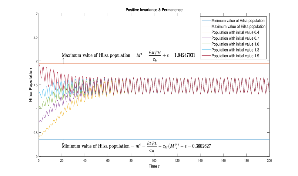
We can calculate Mε=ϱMφMcL+ε=1.94247931superscript𝑀𝜀subscriptitalic-ϱ𝑀subscript𝜑𝑀subscript𝑐𝐿𝜀1.94247931M^{\varepsilon}=\dfrac{\varrho_{M}\varphi_{M}}{c_{L}}+\varepsilon=1.94247931, mε=ϱLφL(cM)2(Mε)2cMε=0.3602627superscript𝑚𝜀subscriptitalic-ϱ𝐿subscript𝜑𝐿superscriptsubscript𝑐𝑀2superscriptsuperscript𝑀𝜀2subscript𝑐𝑀𝜀0.3602627m^{\varepsilon}=\dfrac{\varrho_{L}\varphi_{L}-(c_{M})^{2}(M^{\varepsilon})^{2}}{c_{M}}-\varepsilon=0.3602627 for ε=0.0001𝜀0.0001\varepsilon=0.0001. And ϱLφL=0.030329subscriptitalic-ϱ𝐿subscript𝜑𝐿0.030329\varrho_{L}\varphi_{L}=0.030329, (cM)2(Mε)2=0.0235487superscriptsubscript𝑐𝑀2superscriptsuperscript𝑀𝜀20.0235487(c_{M})^{2}(M^{\varepsilon})^{2}=0.0235487 which implies that ϱLφL>(cM)2(Mε)2subscriptitalic-ϱ𝐿subscript𝜑𝐿superscriptsubscript𝑐𝑀2superscriptsuperscript𝑀𝜀2\varrho_{L}\varphi_{L}>(c_{M})^{2}(M^{\varepsilon})^{2}. By taking ε=0𝜀0\varepsilon=0 we get M0=1.94237931superscript𝑀01.94237931M^{0}=1.94237931, m0=0.3603627superscript𝑚00.3603627m^{0}=0.3603627. Also, ϱLφL>(cM)2(M0)2subscriptitalic-ϱ𝐿subscript𝜑𝐿superscriptsubscript𝑐𝑀2superscriptsuperscript𝑀02\varrho_{L}\varphi_{L}>(c_{M})^{2}(M^{0})^{2}. From Theorem 2 we can say that system (1.2) is permanent, which is shown in Figure 2. Also, Kε={ϝ(t)R/mεϝ(t)Mε}subscript𝐾𝜀italic-ϝ𝑡𝑅superscript𝑚𝜀italic-ϝ𝑡superscript𝑀𝜀K_{\varepsilon}=\{\digamma(t)\in R/m^{\varepsilon}\leqslant\digamma(t)\leqslant M^{\varepsilon}\} = {ϝ(t)R/0.3602627ϝ(t)1.94247931}italic-ϝ𝑡𝑅0.3602627italic-ϝ𝑡1.94247931\{\digamma(t)\in R/0.3602627\leqslant\digamma(t)\leqslant 1.94247931\} and we just showed that ϱLφL>(cM)2(Mε)2subscriptitalic-ϱ𝐿subscript𝜑𝐿superscriptsubscript𝑐𝑀2superscriptsuperscript𝑀𝜀2\varrho_{L}\varphi_{L}>(c_{M})^{2}(M^{\varepsilon})^{2}. Therefore, from Theorem 1, Kεsubscript𝐾𝜀K_{\varepsilon} satisfies positive invariance property (w.r.t system (1.2)), which can also be seen in Figure 2.
Example 8.3. Let ϱ(t)=4.9+0.11(cos2t)italic-ϱ𝑡4.90.11superscript2𝑡\varrho(t)=4.9+0.11(\cos^{2}t), c(t)=6.40.025(sint)𝑐𝑡6.40.025𝑡c(t)=6.4-0.025(\sin t), φ(t)=0.02+0.01cost𝜑𝑡0.020.01𝑡\varphi(t)=0.02+0.01\cos t, q(t)=3.29𝑞𝑡3.29q(t)=3.29, E(t)=0.9𝐸𝑡0.9E(t)=0.9, ϑ1=2subscriptitalic-ϑ12\vartheta_{1}=2, ϑ2=1subscriptitalic-ϑ21\vartheta_{2}=1, then system (1.2) becomes
ϝ(t)=superscriptitalic-ϝ𝑡absent\digamma^{{}^{\prime}}(t)=

(4.9+0.11(cos2t))(0.02+0.01(cost))ϝ(t2)(0.02+0.01(cost))e2(0.02+0.01(cost))+(6.40.025(sint))(e2(0.02+0.01(cost))1)ϝ(t2)4.90.11superscript2𝑡0.020.01𝑡italic-ϝ𝑡20.020.01𝑡superscript𝑒20.020.01𝑡6.40.025𝑡superscript𝑒20.020.01𝑡1italic-ϝ𝑡2\dfrac{(4.9+0.11(\cos^{2}t))(0.02+0.01(\cos t))\digamma(t-2)}{(0.02+0.01(\cos t))e^{2(0.02+0.01(\cos t))}+(6.4-0.025(\sin t))(e^{2(0.02+0.01(\cos t))}-1)\digamma(t-2)}

(0.02+0.01(cost))ϝ(t)(6.40.025(sint))ϝ2(t)0.020.01𝑡italic-ϝ𝑡6.40.025𝑡superscriptitalic-ϝ2𝑡-(0.02+0.01(\cos t))\digamma(t)-(6.4-0.025(\sin t))\digamma^{2}(t)

(3.29)(0.9)(0.02+0.01(cost))ϝ(t1)(0.02+0.01(cost))e(0.02+0.01(cost)+(6.40.025(sint))(e0.02+0.01(cost)1)ϝ(t1)-\dfrac{(3.29)(0.9)(0.02+0.01(\cos t))\digamma(t-1)}{(0.02+0.01(\cos t))e^{(0.02+0.01(\cos t)}+(6.4-0.025(\sin t))(e^{0.02+0.01(\cos t)}-1)\digamma(t-1)}\cdot

For ε=0.0001𝜀0.0001\varepsilon=0.0001, we can compute ϱLφL=0.049subscriptitalic-ϱ𝐿subscript𝜑𝐿0.049\varrho_{L}\varphi_{L}=0.049, (cM)2(Mε)2=0.0231517superscriptsubscript𝑐𝑀2superscriptsuperscript𝑀𝜀20.0231517(c_{M})^{2}(M^{\varepsilon})^{2}=0.0231517 which implies that ϱLφL>(cM)2(Mε)2subscriptitalic-ϱ𝐿subscript𝜑𝐿superscriptsubscript𝑐𝑀2superscriptsuperscript𝑀𝜀2\varrho_{L}\varphi_{L}>(c_{M})^{2}(M^{\varepsilon})^{2}. Also from equation (5.1),

ϱ(t)φ2(t)eφ(t)ϑ1(φ(t)eφ(t)ϑ1+c(t)(eφ(t)ϑ11)Mε)2+4c(t)mε+2φ(t)+q(t)E(t)φ2(t)eφ(t)ϑ2(φ(t)eφ(t)ϑ2+c(t)(eφ(t)ϑ21)Mε)2italic-ϱ𝑡superscript𝜑2𝑡superscript𝑒𝜑𝑡subscriptitalic-ϑ1superscript𝜑𝑡superscript𝑒𝜑𝑡subscriptitalic-ϑ1𝑐𝑡superscript𝑒𝜑𝑡subscriptitalic-ϑ11superscript𝑀𝜀24𝑐𝑡superscript𝑚𝜀2𝜑𝑡𝑞𝑡𝐸𝑡superscript𝜑2𝑡superscript𝑒𝜑𝑡subscriptitalic-ϑ2superscript𝜑𝑡superscript𝑒𝜑𝑡subscriptitalic-ϑ2𝑐𝑡superscript𝑒𝜑𝑡subscriptitalic-ϑ21superscript𝑀𝜀2\dfrac{-\varrho(t)\varphi^{2}(t)e^{\varphi(t)\vartheta_{1}}}{(\varphi(t)e^{\varphi(t)\vartheta_{1}}+c(t)(e^{\varphi(t)\vartheta_{1}}-1)M^{\varepsilon})^{2}}+4c(t)m^{\varepsilon}+2\varphi(t)+\dfrac{q(t)E(t)\varphi^{2}(t)e^{\varphi(t)\vartheta_{2}}}{(\varphi(t)e^{\varphi(t)\vartheta_{2}}+c(t)(e^{\varphi(t)\vartheta_{2}}-1)M^{\varepsilon})^{2}}

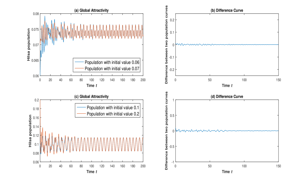
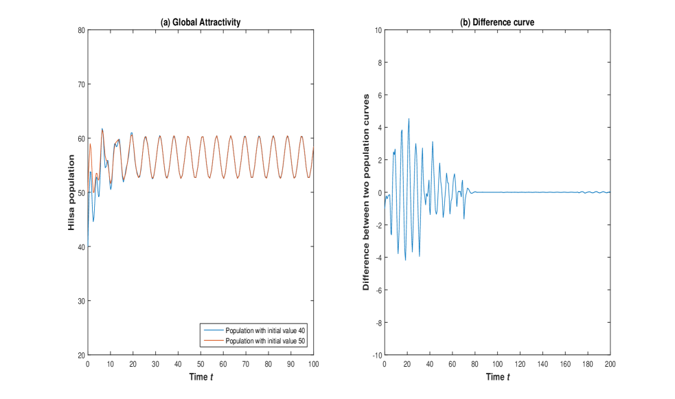
=0.063903198>0absent0.0639031980=0.063903198>0. Hence from Theorem 3, ϝ(t)superscriptitalic-ϝ𝑡\digamma^{\ast}(t), a bounded (enclosed within positive values) and positive (>0absent0>0) solution to system (1.2) is globally attractive, as seen in Figure 3(a). The difference between the two trajectories starting at initial values ϝ(t0)=0.06italic-ϝsubscript𝑡00.06\digamma(t_{0})=0.06 and ϝ(t0)=0.07italic-ϝsubscript𝑡00.07\digamma(t_{0})=0.07 is plotted against time t𝑡t in Figure 3(b). It is now clear that as t𝑡t\to\infty the difference between the two trajectories tends to zero.
Example 8.4. Let ϱ(t)=8(sint)italic-ϱ𝑡8𝑡\varrho(t)=8-(\sin t), c(t)=7+(cost)𝑐𝑡7𝑡c(t)=7+(\cos t), φ=0.023𝜑0.023\varphi=0.023, q(t)=0.48𝑞𝑡0.48q(t)=0.48, E(t)=9𝐸𝑡9E(t)=9, ϑ1=2subscriptitalic-ϑ12\vartheta_{1}=2, ϑ2=1subscriptitalic-ϑ21\vartheta_{2}=1, then system (1.2) becomes

ϝ(t)=(8(sint))(0.023)ϝ(t2)(0.023)e2(0.023)+(7+(cost))(e2(0.023)1)ϝ(t2)superscriptitalic-ϝ𝑡8𝑡0.023italic-ϝ𝑡20.023superscript𝑒20.0237𝑡superscript𝑒20.0231italic-ϝ𝑡2\digamma^{{}^{\prime}}(t)=\dfrac{(8-(\sin t))(0.023)\digamma(t-2)}{(0.023)e^{2(0.023)}+(7+(\cos t))(e^{2(0.023)}-1)\digamma(t-2)}

(0.023)ϝ(t)(7+cost))ϝ2(t)-(0.023)\digamma(t)-(7+\cos t))\digamma^{2}(t) (0.48)(9)(0.023)ϝ(t1)(0.023)e0.023+(7+(cost))(e0.0231)ϝ(t1)-\dfrac{(0.48)(9)(0.023)\digamma(t-1)}{(0.023)e^{0.023}+(7+(\cos t))(e^{0.023}-1)\digamma(t-1)}\cdot

By simple numerical computation, we have ϱLφL=0.161subscriptitalic-ϱ𝐿subscript𝜑𝐿0.161\varrho_{L}\varphi_{L}=0.161, (cM)2(Mε)2=0.07661824superscriptsubscript𝑐𝑀2superscriptsuperscript𝑀𝜀20.07661824(c_{M})^{2}(M^{\varepsilon})^{2}=0.07661824 for ε=0.0001𝜀0.0001\varepsilon=0.0001. This implies that ϱLφL>(cM)2(Mε)2subscriptitalic-ϱ𝐿subscript𝜑𝐿superscriptsubscript𝑐𝑀2superscriptsuperscript𝑀𝜀2\varrho_{L}\varphi_{L}>(c_{M})^{2}(M^{\varepsilon})^{2}. Also from equation (5.1),

ϱ(t)φ2(t)eφ(t)ϑ1(φ(t)eφ(t)ϑ1+c(t)(eφ(t)ϑ11)Mε)2+4c(t)mε+2φ(t)+q(t)E(t)φ2(t)eφ(t)ϑ2(φ(t)eφ(t)ϑ2+c(t)(eφ(t)ϑ21)Mε)2italic-ϱ𝑡superscript𝜑2𝑡superscript𝑒𝜑𝑡subscriptitalic-ϑ1superscript𝜑𝑡superscript𝑒𝜑𝑡subscriptitalic-ϑ1𝑐𝑡superscript𝑒𝜑𝑡subscriptitalic-ϑ11superscript𝑀𝜀24𝑐𝑡superscript𝑚𝜀2𝜑𝑡𝑞𝑡𝐸𝑡superscript𝜑2𝑡superscript𝑒𝜑𝑡subscriptitalic-ϑ2superscript𝜑𝑡superscript𝑒𝜑𝑡subscriptitalic-ϑ2𝑐𝑡superscript𝑒𝜑𝑡subscriptitalic-ϑ21superscript𝑀𝜀2\dfrac{-\varrho(t)\varphi^{2}(t)e^{\varphi(t)\vartheta_{1}}}{(\varphi(t)e^{\varphi(t)\vartheta_{1}}+c(t)(e^{\varphi(t)\vartheta_{1}}-1)M^{\varepsilon})^{2}}+4c(t)m^{\varepsilon}+2\varphi(t)+\dfrac{q(t)E(t)\varphi^{2}(t)e^{\varphi(t)\vartheta_{2}}}{(\varphi(t)e^{\varphi(t)\vartheta_{2}}+c(t)(e^{\varphi(t)\vartheta_{2}}-1)M^{\varepsilon})^{2}}

=0.08561413>0absent0.085614130=0.08561413>0. Hence from Theorem 3, ϝ(t)superscriptitalic-ϝ𝑡\digamma^{\ast}(t), a bounded (enclosed within positive values) and positive (>0absent0>0) solution to system (1.2) is globally attractive, as shown in Figure 3(c). The difference between the two trajectories starting at initial values ϝ(t0)=0.1italic-ϝsubscript𝑡00.1\digamma(t_{0})=0.1 and ϝ(t0)=0.2italic-ϝsubscript𝑡00.2\digamma(t_{0})=0.2 is plotted against time t𝑡t in Figure 3(d). It is now clear that as t𝑡t\to\infty the difference between the two trajectories tends to zero.
Example 8.5. Let ϱ(t)=1.3+0.33sintitalic-ϱ𝑡1.30.33𝑡\varrho(t)=1.3+0.33\sin t, c(t)=0.20.1428cost𝑐𝑡0.20.1428𝑡c(t)=0.2-0.1428\cos t, φ=0.02+0.01cost𝜑0.020.01𝑡\varphi=0.02+0.01\cos t, q(t)=0.0250.0166sint𝑞𝑡0.0250.0166𝑡q(t)=0.025-0.0166\sin t, E(t)=10.5cos2t𝐸𝑡10.5superscript2𝑡E(t)=1-0.5\cos^{2}t, ϑ1=2subscriptitalic-ϑ12\vartheta_{1}=2, ϑ2=1subscriptitalic-ϑ21\vartheta_{2}=1 and choose Θ=2πΘ2𝜋\Theta=2\pi then system (1.2) becomes
ϝ(t)=superscriptitalic-ϝ𝑡absent\digamma^{{}^{\prime}}(t)=

(1.3+0.33sint)(0.02+0.01cost)ϝ(t2)(0.02+0.01cost)e2(0.02+0.01cost)+(0.20.1428cost)(e2(0.02+0.01cost)1)ϝ(t2)1.30.33𝑡0.020.01𝑡italic-ϝ𝑡20.020.01𝑡superscript𝑒20.020.01𝑡0.20.1428𝑡superscript𝑒20.020.01𝑡1italic-ϝ𝑡2\dfrac{(1.3+0.33\sin t)(0.02+0.01\cos t)\digamma(t-2)}{(0.02+0.01\cos t)e^{2(0.02+0.01\cos t)}+(0.2-0.1428\cos t)(e^{2(0.02+0.01\cos t)}-1)\digamma(t-2)}

(0.02+0.01(cost))ϝ(t)(0.20.1428cost))ϝ2(t)-(0.02+0.01(\cos t))\digamma(t)-(0.2-0.1428\cos t))\digamma^{2}(t)

(0.0250.0166sint)(10.5cos2t))(0.02+0.01cost)ϝ(t1)(0.02+0.01cost)e0.02+0.01cost+(0.20.1428cost)(e0.02+0.01cost1)ϝ(t1)-\dfrac{(0.025-0.0166\sin t)(1-0.5\cos^{2}t))(0.02+0.01\cos t)\digamma(t-1)}{(0.02+0.01\cos t)e^{0.02+0.01\cos t}+(0.2-0.1428\cos t)(e^{0.02+0.01\cos t}-1)\digamma(t-1)}\cdot

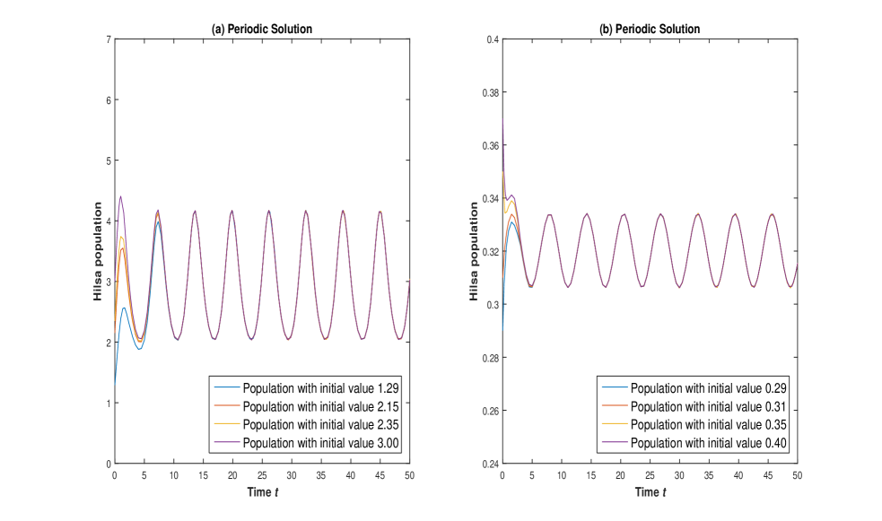
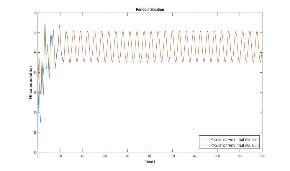
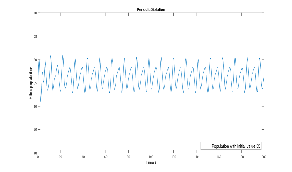
For ε=0.0001𝜀0.0001\varepsilon=0.0001, we can compute ϱφ~=0.013~italic-ϱ𝜑0.013\tilde{\varrho\varphi}=0.013, (c~Mε)2=0.00081812superscript~𝑐superscript𝑀𝜀20.00081812(\tilde{c}M^{\varepsilon})^{2}=0.00081812 which implies that ϱφ~>(c~Mε)2.~italic-ϱ𝜑superscript~𝑐superscript𝑀𝜀2\tilde{\varrho\varphi}>(\tilde{c}M^{\varepsilon})^{2}. Hence from Theorem 5, system (1.2) possesses not less than one positive(>0absent0>0) ΘΘ\Theta-periodic solution, which is also shown in Figure 4(a).
Example 8.6. Let ϱ(t)=7+0.33costitalic-ϱ𝑡70.33𝑡\varrho(t)=7+0.33\cos t, c(t)=50.25sint𝑐𝑡50.25𝑡c(t)=5-0.25\sin t, φ=0.02+0.01cost𝜑0.020.01𝑡\varphi=0.02+0.01\cos t, q(t)=0.0250.0166sint𝑞𝑡0.0250.0166𝑡q(t)=0.025-0.0166\sin t, E(t)=10.5cos2t𝐸𝑡10.5superscript2𝑡E(t)=1-0.5\cos^{2}t, ϑ1=2subscriptitalic-ϑ12\vartheta_{1}=2, ϑ2=1subscriptitalic-ϑ21\vartheta_{2}=1 and choose Θ=2πΘ2𝜋\Theta=2\pi then system (1.2) becomes
ϝ(t)=superscriptitalic-ϝ𝑡absent\digamma^{{}^{\prime}}(t)=

(7+0.33cost)(0.02+0.01cost)ϝ(t2)(0.02+0.01cost)e2(0.02+0.01cost)+(50.25sint)(e2(0.02+0.01cost))1)ϝ(t2)\dfrac{(7+0.33\cos t)(0.02+0.01\cos t)\digamma(t-2)}{(0.02+0.01\cos t)e^{2(0.02+0.01\cos t)}+(5-0.25\sin t)(e^{2(0.02+0.01\cos t)})-1)\digamma(t-2)}

(0.02+0.01cost)ϝ(t)(50.25sint)ϝ2(t)0.020.01𝑡italic-ϝ𝑡50.25𝑡superscriptitalic-ϝ2𝑡-(0.02+0.01\cos t)\digamma(t)-(5-0.25\sin t)\digamma^{2}(t)

(0.0250.0166sint)(10.5cos2t))(0.02+0.01cost))ϝ(t1)(0.02+0.01cost)e0.02+0.01cost+(50.25sint)(e0.02+0.01cost1)ϝ(t1)-\dfrac{(0.025-0.0166\sin t)(1-0.5\cos^{2}t))(0.02+0.01\cos t))\digamma(t-1)}{(0.02+0.01\cos t)e^{0.02+0.01\cos t}+(5-0.25\sin t)(e^{0.02+0.01\cos t}-1)\digamma(t-1)}\cdot

By simple numerical computation, ϱφ~=0.07~italic-ϱ𝜑0.07\tilde{\varrho\varphi}=0.07, (c~Mε)2=0.0514719superscript~𝑐superscript𝑀𝜀20.0514719(\tilde{c}M^{\varepsilon})^{2}=0.0514719 for ε=0.0001𝜀0.0001\varepsilon=0.0001. This implies that ϱφ~>(c~Mε)2.~italic-ϱ𝜑superscript~𝑐superscript𝑀𝜀2\tilde{\varrho\varphi}>(\tilde{c}M^{\varepsilon})^{2}. Hence we have, from Theorem 5, system (1.2) possesses minimum one positive(>0absent0>0) ΘΘ\Theta-periodic solution, as shown in Figure 4(b).
Example 8.7. Let ϱ(t)=14+0.1cos2titalic-ϱ𝑡140.1superscript2𝑡\varrho(t)=14+0.1\cos^{2}t, c(t)=2+0.33sint𝑐𝑡20.33𝑡c(t)=2+0.33\sin t, φ=0.032𝜑0.032\varphi=0.032, q(t)=0.030.01sint𝑞𝑡0.030.01𝑡q(t)=0.03-0.01\sin t, E(t)=235𝐸𝑡235E(t)=235, ϑ1=2subscriptitalic-ϑ12\vartheta_{1}=2, ϑ2=1subscriptitalic-ϑ21\vartheta_{2}=1 and choose Θ=2πΘ2𝜋\Theta=2\pi then system (1.2) becomes

ϝ(t)=superscriptitalic-ϝ𝑡absent\digamma^{{}^{\prime}}(t)= (14+0.1cos2t)(0.032)ϝ(t2)(0.032)e2(0.032)+(2+0.33sint)(e2(0.032))1)ϝ(t2)\dfrac{(14+0.1\cos^{2}t)(0.032)\digamma(t-2)}{(0.032)e^{2(0.032)}+(2+0.33\sin t)(e^{2(0.032)})-1)\digamma(t-2)}

(0.032)ϝ(t)(2+0.33sint)ϝ2(t)0.032italic-ϝ𝑡20.33𝑡superscriptitalic-ϝ2𝑡-(0.032)\digamma(t)-(2+0.33\sin t)\digamma^{2}(t) (0.030.01sint)(235)(0.032)ϝ(t1)(0.032)e0.032+(2+0.33sint)(e0.0321)ϝ(t1)-\dfrac{(0.03-0.01\sin t)(235)(0.032)\digamma(t-1)}{(0.032)e^{0.032}+(2+0.33\sin t)(e^{0.032}-1)\digamma(t-1)}\cdot

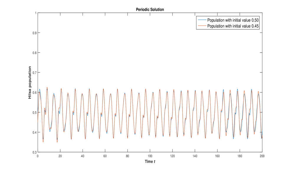
We can calculate ϱφ~=0.4496~italic-ϱ𝜑0.4496\tilde{\varrho\varphi}=0.4496, (c~Mε)2=0.2915307superscript~𝑐superscript𝑀𝜀20.2915307(\tilde{c}M^{\varepsilon})^{2}=0.2915307 for ε=0.0001𝜀0.0001\varepsilon=0.0001. This implies that ϱφ~>(c~Mε)2.~italic-ϱ𝜑superscript~𝑐superscript𝑀𝜀2\tilde{\varrho\varphi}>(\tilde{c}M^{\varepsilon})^{2}. Hence from Theorem 5, system (1.2) has one or more positive(>0absent0>0) ΘΘ\Theta-periodic solutions. From Figure 5 we can observe that system (1.2) admits triple-periodic solution. Also, a double periodic solution can be seen in Figure 2.
Example 8.8. Let ϱ(t)=6+cos(t)8italic-ϱ𝑡6𝑡8\varrho(t)=6+\dfrac{\cos(t)}{8}, c(t)=0.01+0.0011cost𝑐𝑡0.010.0011𝑡c(t)=0.01+0.0011\cos t, φ(t)=0.1𝜑𝑡0.1\varphi(t)=0.1, q(t)=0.3𝑞𝑡0.3q(t)=0.3,
E(t)=10𝐸𝑡10E(t)=10, ϑ1=2subscriptitalic-ϑ12\vartheta_{1}=2, ϑ2=1subscriptitalic-ϑ21\vartheta_{2}=1 and choose Θ=2πΘ2𝜋\Theta=2\pi then system (1.2) becomes
ϝ(t)=superscriptitalic-ϝ𝑡absent\digamma^{{}^{\prime}}(t)=

(6+cost8)(0.1)ϝ(t2)(0.1)e2(0.1)+(0.01+0.0011cost)(e2(0.1)1)ϝ(t2)6𝑡80.1italic-ϝ𝑡20.1superscript𝑒20.10.010.0011𝑡superscript𝑒20.11italic-ϝ𝑡2\dfrac{(6+\dfrac{\cos t}{8})(0.1)\digamma(t-2)}{(0.1)e^{2(0.1)}+(0.01+0.0011\cos t)(e^{2(0.1)}-1)\digamma(t-2)} (0.1)ϝ(t)0.1italic-ϝ𝑡-(0.1)\digamma(t)

(0.01+0.0011cost)ϝ2(t)0.010.0011𝑡superscriptitalic-ϝ2𝑡-(0.01+0.0011\cos t)\digamma^{2}(t) (0.3)(10)(0.1)ϝ(t1)(0.1)e0.1+(0.01+0.0011cost)(e0.11)ϝ(t1)-\dfrac{(0.3)(10)(0.1)\digamma(t-1)}{(0.1)e^{0.1}+(0.01+0.0011\cos t)(e^{0.1}-1)\digamma(t-1)}\cdot

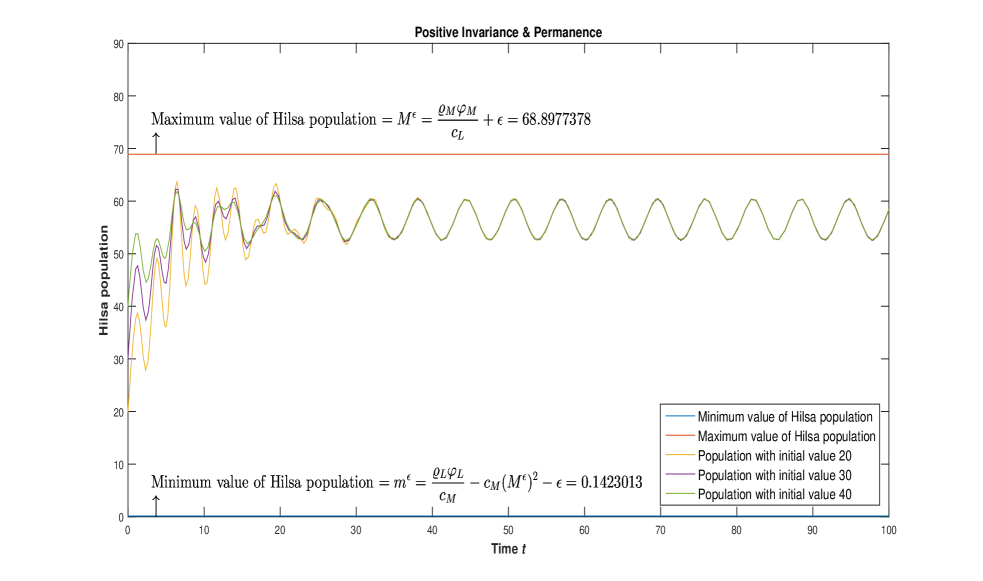
We can calculate Mε=ϱMφMcL+ε=68.8977378superscript𝑀𝜀subscriptitalic-ϱ𝑀subscript𝜑𝑀subscript𝑐𝐿𝜀68.8977378M^{\varepsilon}=\dfrac{\varrho_{M}\varphi_{M}}{c_{L}}+\varepsilon=68.8977378, mε=ϱLφL(cM)2(Mε)2cMε=0.1423013superscript𝑚𝜀subscriptitalic-ϱ𝐿subscript𝜑𝐿superscriptsubscript𝑐𝑀2superscriptsuperscript𝑀𝜀2subscript𝑐𝑀𝜀0.1423013m^{\varepsilon}=\dfrac{\varrho_{L}\varphi_{L}-(c_{M})^{2}(M^{\varepsilon})^{2}}{c_{M}}-\varepsilon=0.1423013 for ε=0.0001𝜀0.0001\varepsilon=0.0001. And ϱLφL=0.5875subscriptitalic-ϱ𝐿subscript𝜑𝐿0.5875\varrho_{L}\varphi_{L}=0.5875, (cM)2(Mε)2=0.584865337superscriptsubscript𝑐𝑀2superscriptsuperscript𝑀𝜀20.584865337(c_{M})^{2}(M^{\varepsilon})^{2}=0.584865337 which implies that ϱLφL>(cM)2(Mε)2subscriptitalic-ϱ𝐿subscript𝜑𝐿superscriptsubscript𝑐𝑀2superscriptsuperscript𝑀𝜀2\varrho_{L}\varphi_{L}>(c_{M})^{2}(M^{\varepsilon})^{2}. By taking ε=0𝜀0\varepsilon=0, we get M0=68.8976378superscript𝑀068.8976378M^{0}=68.8976378, m0=0.1424013superscript𝑚00.1424013m^{0}=0.1424013. Also, ϱLφL>(cM)2(M0)2subscriptitalic-ϱ𝐿subscript𝜑𝐿superscriptsubscript𝑐𝑀2superscriptsuperscript𝑀02\varrho_{L}\varphi_{L}>(c_{M})^{2}(M^{0})^{2}. From Theorem 2, system (1.2) is permanent, which is shown in Figure 6.
Also, Kε={ϝ(t)R/mεϝ(t)Mε}subscript𝐾𝜀italic-ϝ𝑡𝑅superscript𝑚𝜀italic-ϝ𝑡superscript𝑀𝜀K_{\varepsilon}=\{\digamma(t)\in R/m^{\varepsilon}\leqslant\digamma(t)\leqslant M^{\varepsilon}\} = {ϝ(t)R/0.1423013ϝ(t)68.8977378}italic-ϝ𝑡𝑅0.1423013italic-ϝ𝑡68.8977378\{\digamma(t)\in R/0.1423013\leqslant\digamma(t)\leqslant 68.8977378\}
and we just showed that ϱLφL>(cM)2(Mε)2subscriptitalic-ϱ𝐿subscript𝜑𝐿superscriptsubscript𝑐𝑀2superscriptsuperscript𝑀𝜀2\varrho_{L}\varphi_{L}>(c_{M})^{2}(M^{\varepsilon})^{2}. Therefore, from Theorem 1, Kεsubscript𝐾𝜀K_{\varepsilon} satisfies the property of positive invariance (w.r.t system (1.2)), which can also be seen in Figure 6.
Also from equation (5.1),

ϱ(t)φ2(t)eφ(t)ϑ1(φ(t)eφ(t)ϑ1+c(t)(eφ(t)ϑ11)Mε)2+4c(t)mε+2φ(t)+q(t)E(t)φ2(t)eφ(t)ϑ2(φ(t)eφ(t)ϑ2+c(t)(eφ(t)ϑ21)Mε)2italic-ϱ𝑡superscript𝜑2𝑡superscript𝑒𝜑𝑡subscriptitalic-ϑ1superscript𝜑𝑡superscript𝑒𝜑𝑡subscriptitalic-ϑ1𝑐𝑡superscript𝑒𝜑𝑡subscriptitalic-ϑ11superscript𝑀𝜀24𝑐𝑡superscript𝑚𝜀2𝜑𝑡𝑞𝑡𝐸𝑡superscript𝜑2𝑡superscript𝑒𝜑𝑡subscriptitalic-ϑ2superscript𝜑𝑡superscript𝑒𝜑𝑡subscriptitalic-ϑ2𝑐𝑡superscript𝑒𝜑𝑡subscriptitalic-ϑ21superscript𝑀𝜀2\dfrac{-\varrho(t)\varphi^{2}(t)e^{\varphi(t)\vartheta_{1}}}{(\varphi(t)e^{\varphi(t)\vartheta_{1}}+c(t)(e^{\varphi(t)\vartheta_{1}}-1)M^{\varepsilon})^{2}}+4c(t)m^{\varepsilon}+2\varphi(t)+\dfrac{q(t)E(t)\varphi^{2}(t)e^{\varphi(t)\vartheta_{2}}}{(\varphi(t)e^{\varphi(t)\vartheta_{2}}+c(t)(e^{\varphi(t)\vartheta_{2}}-1)M^{\varepsilon})^{2}}

=0.269876035>0absent0.2698760350=0.269876035>0. Hence from Theorem 3, ϝ(t)superscriptitalic-ϝ𝑡\digamma^{\ast}(t), bounded (bordered by positive values) positive (>0absent0>0) solution to system (1.2) is globally attractive, as seen in Figure 7(a). The difference between two trajectories starting with initial values ϝ(t0)=40italic-ϝsubscript𝑡040\digamma(t_{0})=40 and ϝ(t0)=50italic-ϝsubscript𝑡050\digamma(t_{0})=50 is plotted over time t𝑡t in Figure 7(b). It is clear that as t𝑡t\to\infty the difference between these trajectories tends to zero.

And ϱφ~=0.6~italic-ϱ𝜑0.6\tilde{\varrho\varphi}=0.6, (c~Mε)2=0.474689827superscript~𝑐superscript𝑀𝜀20.474689827(\tilde{c}M^{\varepsilon})^{2}=0.474689827 which implies that ϱφ~>(c~Mε)2~italic-ϱ𝜑superscript~𝑐superscript𝑀𝜀2\tilde{\varrho\varphi}>(\tilde{c}M^{\varepsilon})^{2}. Hence using Theorem 5, there is minimum one positive(>0absent0>0) ΘΘ\Theta-periodic solution to system (1.2) as shown in Figure 8. A double periodic solution can be noticed in Figure 9.

On the other hand, let ϱ(t)=6+cos((10π/3)t)8italic-ϱ𝑡610𝜋3𝑡8\varrho(t)=6+\frac{\cos((10\pi/\sqrt{3})t)}{8}, i.e, period is rationally independent. According to theorem 6, there is an almost periodic solution as shown in Figure 10.
Example 8.9. Let ϱ(t)=6+cos(t)8italic-ϱ𝑡6𝑐𝑜𝑠𝑡8\varrho(t)=6+\frac{cos(t)}{8}, φ(t)=0.10𝜑𝑡0.10\varphi(t)=0.10, c(t)=0.01(0.0011)cos(t)𝑐𝑡0.010.0011𝑐𝑜𝑠𝑡c(t)=0.01-(0.0011)cos(t), q(t)=0.3𝑞𝑡0.3q(t)=0.3, E(t)=10𝐸𝑡10E(t)=10. We plot the population curves for different values of ϑ1subscriptitalic-ϑ1\vartheta_{1} and ϑ2subscriptitalic-ϑ2\vartheta_{2} in figures 11 and 12. Our observations are shown in Tables 1 and 2.
Example 8.10. Let ϱ(t)=1.3italic-ϱ𝑡1.3\varrho(t)=1.3, φ(t)=0.02+(0.01)cos(t)𝜑𝑡0.020.01𝑐𝑜𝑠𝑡\varphi(t)=0.02+(0.01)cos(t), c(t)=0.005𝑐𝑡0.005c(t)=0.005, q(t)=0.9𝑞𝑡0.9q(t)=0.9, E(t)=1.3𝐸𝑡1.3E(t)=1.3. The population curves for different values of ϑ1subscriptitalic-ϑ1\vartheta_{1} and ϑ2subscriptitalic-ϑ2\vartheta_{2} are shown in figures 13 and 14. Our observations are shown in Tables 3 and 4.

9 Conclusion

The dynamical characteristics of any real-world ecological model depend explicitly on time. Most of the environmental factors vary with time and thus incorporating temporal inhomogeneity into an ecological model helps to understand it better.

The present work is essentially concerned with the age-based growth model of hilsa fish with time-variant parameters. We have obtained the sufficient condition for positive invariance from Theorem 1 and the sufficient condition for permanence from Theorem 2, respectively. Also, if ε=0𝜀0\varepsilon=0 in Theorem 1, we obtain the condition in Theorem 2. This means that if Kεsubscript𝐾𝜀K_{\varepsilon} is positively invariant in system (1.2), then system (1.2) must be permanent, which is pretty clear from figures 1, 2 and 6. That is, if the population of hilsa lies within a particular range (given by [mε,Mε]superscript𝑚𝜀superscript𝑀𝜀[m^{\varepsilon},M^{\varepsilon}] (see Theorem 1)) and lasts forever (as t𝑡t\rightarrow\infty) in that particular range then the population would never go extinct. In addition, we attain suitable conditions for global attractivity of a bounded positive solution by formulating a scalar function, namely the Lyapunov function in Theorem 3. In figures3(a) and (c) and 7(a), there is one such trajectory (hilsa population) in each of these figures that attracts the other trajectory (hilsa population starting at a different initial value) towards it, proving the global stability of hilsa population.

It is known that birth, growth, spawning and, immigration of hilsa is very much seasonal, thus indicating that the environmental factors that influence the life cycle of hilsa are seasonal. Taking this into account, in Theorems 4 and 5, with the help of Brouwer fixed point and continuation theorems we have obtained some constraints for a positive periodic solution of system (1.2). We can see that if ε𝜀\varepsilon is chosen suitably and condition in Theorem 1 holds, then the condition in Theorem 5 holds, that is, Theorem 5 is weaker than Theorem 1. Finally, in Theorem 6 we have proved that there is only one solution to system (1.2) which is almost periodic in nature that is distinct from every other solution. Figures 4, 5, 8 and 9 show that hilsa population follows a periodic cycle and figure 10 shows that hilsa population can also be quasi-periodic. This means that the fluctuations in the hilsa population follow a regular repeating pattern. For example, in Figure 4 we see that the changes in hilsa population that includes changes due to various factors like birth, death, food resources, fishing, etc, repeat every five years. This before hand prediction helps in taking precautionary measures to prevent a fall in the hilsa population.

Hilsa stocks have been fast decreasing in the river systems. Thus conserving the population of hilsa and maintaining its global stability is one of the major concerns of ecologists across India and Bangladesh. The role played by ϑ1subscriptitalic-ϑ1\vartheta_{1} and ϑ2subscriptitalic-ϑ2\vartheta_{2} (delay in maturity and delay in harvest respectively) in shaping the dynamical aspects of the system (1.2) of hilsa is as shown in Tables 1, 2, 3 and 4. In Table 1, we see that when the delay in maturity ϑ1subscriptitalic-ϑ1\vartheta_{1} increases to 2.208 (critical value of ϑ1subscriptitalic-ϑ1\vartheta_{1}) with ϑ2subscriptitalic-ϑ2\vartheta_{2} remaining constant at 1, there is a drastic change in the dynamical characteristics of the system. Then if ϑ2subscriptitalic-ϑ2\vartheta_{2} increases beyond 1, the system regains its dynamical characteristics. This means that for a maturity delay of 2.208, the delay in harvest must be greater than 1. Similarly, from Table 3, for a maturity delay of 2.24, the delay in harvest must be greater than 1 (see Figures 11, 12, 13 and 14). This interplay between ϑ1subscriptitalic-ϑ1\vartheta_{1} and ϑ2subscriptitalic-ϑ2\vartheta_{2} plays a significant role in shaping the dynamical characteristics of the system (1.2). Therefore, a change in the fishing pattern, by paying extra attention to immature hilsa and taking into account the size and body weight of hilsa before harvesting, and a change in the approach towards the ecological model of hilsa, by acknowledging the importance of time-variant parameters, can stop hilsa from becoming extinct.

Appendix A

The rate at which the population changes depends on the following aspects: birth rate, rate of death and intraspecific competitiveness (either crowding or head-on intervention). Death rate and intraspecific competition rate both together contribute to the decline rate, which is instantaneous. Considering this we revise the standard logistic ordinary differential equation [1] into:

dϝ(t)dt=ϱϝ(t)φϝ(t)cϝ2(t),𝑑italic-ϝ𝑡𝑑𝑡italic-ϱitalic-ϝ𝑡𝜑italic-ϝ𝑡𝑐superscriptitalic-ϝ2𝑡\frac{d\digamma(t)}{dt}=\varrho\digamma(t)-\varphi\digamma(t)-c\digamma^{2}(t), (A1)𝐴1

where ϱitalic-ϱ\varrho, φ𝜑\varphi and c𝑐c denote the birth, death and removal (due to intraspecific competition) coefficients respectively for ϝ(t)italic-ϝ𝑡\digamma(t). If r=ϱφ𝑟italic-ϱ𝜑r=\varrho-\varphi (i.e. intrinsic growth rate of ϝ(t)italic-ϝ𝑡\digamma(t)) and K=ϱφc𝐾italic-ϱ𝜑𝑐K=\frac{\varrho-\varphi}{c} (i.e. environmental carrying capacity of ϝ(t)italic-ϝ𝑡\digamma(t)), then Eq. (A1)𝐴1(A1) becomes the classical logistic equation:

dϝ(t)dt=rϝ(t)(1ϝ(t)K).𝑑italic-ϝ𝑡𝑑𝑡𝑟italic-ϝ𝑡1italic-ϝ𝑡𝐾\frac{d\digamma(t)}{dt}=r\digamma(t)\bigg{(}1-\frac{\digamma(t)}{K}\bigg{)}. (A2)𝐴2

In (A1)𝐴1(A1), the rate of decline and rate of growth (both of which depend on the density of population at the current instant t𝑡t) are denoted by {φϝ(t)+cϝ2(t)}𝜑italic-ϝ𝑡𝑐superscriptitalic-ϝ2𝑡\{\varphi\digamma(t)+c\digamma^{2}(t)\} and ϱϝ(t)italic-ϱitalic-ϝ𝑡\varrho\digamma(t) respectively. In order to acquire an equation to describe the number of individuals that are alive at tϑ𝑡italic-ϑt-\vartheta shall be still alive at t𝑡t, consider a first ordered ODE of ϝ(t)italic-ϝ𝑡\digamma(t) as a function of ϝ(tϑ)italic-ϝ𝑡italic-ϑ\digamma(t-\vartheta) and solve it as follows:

dϝ(t)dt=φϝ(t)cϝ2(t).𝑑italic-ϝ𝑡𝑑𝑡𝜑italic-ϝ𝑡𝑐superscriptitalic-ϝ2𝑡\begin{array}[]{l}\dfrac{d\digamma(t)}{dt}=-\varphi\digamma(t)-c\digamma^{2}(t).\end{array}

Using variable separable technique and then integrating from tϑ𝑡italic-ϑt-\vartheta to t𝑡t, we get

ϝ(tϑ)ϝ(t)1φϝ(t)+cϝ2(t)𝑑ϝ=tϑt𝑑t,superscriptsubscriptitalic-ϝ𝑡italic-ϑitalic-ϝ𝑡1𝜑italic-ϝ𝑡𝑐superscriptitalic-ϝ2𝑡differential-ditalic-ϝsuperscriptsubscript𝑡italic-ϑ𝑡differential-d𝑡\begin{array}[]{l}\int_{\digamma(t-\vartheta)}^{\digamma(t)}\frac{1}{\varphi\digamma(t)+c\digamma^{2}(t)}d\digamma=-\int_{t-\vartheta}^{t}dt,\end{array}

and hence

ϝ(t)=φϝ(tϑ)φeφϑ+c(eφϑ1)ϝ(tϑ).italic-ϝ𝑡𝜑italic-ϝ𝑡italic-ϑ𝜑superscript𝑒𝜑italic-ϑ𝑐superscript𝑒𝜑italic-ϑ1italic-ϝ𝑡italic-ϑ\digamma(t)=\frac{\varphi\digamma(t-\vartheta)}{\varphi e^{\varphi\vartheta}+c(e^{\varphi\vartheta}-1)\digamma(t-\vartheta)}. (A3)𝐴3

References

  • [1] J. Arino, L. Wang, and G. S. K. Wolkowicz, An alternative formulation for a delayed logistic equation, J. Theor. Biol., 241(1) (2006), 109-119.
  • [2] D. Auslander, G. F. Oster, and C. Huffaker, Dynamics of interacting populations, J. Franklin Inst., 297(5) (1974), 345-375.
  • [3] R. G. Bartle and R. G. Bartle, The elements of real analysis, Wiley, New York (1964).
  • [4] J. R. Beddington and R. M. May, Time delays are not necessarily destabilizing, Math. Biosci., 27(1-2) (1975), 109-117.
  • [5] U. Bhaumik and A. P. Sharma, The fishery of Indian Shad (Tenualosa ilisha) in the Bhagirathi-Hooghly river system, Fish. Chimes, 31(8) (2011), 21-27.
  • [6] U. Bhaumik, Review of global studies on food, growth and maturity profile of Indian Shad (Tenualosa ilisha), Int. J. Curr. Res. Acad. Rev., 3(10) (2015), 127-139.
  • [7] S. P. Blythe, R. M. Nisbet, and W. S. C. Gurney, Instability and complex dynamic behavior in population models with long time delays, Theor. Popul. Biol., 22(2) (1982), 147-176.
  • [8] J. B. Barbara, Age related changes in photosynthesis of woody plants, Trends Plant Sci., 5(8) (2000), 349-353.
  • [9] L. E. J. Brouwer, Uber abbildung von mannigfaltigkeiten, Math. Ann., 71 (1911), 97-115.
  • [10] F. Chen, Y. Chen, and J. Shi, Stability of the boundary solution of a nonautonomous predator-prey system with the Beddington-DeAngelis functional response, J. Math. Anal. Appl., 344(2) (2008), 1057-1067.
  • [11] J. Cui and Y. Takeuchi, Permanence, extinction and periodic solution of predator-prey system with Beddington-DeAngelis functional response, J. Math. Anal. Appl., 317(2) (2006), 464-474.
  • [12] W. J. Cunningham, A nonlinear differential-difference equation of growth, Proc. Natl. Acad. Sci. USA, 40(8) (1954), 708-713.
  • [13] Department of Fisheries, Hilsa fishery management, Government of Bangladesh, Dhaka (2013).
  • [14] R. W. Eschmeyer, D. E. Manges, and O. I. Haslbauer, Spring fishing on several T.V.A. storage reservoirs, J. Tenn. Acad. Sci., 21(1) (1946), 78-88.
  • [15] M. Fan and Y. Kuang, Dynamics of a nonautonomous predator-prey system with the Beddington-DeAngelis functional response, J. Math. Anal. Appl., 295(1) (2004), 15-39.
  • [16] Flura, M. Zaher, B. M. S. Rahman, M. A. Rahman, M. A. Alam, and M. M. H. Pramanik, Length-weight relationship and GSI of hilsa, Tenualosa ilisha (Hamilton, 1822) fishes in Meghna river, Bangladesh, Int. J. Nat. Soc. Sci., 2(3) (2015), 82-88.
  • [17] R. O. Freeland, Effect of age of leaves upon the rate of photosynthesis in some conifers, Plant Physiol., 27(4) (1952), 685-690.
  • [18] R. E. Gaines and R. M. Mawhin, Coincidence degree and nonlinear differential equations, Springer-Verlag (1977).
  • [19] G. C. Halder, Present status of the hilsa fishery in Bangladesh: A report on hilsa management development and conservation studies conducted under the ARMDCS, GEF Component (Fourth Fisheries Project), Report no. 38.8, Department of Fisheries, Dhaka (2004).
  • [20] G. C. Halder and M. R. Islam, Ilish mach sangrakhan abang unnoun babashthapona koushal (in bengali) Hilsa fisheries conservation, development and management technique, Department of Fisheries, Dhaka (2008), 1-42.
  • [21] M. S. Hossain, S. M. Sharifuzzaman, S. R. Chowdhury, and S. Sarker, Habitats across the life cycle of hilsa shad (Tenualosa ilisha) in aquatic ecosystem of Bangladesh, Fisheries Manag. Ecol., 23(6) (2016), 450-462.
  • [22] D. Jana, S. Dutta, and G. P. Samanta, Interplay between reproduction and age selective harvesting: A case study of Hilsa (Tenualosa ilisha) fish at Sundarban estuary of northern Bay of Bengal, India, Int. J. Biomath., 12(2) (2019).
  • [23] D. Jana, R. Pathak, and M. Agarwal, On the stability and Hopf bifurcation of a prey-generalist predator system with independent age-selective harvesting, Chaos Soliton Fract., 83 (2016), 252-273.
  • [24] D. Jana, R. Agrawal, R. K. Upadhyay, and G. P. Samanta, Ecological dynamics of age-selective harvesting of fish population: Maximum sustainable yield and its control strategy. Chaos Soliton Fract., 93 (2016), 111-122.
  • [25] S. Jones and P. M. G. Menon, Observations on the life history of the Indian shad, Hilsa ilisha (Hamilton), Proc. Indian Acad. Sci., Sect. B, 33(3) (1951), 101-124.
  • [26] S. Kakutani and L. Markus, On the non-linear difference-differential equation y(t)=[aby(tϑ)]y(t)superscript𝑦𝑡delimited-[]𝑎𝑏𝑦𝑡italic-ϑ𝑦𝑡y^{\prime}(t)=[a-by(t-\vartheta)]y(t), Contributions to the theory of nonlinear oscillations, Princeton University Press, Princeton (1958).
  • [27] J. L. Kaplan and J. A. Yorke, On the stability of a periodic solution of a differential delay equation, SIAM J. Math. Anal., 6(2) (1975), 268-282.
  • [28] Y. Kuang, Delay differential equations with applications in population dynamics, Academic Press, New York (1993).
  • [29] H. Li and Y. Takeuchi, Dynamics of the density-dependent and non-autonomous predator-prey system with Beddington-DeAngelis functional response, Discrete Contin. Dyn. Syst. Ser. B, 20(4) (2015), 1117-1134.
  • [30] A. S. MacDougall, E. Harvey, J. L. McCune, K. A. Nilsson, J. Bennett, J. Firn, T. Bartley, J. B. Grace, J. Kelly, T. D. Tunney, B. McMeans, S. I. S. Matsuzaki, T. Kadoya, E. Esch, K. Cazelles, N. Lester, and K. S. McCann, Context-dependent interactions and the regulation of species richness in freshwater fish, Nat. Commun., 9(1) (2018).
  • [31] L. F. Miller and P. Bryan, The harvesting of crappie and white bass in Wheeler Reservoir, Alabama, J. Tenn. Acad. Sci., 22(1) (1947), 62-69.
  • [32] A. R. M. Mohamed and A. M. H. Qasim, Stock assessment and management of hilsa shad (Tenualosa ilisha) in Iraqi marine waters, northwest Arabian Gulf, Int. J. Fish. Aquat. Stud., 1(5) (2014), 1-7.
  • [33] K. S. Mohamed, T. V. Sathianandan, V. Kripa, and P. U. Zacharia, Pufferfish menace in Kerala: a case of decline in predatory control in the southeastern Arabian Sea, Curr. Sci., 104(4) (2013), 426-429.
  • [34] M. A. Mome, The potential of the artisanal hilsa fishery in Bangladesh: An economically efficient fisheries policy, Fisheries Training Programme, Reykjavik (2007).
  • [35] M. A. Mome and R. Arnason, The artisanal hilsa fishery: An economically efficient fisheries policy, Proceedings of International Institute of Fisheries Economics and Trade (IIFET), Nha Trang, July 2008, Vietnam.
  • [36] G. F. Oster and Y. Takahashi, Models for age-specific interactions in a periodic environment, Ecol. Monogr., 44 (1974), 483-501.
  • [37] M. A. Rahman, T. Ahmed, M. M. H. Pramanik, Flura, M. M. Hasan, M. G. S. Riar, K. R. Hasan, M. H. Khan, and Y. Mahmud, On-board breeding trial of hilsa (Tenualosa ilisha, Hamilton 1822) and testing of larval rearing in Bangladesh, J. Aquac. Res. Dev., 8(2) (2017), 471-478.
  • [38] B. T. A. Raja, A review of the biology and fisheries of Hilsa Ilisha in the upper Bay of Bengal, Bay of Bengal Program, Marine Fishery Resources Management (1985).
  • [39] D. J. Rodriguez, Time delays in density dependence are often not destabilizing, J. Theor. Biol., 191(1) (1998), 95-101.
  • [40] S. Ruan, Delay differential equations in single species dynamics, Delay differential equations and applications, Springer, Berlin (2006).
  • [41] J. C. Schmulbach, Factors affecting the harvest of fish in the Des Moines River, Boone County, Iowa, Retrospective theses and dissertations, 2594 (1959).
  • [42] G. Seifert, On a delay-differential equation for single species population variations, Nonlinear Anal. Theory Methods Appl., 11(9) (1987), 1051-1059.
  • [43] B. N. Singh and K. N. Lal, Investigations of the effect of age on assimilation of leaves, Ann. Bot., 49(194) (1935), 291-307.
  • [44] A. Skonhoft, N. Vestergaard, and M. Quaas, Optimal harvest in an age-structured model with different fishing selectivity, Environ. Resour. Econ., 51(4) (2012), 525-544.
  • [45] X. Song, B. A. Bryan, K. I. Paul, and G. Zhao, Variance-based sensitivity analysis of a forest growth model, Ecol. Model., 247 (2012), 135-143.
  • [46] A. Stevens, Dynamics of Predation, Nature Educ. Knowl., 3(10) (2010), 46.
  • [47] D. P. Tittensor, T. D. Eddy, H. K. Lotze, E. D. Galbraith, W. Cheung, M. Barange, J. L. Blanchard, L. Bopp, A. Bryndum-Buchholz, M. Büchner, C. Bulman, D. A. Carozza, V. Christensen, M. Coll, J. P. Dunne, J. A. Fernandes, E. A. Fulton, A. J. Hobday, V. Huber, S. Jennings, M. Jones, P. Lehodey, J. S. Link, S. Mackinson, O. Maury, S. Niiranen, R. Oliveros-Ramos, T. Roy, J. Schewe, Y. J. Shin, T. Silva, C. A. Stock, J. Steenbeek, P. J. Underwood, J. Volkholz, J. R. Watson, and N. D. Walker, A protocol for the intercomparison of marine fishery and ecosystem models, Geosci. Model Dev., 11 (2018), 1421-1442.
  • [48] J. P. Tripathi, Almost periodic solution and global attractivity for a density-dependent predator-prey system with mutual interference and Crowley-Martin response function. Differ. Equ. Dyn. Syst., (2016), 1-19.
  • [49] P. F. Verhulst, Notice sur la loi que la population suit dans son accroissement, Correspondence Math. Phys., 10 (1838), 113-121.
  • [50] R. C. Viadero, Factors affecting fish growth and production, Water Encycl., 3 (2005), 129-133.
  • [51] H. O. Walther, The 2-dimensional attractor of x(t)=ζx(t)+f(x(t1))superscript𝑥𝑡𝜁𝑥𝑡𝑓𝑥𝑡1x^{\prime}(t)=-\zeta x(t)+f(x(t-1)), Mem. Am. Math. Soc., 113(544) (1995).
  • [52] A. J. Ward, M. M. Webster, and P. J. Hart, Intraspecific food competition in fishes, Fish Fish., 7(4) (2006), 231-261.
  • [53] M. J. Wilberg, J. T. Thorson, B. C. Linton, and J. Berkson, Incorporating time-varying catchability into population dynamic stock assessment models, Rev. Fish. Sci., 18(1) (2009), 7-24.
  • [54] E. M. Wright, A non-linear difference-differential equation, J. Reine Angew. Math., 494 (1955), 66-87.
  • [55] Z. Zeng and M. Fan, Study on a non-autonomous predator-prey system with Beddington-DeAngelis functional response, Math. Comput. Model., 48(11-12) (2008), 1755-1764.
  • [56] X. Zhang, W. Li, and K. Wang, Periodic solutions of coupled systems on networks with both time-delay and linear coupling, IMA J. Appl. Math., 80(6) (2015), 1871-1889.
Refer to caption
(a)
Figure 1: Time series for Hilsa population ϝ(t)italic-ϝ𝑡\digamma(t) showing positive invariance and permanence.
Refer to caption
(a)
Figure 2: Time series for Hilsa population ϝ(t)italic-ϝ𝑡\digamma(t) showing positive invariance and permanence.
Refer to caption
(a)
Figure 3: Time series plots for population ϝ(t)italic-ϝ𝑡\digamma(t) being globally attractive in (a) and (c). The corresponding difference curves in (b) and (c).
Refer to caption
(a)
Figure 4: Time series graphs showing periodicity in population ϝ(t)italic-ϝ𝑡\digamma(t).
Refer to caption
(a)
Figure 5: Time series diagram for population ϝ(t)italic-ϝ𝑡\digamma(t) being periodic in nature.
Refer to caption
(a)
Figure 6: Time series graph for Hilsa population ϝ(t)italic-ϝ𝑡\digamma(t) showing positive invariance and permanence.
Refer to caption
(a)
Figure 7: Time series for population ϝ(t)italic-ϝ𝑡\digamma(t) being globally attractive in (a). The corresponding difference curve in (b).
Refer to caption
(a)
Figure 8: Time series plot of a periodic solution ϝ(t)italic-ϝ𝑡\digamma(t).
Refer to caption
(a)
Figure 9: Time series of a double periodic solution.
Refer to caption
(a)
Figure 10: Time series of an almost periodic solution.
Refer to caption
(a)
Figure 11: Time series plots for Hilsa population ϝ(t)italic-ϝ𝑡\digamma(t) when ϑ1=ϑ2=0subscriptitalic-ϑ1subscriptitalic-ϑ20\vartheta_{1}=\vartheta_{2}=0 in (a); ϑ1>0subscriptitalic-ϑ10\vartheta_{1}>0, ϑ2=0subscriptitalic-ϑ20\vartheta_{2}=0 in (b),(c) and (d); ϑ1=0subscriptitalic-ϑ10\vartheta_{1}=0, ϑ2>0subscriptitalic-ϑ20\vartheta_{2}>0 in (e), (f) and (g).
Refer to caption
(a)
Figure 12: Time series diagrams for Hilsa population ϝ(t)italic-ϝ𝑡\digamma(t) when ϑ1>0subscriptitalic-ϑ10\vartheta_{1}>0, ϑ2>0subscriptitalic-ϑ20\vartheta_{2}>0.
Refer to caption
(a)
Figure 13: Time plots for Hilsa population ϝ(t)italic-ϝ𝑡\digamma(t) when ϑ1=ϑ2=0subscriptitalic-ϑ1subscriptitalic-ϑ20\vartheta_{1}=\vartheta_{2}=0 in (a); ϑ1>0subscriptitalic-ϑ10\vartheta_{1}>0, ϑ2=0subscriptitalic-ϑ20\vartheta_{2}=0 in (b),(c) and (d); ϑ1=0subscriptitalic-ϑ10\vartheta_{1}=0, ϑ2>0subscriptitalic-ϑ20\vartheta_{2}>0 in (e), (f) and (g).
Refer to caption
(a)
Figure 14: Time series plots for Hilsa population ϝ(t)italic-ϝ𝑡\digamma(t) when ϑ1>0subscriptitalic-ϑ10\vartheta_{1}>0, ϑ2>0subscriptitalic-ϑ20\vartheta_{2}>0.
Table 1: Population dynamics for various values of ϑ1subscriptitalic-ϑ1\vartheta_{1} and ϑ2subscriptitalic-ϑ2\vartheta_{2}
ϑ𝟏subscriptitalic-ϑ1\mathbf{\vartheta_{1}} and ϑ𝟐subscriptitalic-ϑ2\mathbf{\vartheta_{2}} Positive Invariance Permanance Global           Attractivity Periodicity Figure
ϑ1=0subscriptitalic-ϑ10\vartheta_{1}=0 No No Yes Yes Fig. 11 (a)
ϑ2=0subscriptitalic-ϑ20\vartheta_{2}=0
ϑ1>0subscriptitalic-ϑ10\vartheta_{1}>0 Yes Yes Yes Yes Fig. 11 (b),(c),(d)
ϑ2=0subscriptitalic-ϑ20\vartheta_{2}=0
ϑ1=0subscriptitalic-ϑ10\vartheta_{1}=0 No No Yes Yes Fig. 11 (e),(f),(g)
ϑ2>0subscriptitalic-ϑ20\vartheta_{2}>0
2ϑ1<2.2082subscriptitalic-ϑ12.2082\leqslant\vartheta_{1}<2.208 Yes Yes Yes Yes Fig. 12 (a),(b)
ϑ2=1subscriptitalic-ϑ21\vartheta_{2}=1
ϑ1=2.208subscriptitalic-ϑ12.208\vartheta_{1}=2.208 No No No No
ϑ2=1subscriptitalic-ϑ21\vartheta_{2}=1
2.208ϑ132.208subscriptitalic-ϑ132.208\leqslant\vartheta_{1}\leqslant 3 Yes Yes Yes Yes Fig. 12 (c),(d)
1.01ϑ21.471.01subscriptitalic-ϑ21.471.01\leqslant\vartheta_{2}\leqslant 1.47
2.208ϑ132.208subscriptitalic-ϑ132.208\leqslant\vartheta_{1}\leqslant 3 No No Yes Yes Fig. 12 (e)
1.47<ϑ231.47subscriptitalic-ϑ231.47<\vartheta_{2}\leqslant 3
Table 2: Population based on various values of ϑ1subscriptitalic-ϑ1\vartheta_{1} and ϑ2subscriptitalic-ϑ2\vartheta_{2}
ϑ𝟏subscriptitalic-ϑ1\mathbf{\vartheta_{1}} and ϑ𝟐subscriptitalic-ϑ2\mathbf{\vartheta_{2}} Nature of the system
ϑ1=0subscriptitalic-ϑ10\vartheta_{1}=0 When there is no delay in maturity and harvestation the population
ϑ2=0subscriptitalic-ϑ20\vartheta_{2}=0 grows immensely. (Fig. 11 (a))
ϑ1>0subscriptitalic-ϑ10\vartheta_{1}>0 When there is no harvesting delay the population decreases.
ϑ2=0subscriptitalic-ϑ20\vartheta_{2}=0 (Fig. 11 (b),(c),(d))
ϑ1=0subscriptitalic-ϑ10\vartheta_{1}=0 When there is no delay in maturity the population increases enormously.
ϑ2>0subscriptitalic-ϑ20\vartheta_{2}>0 (Fig. 11 (e),(f),(g))
2ϑ1<2.2082subscriptitalic-ϑ12.2082\leqslant\vartheta_{1}<2.208 Population is positively invariant, permanent, globally stable and
ϑ2=1subscriptitalic-ϑ21\vartheta_{2}=1 periodic. (Fig. 12 (a),(b))
ϑ1=2.208subscriptitalic-ϑ12.208\vartheta_{1}=2.208 Population curve(s) become unbounded i.e, It is not positively invariant
ϑ2=1subscriptitalic-ϑ21\vartheta_{2}=1 nor permanent nor globally stable nor periodic.
2.208ϑ132.208subscriptitalic-ϑ132.208\leqslant\vartheta_{1}\leqslant 3 Population is positively invariant, permanent, globally stable and
1.01ϑ21.471.01subscriptitalic-ϑ21.471.01\leqslant\vartheta_{2}\leqslant 1.47 periodic. (Fig. 12 (c),(d))
2.208ϑ132.208subscriptitalic-ϑ132.208\leqslant\vartheta_{1}\leqslant 3 Population increases rapidly hence it stops being positively invariant
1.47<ϑ231.47subscriptitalic-ϑ231.47<\vartheta_{2}\leqslant 3 and permanent. But it stays globally attractive and periodic.
(Fig. 12 (e))
Table 3: Population dynamics for various values of ϑ1subscriptitalic-ϑ1\vartheta_{1} and ϑ2subscriptitalic-ϑ2\vartheta_{2}
ϑ𝟏subscriptitalic-ϑ1\mathbf{\vartheta_{1}} and ϑ𝟐subscriptitalic-ϑ2\mathbf{\vartheta_{2}} Positive Invariance Permanance Global           Attractivity Periodicity Figure
ϑ1=0subscriptitalic-ϑ10\vartheta_{1}=0 No No Yes Yes Fig. 13 (a)
ϑ2=0subscriptitalic-ϑ20\vartheta_{2}=0
ϑ1>0subscriptitalic-ϑ10\vartheta_{1}>0 Yes Yes Yes Yes Fig. 13 (b),(c),(d)
ϑ2=0subscriptitalic-ϑ20\vartheta_{2}=0
ϑ1=0subscriptitalic-ϑ10\vartheta_{1}=0 No No Yes Yes Fig. 13 (e),(f),(g)
ϑ2>0subscriptitalic-ϑ20\vartheta_{2}>0
2ϑ1<2.242subscriptitalic-ϑ12.242\leqslant\vartheta_{1}<2.24 Yes Yes Yes Yes Fig. 14 (a)
ϑ2=1subscriptitalic-ϑ21\vartheta_{2}=1
ϑ1=2.24subscriptitalic-ϑ12.24\vartheta_{1}=2.24 No No No No
ϑ2=1subscriptitalic-ϑ21\vartheta_{2}=1
2.24ϑ132.24subscriptitalic-ϑ132.24\leqslant\vartheta_{1}\leqslant 3 Yes Yes Yes Yes Fig. 14 (b),(c)
1.01ϑ21.31.01subscriptitalic-ϑ21.31.01\leqslant\vartheta_{2}\leqslant 1.3
2.24ϑ132.24subscriptitalic-ϑ132.24\leqslant\vartheta_{1}\leqslant 3 No No Yes Yes Fig. 14 (d),(e)
1.3<ϑ231.3subscriptitalic-ϑ231.3<\vartheta_{2}\leqslant 3
Table 4: Population based on various values of ϑ1subscriptitalic-ϑ1\vartheta_{1} and ϑ2subscriptitalic-ϑ2\vartheta_{2}
ϑ𝟏subscriptitalic-ϑ1\mathbf{\vartheta_{1}} and ϑ𝟐subscriptitalic-ϑ2\mathbf{\vartheta_{2}} Nature of the system
ϑ1=0subscriptitalic-ϑ10\vartheta_{1}=0 When there is no delay in maturity and harvestation the population
ϑ2=0subscriptitalic-ϑ20\vartheta_{2}=0 grows immensely. (Fig. 13 (a))
ϑ1>0subscriptitalic-ϑ10\vartheta_{1}>0 When there is no harvesting delay the population decreases.
ϑ2=0subscriptitalic-ϑ20\vartheta_{2}=0 (Fig. 13 (b),(c),(d))
ϑ1=0subscriptitalic-ϑ10\vartheta_{1}=0 When there is no delay in maturity the population increases enormously.
ϑ2>0subscriptitalic-ϑ20\vartheta_{2}>0 (Fig. 13 (e),(f),(g))
2ϑ1<2.242subscriptitalic-ϑ12.242\leqslant\vartheta_{1}<2.24 Population is positively invariant, permanent, globally stable and
ϑ2=1subscriptitalic-ϑ21\vartheta_{2}=1 periodic. (Fig. 14 (a))
ϑ1=2.24subscriptitalic-ϑ12.24\vartheta_{1}=2.24 Population curve(s) become unbounded i.e, It is not positively invariant
ϑ2=1subscriptitalic-ϑ21\vartheta_{2}=1 nor permanent nor globally stable nor periodic.
2.24ϑ132.24subscriptitalic-ϑ132.24\leqslant\vartheta_{1}\leqslant 3 Population is positively invariant, permanent, globally stable and
1.01ϑ21.31.01subscriptitalic-ϑ21.31.01\leqslant\vartheta_{2}\leqslant 1.3 periodic. (Fig. 14 (b),(c))
2.24ϑ132.24subscriptitalic-ϑ132.24\leqslant\vartheta_{1}\leqslant 3 Population increases rapidly hence it stops being positively invariant
1.3<ϑ231.3subscriptitalic-ϑ231.3<\vartheta_{2}\leqslant 3 and permanent. But it stays globally attractive and periodic.
(Fig. 14 (d),(e))