Potential for improving the local realization of coordinated universal time with a convolutional neural network

Abstract

The time difference between coordinated universal time (UTC) and a hydrogen maser, which is a master oscillator for the local realization of UTC at the National Metrology Institute of Japan (NMIJ), has been predicted by using one of the deep learning techniques called a one-dimensional convolutional neural network (1D-CNN). Regarding the prediction result obtained by the 1D-CNN, we have observed the improvement in the accuracy of prediction compared with that obtained by the Kalman filter. Although more investigations are required to conclude that the 1D-CNN can work as a good predictor, the present results suggest that the computational approach based on the deep learning technique may become a versatile method for improving the synchronous accuracy of UTC(NMIJ) relative to UTC.

I Introduction

Today, coordinated universal time (UTC) serves as the world’s official time. Since the adoption of UTC as the world’s official time about half a century ago, finding ways to improve reliability and long-term stability of UTC remain the central issues in the field of time and frequency metrology Arias, Panfilo, and Petit (2011). UTC is based on the weighted average of the readings of about 500 atomic clocks operated at about 80 institutes around the world, and it is computed monthly by the Bureau International des Poids et Mesures (BIPM) Audoin and Guinot (2001); BIPM Time Department . We note here that no actual clocks keep UTC, because UTC can be computed once all the data have been received from the international contributors. In other words, UTC is “paper” time scale calculated just once a month at 5-day intervals while not available in real time. To obtain the time whenever it is needed, many institutes operate atomic clocks (commercially manufactured cesium atomic clocks and hydrogen masers) as continuously running oscillators, i.e., flywheel oscillators, and generate the local realization of UTC called UTC($k$), where ‘$k$’ denotes the institute or country. The UTC($k$) time scales have an output in real time and thus function as a reference in all time dissemination services that require traceability to UTC.

The monthly and posterior computation of UTC yields the offsets of UTC($k$) from UTC, i.e., the [UTC $-$ UTC($k$)] values, and they are reported at 5-day intervals in the monthly document called Circular-T published by the BIPM. The offsets of UTC($k$) from UTC should be small Audoin and Guinot (2001), preferably below $\pm$100 ns. To synchronize UTC($k$) with UTC as closely as possible, the frequencies of flywheel oscillators are steered by using a frequency adjuster based on the [UTC $-$ UTC($k$)] values. At the National Metrology Institute of Japan (NMIJ), we maintain the UTC(NMIJ), which is generated using a signal from a single active hydrogen-maser (HM, Kvarz, CH1-75A) steered in terms of frequency by a frequency adjuster (the Auxiliary Output Generator (AOG), manufactured by Microsemi Corp). Figure 1(a) shows the time difference between UTC and UTC(NMIJ) (the [UTC - UTC(NMIJ)] values), over the about last 3.5 years (from MJD 56934 (October 4, 2014) to MJD 58299 (June 30, 2018), MJD denotes the Modified Julian Date), where each point indicates the 5-day average. The frequency adjustment of the HM by the AOG is carried out by researchers who are well-versed in this task, with the consequent result that UTC(NMIJ) is within 20 ns of UTC.

In this paper, we discuss the potential for improving the synchronous accuracy of UTC(NMIJ) relative to UTC by using deep learning. In recent years, deep learning garners plenty of research interests due to its superior ability in data modeling. Deep learning is a subfield of machine learning and it is based on the artificial neural networks (ANNs). As the name suggests, the basic building block of ANNs is a neuron, which works in a way analogous to the one in the human brain, i.e., when it receives input stimuli, outputs can be generated if the input exceeds the threshold. In deep learning, the ANNs are trained with the labeled data, e.g., images, audio and time series data. The ANNs consequently recognize the features of the data, which are sometimes complicated and cannot be identified by humans, and then the ANNs become able to classify or predict their future behavior. Such techniques may also be applicable to the maintaining and improving UTC(NMIJ). If the ANNs could predict the time difference between UTC and HM precisely, that may help us to perform a more efficient frequency adjustment of the HM and accordingly provide a new and useful method for improving the synchronous accuracy of UTC(NMIJ) relative to UTC. The synchronous accuracy of UTC and UTC(NMIJ) using deep learning will be improved with the following steps, (i) the prediction of the time difference between UTC and HM using deep learning, and (ii) the frequency adjustment of the HM with the AOG based on the obtained prediction results. As a first step, we predicted the time difference between UTC and HM using deep learning.

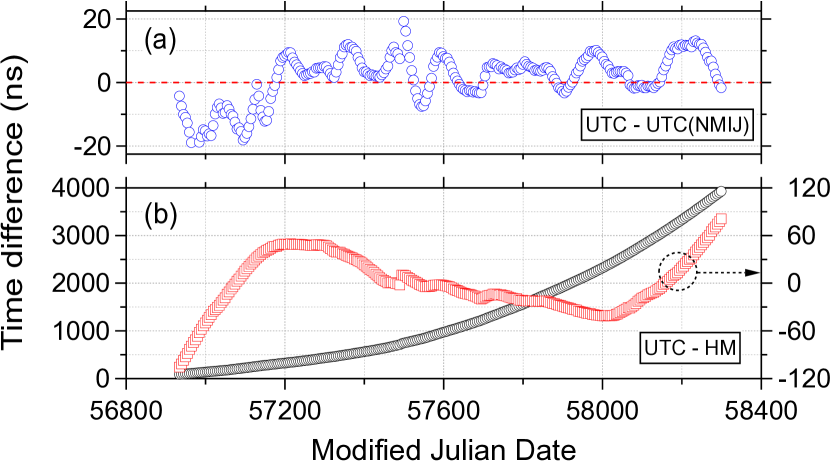
Figure 1: (a) Time difference between UTC and UTC(NMIJ) over about the last 3.5 years (the [UTC $-$ UTC(NMIJ)] values) reported in Circular-T. (b) Time difference between UTC and the master oscillator (hydrogen-maser) of UTC(NMIJ) (the [UTC $-$ HM] values, open circles, the left axis), and that after subtracting the quadratic component from the [UTC $-$ HM] values (open red squares, the right axis). In both figures, all vertical axes are in nanosecond units.

II Computational method

Let us explain the data treated in this study and clarify the question to be solved. We firstly obtained the time difference between UTC and HM (the [UTC $-$ HM] values) as shown in Fig. 1(b) (open circles, the left axis) with the same range as the [UTC $-$ UTC(NMIJ)] values as described above, by summing the [UTC(NMIJ) $-$ HM] values recorded in our group and the [UTC $-$ UTC(NMIJ)] values reported in Circular-T. As seen in Fig. 1(b), the [UTC $-$ HM] values appear to have a quadratic component as a function of MJD. Figure 1(b) also shows the residual component after subtracting the quadratic component from the [UTC $-$ HM] values (open red squares, the right axis). The residual component shown in Fig. 1(b) changes between about -100 ns and 80 ns, whereas UTC(NMIJ) is within 20 ns of UTC as shown in Fig. 1(a). This fact suggests that the residual component as shown in Fig. 1(b) is corrected by the frequency adjustment of the HM, and needs to be predicted precisely with a view to improving the synchronous accuracy of UTC(NMIJ) relative to UTC. We thus predicted the residual component with deep learning.

To this end, we employed a one-dimensional convolutional neural network (1D-CNN). CNNs are used not only for the various types of image processing Sze et al. (2017) but also for the analysis of the time series data as in this study Längkvist, Karlsson, and Loutfi (2014). Although several studies on the prediction of the time difference between UTC and time scales using neural networks have been reported Miczulski and Sobolewski (2017); Lei et al. (2017), the effectiveness of the CNNs have not been explored. Figure 2 shows the training flow of the 1D-CNN and the structure of that implemented in this study. The CNNs are essentially a stack of the convolutional layers, which are composed of plural neurons, and the part of neurons is coupled to the ones in another convolutional layer with certain weights. In the convolutional layers, the features of the data are recognized by using the filters. The prototype convolutional layers are linear systems, because their outputs constitute the multiplication and addition of the input data and the filters. To enhance the expressiveness of the CNNs the non-linear activation functions are introduced following the convolutional layers. The goal of deep learning is to generalize the ANNs, that is, to realize ANNs with good performance even for data it has never seen before. For this purpose, the loss values, i.e., the differences between the outputs of the ANN and their corresponding actual values, are calculated by using the loss function in the training process. The ANNs including CNNs are basically a composition of multiple functions with many weights. The optimizer updates the weights so as to minimize the loss values.

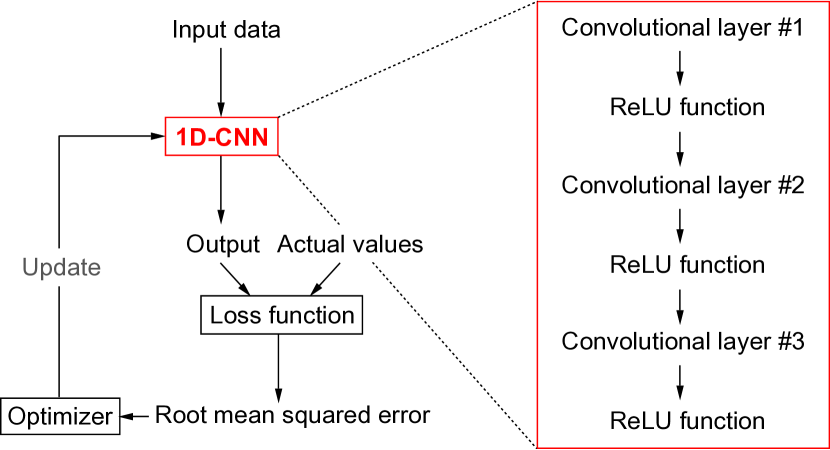
Figure 2: Training flow of the 1D-CNN and the structure of that implemented in this study. In the present training, the root mean squared error was calculated as the loss value and the Adaptive moment estimation (Adam) algorithm Goodfellow, Bengio, and Courville (2016); Le et al. (2011) was used as the optimizer. All convolutional layers were followed by the Rectified Linear Unit (ReLU) function as the non-linear function.

The total number of the discrete time difference data between UTC and HM shown in Fig. 1(b) was 274 and we denote this data as $d_{i}\ (i=1,2,...,274)$. We normalized the data by the maximum of the absolute value such that $x_{i}=d_{i}/|d_{\text{max}}|$. The initial 51% of the normalized data, noted by ${\bf x}^{\text{trn}}=[x_{1},\ x_{2},\ ...\ ,x_{141}]$, were fed into the 1D-CNN for the training. The features of the input data were recognized in the three convolutional layers by using three filters of which size were 1 $\times$ 4, 1 $\times$ 3 and 1 $\times$ 3. All convolutional layers were followed by the Rectified Linear Unit (ReLU) functions Goodfellow, Bengio, and Courville (2016), which returns zero if the input values are zero or less, but it returns that values for positive input values. The ReLU function induces non-linearity and sparsity for better training Glorot, Bordes, and Bengio (2011). The root mean squared error $E_{\text{RMS}}^{\text{trn}}$ was calculated as the loss value in the present training, which is defined as

$$E_{\text{RMS}}^{\text{trn}}=\sqrt{\frac{1}{n_{\text{trn}}}\ {\displaystyle\sum_{i=1}^{n_{\text{trn}}}\left(x_{i}^{\text{pred}}-x_{i}\right)^{2}}},\$$ (1)

where $n_{\text{trn}}$, $x_{i}^{\text{pred}}$ are the number of the training data, $i$-th prediction by the 1D-CNN in the training, such that $x_{i}^{\text{pred}}=f({\bf x}^{\text{trn}},{\bf W})$, and W is the weights of the 1D-CNN to be optimized in the training. From the comparison between some optimizers, the Adaptive moment estimation (Adam) algorithm Goodfellow, Bengio, and Courville (2016) was selected as the optimizer. The Adam algorithm is widely used in the CNNs due to its high-efficiency and low computational cost Le et al. (2011). The computer program was written with MATLAB programming language MAT .

III Results and discussions

III.1 Results of training

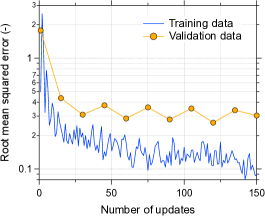
Figure 3: The results of the training, i.e., the root mean squared error of the training data and that of the validation data as a function of the number of weights updates with a logarithmic scale of the vertical axis.

Figure 3 shows the results of the training of the 1D-CNN, i.e., $E_{\text{RMS}}^{\text{trn}}$ of the training data and that of the validation data as a function of the number of weights updates with a logarithmic scale of the vertical axis. $E_{\text{RMS}}^{\text{trn}}$ of the training data gradually decreased and changed slightly after about the 50th update. This indicates that the weights of the 1D-CNN were optimized to the training data after about the 50th update. In the present study, the 12% of normalized data (33) were used as the validation data, that were not used in the training. The training of the 1D-CNN involves some parameters, e.g., the number of the convolutional layers and filters, the types of non-linear functions and optimizers. All of these parameters were determined so as to converge $E_{\text{RMS}}^{\text{trn}}$ of the validation data. As for $E_{\text{RMS}}^{\text{trn}}$ of the validation data shown in Fig. 3, similar behavior to that of the training data was observed after about the 25th update. One point to be noted as regards the training is the overfitting Goodfellow, Bengio, and Courville (2016), which happens when the ANNs are tuned only for the training data and do not generalize to unseen data. Once overfitting occurs, $E_{\text{RMS}}^{\text{trn}}$ of the validation data is expected to exhibit monotonically increasing trend starting from a certain update. Although there are some method to avoid the overfitting, we employed the L2 regularization and the early stopping method Goodfellow, Bengio, and Courville (2016). $E_{\text{RMS}}^{\text{trn}}$ of the validation data shown in Fig. 3 indicates that overfitting has not occurred in the present 1D-CNN. From the above, it is reasonable to consider that the training of the 1D-CNN had been conducted properly.

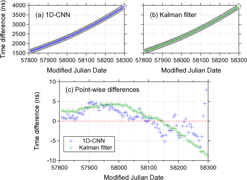
Figure 4: Typical prediction result obtained by the 1D-CNN (a) and the Kalman filter (b). In both Figs. (a) and (b), the test data are shown as the open circles. The point-wise differences between the test data and the prediction results obtained by two methods are shown in (c).

III.2 Prediction results and discussions

The typical prediction result obtained by the trained 1D-CNN is shown in Fig. 4(a) (blue crosses). In Fig. 4(a), the actual data (open circles), which were used as neither the training nor the validation data, are also shown and we hereinafter refer to this data as the test data. Figure 4(b) shows the prediction by the Kalman filter (green crosses) as mentioned later and Fig. 4(c) shows the point-wise differences between the test data and the predictions obtained by two methods. The predictions by the 1D-CNN and the Kalman filter were performed by repeating the short-term prediction over the whole data as follows; 5 points of test data (open red circles in Fig. 1(b)) were fed into the 1D-CNN and the Kalman filter and they predicted one point ahead. Both prediction results shown in Figs. 4(a) and (b) were eventually obtained by summing the predicted residual components and the subtracted quadratic component. The procedure for the prediction as described above means that the results of the previous predictions were not taken into account in each prediction cycle. In this sense, we have to admit that the performance of the present 1D-CNN as a predictor is at an early stage. As can be seen from Fig. 4(c), the point-wise differences between the test data and the predictions by two methods tended to increase in the latter half of the predictions. This may be related to the environmental variations of the room where the HM is located. In fact, the room temperature of the range from MJD 58200 to 58300 significantly fluctuated compared to the other range. This may resulted in the discrepancy between the test data and the prediction results. In other words, the prediction may be improved by considering the environmental variations of the room where the HM is located.

As described above, we also performed the prediction by using the Kalman filter on the same training and test data. The Kalman filter is a linear iterative method for modeling the continuous observables affected by the random noise Harvey (1990). There exist some studies on the prediction of the time difference between UTC and the atomic clocks with the Kalman filter Davis, Shemar, and Whibberley (2011). Let us calculate the root mean squared error of the results of the predictions $E_{\text{RMS}}^{\text{pred}}$. $E_{\text{RMS}}^{\text{pred}}$ is defined as

$$E_{\text{RMS}}^{\text{pred}}=\sqrt{\frac{1}{n_{\text{pred}}}\ {\displaystyle\sum_{j=1}^{n_{\text{pred}}}\left(x_{j}^{\text{pred}}-x_{j}^{\text{test}}\right)^{2}}},\$$ (2)

where $n_{\text{pred}}$, $x_{j}^{\text{pred}}$ and $x_{j}^{\text{test}}$ are the number of the predicted data, the results of predictions and the test data, respectively. $E_{\text{RMS}}^{\text{pred}}$ of the predictions obtained by two methods shown in Figs. 4 were calculated to be,

$$\text{1D-CNN : }\approx 3.0\ \text{ns},\ \text{Kalman filter : }\approx 3.8\ \text{ns}.$$

In the results of repeating the predictions, we observed improvement in $E_{\text{RMS}}^{\text{pred}}$ of the prediction obtained by the 1D-CNN compared with that obtained by the Kalman filter. The 1D-CNN has been designated to exploit complex dependencies among input variables via many layers of non-linear operators for the prediction. On the other hand, the Kalman filter recursively performs a conditional probability estimation, and this method is commonly anticipated to be optimal under the Gaussian model assumption. In other words, the 1D-CNN exploited larger hypothesis space than that of the Kalman filter for the prediction. The improvement in $E_{\text{RMS}}^{\text{pred}}$ of the prediction by the 1D-CNN as shown above can be attributed to the higher expressiveness of the 1D-CNN than that of the Kalman filter, i.e., high non-linearity and superior ability to exploit complex relationships between input variables. Furthermore, the difference in the mathematical assumptions between two methods as described above also reflected in the error trend in Fig. 4(c); while the prediction result obtained by the 1D-CNN (blue crosses in Fig. 4(c)) was more wiggling than that obtained by the Kalman filter, the prediction result obtained by the Kalman filter (green crosses in Fig. 4(c)) exhibits a mostly continuous and monotonic curve, which is consistent with recursive model updating algorithm of the Kalman filter. Although more investigations are required to conclude that the 1D-CNN can work as a good predictor, the present results suggest that our new computational approach may accordingly provide a useful method for improving the synchronous accuracy of UTC(NMIJ) relative to UTC. We are now working on the detail investigations towards establishing the reliable method for predicting the [UTC $-$ HM] values and the results will be comprehensively discussed in our forthcoming paper including the prediction by the Kalman filter.

IV Conclusion

We have predicted the time difference between UTC and HM, which is used as a master oscillator for UTC(NMIJ) by using a 1D-CNN, and observed the improvement in the accuracy of prediction compared with that obtained by the Kalman filter. The prediction may be improved by considering the environmental variations of the room where the HM is located. In addition, the present study focused on not the efficiency of the prediction but the accuracy of the prediction, therefore the present 1D-CNN has not been optimized regarding the speed of the computation. We will address the points as above in the near future towards establishing the deep learning based method for improving the synchronous accuracy of UTC(NMIJ) relative to UTC. It should be emphasized that the method discussed in this paper will also be available not only for improving the synchronous accuracy of UTC(NMIJ) relative to UTC but also for other UTC($k$) time scales. Such versatility and application potential attract much interests.

References

- Arias, Panfilo, and Petit (2011) E. F. Arias, G. Panfilo, and G. Petit, Metrologia 48, S145 (2011).
- Audoin and Guinot (2001) C. Audoin and B. Guinot, The Measurement of Time: Time, Frequency and the Atomic Clock (Cambridge University Press, Cambridge, 2001).
- (3) BIPM Time Department, “BIPM Annual Report on Time Activities (2017),” (URL: http://www.bipm.org/en/bipm/tai/annual-report.html).
- Sze et al. (2017) V. Sze, Y. Chen, T. Yang, and J. S. Emer, Proceedings of the IEEE 105, 2295 (2017).
- Längkvist, Karlsson, and Loutfi (2014) M. Längkvist, L. Karlsson, and A. Loutfi, Pattern Recognition Letters 42, 11 (2014).
- Miczulski and Sobolewski (2017) W. Miczulski and Ł. Sobolewski, IEEE Transactions on Instrumentation and Measurement 66, 2136 (2017).
- Lei et al. (2017) Y. Lei, M. Guo, Dan-dan Hu, Hong-bing Cai, Dan-ning Zhao, Zhao-peng Hu, and Yu-ping Gao, Advances in Space Research 59, 524 (2017).
- Goodfellow, Bengio, and Courville (2016) I. Goodfellow, Y. Bengio, and A. Courville, Deep Learning (MIT Press, Cambridge, MA, 2016).
- Le et al. (2011) Q. V. Le, J. Ngiam, A. Coates, A. Lahiri, B. Prochnow, and A. Y. Ng, in Proceedings of the 28th International Conference on International Conference on Machine Learning, ICML’11 (Omnipress, USA, 2011) pp. 265–272.
- Glorot, Bordes, and Bengio (2011) X. Glorot, A. Bordes, and Y. Bengio, in Proceedings of the Fourteenth International Conference on Artificial Intelligence and Statistics, Proceedings of Machine Learning Research, Vol. 15, edited by G. Gordon, D. Dunson, and M. Dudík (PMLR, Fort Lauderdale, FL, USA, 2011) pp. 315–323.
- (11) MATLAB version R2019a, The MathWorks Inc., Natick, Massachusetts, 2019.
- Harvey (1990) A. C. Harvey, Forecasting, Structural Time Series Models and the Kalman Filter (Cambridge University Press, Cambridge, 1990).
- Davis, Shemar, and Whibberley (2011) J. A. Davis, S. L. Shemar, and P. B. Whibberley, in 2011 Joint Conference of the IEEE International Frequency Control and the European Frequency and Time Forum (FCS) Proceedings (2011) pp. 1–6, and references therein.