Analysing the Main Belt asteroid distributions by wavelets

Abstract

We perform statistical wavelet analysis of the Main Belt asteroids, seeking statistically significant asteroid families. The goal is to test the new wavelet analysis algorithm and to compare its results with more traditional methods like the hierarchic clustering. We first consider several 1D distributions for various physical and orbital parameters of asteroids. Then we consider three bivariate distributions for the three orbital parameters $(a,e,i)$ taken pairwisely. The full 3D analysis of this space is not available here, but based on the 2D results we perform a disentangling of overlapped 2D families and derive total of $44$ 3D families with confirmed statistical significance.

1 Introduction

First attempts to find asteroid families date back to XIX century, although the discovery of new asteroids was rather slow that time, compared to the contemporary rate. In 1876, based on just about 150 asteroids, D. Kirkwood noticed about 10 asteroid groups, each containing just 2-3 members moving along similar orbits. It was suggested that asteroids in such groups may have a common origin, e.g. are fragments of larger disrupted bodies. F. Tisserand continued Kirkwood attempts, composing a list of 417 asteroids (1891), and also introducing a formal orbital classification characteristic now well-known as the Tisserand invariant $T_{J}$ (see Hirayama, 1922). The number of asteroid families grew as new asteroids were discovered. However, no other factors supported the common origin within a family, except for orbit closeness. Therefore, the physical relationship of such asteroids often remained too disputable.

Later on, Hirayama (1918) noticed that it might be not reasonable to compare contemporary orbits of asteroids for that goal. On a long time scale, planetary perturbations may change orbits a lot, even if asteroids indeed were fragments of the same body in some past and had close orbits initially. This motivation leaded K. Hirayama to the idea of invariant orbital elements that would remain (nearly) constant regardless of the planetary perturbations. Hirayama constructed such invariant elements based on the Lagrange perturbation theory and introduced them as ‘proper elements’, assuming that asteroids from the same family inherited them from their progenitors, should the latter existed in some past. The proper elements remain very useful to identify the asteroid families.

Of course, the fragments may attain some minor additional velocities after a disruption of a larger body, still resulting in some minor spread even in terms of the proper elements. Moreover, the boundaries of such families are typically rather vague, merging with the background distribution. Because of this, the population even within well-known asteroid families is difficult to determine strictly, and it is often uncertain whether an asteroid belongs to a particular family or not.

Although Hirayama introduced the notion of ‘asteroid family’ in the sense of an asteroid group probably sharing common origin, nowadays this term is relatively ambiguous. Even the closeness of proper elements of some asteroids does not guarantee their common origin. Other explanations are also possible, for example the mean-motion resonance (MMR). In this case an MMR may serve as an orbital ‘trap’ capturing objects that would not otherwise have any common history. Possible example might be e.g. the Hilda family (Brož and Vokrouhlický, 2008), though presently it is deemed to be a widely eroded superfamily of common origin (Milani et al, 2017). In some part, the question of common origin of asteroids may be resolved using their spectral classification, but given the current high discovery rate it is not feasible to perform an accurate taxonomic analysis of all asteroids (Masiero et al, 2015). Also, the disrupted progenitor body could be so large that its fragments would appear chemically different.

Therefore, in this work under a ‘family of asteroids’ we understand a group of objects simply having close orbital or physical parameters. Such a property may suggest a hint that these asteroids could have common evolutionary origin, but does not guarantee that.

Presently, the most popular method of asteroid family identification is the hierarchic clustering method (HCM hereafter), which looks for objects with a small distance between each other or from a main asteroid (Zappalà et al, 1990). The advantage of this method is that it does not explicitly specifies any assumptions about the shape of the asteroid family in the space of orbital parameters. Also, it can be relatively easily extended to higher dimensions (larger number of the parameters involved). Its main disadvantage, which becomes increasingly important when more and more small asteroids are discovered, is the effect of ‘chaining’. In case of a collision, small fragments are thrown away with larger velocities, and also they are subject to a stronger Yarkovsky effect. Therefore, they spread further in the parametric space, revealing a tendency to distribute more uniformly and create ‘bridges’ between different families. This issue is currently solved using rather artificial methods, e.g. by cutting the parametric space into distinct domains. Finally, the results may differ depending on the orbital distance metric (Nesvorný et al, 2015).

Yet another method of asteroid family identification is wavelet analysis, which was used previously but did not attain the same popularity so far. Based on a sample of $\sim 12000$ asteroids, Zappalà et al (1995) concluded that HCM and wavelet analysis methods yield similar results. Both methods detected the same families, though the number of asteroids in a family was different. We believe that the wavelet analysis was abandoned after that because, firstly, it was a pretty young technique at that time (especially in what concerns statistical tasks), and secondly, because it is more computationally demanding.

But now the wavelet analysis gained a considerably wider attention, whereas the computing hardware progressed greatly. Also, the mathematical theory of the statistical flavours of the wavelet analysis was significantly improved, compared to 1990s. For example, in (Baluev, 2018) a new algorithm was presented, targeting the analysis of 1D statistical distributions. It is not a cluster detection algorithm in the common sense, because it has a more wide range of applications than just clusters identification. In particular, it allows to detect distribution gaps as well as clusters, and also to investigate the finely-resolved distribution shape inside the cluster (or gap). Contrary to methods from (Zappalà et al, 1995), the primary attention is paid to the optimised statistical sensitivity to allow a detection of patterns with smaller S/N ratio. Moreover, the significance of the detected patterns is expressed in the traditional and intuitive ‘p-value’ or ‘n-sigma’ notation. In fact, the algorithm from (Baluev, 2018) represents a tool to clean the shot noise (or finite sample noise) from an estimated density function, based on certain predefined statistical tolerance, and aiming to detect patterns of certain shape determined by the selected wavelet.

This technique is under a continuous development, for example the 2D analysis tool was constructed recently (Baluev et al, 2020a), and further generalisations are also possible. In this work, we aim to further develop this wavelet analysis method and the associated software, presenting our analysis results regarding the numerous sample of the Main Belt asteroids.

Notice that we do not advocate that wavelet analysis may (or is expected to) supersede the HCM in some concern. Rather, they represent two qualitatively different methods of the analysis. Their detailed comparison in terms of reliability and efficiency is definitely interesting, but this is too big task for this paper. Instead, we only plan to provide some field testing of our wavelet algorithm in the asteroid analysis task.

Very recently, machine learning was also introduced for asteroid family detection (Carruba et al, 2019), though in this work we omit detailed discussion of methods of this type.

In Sect. 2 we discuss some details about proper elements and the asteroid families. In Sect. 3 our asteroid samples are discussed. In Sect. 4 we give several basic details about our wavelet analysis algorithm. In Sect. 5 we analyse 1D distributions of various asteroid parameters. In Sect. 6 we present results of the 2D analysis and a list of detected asteroid families in the 3D space of semimajor axis, eccentricity, and inclination.

2 Scientific context regarding the proper elements

The classic definition says that proper orbital elements are quasi-integrals of the motion equations, so they remain almost constant in time (Knežević et al, 2002). Proper elements can be obtained after removal of short- and long-period perturbations from their osculating counterparts and hence represent some “mean” motion characteristics. (Hirayama, 1918), who introduced the concept of proper elements, also showed that some asteroids tend to accumulate into groups in the plains $(a,e_{p})$ and $(a,i_{p})$, where $e_{p}$ and $i_{p}$ are proper eccentricity and proper inclination. He supposed that such groups, or families, formed as a result of disintegration of a large parent body. Each family was named based on its largest member object.

Hirayama introduced in his works the notions of a proper eccentricity and proper inclination, but not of the proper semimajor axis, because the latter one has no secular perturbations (Murray and Dermott, 1999). Nevertheless, the contemporary notion of proper semimajor axis includes averaging with respect to short-period perturbations (Knežević et al, 2002).

In the classic theory of perturbations, the eccentric variables $h=e\sin{\varpi}$ and $k=e\cos{\varpi}$ vary along a nearly-circular curve in the 2D plane, with a constant angular velocity. Then, the proper eccentricity has an easy interpretation. The center of the circle (the so-called forced eccentricity) would move along a complicated trajectory defined by secular perturbations (and depending on semimajor axes), while the radius of the circle is equal to the proper eccentricity, which is defined by initial conditions and thus represents a fundamental orbital parameter. An analogous interpretation can be used for the inclinational parameters $\sin i$ and $\Omega$ (Murray and Dermott, 1999, chap. 7).

Two methods are currently used to determine the proper elements: the analytic and so-called synthetic ones (Knežević et al, 2002). The first method is based on the perturbation theory and involves the computation of averaged elements using canonical transform to remove short- and long-periodic terms. Synthetic theory involves the integration of asteroid and planetary motion and filtering of periodic perturbations. After that the primary harmonics are determined by means of the Fourier analysis. These primary harmonics are the proper elements.

The synthetic method is now more suitable thanks to its better accuracy (Knežević et al, 2002). Additionally, the analytic removal of short- and long-period term becomes difficult near the resonances, so the synthetic method performs better in such conditions. The resonant proper elements may be obtained by means of resonance averaging.

Figure 1: Diagram for semimajor axis – eccentricity (osculating) for the Main Belt. We can see vertical bands marking the mean-motion resonances.

In Fig. 2 that shows a 2D distribution of asteroids in the $a$–$e$ plane, we can see multiple vertical bands, which mark various mean-motion resonances that dominate in the dynamical regime of the relevant asteroids. We notice that our 1D wavelet analysis algorithm (Baluev, 2018) suits quite well to locate such 1D bands.

Unfortunately, neither analytic nor synthetic method can process the secular resonances well, e.g. the cases when two orbits have synchronized precession rates (for their perihelia, or ascending nodes, or both). Such asteroids have less accurate estimations of proper elements (especially proper eccentricity). In this work we removed from our analysis the asteroids in the secular resonance $g+g_{5}-2g_{6}$, which are explicitly identified in AstDys.

Figure 2: Diagram for proper semimajor axis – proper eccentricity for the Main Belt. Contrary to Fig. 1, we can clearly see compact spots additionally to vertical bands.

As we can see from Fig. 2, the proper elements allow to identify many asteroid families even by a plain look. However, some more subtle families may be more hard to reveal in the background distribution, emphasizing the value of a sophisticated statistical analysis in this task.

3 Asteroid samples

Though there were attempts to reveal families among the trans-Neptune objects (Snodgrass et al, 2012), such objects are relatively few, and their orbital elements are less accurate, so in this work we limited ourselves mostly to the Main Belt.

The osculating orbital elements and physical parameters were taken from the Lowell observatory catalog astorb.dat as of February 2019 . For our analysis we used only numbered asteroids in the range from $0.7$ AU to $7$ AU in semimajor axis. In these limits we had $523175$ objects with known eccentricity, inclination, and absolute magnitude. Unfortunately, the color index B-V was known only for $941$ asteroids, while the diameter was known for $2139$ ones. Nonetheless, we tried to analyse the distributions for all these physical parameters too, since based on the previous experience (Baluev and Shaidulin, 2018), samples containing 1-2 thousand of objects still may reveal statistical clusters.

The proper elements are available in the AstDys database . AstDyS is currently managed by the following consortium: Department of Mathematics, University of Pisa, Italy; IASF-INAF Rome, Italy; SpaceDyS srl, Cascina, Italy, and others. It supplies information about numbered asteroids, with a detailed description provided by Knežević and Milani (2003). The proper orbital elements are determined in the semimajor axis range from $1.7$ AU to $4.0$ AU, with $464746$ asteroids in total (after removal of objects in secular resonances). For our analysis we used proper elements derived by the synthetic method.

In Table LABEL:AstDysFamilies we give the asteroid families detected so far in AstDys, including the primary object, number of asteroids, and proper element ranges. See also Milani et al (2014, 2017). Below we use this list as a reference for comparison with our results. The star following the family name indicates that this family was confirmed by our wavelet analysis (see Table LABEL:residual below). If there are multiple stars following the same name this means that we detected several subfamilies by wavelets.

Table 1: Currently known AstDys asteroid families.

Core object	$N$	$a_{\min}$	$a_{\max}$	$e_{\min}$	$e_{\max}$	$\sin i_{\min}$	$\sin i_{\max}$
434 Hungaria *	1879	1.883	1.988	0.05	0.097	0.343	0.378
883 Matterania	169	2.213	2.259	0.14	0.152	0.092	0.102
2076 Levin *	1534	2.251	2.325	0.129	0.153	0.088	0.106
4 Vesta *	10612	2.256	2.482	0.08	0.127	0.1	0.133
1338 Duponta	133	2.259	2.302	0.119	0.13	0.075	0.091
298 Baptistina	176	2.26	2.288	0.146	0.161	0.1	0.114
25 Phocaea	1248	2.26	2.417	0.159	0.265	0.366	0.425
135 Hertha	15983	2.288	2.479	0.134	0.215	0.026	0.059
163 Erigone *	542	2.331	2.374	0.2	0.219	0.08	0.098
20 Massalia *	7820	2.334	2.474	0.145	0.175	0.019	0.034
5026 Martes *	481	2.368	2.415	0.2	0.217	0.082	0.096
302 Clarissa *	236	2.385	2.421	0.104	0.111	0.056	0.06
6769 Brokoff	58	2.398	2.431	0.148	0.155	0.051	0.056
752 Sulamitis	193	2.42	2.484	0.084	0.095	0.085	0.092
15 Eunomia	9856	2.521	2.77	0.117	0.181	0.203	0.256
194 Prokne	379	2.522	2.691	0.154	0.196	0.292	0.315
170 Maria	2958	2.523	2.673	0.067	0.128	0.231	0.269
480 Hansa	1162	2.538	2.731	0.001	0.102	0.364	0.385
1658 Innes *	775	2.544	2.627	0.164	0.185	0.121	0.142
3811 Karma	59	2.547	2.579	0.101	0.11	0.185	0.19
10369 Sinden	24	2.551	2.609	0.104	0.118	0.469	0.482
3815 König *	578	2.563	2.584	0.138	0.143	0.144	0.164
606 Brangäne *	325	2.571	2.597	0.178	0.183	0.165	0.168
145 Adeona *	2070	2.573	2.714	0.153	0.181	0.193	0.213
4203 Brucato	41	2.586	2.69	0.119	0.138	0.47	0.489
945 Barcelona	346	2.591	2.668	0.189	0.289	0.506	0.521
116763	24	2.612	2.652	0.236	0.246	0.463	0.468
3 Juno *	1693	2.622	2.7	0.227	0.245	0.225	0.239
569 Misa	647	2.623	2.694	0.169	0.184	0.034	0.045
7744	98	2.633	2.67	0.069	0.075	0.041	0.049
1547 Nele *	344	2.638	2.65	0.266	0.27	0.21	0.213
29841	65	2.639	2.668	0.052	0.059	0.033	0.04
17392	96	2.645	2.681	0.059	0.07	0.036	0.042
23255	12	2.655	2.7	0.095	0.113	0.46	0.469
2782 Leonidas	111	2.657	2.701	0.185	0.197	0.06	0.072
10955 Harig	918	2.671	2.762	0.005	0.026	0.1	0.113
12739	298	2.682	2.746	0.047	0.06	0.031	0.041
11882	87	2.683	2.711	0.059	0.066	0.031	0.04
110 Lydia	898	2.696	2.779	0.026	0.061	0.083	0.106
808 Merxia **	1263	2.705	2.81	0.125	0.143	0.08	0.093
410 Chloris	120	2.705	2.761	0.238	0.266	0.146	0.16
3827 Zdeněkhorský *	1050	2.705	2.768	0.082	0.096	0.08	0.094
21344	75	2.708	2.741	0.15	0.16	0.046	0.05
53546	81	2.709	2.735	0.169	0.174	0.247	0.251
14916	17	2.71	2.761	0.27	0.282	0.537	0.542
148 Gallia	137	2.71	2.812	0.114	0.15	0.42	0.43
847 Agnia **	3336	2.713	2.819	0.063	0.083	0.055	0.076
40134	16	2.715	2.744	0.223	0.235	0.429	0.44
93 Minerva *	2428	2.718	2.816	0.115	0.155	0.146	0.169
729 Watsonia	83	2.72	2.816	0.11	0.144	0.294	0.305
396 Aeolia *	529	2.728	2.752	0.163	0.171	0.057	0.062
668 Dora *	1742	2.744	2.812	0.188	0.204	0.128	0.143
2 Pallas	45	2.752	2.791	0.254	0.283	0.531	0.55
1128 Astrid *	548	2.754	2.817	0.045	0.053	0.008	0.019
1726 Hoffmeister *	2095	2.754	2.82	0.041	0.053	0.066	0.088
13314	241	2.756	2.804	0.17	0.183	0.069	0.079
18466 *	257	2.763	2.804	0.171	0.182	0.229	0.236
32418	81	2.763	2.795	0.255	0.261	0.152	0.156
1222 Tina	107	2.764	2.811	0.065	0.113	0.349	0.36
158 Koronis ****	7390	2.816	2.985	0.016	0.101	0.029	0.047
293 Brasilia *	845	2.832	2.874	0.118	0.133	0.256	0.264
18405	159	2.832	2.859	0.103	0.11	0.158	0.162
16286 *	94	2.846	2.879	0.038	0.047	0.101	0.111
1189 Terentia	80	2.904	2.936	0.07	0.075	0.192	0.194
845 Naëma *	375	2.914	2.962	0.029	0.041	0.205	0.209
179 Klytaemnestra *	513	2.946	3.015	0.051	0.081	0.147	0.16
221 Eos *	16038	2.948	3.211	0.022	0.133	0.148	0.212
283 Emma *	577	3.028	3.086	0.107	0.124	0.154	0.166
7468 Anfimov	49	3.031	3.075	0.087	0.091	0.059	0.061
3438 Inarradas	43	3.036	3.076	0.174	0.186	0.249	0.255
96 Aegle *	120	3.036	3.083	0.176	0.189	0.279	0.289
24 Themis **	5612	3.062	3.24	0.114	0.192	0.009	0.049
10 Hygiea	3145	3.067	3.242	0.1	0.166	0.073	0.106
21885	61	3.079	3.112	0.025	0.035	0.184	0.189
31 Euphrosyne	1385	3.082	3.225	0.149	0.231	0.431	0.459
1040 Klumpkea *	1815	3.083	3.175	0.176	0.217	0.279	0.304
780 Armenia	67	3.085	3.133	0.06	0.075	0.31	0.314
1298 Nocturna	186	3.088	3.22	0.105	0.124	0.103	0.125
159 Aemilia	62	3.091	3.131	0.111	0.117	0.084	0.09
31811	144	3.095	3.14	0.059	0.075	0.178	0.188
375 Ursula	731	3.095	3.241	0.057	0.13	0.264	0.303
5651 Traversa	56	3.097	3.166	0.111	0.129	0.231	0.241
43176	75	3.107	3.156	0.065	0.075	0.174	0.184
58892	20	3.113	3.154	0.152	0.163	0.3	0.308
8737 Takehiro	57	3.116	3.143	0.112	0.121	0.207	0.211
3330 Gantrisch *	1241	3.118	3.178	0.184	0.213	0.171	0.184
1118 Hanskya	116	3.133	3.249	0.034	0.059	0.252	0.267
22805	20	3.135	3.167	0.165	0.175	0.301	0.308
490 Veritas *	2139	3.143	3.197	0.048	0.08	0.151	0.173
7605	19	3.143	3.154	0.063	0.075	0.447	0.453
778 Theobalda *	574	3.155	3.199	0.239	0.261	0.243	0.253
3460 Ashkova	59	3.159	3.219	0.186	0.211	0.016	0.028
5931 Zhvanetskij	23	3.174	3.215	0.16	0.172	0.302	0.313
618 Elfriede	97	3.177	3.2	0.056	0.059	0.27	0.278
6355 Univermoscow	13	3.188	3.217	0.088	0.097	0.374	0.378
3025 Higson	17	3.188	3.221	0.059	0.066	0.366	0.378
1303 Luthera	232	3.192	3.237	0.106	0.144	0.31	0.337
895 Helio	50	3.194	3.225	0.168	0.183	0.437	0.446
69559	17	3.201	3.219	0.196	0.201	0.299	0.305
10654 Bontekoe	13	3.207	3.244	0.051	0.056	0.368	0.374
1101 Clematis	17	3.229	3.251	0.03	0.037	0.363	0.375
11097	33	3.274	3.275	0.23	0.28	0.014	0.038
45637	20	3.341	3.369	0.103	0.123	0.142	0.151
260 Huberta	26	3.41	3.464	0.079	0.089	0.099	0.108
87 Sylvia	191	3.458	3.567	0.046	0.074	0.162	0.179
909 Ulla	37	3.524	3.568	0.043	0.058	0.306	0.309
3561 Devine	19	3.962	3.962	0.127	0.133	0.149	0.156
1911 Schubart	531	3.964	3.967	0.158	0.224	0.039	0.056
153 Hilda	18	3.965	3.966	0.171	0.181	0.152	0.156
6124 Mecklenburg	78	3.966	3.967	0.186	0.212	0.146	0.159

4 Statistical wavelet analysis

We emphasize that in this work the notion “asteroid family” is understood in the statistical sense, that is as a group of objects that are statistically unlikely to originate from the randomness of the asteroid sample (from its shot noise). Therefore, such a group should be generated by some physical mechanism, but this does not necessarily suggests that these objects have common origin.

A self-consistent method perform wavelet analysis was presented in (Baluev, 2018). That first release handled several theoretic issues that had not a good solution before, and also involved wavelets of optimized shape, but that analysis tool targeted only 1D distributions. However, the first test application of this initial 1D method to exoplanetary population revealed several rather interesting results (Baluev and Shaidulin, 2018). In particular, hints of a previously unknown subtle family of giant exoplanets was detected, possibly related to the iceline accumulation effect in a protoplanetary disk. Finally, a 2D generalization of this algorithm was presented in (Baluev et al, 2020a). This analysis is based on isotropic radially symmetric wavelets, so it requires that two input parameters in the 2D sample are at least physically and numerically comparable (like e.g. two coordinates in the Euclidean space).

When processing exoplanetary samples that contained $\sim 10^{3}$ objects at most, it was not possible to derive entirely reliable and convincing results. For example, the formal significance of the exoplanetary family mentioned above was in the range $2-3$ sigma, i.e. its interpretation is still probabilistic. However, the Main Belt asteroids form a much larger sample containing between $10^{5}$ and $10^{6}$ objects. This should allow much more statistically reliable conclusions and more convincing detections.

For the full mathematical details of the wavelet analysis algorithm the reader is referred to (Baluev, 2018) and (Baluev et al, 2020a). Here we omit these details, only giving a few general ideas of the method.

First of all, the continuous wavelet transform (or CWT) is defined as

$$Y(s,b)=\int\limits_{\mathbb{R}^{n}}f(x)\psi\left(\frac{x-b}{s}\right)\,dx.$$ (1)

This assumes a general $n$-dimensional task, where $n=1$ or $n=2$ refers to the dimension of $x$ and of the shift parameter $b$. The scale parameter $s$ is always scalar here. The wavelet $\psi$ is assumed radially-symmetric for $n=2$, so it is actually a function of the length of its vector argument. Notice that the scale parameter is usually denoted as $a$, but we changed it to $s$ in order to avoid mixing it with the semimajor axis below.

The CWT can be inverted using the following general inversion formula:

$$f(x)=\frac{1}{C_{\psi\gamma}}\int\limits_{0}^{\infty}\frac{ds}{s^{2n+1}}\int\limits_{\mathbb{R}^{n}}Y(s,b)\gamma\left(\frac{x-b}{s}\right)\,db,$$ (2)

where $\gamma$ is a largerly arbitrary inversion kernel. Although the most popular version of (2) involves $\gamma=\psi$, it is possible to consider other $\gamma$ as well, resulting in certain useful specific properties of the inversion formula. The constant $C_{\psi\gamma}$ in (2) depends solely on the choice of $\psi$ and $\gamma$.

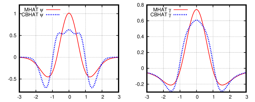
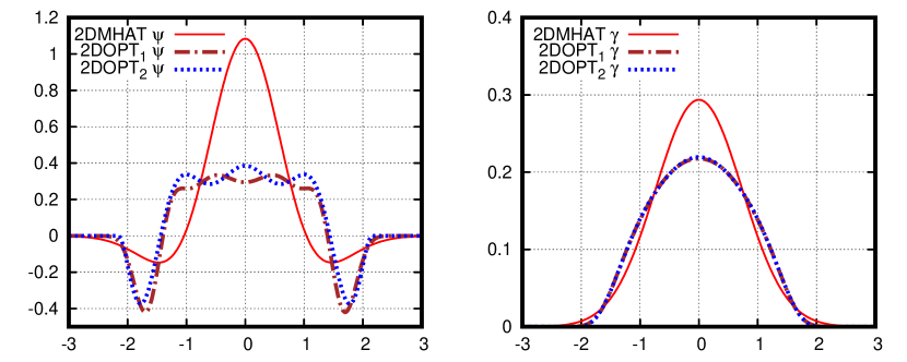
Figure 3: The optimized wavelet function $\psi$ for the CBHAT and 2DOPT wavelets and their optimal reconstruction kernels $\gamma$, compared to the classic 1D and 2D MHAT wavelets with their optimal $\gamma$.

We shape of the wavelet function $\psi$ is rather arbitrary and largerly depends on the goals of the analysis. In our work we will use optimized wavelets that allow to simultaneously minimize the noise level and improve the noise gaussianity. Such 1D and 2D wavelets, named as CBHAT (‘cowboy hat’) and 2DOPT, were derived in (Baluev, 2018; Baluev et al, 2020a), and are plotted in Fig. 3. Notice that they are different from the famous classic MHAT wavelet that does not suit in our task because it generates bad noise properties. Notice that we have two very close versions of 2DOPT, among which we select 2DOPT₂ (and thus omit this index hereafter). All these wavelets are such that $Y(s,b)$ represents a smoothed second derivative or a smoothed Laplacian of $f(x)$, with smoothing scale controlled by $s$. In Fig. 3 we also plot optimized inversion kernels $\gamma$ that allow to minimize the noise in the reconstructed $f(x)$.

We aim to apply the CWT to the 1D or 2D probability density function p.d.f. $f(x)$. However, this function is not observed directly, so the formulae (1) and (2) cannot be used at this stage. What we have in practice in place of $f(x)$ is the sample $\{x_{i}\}_{i=1}^{N}$, and hence we may only construct a statistical estimate for the CWT:

$$\tilde{Y}(s,b)=\frac{1}{N}\sum_{i=1}^{N}\psi\left(\frac{x_{i}-b}{s}\right).$$ (3)

Notice that the CWT itself, as defined in (1), is a mathematical expectation of $y=\psi[(x-b)/s]$, where $s$ and $b$ are parameters, so in (3) involves plainly corresponding sample mean of the same $y$. We therefore refer to (3) as to sample wavelet transform (SWT).

This is the point where the noise appears. The SWT is a noisy quantity since it is defined on the basis of a finite sample. It is easy to define the sample variance $\tilde{D}$ in the way similar to (3). Finally, we can construct the normalized test statistic

$$z(s,b)=\frac{\tilde{Y}(s,b)-Y(s,b)}{\sqrt{\tilde{D}(s,b)}},$$ (4)

which has asymptotically (for large $N$) the standard Gaussian distribution (mean zero, variance unit). Notice that we can substitute here any comparison model $Y_{0}$ in place of $Y$. Basically, our formal goal is to test whether some null hypothesis $Y=Y_{0}$ is statistically consistent or not.

The test statistic $z(s,b)$ is the central testing quantity that allows to derive whether the wavelet coefficient (the value of $\tilde{Y}$) is statistically sound at the given $(s,b)$. The typical noise would imply $z$ of the order of unit, while a large $z$ indicates a statistically significant inconsistency between the adopted comparison model $Y_{0}$ and the actual sample distribution. The Gaussian asymptotic distribution of $z$ can be used to construct a formal statistical test.

However, the reader is cautioned that it is inadequate to apply such approach literally if multiple $(s,b)$ points are tested (which is typically the case). We usually investigate a wide domain $\mathcal{D}$ in the $(s,b)$-plane, so the actual compound test basically involves multiple elementary tests per independent $z$-values. In such a case it is mandatory to apply some statistical correction for multiple testing. We put a special emphasis on this issue because it was often ignored so far in many other works, thus resulting in a drastically increased level of false positives among the detected wavelet coefficients.

In our framework, the multiple testing issue can be handled neatly if we consider the extreme value statistic instead of the single-value ones. Namely, what we test in actuality is the maximum deviation

$$z_{\max}=\max_{(s,b)\in\mathcal{D}}|z(s,b)|$$ (5)

instead of the particular $z(s,b)$ values. The distribution function of $z_{\max}$ is non-Gaussian, but it can be characterized analytically as an extreme value distribution of a Gaussian random field $z(s,b)$. This work was done in (Baluev, 2018; Baluev and Shaidulin, 2018), resulting in the following tail approximation

$$\mathrm{FAP}(\zeta)\equiv\Pr\{z_{\max}>\zeta\}\lesssim 2W_{00}\zeta^{n}e^{-\frac{\zeta^{2}}{2}}.$$ (6)

This formula connects the false alarm probability (FAP) with the maximum observed $z$-level. If the resulting $\mathrm{FAP}(z_{\max})$, computed for the actually observed $z_{\max}$, is smaller than a conventional threshold level (say, $1$ per cent or any) then the deviation is treated significant and the comparison model $Y_{0}$ disagrees with the sample. The coefficient $W_{00}$ depends on the wavelet $\psi$ and on the domain $\mathcal{D}$, and it can be computed numerically together with the SWT. Importantly, formula (6) has the shape of an approximate upper bound, so its possible inaccuracies should not lead to understated $\mathrm{FAP}$ (overstated significance). If the right hand side of (6) is below some $\mathrm{FAP}_{\rm thr}$ than the actual $\mathrm{FAP}$ is also below than this threshold.

Concerning the domain $\mathcal{D}$, it can be chosen rather arbitrary. In fact, it accumulates our prior assumptions, where we expect to find a signfificant wavelet coefficient, and where not. However, this domain cannot be arbitrarily large. In any case, it should be restricted to the domain where $z(s,b)$ is satisfactorily Gaussian, because it was our substantial assumption used to compute the FAP approximation (6). We typically expand $\mathcal{D}$ to this widest range, while the normality is verified using certain formalized criterion (Baluev, 2018; Baluev et al, 2020a).

Our statistical test based on (6) only allows to decide whether some given comparison model $f_{0}/Y_{0}$ agrees with the sample or not. However, this might appear not enough for our goals, because we would also like to learn, how the p.d.f. $f(x)$ should look to satisfy this restriction. In other word, we should construct some most economic p.d.f. model not violating the significance test. This is achieved through an iterative scheme with a single iteration layed out below:

$$f_{n}(x)\stackrel{{\scriptstyle\rm{CWT}}}{{\longmapsto}}Y_{n}(s,b)\stackrel{{\scriptstyle\rm{noise\ thresholding}}}{{\longmapsto}}Y_{n,\rm thr}(s,b)\stackrel{{\scriptstyle\rm{CWT}^{-1}}}{{\longmapsto}}f_{n+1}(x).$$ (7)

Here, the noise thresholding stage is performed based on the significance thresholds $z_{\rm thr}$ derived from (6). This is basically a matching pursuit algorithm that allows to construct the p.d.f. model in the most economic manner, i.e. by using the smallest possible number of nonzero wavelet coefficients, simultaneously satisfying the test condition for $\mathrm{FAP}(z_{\max})$.

Further details can be found in (Baluev, 2018; Baluev et al, 2020a). The code is available for download at https://sourceforge.net/projects/waveletstat/. The computations in this work were done using an Intel Core i9 9900K workstation with 64 Gb of memory.

5 Analysis of 1D distributions

For each of the 1D distribution considered below, we plot two graphs: the 2D significance map $g(z(s,b))$ corresponding to the very first step of the iterative process (7), and the 1D reconstructed p.d.f. model obtained after all the iterations (7).

The 2D significance map $g(z(s,b))$ is formally defined in (Baluev and Shaidulin, 2018). In brief, each value in such a map represents a normal quantile for $z(s,b)$, i.e. the significance of the given $z$-value, as would be expressed in terms of Gaussian standard deviations. For example, $g=2$ means the two-sigma significance (FAP about $5\%$), $g=3$ is three-sigma (FAP about $0.27\%$), and so on. The higher is $g$, the more statistically sound is the wavelet coefficient corresponding to the given point $(s,b)$. The points in the significance map with $g<1$ are entirely insignificant, and are always rendered as white. Formally, $g$ would always be non-negative, but we conventionally define it signed, assuming that $g<0$ means $z<0$. Further guidelines on how to interpret the 2D significance maps plotted below can be found in (Baluev and Shaidulin, 2018), along with several tutorial cases and cautions.

In the 2D maps we show only the domains where $z(s,b)$ has near-Gaussian distribution. The non-Gaussian domains, where the results cannot be trusted, are hashed out by gray. Also, the 2D graphs contain a black line in the bottom (small-scale range) which represents the Gaussian domain boundary, as computed using an approximate formula.

In the 1D graphs, the reconstructed p.d.f. models $\tilde{f}(x)$ are plotted for three significance thresholds, corresponding to 1-sigma, 2-sigma, and 3-sigma levels. However, in this work all them appeared practically identical, again because of the sharp transition between significant and insignificant domains in the 2D significance maps.

The matching pursuit iterations always started from the best fitting Gaussian distribution $\tilde{f}_{0}(x)=f_{G}(x)$ (i.e., the significance map refers to the difference $f-f_{G}$). This is a bit different from (Baluev and Shaidulin, 2018), where they started from $f_{0}\equiv 0$.

5.1 Distributions of physical parameters

We first considered several physical asteroid parameters: diameter, absolute magnitude, and color index ($B-V$). The first two distributions appeared simply unimodal without any details, so they are omitted.

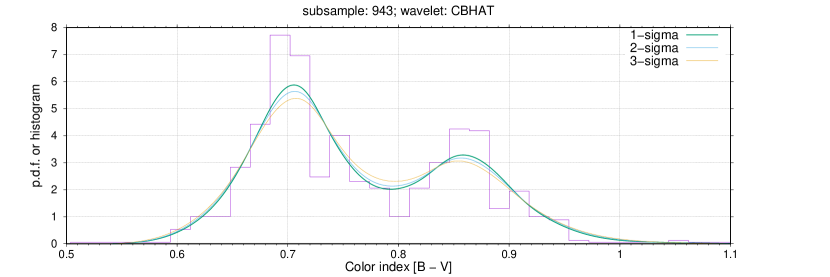
Figure 4: Wavelet analysis for the distribution of asteroids color index $B-V$, CBHAT.

The color index $B-V$ appeared more interesting, shown in Fig. 4. It reveals a bimodality with a clear gap between two modes, near $0.71$ and $0.86$. The larger peak is likely related to carbonaceous asteroids, while the smaller peak contains rocky asteroids.

These distributions of physical parameters appeared quite simple. We were able to resolve only the large-scale patterns that could be easily seen in histograms. The wavelet analysis only confirmed that there are no detectable small-scale details.

5.2 Distributions of proper orbital elements

Finally, we proceed to the proper orbital elements. Now we consider the same three orbital parameters $e$, $i$ and $a$, as in the osculating case.

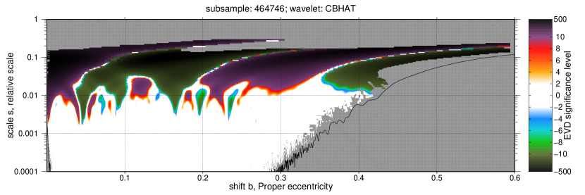
Figure 5: Wavelet analysis for the distribution of asteroids proper orbital eccentricity $e_{p}$, CBHAT.

As we can see from Fig. 5, the distribution of proper eccentricities demonstrates multiple local inhomogeneities. Those inhomogeneities are likely related to various asteroid families. For example, the density concentration for $e_{p}$ in the range $0.045-0.05$ is possibly related to the Hoffmeister and Astrid families, the range $0.19-0.2$ is related to Dora family (see Table LABEL:AstDysFamilies). However it is not easy to set a one-to-one correspondence between families from Table LABEL:AstDysFamilies and peaks of the 1D distribution of $e_{p}$. This is probably because multiple families overlap with each other in such 1D view.

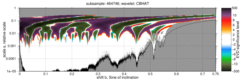
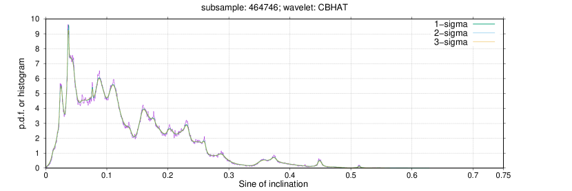
Figure 6: Wavelet analysis for the distribution of asteroids proper inclination $i_{p}$, CBHAT.

The proper orbital inclination (Fig. 6) reveals qualitatively similar behaviour. At least $15$ local concentrations can be detected, which can be related to the asteroid families, or some dynamical effects. However, it is again difficult to unambiguously separate these families from each other based on just the 1D analysis.

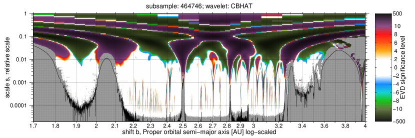
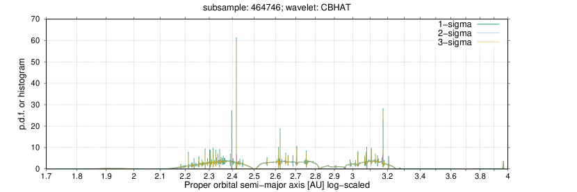
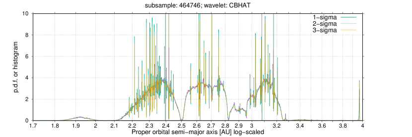
Figure 7: Wavelet analysis for the distribution of asteroids proper semimajor axis $a_{p}$, CBHAT. The second p.d.f. plot has a cutted ordinate to show the most informative portion of the graph.

The distribution of the proper semimajor axis (Fig. 7) appears the most informative and the most interesting among all other 1D distributions. The thin resonant bands (gaps as well as concentrations) are detected very easily. However, such extremely narrow groups are mainly associated to just the mean-motion resonaces affecting the motion of the asteroids. They are not related to the “asteroid families” in the genetic sense of this notion. We revealed $110$ such resonant asteroid groups, they are given in Table LABEL:ResonantFamilies. In the first column we show the number of the brightest asteroid of a group (or the smallest absolute magnitude).

Notice that although we attribute them to resonances here, and some of them indeed have obvious commensurability with e.g. Jupiter, we did not formally verify that the resonant dynamics indeed takes place.

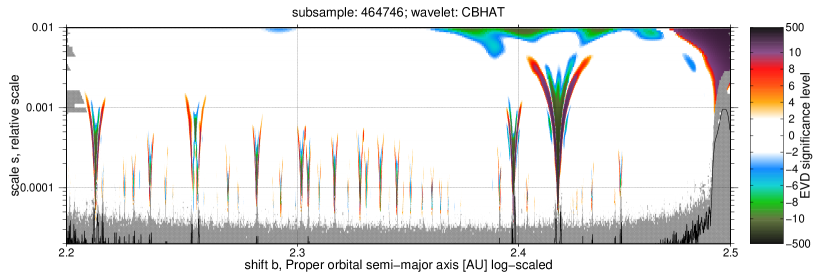
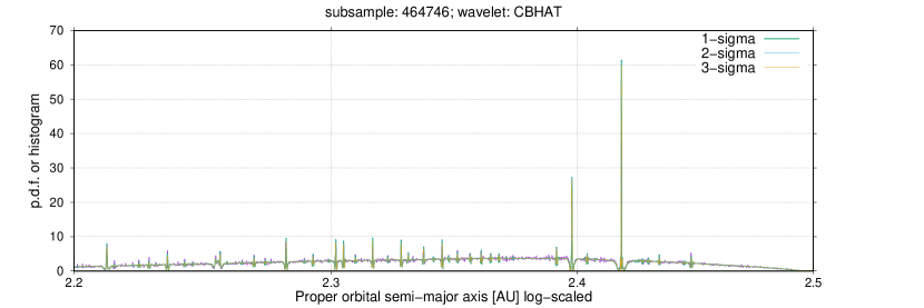
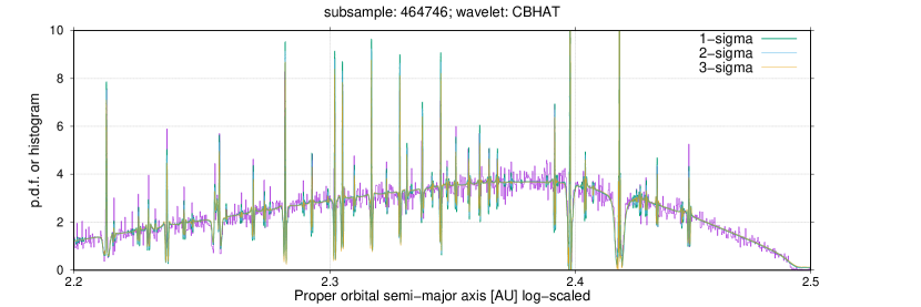
Figure 8: Wavelet analysis for the distribution of asteroids proper semimajor axis $A_{p}$, range $2.2-2.5$ AU, CBHAT. The second p.d.f. plot has a cutted ordinate to show the most informative portion of the graph.

For a more clear presentation we also plot in Fig. 8 an expanded small portion of Fig. 7 in the cutted range $2.2-2.5$ AU.

In addition we may notice that our 1D analysis is capable to easily resolve the internal structure of the resonant families, and this fine structure appears rather intricate. Each such family has an extremely thin core surrounded by two wider gaps from the both sides. Moreover, the shape of the core appears very peaky, relatively to e.g. the Gaussian bell shape. This might be interrelated with some properties of resonant motion, or with artifacts of the averaging procedure used to derive proper semimajor axis.

Table 2: Resonant asteroid families detected by the 1D analysis.

Core	$N$	$a_{\min}$	$a_{\max}$		Core	$N$	$a_{\min}$	$a_{\max}$
9900	203	2.141	2.144		1145	539	2.424	2.425
3972	180	2.163	2.164		6	330	2.4252	2.4258
2770	192	2.1695	2.1705		1108	382	2.427	2.4277
1468	381	2.1815	2.183		585	482	2.4293	2.4302
512	253	2.1885	2.1895		112	543	2.4338	2.4348
1733	254	2.193	2.194		79	273	2.4441	2.4447
270	279	2.198	2.199		4088	190	2.4449	2.4453
8	280	2.201	2.202		2026	221	2.4455	2.446
43	168	2.2032	2.2037		138	456	2.4472	2.4482
1219	1011	2.2105	2.213		13698	217	2.4485	2.449
443	311	2.215	2.216		2898	267	2.556	2.5565
1123	399	2.2245	2.2255		1658	510	2.5595	2.5603
422	578	2.228	2.2295		429	640	2.607	2.608
937	388	2.231	2.232		70	811	2.6145	2.6155
685	511	2.2355	2.2365		53	812	2.618	2.619
1523	411	2.242	2.243		792	1069	2.6225	2.6235
2037	239	2.2455	2.246		615	616	2.6305	2.6315
822	1524	2.254	2.257		476	2505	2.649	2.653
3982	486	2.2585	2.2595		102	638	2.661	2.662
1899	493	2.2645	2.2655		64	417	2.6811	2.6818
1078	503	2.269	2.27		166	596	2.6855	2.6865
3841	510	2.2735	2.2745		868	1631	2.704	2.706
5764	288	2.276	2.2765		1904	396	2.7433	2.744
548	624	2.282	2.2825		934	367	2.7478	2.7485
2013	434	2.2893	2.29		485	1567	2.751	2.753
1419	470	2.2925	2.2932		356	454	2.7565	2.7573
45153	320	2.299	2.2995		143	562	2.761	2.762
4262	769	2.3015	2.3025		446	441	2.787	2.7878
6189	676	2.3045	2.3055		1092	1306	2.901	2.909
1982	403	2.3095	2.31		22	226	2.909	2.91
1959	749	2.316	2.317		677	241	2.9555	2.9575
4408	639	2.322	2.323		447	506	2.9855	2.9863
1083	680	2.3277	2.3285		117	346	2.991	2.992
2762	551	2.3305	2.3312		221	381	3.012	3.013
1664	385	2.3325	2.333		478	539	3.0155	3.017
290	666	2.3368	2.3375		592	3431	3.0208	3.03
9963	729	2.341	2.342		1488	334	3.0385	3.0391
1367	794	2.344	2.345		4410	617	3.054	3.0552
27	736	2.347	2.348		368	578	3.067	3.068
3895	597	2.3505	2.3512		202	3354	3.074	3.078
4857	527	2.3558	2.3565		2395	460	3.0795	3.082
1646	773	2.36	2.361		1684	343	3.0908	3.0913
916	723	2.364	2.365		86	1910	3.105	3.1072
163	753	2.367	2.368		196	648	3.1135	3.1145
1573	466	2.3703	2.371		382	743	3.122	3.1232
584	719	2.373	2.374		375	1531	3.128	3.1302
249	437	2.3772	2.3778		10	770	3.141	3.1422
4904	780	2.388	2.389		209	677	3.147	3.1485
1591	874	2.3908	2.392		2494	583	3.16	3.161
1077	565	2.3921	2.3929		1023	1105	3.167	3.169
463	1416	2.397	2.3983		511	2761	3.173	3.1752
304	1363	2.403	2.405		778	500	3.18	3.181
4132	320	2.407	2.4075		530	1048	3.2065	3.2088
6334	331	2.4075	2.408		1362	316	3.273	3.277
182	2724	2.4178	2.4192		190	1986	3.956	3.9687

6 Bivariate distributions and 3D analysis via 2D projections

The 2D wavelet analysis appears more complicated, because the 2D geometry is considerably more diverse than the 1D one. Also, the 2D case is more computationally demanding. In (Baluev et al, 2020a) the 2D wavelet analysis algorithm is presented, based on the optimised radially-symmetric (isotropic) wavelets 2DOPT_1,2. These two wavelets are almost identical, and here we use the 2DOPT₂ version which we refer to as just 2DOPT for simplicity.

Regardless to the complications, the 2D analysis appears analogous to 1D one in many aspects. However, because of the isotropic restriction on the wavelet shape, this algorithm can be only applied to physically comparable (summable) parameters, and targets mainly patterns that have similar size in the both directions.

The 1D analysis above was focused on the following orbital parameters: eccentricity $e$, inclination $i$, and semimajor axis $a$. We have not constructed a 3D algorithm yet to process this 3D space $(a,e,i)$ in a self-consistent manner, but we can consider three independent 2D subspaces: $(a,e)$, $(a,i)$, and $(e,i)$. We may consider a 2D density in each of these planes and investigate it using our 2D algorithm.

We adopt the following system of comparable parameters: $(\log a,e,\sin i)$. Here, $\log a$ appears instead of $a$ because the differences like $\Delta\log a\simeq\Delta a/a$ appear adimensional, as well as the differences $\Delta e$ or $\Delta\sin i$. Hence, we can legally compare various small ranges in terms of $\log a$ with ranges for $e$ and $\sin i$ (hence, all three wavelet scales appear dimensionless). Concerning the physical comparability of $e$ and $\sin i$, it follows because these (or equivalent) parameters often play equal roles in various dynamical equations; this is highlighted by e.g. the Lidov-Kozai mechanism where these parameters can “flow” one into another through the conservation of the quantity $\sqrt{1-e^{2}}\cos i$, so $e$ can be exchanged with $\sin i$ (Murray and Dermott, 1999, chap. 7).

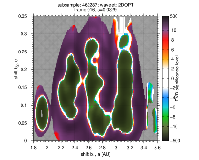
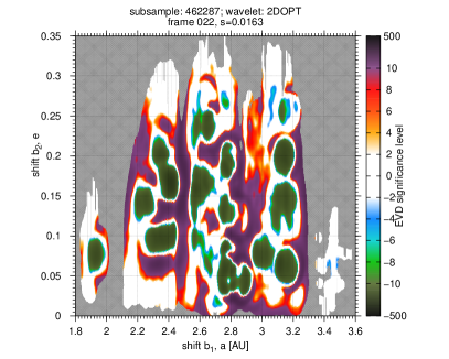
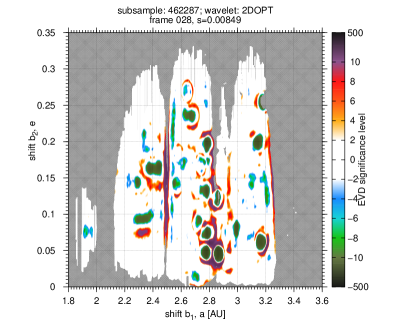
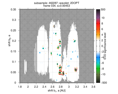
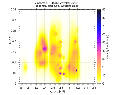
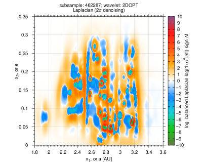
Figure 9: Top quadruplet: $4$ frames of the 2D wavelet transform for the $(\log A,e)$ bivariate distribution (proper elements). The animation containing the full CWT evolution is also attached as online-only material. Bottom pair: p.d.f. model reconstructed by matching pursuit iterations and its Laplacian.

For example, let us consider the $(\log a,e)$ pair (Fig. 9). Notice that the wavelet transform is a function of three variables now, so we plot several frames corresponding to difference scales. Each such frame is plotted as a significance map (as in the 1D analysis).

However, investigating the 2D wavelet transform directly does not appear very easy, since we should treat multiple resolution levels simultaneously. The reconstructed p.d.f. model would be more helpful here, because it joins all resolution levels into the same plot, simultaneously keeping only the significant detected structures. However, in practice the p.d.f. graphs appeared too much diffuse and inconclusive, because they do not highlight subtle asteroid families even if they are statistically significant. Such a subtle cluster would appear almost indistinguishable over the large-scale background, because it changes the background level only very slightly. We found that this issue can be solved by considering the Laplacian of the p.d.f. model rather than this model itself. This is justified by the known property that the CWT represents a smoothed Laplacian (Baluev et al, 2020a), so in fact our wavelet analysis deals with the p.d.f. Laplacian rather than p.d.f. itself. The Laplacian can be easily computed by applying the CWT with a small scale (smaller than scales of all the detected structures).

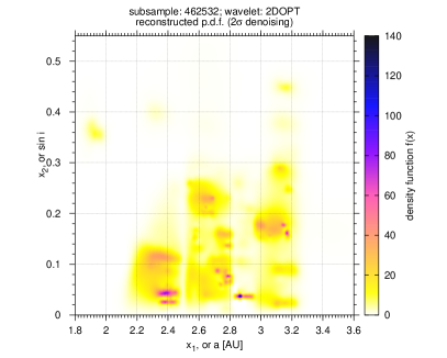
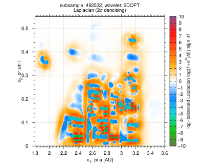
Figure 10: The reconstructed p.d.f. model for the $(\log a,\sin i)$ bivariate distribution and its Laplacian.

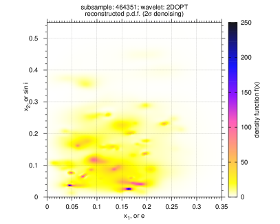
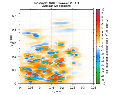
Figure 11: The reconstructed p.d.f. model for the $(e,\sin i)$ bivariate distribution and its Laplacian.

As we can see, the Laplacian appears very helpful to visually spot even very subtle families in any of the bivariate distributions that we considered (Fig. 9, 10, 11). To further highlight the color contrast, we plot here a logarithmically-modified quantity $\log(1+\sigma^{4}|\Delta f|)\mathop{\mathrm{sign}}\nolimits\Delta f$, where $\sigma^{2}=\sigma_{1}^{2}+\sigma_{2}^{2}$ is the cumulative variance of the two random variables.

We can see that boundaries of a cluster can be determined as boundaries of an isolated domain (“spot”). Notice that it is important to pay attention to an opposite-sign ring around each spot. If it is present then we have a local convexity (negative Laplacian) surrounded by a concavity ring (positive Laplacian). Such a structure can be interpreted as an isolated cluster. However, if this ring is not present (not significant) then we cannot claim that such a geometric structure is a family, because it is not separated from the background. We adopt this rule as a basic formalized definition of a “cluster” in this work. This treatment is justified in more details in a separate work devoted to the stellar population analysis (Baluev et al, 2020b).

A more difficult question appears if some hints of a ring are present, but the ring is incomplete, or if there are two partly merged 2D spots not separated from each other by a zone of positive Laplacian. This typically appears in case of overlapping families. Since such families can often be distinguished with the help of the third parameter (the one not involved in the given 2D plot), we investigate each such case individually.

We try to understand the 3D p.d.f. via its 2D projections, so the overlapping effect becomes very important. For each potential family (or a group of overlapping families) in each of the three 2D diagrams we cut out a rectangular box in the corresponding 2D plane and consider the subsample containing only asteroids within this box. For each such subsample we performed a 1D wavelet analysis of the third parameter and constructed the corresponding 1D p.d.f. containing only statistically significant patterns. Such 1D distributions suggest useful hints allowing to resolve various ambiguities concerning family overlapping. For example, if this distribution is unimodal then the given candidate family is homogeneous (no overlapping). If there are additional modes then the apparent 2D family actually contains two overlapping families corresponding to different values of the third parameter, and so on. These hints can be additionally verified by looking at the other two 2D planes.

Of course, there are more difficult cases that cannot be resolved unambiguously based on just the 2D projections. This may occur in case of a partial overlap of multiple families in all 2D diagrams and other nuisance effects (Baluev et al, 2020a). Nevertheless, we found $44$ asteroid families that can be resolved clearly. They are listed in Table LABEL:residual. The families were cross-identified with the known AstDys ones (Table LABEL:AstDysFamilies) by comparing their boundaries. We find that almost every of our wavelet-detected family has and HCM-based counterpart, but the wavelet-derived ranges are systematically more narrow. Notice that the boundaries of a family can be rather diffuse and thus their exact position is largely a matter of convention. Our convention is to define the boundary based on zero Laplacian (or zero second derivative in the 1D distribution). Our results suggests that this convention leads to a more restrictive boundaries than from HCM, this is the same effect as in (Baluev et al, 2020b).

Table 3: Asteroid families detected on the basis of 2D wavelet analysis.

No	HCM core	$a_{\min}$	$a_{\max}$	$e_{\min}$	$e_{\max}$	$\sin i_{\min}$	$\sin i_{\max}$
W1	434	1.87	1.99	0.057	0.094	0.345	0.380
W2	2076	2.265	2.31	0.138	0.150	0.088	0.102
W3	4	2.25	2.48	0.083	0.129	0.105	0.126
W4	163	2.32	2.37	0.199	0.217	0.08	0.096
W5	27 (FIN410)	2.34	2.4	0.179	0.201	0.008	0.014
W6	20	2.345	2.465	0.149	0.171	0.022	0.029
W7	5026	2.37	2.41	0.199	0.217	0.079	0.093
W8	302	2.385	2.405	0.103	0.112	0.055	0.063
W9	1658	2.53	2.645	0.164	0.179	0.125	0.138
W10	3815	2.555	2.585	0.136	0.144	0.143	0.161
W11	606	2.57	2.595	0.175	0.184	0.162	0.171
W12	3	2.6	2.70	0.227	0.245	0.226	0.237
W13	145	2.6	2.705	0.155	0.178	0.196	0.208
W14	1547	2.635	2.655	0.261	0.276	0.209	0.215
W15	808	2.705	2.735	0.13	0.139	0.082	0.092
W16	3827	2.705	2.74	0.083	0.094	0.082	0.092
W17	173 (FIN522)	2.715	2.745	0.171	0.183	0.227	0.238
W18	396	2.725	2.75	0.164	0.172	0.056	0.064
W19	668	2.74	2.81	0.19	0.202	0.131	0.141
W20	93	2.745	2.815	0.122	0.14	0.151	0.17
W21	847	2.75	2.79	0.067	0.076	0.06	0.069
W22	808	2.75	2.81	0.128	0.139	0.082	0.093
W23	1128	2.75	2.815	0.044	0.053	0.006	0.018
W24	2353	2.76	2.81	0.087	0.103	0.08	0.093
W25	18466	2.76	2.81	0.171	0.181	0.227	0.238
W26	1726	2.77	2.815	0.044	0.053	0.073	0.079
W27	847	2.79	2.815	0.067	0.082	0.06	0.076
W28	158	2.83	2.85	0.043	0.055	0.033	0.04
W29	293	2.83	2.89	0.116	0.128	0.254	0.265
W30	158	2.84	2.865	0.063	0.072	0.033	0.04
W31	158	2.85	2.88	0.04	0.049	0.033	0.04
W32	16286	2.85	2.88	0.04	0.049	0.093	0.115
W33	845	2.89	2.96	0.026	0.047	0.202	0.214
W34	158	2.91	2.945	0.062	0.089	0.032	0.04
W35	221	2.96	3.025	0.070	0.093	0.163	0.187
W36	179	2.975	3.01	0.061	0.07	0.149	0.153
W37	96	3.03	3.065	0.179	0.191	0.275	0.288
W38	283	3.04	3.07	0.107	0.120	0.153	0.16
W39	24	3.07	3.12	0.138	0.156	0.016	0.029
W40	1040	3.105	3.165	0.189	0.207	0.280	0.295
W41	3330	3.13	3.17	0.189	0.207	0.173	0.181
W42	24	3.14	3.17	0.147	0.157	0.017	0.028
W43	778	3.145	3.205	0.246	0.264	0.240	0.255
W44	490	3.155	3.18	0.057	0.066	0.157	0.167

We notice that our wavelet analysis detected three asteroid families not mentioned in AstDys (W5, W17, W24). After a closer look, it appeared that W5 and W17 are the 27 Euterpe and 173 Ino families mentioned by Nesvorný et al (2015) as FIN410 and FIN522. However, there is no more details about these families, and they are not included in AstDys. The corresponding asteroids are labelled in AstDys as not involved in any family. Therefore, we see some controversy in the literature concerning these two families, and our analysis resolves it positively. The third family W24 has the smallest-number asteroid 2353, and likely appears unknown.

Simultaneously, there are many HCM-based families not detected by wavelets. In some part, this can be explained by the overlapping effect which disabled unambiguous detection of some families by wavelets. Likely, the full 3D wavelet analysis would detect more families, but we currently do not have a working 3D extension of our wavelet analysis pipeline (this needs substantial additional theory work and computing optimisations). However, the overlapping does not explain all such occurrences well. Many of the HCM-only families just do not reveal themselves in our wavelet analysis, that is they appear statistically insignificant in our approach. From the other side, some of them may appear more significant in the full 3D analysis. But at the current stage such families are possibly more doubtful and require additional investigation that falls out of the scope of the present paper.

Also, we notice that some HCM-detected families may reveal a complicated structure. In our analysis they are split into multiple subfamilies (up to $4$, like the Koronis family). In some part this may indicate that our wavelet analysis tends to generate some crowding effect, contrary to the HCM chaining.

Concerning the resonant asteroid families, we did not detect them in the 2D analysis, likely because they should reveal themselves as extremely elongated thin patterns. Notice that our 2D analysis is based on isotropic radially-symmetric wavelets, so it is expectedly insensitive to such disproportional structures.

7 Conclusions and discussion

Our main conclusion is that statistical wavelet analysis appears as a useful alternative tool allowing to independently verify the HCM results. Let us now review their main differences and outline sevelar prospects to advance futher.

1. The wavelets generate a crowding effect opposite to the HCM chaining effect (as expected). This results in a fragmentation of large statistical clusters into smaller subgroups. One reason for such a difference is that we use radially symmetric wavelets that naturally tends to decompose an elongated structure into a sequence of more or less oval ones.

2. In the framework of the wavelet analysis, the balance between the crowding and chaining effects can be controlled through the use of non-radially-symmetric elliptically distorted wavelets. Currently such wavelets are not used at all, but it is possible to include them by replacing a single scale parameter $s$ with a general scale matrix in (1). In such a case elongated and radially symmetric wavelets can be combined together using a tunable weight function (to appear in (2)). Increasing the role of elliptic wavelets would bias the method to have more chaining effect. However, the use of elliptic wavelets implies a jump of dimensionality and hence the need to rework the entire computing approach (see below).

3. Both the methods, wavelets and HCM, involve some dependence on various assumptions. While HCM may depend on the metric used, the wavelet analysis depends on the wavelet shape. Moreover, selecting different wavelets we may control the underlying metric. For example, radially symmetric wavelets imply the use of a local $L_{2}$ metric in the space of the variables that we analyse. In our wavelet algorithm the radial symmetry is also a just a particular prior assumption, but beyond this restriction the wavelet radial function $\psi(t)$ was derived from certain optimality criteria to minimize the noise (and to increase the S/N ratio for possible patterns). In view of this, it might be an interesting idea trying to find some optimal metric for HCM.

4. Our wavelet analysis is currently limited by two dimensions, while both the asteroid families search presented here and stellar population analysis presented in (Baluev et al, 2020b) assume at least 3D spaces. The generalization of the wavelet analysis and the associated tools to $\mathbb{R}^{n}$ with $n>2$ is not difficult mathematically, but it infers significant increase of computational issues. The computing approaches of our algorithm should be reworked qualitatively then. The main issues are the efficient discrete coverage of the shift-scale space for 1 and numeric integration of (2). Currently this is achieved through a regular rectangular grid, but results in exponential dependence of the required resources on the dimensionality.

5. We found considerably smaller number of asteroid families than known from the HCM method. It looks as if many HCM families have too low statistical significance in our analysis and look like just noise. However, we are unsure about this conclusion because similar effect can appear by other reasons. In some part it can be explained by law dimensionality of our analysis (e.g. a statistical group can appear more dense in some additional variable that we did not consider here). In some part this appeared due to overlapping effect (we could not disentangle all 3D asteroid families based on 2D projections). So this issue requires further investigation.

6. In addition to all said above, our analysis allowed to reveal some new families not detected with HCM, to confirm possibly controversial families, and to reveal internal structure in big HCM families.

7. The wavelet analysis is not a cluster detection tool in the strict meaning of this term, so it does not classify particular objects. Therefore, it does not provide information which particular object should be included to a family and which is not (in particular, whether a particular object belongs to a particular cluster or is from the background). The purpuse of the wavelet analysis is to analyse the statistical distribution as a smooth function and to detect unusual patterns inside it.

Therefore, we may argue that the wavelet analysis was undeservedly abandoned in this task over years. It can be used as an independent method of cluster detection, in particular in the asteroid families search, but it also needs further development.