Object Detection for Remote Sensing Images Based on Polar Coordinates

Abstract

Arbitrary-oriented object detection is an important task in the field of remote sensing object detection. Existing studies have shown that the polar coordinate system has obvious advantages in dealing with the problem of rotating object modeling, that is, using fewer parameters to achieve more accurate rotating object detection. However, present state-of-the-art detectors based on deep learning are all modeled in Cartesian coordinates. In this article, we introduce the polar coordinate system to the deep learning detector for the first time, and propose an anchor free Polar Remote Sensing Object Detector (P-RSDet), which can achieve competitive detection accuracy via uses simpler object representation model and less regression parameters. In P-RSDet method, arbitrary-oriented object detection can be achieved by predicting the center point and regressing one polar radius and two polar angles. Besides, in order to express the geometric constraint relationship between the polar radius and the polar angle, a Polar Ring Area Loss function is proposed to improve the prediction accuracy of the corner position. Experiments on DOTA, UCAS-AOD and NWPU VHR-10 datasets show that our P-RSDet achieves state-of-the-art performances with simpler model and less regression parameters.

=-15pt

I Introduction

In recent years, oriented object detection in remote sensing images has attracted increasing attention. Detection performance has made extraordinary progress driven by the applications of deep convolution neural network (DCNN). Present DCNN-based detectors in the remote sensing field can be divided into two research branches according to the different output forms: horizontal and oriented bounding box. And these two types of models have their own advantages in practical application.

Most horizontal detectors[1, 2, 3, 4] are designed based on anchor mechanism which is first proposed in Faster RCNN [5]. They set up anchor boxes with different sizes and aspect ratios intensively in feature maps to guide the regressions of the position as well as the size of each object. This type of detectors in remote sensing are easy to design and simple to implement relatively, and sometimes can obtain satisfactory results without nearly any changes in the original baselines [5, 6, 7, 8, 9, 10, 11]. However, it is imprecise to locate objects which have large aspect ratios with the output form of a horizontal bounding box. As shown in Figure 1(a), when the aspect ratio of an object is large, the horizontal bounding box will bring a lot of redundant pixels that do not belong to the object, which will make the final locating results inaccurate. In addition, in the anchor-based network, when two large aspect ratio objects park side by side, their horizontal bounding boxes may have a large Intersection over Union(IOU), which will cause one of them to be filtered out by Non Maximum Suppression(NMS) resulting in missed detection.

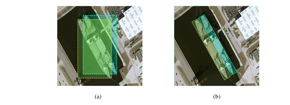
Figure 1: When the aspect ratio of an object (such as warship) is large, the horizontal bounding box is not a good representation of object as shown in Figure (a). At present, oriented bounding box as shown in Figure (b) becomes more popular, beacause its location is more accurate

The problems faced with horizontal detectors aforementioned can be solved by oriented detectors[12, 13, 14, 15, 16, 17]. As shown in Fig. 1(b), the output form of this type of detector is oriented bounding box which can provide a more precise location for the object with large aspect ratio. However, the design of these models is more complicated than that of horizontal ones. In order to achieve the aim of getting the oriented bounding box, J. Ma et al.[12] design Rotated Region Proposal Network(RRPN) in which more anchors with different angles will be set. In addition, both the IoU and NMS in horizontal models should be replaced by more complex ones with oriented form. Although this kind of anchor-based detectors are effective in the detection of specific objects, the cost of devising them is usually large.

Moreover, all the above methods have one characteristic in common: objects are modeled based on the Cartesian coordinate system. The Cartesian coordinate system has advantages in presenting the horizontal bounding box, because only width and height are needed when the center point is known as shown in Fig. 2(b). However, in Cartesian coordinate system, the oriented object is usually represented by five-parameter ($x,y,w,h$, $\theta$) or eight-parameter ($x_{1},y_{1},x_{2},y_{2},x_{3},y_{3},x_{4},y_{4}$) as shown in Fig. 2(d), which are complex. We note that when a bounding box revolves around its center point, the trajectory of its four corner points is exactly a circle. Referring to this kind of rotation and circular problem, polar coordinate system is a better choice compared with Cartesian coordinates.

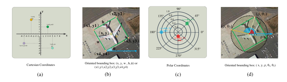
Figure 2: Oriented bounding box representations in Cartesian and Polar coordinates. In Cartesian coordinate system, the oriented bounding box representations are usually $(x,y,w,h,\theta)$ or $(x_{1},y_{1},x_{2},y_{2},x_{3},y_{3},x_{4},y_{4})$ as shown in (b). In polar coordinates, a point can be represented by $(\rho,\theta)$, where r is the polar radius and q is the polar angle. When the center point is taken as the pole point of polar coordinates, oriented bounding box can be represented by $(x,y,\rho)$ as shown in (d).

Figure 3: The illustration of the detection pipeline. (a) Previous detectors usually adopts anchor-based mechanism, that is, regressing angle, width, height, center point position and category probability based on proposals. (b) Our P-RSDet adopts anchor free mechanisam. It realizes pole points localization and classification simultaneously in the process of pole points extracting, and realizes regression of polar angle and radius in regression process.

In this paper, a new model named Polar Remote Sensing Object Detector (P-RSDet) based on polar coordinate system is proposed. P-RSDet abandons two inherent modes of most present remote sensing detectors: anchor-based and Cartesian coordinates modeling. Previous detectors usually adopts anchor-based mechanism, that is, regressing angle, width, height, center point position and category probability based on proposals as shown in Fig.3(a). Instead, P-RSDet performs object detection in polar coordinates and an anchor-free manner. As shown in Fig. 2(d), if the center point of bounding box is taken as the pole point and the horizontal-right direction is taken as the polar axis, arbitrary oriented bounding box can be denoted by one polar radius and two polar angles with the form of ($\rho$, $\theta_{1}$, $\theta_{2}$). In order to realize the above detection method, P-RSDet outputs four maps of which one is a heatmap to predict the locations of pole points in keypoint detection way and the other three are used to regress polar radius $\rho$ and polar angles $\theta_{1}$, $\theta_{2}$ respectively. As illustrated in Fig. 3(b), P-RSDet is also and end-to-end model. It realizes pole points localization and classification simultaneously in the process of pole points extracting, and realizes regression of polar angle and radius in regression process. It combines polar coordinates with anchor free to realize arbitrary-oriented object detection in a simple way. In addition, P-RSDet achieves satisfactory results on multiple remote sensing public datasets, which proves its excellent performance.

Above all, our innovations and contributions are as follows:

(1). We propose an anchor free detection model based on polar coordinate system named Polar Remote Sensing Object Detector (P-RSDet). Compared with other deep learning-based detection methods based on Cartesian coordinates, our method achieves competitive accuracy with simpler model and less regression parameters.

(2). In order to solve the problem that Smooth-L1 loss ignores the geometric correlation between points, we propose an additional novel loss function Polar Ring Area Loss for more accurate predicted bounding box. The Polar-Ring-Area Loss function increases the correlation between polar radius and polar angle, and avoids the regression inaccuracy caused by neglecting their geometric correlation.

(3). Considering that the remote sensing objects are numerous, the top K center points extracting technique used in nature scenes will lead to missing detection. For this problem, we propose a new technique that extracting extreme points from heatmap as center points to reduce the rate of missing detection.

The rest of this paper is organized as follows: We briefly review the representative related works and basic principle in our method in Section II. The details of P-RSDet are shown in Section III. The experiment results and analyses are shown in Section IV. At last, our work is summarized and concluded in Section V.

II Related Works

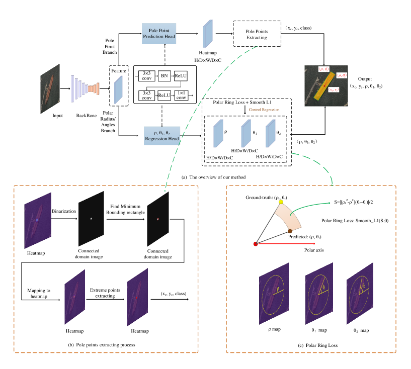
Figure 4: Architecture of P-RSDet. (a) The overview of our P-RSDet. When an image inputs our model, it will output four maps in parallel. One is the heatmap which used to predict the pole point, and the other three are used to regress $\rho$, $\theta_{1}$, $\theta_{2}$ respectively. Therefore, we need to regress four parameters in all, i.e. $(p,\rho,\theta_{1},\theta_{2})$ represents the probability that a point in the heatmap is the pole point. These 4 maps have $c$ channels which represent $c$ classes. (b) The detailed process of pole point extracting. (c) The diagram of Polar Ring Loss definition.

II-A Oriented Object Detection

With the development of deep learning, oriented object detection has made great process. Many oriented object detetion algorithms are improved based on horizontal detection algorithms.

Horizontal object detection algorithms can be divided into two types: anchor-based models[5][9][11][24, 25, 26, 27, 28] and anchor-free models[18, 19, 20, 21, 22] according to whether the anchor mechanism is used. Anchor-based models represented by Faster RCNN[5] need to set up a series of anchor boxes, which can be regarded as fixed reference regions with different scales and ratios. Anchor free models can be roughly divided into keypoint based models which are represented by CornerNet[19] and per-pixel detection models which are represented by FCOS[22].

For oriented detection models, they can also be divided into anchor-based models and anchor-free models. In the filed of text detection, there are some anchor-based oriented object detection algorithms that are worth learning. RRPN[12] and R2CNN[13] based on Faster RCNN are two of them. R$2$CNN adds two pooled sizes and a branch to regress inclined box coordinates. RRPN improves RPN in Faster RCNN by adding rotation anchors with different angles. In addition, P. Lyu et al. [29] combine corner points detection and text region segmentation to realize oriented scene text detection. In [29], after detecting corner points with default boxes, candidate bounding boxes are generated by sampling and grouping these corner points. Finally, position-sensitive segmentation maps are used to score the candidate bounding box. In the field of remote sensing, R-DFPN[14] improves [12] to obtain a precise oriented bounding box to solve the problem of ship rotation and dense parking. Different from [12] and [14], Ding et al.[30] propose a Region of Interest(RoI) Transformer which transforms a horizontal RoI into rotated RoI to obtain rotated region proposals. However, these anchor-based oriented detectors not only face the disadvantages brought by anchor, but also greatly increase the computation complexity of the whole network.

Benefited from the simplicity and flexibility, anchor-free horizontal object detectors have also been improved to realize oriented object detection. Wei et al. [16] abandons anchor mechanism to avoid the complexity of the anchor design. Nevertheless, it needs regressing eight offsets, which leads to too many degrees of freedom and requires more complex loss functions to control them. Our P-RSDet, which directly models objects in the polar coordinate system and only needs to regress four parameters, pursues detecting oriented objects in a simple yet efficient way.

II-B Polar Coordinates

Polar cooridinates are widely used in many fileds[31, 32, 33, 34, 35]. Gai et al.[31] propose a calibration method based on polar coordinate. This paper shows that the relationship in polar coordinates image is relatively simple, thus the complexity of the calibration is simplified. B Gergič et al.[33] compare between SAR data compression in Cartesian and polar coordinates. They prove that the compression of complex SAR data in polar coordinates has smaller amplitude and phase errors than in Cartesian coordinates.

In traditional remote sensing object detection algorithms which are not based on deep learning, polar coordinates are also used to solve some problems. Wang et al.[34] divide the geospatial objects with complex shape into several main parts, and the structure information among parts is described and regulated in polar coordinates to achieve the rotation invariance on configuration. Wang et al.[35] use the polar angle of each pixel to normalize the its gradient direction, and generate the histograms of oriented gradients according to the new directions to steer the rotation problem.

It can be seen that polar coordinates have advantages in rotation and direction related problem. Reasonable use of polar coordinates can simplify the object modeling and reduce the complexity of the model.

III P-RSDet

First, in this section, the framework of the proposed P-RSDet is briefly introduced. Then, boundary problem is described in detail. Third, we show how the oriented objects in remote sensing images are modeled based on polar coordinates. Finally, we elaborate the details of our model, including the design of specific loss functions and the optimization of keypoints extraction method.

III-A Framework

Figure 4 illustrates the overall framework of our P-RSDet. A modified higher-resolution ResNet-101[21] with $4$ output stride is selected as the Encoder-Decoder of P-RSDet. Suppose the size of one input image is $W\times H$, P-RSDet will output four maps with $C\times\frac{W}{d}\times\frac{H}{d}$ size, where $C$ is the number of categories and $d$ represents the output stride which is $4$ as aforementioned. In these four output maps, one is in the form of heatmap to predict the pole points, and the other three are to regress the corresponding polar radius and the polar angles of each object. As mentioned above and shown in Fig. 4, our model is very simple to design.

III-B Objects in Polar Coordinates

The four corner points of the oriented bounding box are usually represented by ($x_{1}$, $y_{1}$), ($x_{2}$, $y_{2}$), ($x_{3}$, $y_{3}$), ($x_{4}$, $y_{4}$) in Cartesian coordinates. In order to model it in polar coordinates, for an object, we first make its center point be the pole point of polar coordinate system, then the horizontal-right direction and the counterclockwise are taken as the positive direction of the polar axis and polar angle in radians respectively. In this coordinate system, the four corners can be represented in sequence as ($\rho_{1}$, $\theta_{1}$), ($\rho_{2}$, $\theta_{2}$), ($\rho_{3}$, $\theta_{3}$), ($\rho_{4}$, $\theta_{4}$).According to the properties of rectangle, we can get the following relations:

$$\rho_{1}=\rho_{2}=\rho_{3}=\rho_{4}$$ (1)

$$\theta_{3}=\theta_{1}+\pi,\theta_{4}=\theta_{2}+\pi$$ (2)

Therefore, let $\rho=\rho_{1}=\rho_{2}=\rho_{3}=\rho_{4}$, only three variables, $\rho$, $\theta_{1}$ and $\theta_{2}$ are needed to represent a bounding box of object in Polar Coordinates.

In the inference phase, due to the process of evaluating the performance of one detector is only carried in Cartesian coordinates at present, we need to transform the point in polar coordinates to a Cartesian one. First, the positions of pole points ($x_{p}^{i}$, $y_{p}^{i}$) are extracted from heatmaps, where $i$ denotes the number of targets. Then according to the pole points, the polar radius and angles $\rho^{i}$, $\theta_{1}^{i}$ and $\theta_{2}^{i}$ are obtained from other three output maps. Finally, the final bounding boxes in the form of [($x^{i}_{1}$, $y^{i}_{1}$), ($x^{i}_{2}$, $y^{i}_{2}$), ($x^{i}_{3}$, $y^{i}_{3}$), ($x^{i}_{4}$, $y^{i}_{4}$)] can be obtained through the transformation calculation formulas as follows:

$$x_{n}^{i}=x_{p}^{i}+\rho^{i}\cdot\cos(\theta_{n}^{i})\quad y_{n}^{i}=y_{p}^{i}+\rho^{i}\cdot\sin(\theta_{n}^{i})$$ (3)

where $n$ represents $1,2,3$ and $4$.

III-C Pole Point Extraction

Accurate pole point prediction is very important for getting accurate bounding box. In our model, the detection of pole points follows CornerNet[19] for its excellent performance in the detection of keypoints of objects.

As mentioned in Section III-A, P-RSDet outputs a heatmap with size of $C\times\frac{W}{d}\times\frac{H}{d}$ for predicting pole points. The heatmap is actually a confidence map with the value $p\in[0,1]^{\frac{W}{d}\times\frac{H}{d}}$ of each pixel . In the training stage, let $h$ and $w$ represent the height and width of one bounding box, and the “ground-truth” of each point $(x,y)$ in the heatmap is given in form of Gauss kernel as $e^{-\frac{(x-x_{p})^{2}+(y-y_{p})^{2}}{2(min(h,w)/3)^{2}}}$, where $(x_{p},y_{p})$ is the equivalent points of the ground truth pole points after subsampling. A modified Focal Loss[10] follows CornerNet is used to guide the regression of pole points:

$$\mathcal{L}_{pole}\!=\!-\frac{1}{N}\!\sum_{cij}\!\begin{cases}\vspace{2 ex}(1-p_{cij})^{\alpha}log(p_{cij}),&\!p^{*}_{cij}=1\!\\ (1-p^{*}_{cij})^{\beta}(p_{cij})^{\alpha}\\ \quad log(1-p_{cij}),&\!p^{*}_{cij}=others\!\end{cases}$$ (4)

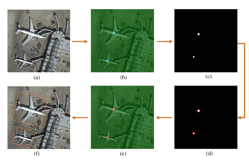
Figure 5: Process Flow Chart of pole point extraction. Figure (a) is the picture to be tested. Figure (b) is the heatmap generated by pole points detection branch. Figure (c) is the binary image converted from the heatmap. The red rectangles in Figure (d) represent the connected domains. Figure (e) shows the result of mapping the connected domains back to the original image. Figure (f) shows the final detection results after combining the other three regression branch results.

where $N$ is the number of objects in the input image, $\alpha$ and $\beta$ are the hyper-parameters which we set $\alpha$ to 2 and $\beta$ to 4 in experiments to control the contribution of positive and negative points. $p^{*}_{cij}$ is the “ground-truth” and $p_{cij}$ is the confidence with which a point at location $(i,j)$ be regarded as a pole point for class $c$ in the predicted heatmap.

We follow the method of keypoints detection in CornerNet during training stage. But in the test stage, the method of keypoint extraction in CornerNet is not suitable for us. Different from the natural images, a remote sensing image may contain hundreds of targets in the same class. CornerNet keeps $100$ keypoints with top scores, which may cause missed detection in remote sensing field.

Therefore, in P-RSDet, we optimize the extraction method. The overall process of pole point extraction is shown in Fig. 5. First, a threshold is set to convert the heatmap as shown in Fig. 5(b) into a binary images as shown in Fig. 5(c). Then, we find the connected domains in the binary image as shown in Fig. 5(d). Thirdly, the connected domains are mapped back to the heatmap and the peaks in these domains are taken as the predicted pole points.

III-D Polar Ring Area Loss

P-RSDet needs to regress polar radius $\rho$ and the first two angles $\theta_{1}$, $\theta_{2}$. For one bounding box, according to the original annotation $(x_{1}$, $y_{1})$, $(x_{2}$, $y_{2})$, $(x_{3}$, $y_{3})$, $(x_{4}$, $y_{4})$, let $(\sum_{i=1}^{4}x_{i}/4,\sum_{i=1}^{4}y_{i}/4$) be the pole point $(x_{p}$, $y_{p})$. Due to the error of mannual annotation, the distance between the four corners and the pole point are not necessarily equal, so the mean value of the four radii is taken as the target regression value of the polar radius. Therefore, the corresponding polar radius is computed as follows:

$$\rho=\frac{\sum_{i=1}^{4}[(x_{i}-x_{p})^{2}+(y_{i}-y_{p})^{2}]^{1/2}}{4}$$ (5)

For $\theta_{1}$ and $\theta_{2}$, we first compute the polar angles of four corners and turn them between 0 and $2\pi$, then choose the minimum two in the counterclockwise direction as $\theta_{1}$ and $\theta_{2}$. The angles are calculated as follows:

$$\theta_{i}\!=\!\left\{\begin{array}[]{lr}\!\pi/2,\quad x_{i}\!-\!x_{p}=0,y_{i}\!-\!y_{p}>0\\ \!-\pi/2,\quad x_{i}\!-\!x_{p}=0,y_{i}\!-\!y_{p}<0\\ \!arctan(\frac{y_{i}\!-\!y_{p}}{x_{i}\!-\!x_{p}}),\quad x_{i}\!-\!x_{p}>0,y_{i}\!-\!y_{p}\geq 0\\ \!\pi+arctan(\frac{y_{i}\!-\!y_{p}}{x_{i}\!-\!x_{p}}),\quad x_{i}\!-\!x_{p}<0,y_{i}\!-\!y_{p}\leq 0\\ \!\pi+arctan(\frac{y_{i}\!-\!y_{p}}{x_{i}\!-\!x_{p}}),\quad x_{i}\!-\!x_{p}<0,y_{i}\!-\!y_{p}<0\\ \!2\pi+arctan(\frac{y_{i}\!-\!y_{p}}{x_{i}\!-\!x_{p}}),\quad x_{i}\!-\!x_{p}>0,y_{i}\!-\!y_{p}<0\\ \end{array}\right.$$ (6)

So far, we have obtained all the regression targets, polar radius $\rho$ and the first two polar angles $\theta_{1},\theta_{2}$. Smooth-L1[36] Loss is selected to regress these three values in corresponding three output maps as follows:

$$L_{reg}^{{}^{\prime}}=\!\sum_{u=\rho,\theta_{1},\theta_{2}}\!Smooth\mathcal{L}1(u,u^{*})$$ (7)

In addition, considering the deviation between the predicted first two points with the ground-truth is determined by the radius error and the angle error together, we design a new loss named Polar Ring Area Loss for our model to control the above deviation.

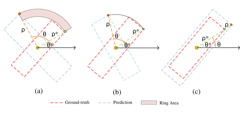
Figure 6: Ring Area in Polar Representation. $\rho^{*}$ and $\theta^{*}$ represent the ground truth of polar radius and angles. $\rho$ and $\theta$ represent the predicted polar radius and angles. Figure (a) shows that the predicted polar radius and angles all deviate from the ground truth. Figure (b) shows that predicted polar angles deviate from the ground truth but predicted polar radius is the same as the ground truth. Figure (c) shows that only the predicted polar radius deviates from the ground truth but predicted polar angles are the same as the ground truth.

As shown in Fig. 6, let $\rho,\theta$ be the prediction results and $\rho^{*},\theta^{*}$ be the ground-truth. As shown in Fig. 6(a), when the predicted polar radius and polar angles all deviate from the ground truth, i.e. $|\rho-\rho^{*}|\neq 0$ and $|\theta-\theta^{*}|\neq 0$, the Ring Area shows the deviation between the prediction results with the ground-truth. In this situation, the area can be calculated according to the following formula:

$$S=\frac{1}{2}|[\rho^{2}-(\rho^{*})^{2}](\theta-\theta^{*})|$$ (8)

Depends on the area formula above, we define Polar Ring Area Loss as follows:

$$\mathcal{L}_{pr}(\rho,\theta)=\!Smooth\mathcal{L}1(|[\rho^{2}-(\rho^{*})^{2}](\theta-\theta^{*})|,0)$$ (9)

The total regression loss of P-RSDet is:

$$\mathcal{L}_{reg}\!=\lambda\!\sum_{\theta=\theta_{1},\theta_{2}}\!\mathcal{L}_{pr}(\rho,\theta)\!+\!\sum_{u=\rho,\theta_{1},\theta_{2}}\!Smooth\mathcal{L}1(u,u^{*})$$ (10)

where $\lambda$ is the weight of Polar Ring Area Loss and it is set to $0.01$.

It is worth mentioning that when $|\rho-\rho^{*}|=0$ but $|\theta-\theta^{*}_{i}|\neq 0(i=1,2)$ as shown in Fig. 6(b) or $|\theta-\theta^{*}_{i}|=0(i=1,2)$ but $|\rho-\rho^{*}|\neq 0$ as shown in Fig. 6(c), according formula 8 and 9, the area of the Ring Area and Polar Ring Area Loss are both 0. In these two situations, Polar Ring Area Loss does not work and the total regression loss degrades to formula 7. However, the above two situations hardly appear in practice.

III-E Summary

The model is trained in and end-to-end manner. The total loss of the model consists of two parts: pole point loss and regression loss. The total loss of P-RSDet is as follows:

$$\mathcal{L}oss=\mathcal{L}_{pole}+\alpha\mathcal{L}_{reg}$$ (11)

where $\alpha$ is set to $0.1$ in all experiments.

TABLE I: Comparisons on DOTA with the form of oriented bounding boxes. The short names are defined as: Pl: Plane, Bd: Baseball diamond, Br: Bridge, Gft: Ground field track, Sv: Small vehicle, Lv: Large vehicle, Sh:Ship, Tc: Tennis court, Bc: Basketball court, St: Storage tank, Sbf: Soccer-ball field, Ra: Roundabout, Ha: Harbor, Sp: Swimming pool, and He: Helicopter.

Models	Pl	Bd	Br	Gft	Sv	Lv	Sh	Tc	Bc	St	Sbf	Ra	Ha	Sp	He	mAP
RRPN[12]	88.52	71.20	31.66	59.30	51.85	56.19	57.25	90.81	72.84	67.38	56.69	52.84	53.08	51.94	53.58	61.01
R2CNN[13]	80.94	65.67	35.34	67.44	59.92	50.91	55.81	90.67	66.92	72.39	55.06	52.23	55.14	53.35	48.22	60.67
R-DFPN[14]	80.92	65.82	33.77	58.94	55.77	50.94	54.78	90.33	66.34	68.66	48.73	51.76	55.10	51.32	35.88	57.94
ICN[43]	81.40	74.30	47.70	70.30	64.90	67.80	70.00	90.80	79.10	78.20	53.60	62.90	67.00	64.20	50.20	68.20
RoI-Transformer[44]	88.64	78.52	43.44	75.92	68.81	73.68	83.59	90.74	77.27	81.46	58.39	53.54	62.83	58.93	47.67	69.56
P-RSDet	88.58	77.84	50.44	69.29	71.10	75.79	78.66	90.88	80.10	81.71	57.92	63.03	66.30	69.77	63.13	72.30

TABLE II: Comparisons on UCAS-AOD with both oriented and horizontal bounding boxes. We choose the default parameters in PASCAL VOCwith IoU(Intersection over Union) which is $0.5$ during calculating AP.

Oriented-Models	Plane	Car	mAP	Horizontal-Models	Plane	Car	mAP
RRPN[12]	88.04	74.36	81.20	Faster R-CNN+FPN[7]	90.83	86.79	88.81
R2CNN[13]	89.76	78.89	84.32	SSD[9]	89.12	81.37	85.24
R-DFPN[14]	88.91	81.27	85.09	RetinaNet[10]	89.95	83.22	86.58
X-LineNet[45]	91.3	-	-	CornerNet[19]	77.43	64.80	71.11
P-RSDet	92.69	87.38	90.03	YOLO9000[28]	87.62	70.13	78.87
				P-RSDet	93.13	87.36	90.24

TABLE III: Comparisons on NWPU VHR-10 with the form of horizontal bounding boxes. The abbreviations of the names are defined as: ap-airplane, sh-ship, st-storage tank, bd-baseballdiamond, tc- tennis court, bc-basketball court, gtf-ground track field, hb-harbor, br-bridge and ve-vehicle.

Models	ap	sh	st	bd	tc	bc	gtf	hb	br	ve	mAP
Faster R-CNN+FPN[7]	96.40	87.80	84.10	93.60	89.60	92.50	95.70	81.20	79.20	83.90	88.60
SSD[9]	90.40	60.90	79.80	89.90	82.60	80.60	98.30	73.40	76.70	53.10	78.40
RetinaNet[10]	87.50	83.80	88.60	91.40	86.20	81.70	92.30	79.30	71.10	77.90	83.90
DSSD[46]	82.70	62.80	89.20	90.10	87.80	80.90	79.80	82.10	81.20	61.30	79.80
P-RSDet	97.90	92.40	88.30	95.80	89.30	96.20	94.90	81.90	83.30	88.70	90.80

IV Experiments

IV-A Datasets

In the stage of experiments, we verify the performance of our model on three popular remote sensing public datasets: DOTA[37], UCAS-AOD [38] and NWPU VHR-10[39]. All the experiments are performed on two V100 GPUs with PyTorch 1.0 [40]. The details of these three datasets are as follows.

IV-A1 DOTA

DOTA consists of 2806 aerial images which includes $15$ categories(plane, ship, storage tank etc.) objects annotated with horizontal and oriented bounding boxes. In this dataset, the proportions of training, validation and test images are $1/2$, $1/6$ and $1/3$ respectively. Each image is of the size about $4000$ pixels and contains objects with a wide variety of scales, shapes and orientations. In experiments, we only use the annotations of oriented bounding boxes and the size of our crop images are multiple which are $512\times 512$, $800\times 800$ and $1024\times 1024$ with $0.25$ overlap.

IV-A2 UCAS-AOD

In UCAS-AOD, there are two catagories: airplane and small car. It consists of $1000$ plane images containing $7482$ objects and $510$ car images containing $7114$ objects. All objects in UCAS-AOD are labeled with both oriented and horizontal bounding boxes. In our experiments, we randomly divide the training and test set by $8:2$, and train P-RSDet on both two type of annotations on UCAS-AOD to verify its excellent performance.

IV-A3 NWPU VHR-10

There are total 800 images in NWPU VHR-10 dataset, which consists of 650 images containing objects and 150 background images. It includes $10$ categories such as plane, ship, oil tank and baseball field. Similarly, we divide the training set and test set by 8:2 in experiments. Unlike the first two datasets, annotations of NWPU VHR-10 has only horizontal bounding box.

IV-B Training and Testing Details

In the training stage, the input resolution of P-RSDet is set to $512\times 512$. In order to prevent the object from deforming in the process of resizing the input image, we require all training images to be square. Therefore, we need to crop the training images of DOTA, UCAS-AOD and NWPU VHR-10.

For DOTA, because of the diversity of object scales, if we only cut DOTA into $512\times 512$ size, some objects larger than 512 will become imcomplete. Therefore, in the training stage, according to the size distribution of objects in DOTA, this dataset is cropped in the sliding window way into $512\times 512$, $800\times 800$ and $1024\times 1024$ size with 0.25 overlap. Besides, we use some simple methods to enhance the data, including random horizontal and vertical flipping as well as color dithering. Adam[41] is selected as the optimizer for our model. We train our model from scratch to $300k$ iterations with the batch size setting to $32$. The learning rate starts from $0.0025$ and $10$ times lower for every third iterations.

For the other two datasets, we crop the training images into $512\times 512$ size with each object as the center. Therefore, for UCAS-AOD, we obtain 5781 and 5896 training images for plane and car respectively; for NWPU VHR-10, we obtain 3159 training images in all. As Compared with DOTA, the data volume of these two datasets is smaller, so we only trained $30000$ iterations for them. Other settings are the same as DOTA.

During the testing period, because the images in DOTA are too large, we read them in the way of sliding window. For UCAS-AOD and NWPU VHR-10, we keep the input image in its original resolution to P-RSDet. The threshold value of transforming the heatmap of pole points into a binary image is $0.3$. For UCAS-AOD and NWPU VHR-10, we choose the default IoU in PASCAL VOC[42] which is $0.5$ during calculating AP.

IV-C Comparisons with State-of-the-art detectors

In this section, we first prove the excellent performance of P-RSDet in the detection of oriented bounding box on DOTA and UCAS-AOD. Then, in order to verify the generality of our model, we also do experiments on UCAS-AOD and NWPU VHR-10 with the annotation form of horizontal bounding box. Figure 7 shows the excellent detection performance of P-RSDet.

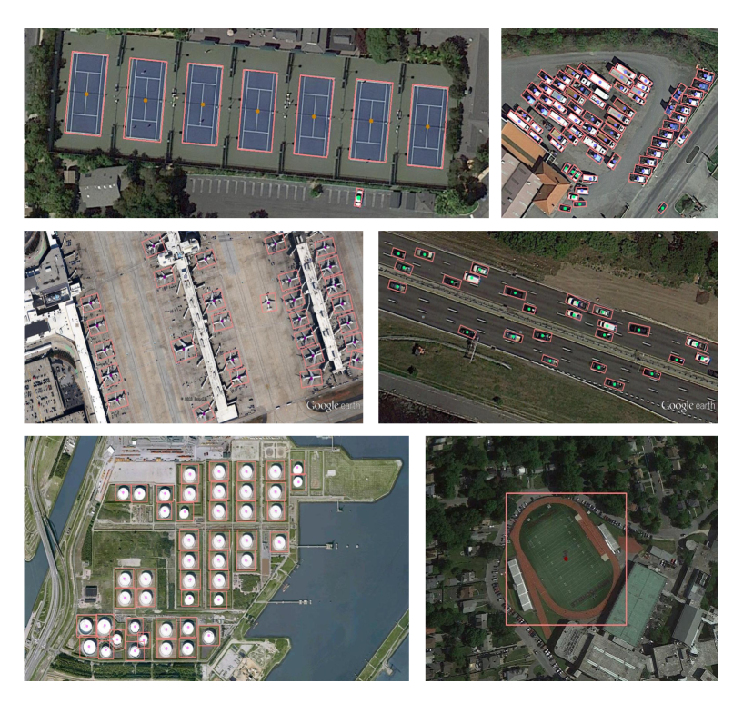
Figure 7: High quality outputs of P-RSDet on DOTA, UCAS-AOD, NWPU VHR-10.

IV-C1 Oriented Bounding Boxes

As shown in Table I and II, our P-RSDet achieve satisfactory $72.30\%$ mAP on DOTA, and $90.03\%$ mAP on UCAS-AOD with the output form of oriented bounding boxes. Compared with the anchor-based detectors modeled in Cartesian coordinate system, our model is more competitive in the task of detecting oriented objects for remote sening images with simpler design and higher accuracy.

IV-C2 Horizontal Bounding Boxes

In order to verify the excellent general capability of our model, we do the experiments on UCAS-AOD and NWPU VHR-10 datasets with the annotations of horizontal bounding box. As shown in Table II and III, P-RSDet gets $90.24\%$ mAP and $90.80\%$ mAP on these two datasets respectively.

Experimental results show that our model has excellent performance in both horizontal and oriented detection tasks. P-RSDet successfully integrates the two types of detectors in the remote sensing field with minimum computational cost via the combination of anchor-free and polar coordinates.

TABLE IV: Comparisons of Different Encoder-Decoders.

Encoder-Decoders	plane	car	mAP
ResNet-101	92.69	87.38	90.03
DLA-34	91.02	85.24	88.13
104-Hourglass	94.15	89.29	91.72

TABLE V: Effects of Polar RingLoss.

Polar Ring Area Loss	plane	car	mAP
With Polar RingLoss	92.69	87.38	90.03
Without Polar RingLoss	91.21	85.16	88.18

TABLE VI: Comparisons of Different Polar Points Extraction Methods.

Extraction Methods	plane	car	mAP
P-RSDet(ours)	92.69	87.38	90.03
Top 100	90.02	81.85	85.93

IV-D Ablation Studies

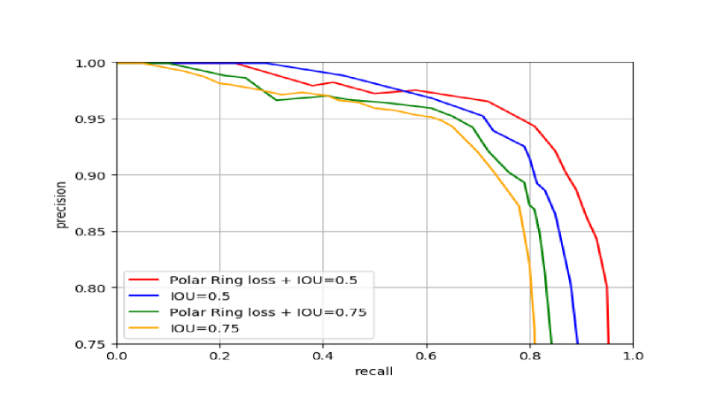
Figure 8: The P-R curves in different situations. Red line: With Polar Ring Loss and IOU=0.5. Blue line: Without Polar Ring Loss and IOU=0.5. Green line: With Polar Ring Loss and IOU=0.75. Orange line: Without Polar Ring Loss and IOU=0.75.

In this section, we show the results of ablation experiments from three aspects: different encoder-decoder, Polar RingLoss and different methods of extracting polar points.

Different Encoder-Decoder: In P-RSDet, we use a high resolution ResNet-101 modified in [21] as the Encoder-Decoder. For the sake of testing the influences of different Encoder-Decoders on our model, we replace the ResNet-101 with DLA-34[21] [47] and 104-Hourglass[19][48]. DLA-34 and 104-Hourglass are two backbone networks smaller and larger than ResNet-101 respectively. We do the experiments on UCAS-AOD with oriented bounding box.

As shown in Table IV, our model can still achieve satisfactory results of $88.1\%$ mAP when using small DLA-34 as the Encoder-Decoder. It is noteworthy that the performance of our model can be further improved when we choose the stronger 104-Hourglass. Experiments show that our model is effective with different Encoder-Decoders.

Polar Ring Area Loss: As mentioned in Section III-D, we design a new Polar-RingLoss for our P-RSDet. In order to verify its effectiveness, we design this comparative experiment on UCAS-AOD with oriented bounding box.

In the experiment with Polar Ring Area Loss, we set its weight to 0.01. As shown in Table V, our model with Polar Ring Area Loss outperforms the one without Polar Ring Area Loss by $1.85\%$ mAP. Fig. 8 shows the Precision-Recall curves in different situations. When Recall remains the same, higher Precision means better performace. It can be seen that whether IOU equals 0.5 or 0.75, precision of the model with Polar Ring Area Loss declines more slowly, so the performance is better. Therefore, the design of Polar Ring Area Loss is effective for P-RSDet.

Different Method of Extracting Polar Points: We optimize the keypoints extraction methods of CornerNet[19] compare the results of our new method with it. In the comparative experienment, we pick top 100 points in the heatmap as the pole points according to the extraction method in [19]. We also do this experiments on UCAS-AOD with the detection of oriented objects. As shown in Table VI, the method which picks top $100$ points as pole points only achieves $85.93\%$ mAP because there are more than $100$ targets in many remote sensing images. In the horizontal bounding box detection of UCAS-AOD and NWPU-VHR-10 as shown in Table II and Table III, we also believe that the performance improvement is partly due to this new extracting method, because the low missed detection rate will greatly improve the detection performance.

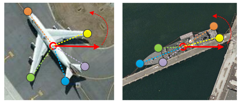
Figure 9: In polar coordinates, P-RSDet can be transplanted to more precise keypoint detection tasks by simply increasing the number of polar radius $\rho$ and polar angles $\theta$ in regression.

V Conclusion and Outlook

A novel object detector named P-RSDet is proposed for remote sensing images via the combination of polar coordinates and anchor-free. By introducing polar coordinates, P-RSDet can detect objects with the annotation forms of both the horizontal and oriented bounding boxes in a simple and efficient way. By adopting the anchor free model, the missed detection caused by NMS in the anchor-based model is avoided, making P-RSDet suitable for detecting densely arranged remote sensing objects. In order to make the output results more accurate, we also optimize a new method of extracting pole points and design a special Polar Ring Area Loss for our model. Experimental results on multiple datasets show that the detector modeling in polar coordinates is effective.

In addition, we believe that our model can be more widely used through simple adjustment. In the field of remote sensing object detection, to get more accurate object information, some datasets are labeled in the form of keypoints such as Aircraft-KP[45] which marks five keypoints of each aircraft. Our P-RSDet can be migrated to a more accurate keypoints dataset by simply increasing the number of regression values in polar coordinates. As shown in Figure 9 , our modeling process on keypoints datasets by regressing five polar radii and five polar angles.

VI Acknowledgment

We thank our colleagues for helpful suggestions and discussions with regard to this work.

References

- [1] P. Wang, X. Sun, W. Diao, and K. Fu, “Mergenet: Feature-merged network for multi-scale object detection in remote sensing images,” in IGARSS 2019-2019 IEEE International Geoscience and Remote Sensing Symposium. IEEE, 2019, pp. 238–241.
- [2] Z. Deng, H. Sun, S. Zhou, J. Zhao, L. Lei, and H. Zou, “Multi-scale object detection in remote sensing imagery with convolutional neural networks,” ISPRS journal of photogrammetry and remote sensing, vol. 145, pp. 3–22, 2018.
- [3] P. Ding, Y. Zhang, W.-J. Deng, P. Jia, and A. Kuijper, “A light and faster regional convolutional neural network for object detection in optical remote sensing images,” ISPRS journal of photogrammetry and remote sensing, vol. 141, pp. 208–218, 2018.
- [4] S. Zhang, L. Wen, X. Bian, Z. Lei, and S. Z. Li, “Single-shot refinement neural network for object detection,” in Proceedings of the IEEE conference on computer vision and pattern recognition, 2018, pp. 4203–4212.
- [5] S. Ren, K. He, R. Girshick, and J. Sun, “Faster r-cnn: Towards real-time object detection with region proposal networks,” in Advances in neural information processing systems, 2015, pp. 91–99.
- [6] K. He, X. Zhang, S. Ren, and J. Sun, “Deep residual learning for image recognition,” in Proceedings of the IEEE conference on computer vision and pattern recognition, 2016, pp. 770–778.
- [7] T.-Y. Lin, P. Dollár, R. Girshick, K. He, B. Hariharan, and S. Belongie, “Feature pyramid networks for object detection,” in Proceedings of the IEEE conference on computer vision and pattern recognition, 2017, pp. 2117–2125.
- [8] J. Redmon and A. Farhadi, “Yolov3: An incremental improvement,” arXiv preprint arXiv:1804.02767, 2018.
- [9] W. Liu, D. Anguelov, D. Erhan, C. Szegedy, S. Reed, C.-Y. Fu, and A. C. Berg, “Ssd: Single shot multibox detector,” in European conference on computer vision. Springer, 2016, pp. 21–37.
- [10] T.-Y. Lin, P. Goyal, R. Girshick, K. He, and P. Dollár, “Focal loss for dense object detection,” in Proceedings of the IEEE international conference on computer vision, 2017, pp. 2980–2988.
- [11] Z. Cai and N. Vasconcelos, “Cascade r-cnn: Delving into high quality object detection,” in Proceedings of the IEEE conference on computer vision and pattern recognition, 2018, pp. 6154–6162.
- [12] J. Ma, W. Shao, H. Ye, L. Wang, H. Wang, Y. Zheng, and X. Xue, “Arbitrary-oriented scene text detection via rotation proposals,” IEEE Transactions on Multimedia, vol. 20, no. 11, pp. 3111–3122, 2018.
- [13] Y. Jiang, X. Zhu, X. Wang, S. Yang, W. Li, H. Wang, P. Fu, and Z. Luo, “R2cnn: rotational region cnn for orientation robust scene text detection,” arXiv preprint arXiv:1706.09579, 2017.
- [14] X. Yang, H. Sun, K. Fu, J. Yang, X. Sun, M. Yan, and Z. Guo, “Automatic ship detection in remote sensing images from google earth of complex scenes based on multiscale rotation dense feature pyramid networks,” Remote Sensing, vol. 10, no. 1, p. 132, 2018.
- [15] X. Yang, J. Yang, J. Yan, Y. Zhang, T. Zhang, Z. Guo, X. Sun, and K. Fu, “Scrdet: Towards more robust detection for small, cluttered and rotated objects,” in Proceedings of the IEEE International Conference on Computer Vision, 2019, pp. 8232–8241.
- [16] H. Wei, L. Zhou, Y. Zhang, H. Li, R. Guo, and H. Wang, “Oriented objects as pairs of middle lines,” arXiv preprint arXiv:1912.10694, 2019.
- [17] Y. Wang, Y. Zhang, Y. Zhang, L. Zhao, X. Sun, and Z. Guo, “Sard: Towards scale-aware rotated object detection in aerial imagery,” IEEE Access, vol. 7, pp. 173 855–173 865, 2019.
- [18] J. Redmon, S. Divvala, R. Girshick, and A. Farhadi, “You only look once: Unified, real-time object detection,” in Proceedings of the IEEE conference on computer vision and pattern recognition, 2016, pp. 779–788.
- [19] H. Law and J. Deng, “Cornernet: Detecting objects as paired keypoints,” in Proceedings of the European Conference on Computer Vision (ECCV), 2018, pp. 734–750.
- [20] X. Zhou, J. Zhuo, and P. Krahenbuhl, “Bottom-up object detection by grouping extreme and center points,” in Proceedings of the IEEE Conference on Computer Vision and Pattern Recognition, 2019, pp. 850–859.
- [21] X. Zhou, D. Wang, and P. Krähenbühl, “Objects as points,” arXiv preprint arXiv:1904.07850, 2019.
- [22] Z. Tian, C. Shen, H. Chen, and T. He, “Fcos: Fully convolutional one-stage object detection,” in Proceedings of the IEEE international conference on computer vision, 2019, pp. 9627–9636.
- [23] K. Fu, W. Lu, W. Diao, M. Yan, H. Sun, Y. Zhang, and X. Sun, “Wsf-net: Weakly supervised feature-fusion network for binary segmentation in remote sensing image,” Remote Sensing, vol. 10, no. 12, p. 1970, 2018.
- [24] J. Dai, Y. Li, K. He, and J. Sun, “R-fcn: Object detection via region-based fully convolutional networks,” in Advances in neural information processing systems, 2016, pp. 379–387.
- [25] T. Kong, A. Yao, Y. Chen, and F. Sun, “Hypernet: Towards accurate region proposal generation and joint object detection,” in Proceedings of the IEEE conference on computer vision and pattern recognition, 2016, pp. 845–853.
- [26] K. He, G. Gkioxari, P. Dollár, and R. Girshick, “Mask r-cnn,” in Proceedings of the IEEE international conference on computer vision, 2017, pp. 2961–2969.
- [27] K. Fu, Z. Chang, Y. Zhang, G. Xu, K. Zhang, and X. Sun, “Rotation-aware and multi-scale convolutional neural network for object detection in remote sensing images,” ISPRS Journal of Photogrammetry and Remote Sensing, vol. 161, pp. 294–308, 2020.
- [28] J. Redmon and A. Farhadi, “Yolo9000: better, faster, stronger,” in Proceedings of the IEEE conference on computer vision and pattern recognition, 2017, pp. 7263–7271.
- [29] P. Lyu, C. Yao, W. Wu, S. Yan, and X. Bai, “Multi-oriented scene text detection via corner localization and region segmentation,” in Proceedings of the IEEE conference on computer vision and pattern recognition, 2018, pp. 7553–7563.
- [30] J. Ding, N. Xue, Y. Long, G.-S. Xia, and Q. Lu, “Learning roi transformer for oriented object detection in aerial images,” in Proceedings of the IEEE Conference on Computer Vision and Pattern Recognition, 2019, pp. 2849–2858.
- [31] S. Gai, F. Da, and X. Fang, “A novel camera calibration method based on polar coordinate,” Plos one, vol. 11, no. 10, p. e0165487, 2016.
- [32] L. Zhang, H. Guo, H. Jiao, G. Liu, G. Shen, and W. Wu, “A polar coordinate system based on a projection surface for moon-based earth observation images,” Advances in Space Research, vol. 64, no. 11, pp. 2209–2220, 2019.
- [33] B. Gergič, P. Planinšič, B. Banjanin, D. Gleich, and Ž. Čučej, “A comparison between sar data compression in cartesian and polar coordinates,” International Journal of Remote Sensing, vol. 25, no. 10, pp. 1987–1994, 2004.
- [34] W. Zhang, X. Sun, K. Fu, C. Wang, and H. Wang, “Object detection in high-resolution remote sensing images using rotation invariant parts based model,” IEEE Geoscience and Remote Sensing Letters, vol. 11, no. 1, pp. 74–78, 2013.
- [35] W. Zhang, X. Sun, H. Wang, and K. Fu, “A generic discriminative part-based model for geospatial object detection in optical remote sensing images,” ISPRS journal of photogrammetry and remote sensing, vol. 99, pp. 30–44, 2015.
- [36] R. Girshick, “Fast r-cnn,” in Proceedings of the IEEE international conference on computer vision, 2015, pp. 1440–1448.
- [37] G.-S. Xia, X. Bai, J. Ding, Z. Zhu, S. Belongie, J. Luo, M. Datcu, M. Pelillo, and L. Zhang, “Dota: A large-scale dataset for object detection in aerial images,” in Proceedings of the IEEE Conference on Computer Vision and Pattern Recognition, 2018, pp. 3974–3983.
- [38] H. Zhu, X. Chen, W. Dai, K. Fu, Q. Ye, and J. Jiao, “Orientation robust object detection in aerial images using deep convolutional neural network,” in 2015 IEEE International Conference on Image Processing (ICIP). IEEE, 2015, pp. 3735–3739.
- [39] G. Cheng, P. Zhou, and J. Han, “Learning rotation-invariant convolutional neural networks for object detection in vhr optical remote sensing images,” IEEE Transactions on Geoscience and Remote Sensing, vol. 54, no. 12, pp. 7405–7415, 2016.
- [40] A. Paszke, S. Gross, S. Chintala, G. Chanan, E. Yang, Z. DeVito, Z. Lin, A. Desmaison, L. Antiga, and A. Lerer, “Automatic differentiation in pytorch,” 2017.
- [41] D. P. Kingma and J. Ba, “Adam: A method for stochastic optimization,” arXiv preprint arXiv:1412.6980, 2014.
- [42] M. Everingham, L. Van Gool, C. K. Williams, J. Winn, and A. Zisserman, “The pascal visual object classes (voc) challenge,” International journal of computer vision, vol. 88, no. 2, pp. 303–338, 2010.
- [43] S. M. Azimi, E. Vig, R. Bahmanyar, M. Körner, and P. Reinartz, “Towards multi-class object detection in unconstrained remote sensing imagery,” in Asian Conference on Computer Vision. Springer, 2018, pp. 150–165.
- [44] J. Ding, N. Xue, Y. Long, G.-S. Xia, and Q. Lu, “Learning roi transformer for detecting oriented objects in aerial images,” arXiv preprint arXiv:1812.00155, 2018.
- [45] H. Wei, Y. Zhang, B. Wang, Y. Yang, H. Li, and H. Wang, “X-linenet: Detecting aircraft in remote sensing images by a pair of intersecting line segments,” IEEE Transactions on Geoscience and Remote Sensing, 2020.
- [46] C.-Y. Fu, W. Liu, A. Ranga, A. Tyagi, and A. C. Berg, “Dssd: Deconvolutional single shot detector,” arXiv preprint arXiv:1701.06659, 2017.
- [47] J. Dai, H. Qi, Y. Xiong, Y. Li, G. Zhang, H. Hu, and Y. Wei, “Deformable convolutional networks,” in Proceedings of the IEEE international conference on computer vision, 2017, pp. 764–773.
- [48] A. Newell, K. Yang, and J. Deng, “Stacked hourglass networks for human pose estimation,” in European conference on computer vision. Springer, 2016, pp. 483–499.