Examining the secondary product origin of cosmic ray positrons with the latest AMS-02 data

Abstract

Measurements of cosmic-ray (CR) positron fraction by PAMELA and other experiments have found an excess above 10 GeV relative to the standard predictions for secondary production in the interstellar medium (ISM). Although the excess has been mostly suggested to arise from some primary sources of positrons (such as pulsars and or annihilating dark matter particles), the almost constant flux ratio of $e^{+}/\bar{p}$ argues for an alternative possibility that the excess positrons and antiprotons up to the highest energies are secondary products generated in hadronic interactions. Recently, Yang & Aharonian (2019) revisit this possibility by assuming the presence of an additional population of CR nuclei sources. Here we examine this secondary product scenario using the DRAGON code, where the radiative loss of positrons is taken into account consistently. We confirm that the CR proton spectrum and the antiproton data can be explained by assuming the presence of an additional population of CR sources. However, the corresponding positron spectrum deviates from the measured data significantly above 100 GeV due to the strong radiative cooling. This suggests that, although hadronic interactions can explain the antiproton data, the corresponding secondary positron flux is still not enough to account for the AMS data. Hence contribution from some primary positron sources, such as pulsars or dark matter, is non-negligible.

3

1. introduction

Inelastic interactions of primary cosmic rays (CRs) with the interstellar medium are expected to produce secondary positrons and anti-protons with quite soft spectra. Unexpected spectra excess of positrons and antiprotons relative to the standard prediction has been detected at energies exceeding $E\gtrsim 10\,$GeV by PAMELA(Adriani et al., 2009; Ackermann et al., 2012), the Alpha Magnetic Spectrometer(AMS-02)(Kounine, 2015; Aguilar et al., 2019) and other experiments. The most popular model for the positron excess is that it arises from some primary sources of positrons such as pulsars (e.g., (Hooper et al., 2009; Yin et al., 2013; Profumo, 2012; Joshi, & Razzaque, 2017)), or annihilating dark matter particles (e.g., (Cholis, & Hooper, 2013; Yin et al., 2009)). However, measurements on the positron and antiproton flux by AMS-02 have revealed that the flux ratio $e^{+}/\bar{p}$ keeps an almost constant value of $\simeq 2$ in the energy range of 30-300 GeV, coincident with the expected ratio of $e^{+}/\bar{p}$ produced as secondary particles from hadronic interactions of cosmic ray (CR) protons (Lipari, 2017, 2019). Motivated by this coincidence, it is suggested that the excesses of positrons and antiprotons may result also from hadronic interactions (Lipari, 2017, 2019; Katz et al., 2010; Blum et al., 2013). To explain the positron excess, Lipari (2017, 2019) assume an energy independent diffusion coefficient and negligible energy losses up to the maximum energy observed (around TeV). Recently, Yang & Aharonian (2019) suggest that an additional population of primary CR nuclei sources beside the normal population of sources might have produced the excess secondary particles through the CR hadronic interactions.

However, positrons would suffer from efficient radiative loss in magnetic field and interstellar radiation field (ISRF) during their propagation in the interstellar medium (ISM), while anti-protons do not. Thus, the $e^{+}/\bar{p}$ ratio in the propagated CR spectrum may not remain $\simeq 2$ at high energy as it does in the spectrum at generation. Recently, AMS-02 has released the latest measurement of CR positron data. The new measurement not only increases the statistics by a factor of three, but also extends the spectrum up to an unprecedentedly high energy, $\lesssim 1\,$TeV, and reveals a marked dropoff at the high-energy end (Aguilar et al., 2019). In the secondary origin model, one would naively expect a dropoff due to stronger radiative cooling for higher energy positrons. However, the exact position of the steepening due to radiative cooling depends on specific physical conditions, such as the magnetic fields in the galactic halo and the residence time of positrons. The precise measurement of AMS-02 on the positron spectrum motivates us to conduct a critical study of whether the new positron data can be explained simultaneously with the antiproton data in the framework of the secondary origin model assuming the presence of an additional population of primary CR sources.

Two classes of the additional population sources of the primary CRs (i.e., the cosmic-ray accelerators) have been suggested. One is that a single nearby supernova remnant (SNR) accelerates cosmic ray protons, which interact with a presumed dense gas cloud and produce secondary positrons and antiprotons (e.g., Fujita et al. (2009); Liu et al. (2017)). This model has limitations on the age and the distance of the source, i.e., the age of the SN should be around $10^{5}$ yr and the distance should be $\sim 100$ pc. However, evidence from deposition of ⁶⁰Fe in the deep ocean crust suggests a SN occurred 2 Myr ago(Benítez et al., 2002; Ellis et al., 1996; Fry et al., 2015; Knie et al., 1999), much older than the age required. The other one assumes a continuously distributed source population to produce secondary positrons and antiprotons (Yang & Aharonian, 2019). With less constraints on the sources compared to the former model, the idea proposed by Yang & Aharonian (2019) seems to be more attractive and reasonable. Hence, we do not consider the single SNR scenario, but look into the latter scenario in which more free parameters are introduced for the second CR source population, providing a favourable condition for the reproduction of the excesses in the positron and antiproton spectra. The open code DRAGON (Di Bernardo et al., 2010, 2013; Evoli et al., 2017) is introduced to solve the propagations of CRs and the production of secondary particles.

The paper is organized as follows. In §2, we first attempt to explain the CR proton data measured by DAMPE and other experiments using the DRAGON code. In §3, we calculate the secondary particle flux using DRAGON and compared the results with the corresponding data. We present discussions in §4.

2. model

2.1. Fitting the proton spectrum

CRs spread in the galaxy through diffusive propagation after being injected from sources. In this work, we use DRAGON code to numerically solve the diffusive transport equation. The detailed description of DRAGON can be found in Evoli et al. (2008) and the DRAGON website. With this code, CR nuclei and lepton propagation in the Galaxy can be successfully calculated. In our calculations, the halo is treated as a cylinder, with its radius $R_{\rm{max}}\,=\,12$ kpc. Its half thickness, $L$, is adopted as 4 kpc. The diffusion coefficient $D$ is considered to be spatial independent and described as

$$D(\rho)=D_{0}\beta(\frac{\rho}{\rho_{0}})^{\delta},$$ (1)

where $\beta$ is the CR speed in the unit of speed of light and $\rho$ is the rigidity.

Positrons and antiprotons are produced as secondaries by the hadronic interactions of the primary CRs (mainly protons). We start from the phenomenological fitting to the primary CR proton spectrum below 100 TeV that is relevant for our study. Based on the data of AMS-02 (Aguilar et al., 2014) and DAMPE (An et al., 2019), we divide the proton spectrum into two components. The first one is the conventional background cosmic-ray component (dubbed as the component 1), with the form of a single power law. The initial injection spectrum can be described as

$$N_{1}(\rho)\propto(\frac{\rho}{\rho_{0}})^{-\alpha_{0}}.$$ (2)

Recent observations reveal that the proton spectrum hardens at around 200 GeV (Yoon et al., 2011; An et al., 2019) and softens at $E$ $\simeq$ $10^{4}$ GeV(An et al., 2019). The hardening of the proton spectrum requires a second, hard component, which could originate from some extra sources (dubbed as the component 2), such as young massive stars (Bykov et al., 2013; Aharonian et al., 2019). We find that the initial injection spectrum of this second component can be written by a broken power law,

$$N_{2}(E)\propto\left\{\begin{array}[]{ll}(\frac{\rho}{\rho_{1}})^{-\alpha_{1}},&{\rm if}\,\,\rho<\rho_{1},\\ (\frac{\rho}{\rho_{1}})^{-\alpha_{2}},&{\rm if}\,\,\rho\geqslant\rho_{1},\end{array}\right.$$ (3)

The respective contributions to proton flux from these two populations and the sum of them are shown in Fig. 1, confronting with the measurement of AMS-02, DAMPE and ARGO experiments (Aguilar et al., 2014; An et al., 2019; Amenomori et al., 2011). The adopted parameters are listed in Table 1.

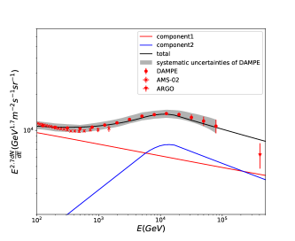
Figure 1.— Fit of the proton spectrum with two source populations of CRs . The red and blue lines represent the contributions from component 1 and component 2, respectively. The total flux is shown by the black line.

2.2. Calculation for the secondary particle flux

During the propagation in the galaxy, primary CRs injected by two populations would interact with ISM and produce secondary particles. With DRAGON code, we can obtain these secondary CR fluxes when calculating the proton spectra simultaneously. Since these secondary particles are produced through hadronic interactions with ISM, we dub them as ISM-component 1 and ISM-component 2, respectively.

In Yang & Aharonian (2019), the leaky box model is used to calculate the secondary particle flux. They find that the secondary particles from the interaction between primary CRs and ISM (ISM-component 1 and ISM-component 2) are not enough to explain the antiproton data. To solve this problem, an extra grammage $X_{s}$ inside the second sources is introduced to produce additional antiparticles.

During the propagation of CRs, the magnetic field would scatter these particles in random motion with characteristic velocities relative to the Alfvèn speed ($v_{A}$), which causes a diffusion in momentum and results in a second-order Fermi acceleration. This process is referred as ”reacceleration” (Heinbach & Simon, 1995) (see also Blasi (2004) for reacceleration via the first-order Fermi acceleration). Reacceleration can be taken into account in the DRAGON code. We find that the extra grammage is not necessary when the reacceleration is taken into account. This is because that when considering reacceleration, a smaller $\delta$ can be adopted to fit the B/C ratio. With a smaller $\delta$, the secondary particle spectrum becomes harder, and leads to more anti-protons above $\sim 100$ GeV produced by primary protons during the propagation in the ISM.

On the premise of fitting both the proton flux and the antiproton flux, the simultaneously obtained positron flux, however, significantly deviates from the AMS-02 data, as will be discussed in the next section.

3. results

The resultant B/C ratio, antiproton flux and positron flux are shown in Fig. 2, as a function of energy per nucleon $E\,=\,\frac{Ze\rho}{A}$, where $e$ is the charge of a proton, $Z$ and $A$ are the atomic and mass number. For protons, antiprotons and positrons, $E\,=\,e\rho$. For other nuclei, $E\,\approx\,0.5e\rho$.

The models and parameters we used are listed in Table 1. The spatial distributions for the two source components are considered to be the same.

Table 1Model parameter values for the propagation and the magnetic field used in the DRAGON code. In our calculation, we use the spatial distribution of two source populations provided by Ferrière (2001), the gas distribution provided by Strong et al. (2004), and the geometry of the galaxy magnetic field provided by Pshirkov et al. (2011). $A_{1}$ and $A_{2}$ are the normalization fluxes of ISM-component 1 and ISM-component 2 at 100 $\rm{GeV}$, respectively (in unit of $\rm{GeV}^{-1}\cdot\rm{m}^{-2}\cdot\rm{s}^{-1}\cdot\rm{sr}^{-1}$).

Model/Parameter	Option/Value
Grid Type	2D
$R_{\rm{max}}$	12 kpc
$L$	4 kpc
Gas Distribution	Galprop
Source Distribution	Ferriere
Diffusion type	Constant
$D_{0}$	$4.3\times 10^{28}$ $\rm{cm^{2}/s}$
$\rho_{0}$	4 GV
$\delta$	0.4
$v_{A}$	30 km/s
Magnetic Field Type	Pshirkov
$B_{0}^{\rm{disk}}$	$2.0\times 10^{-6}$ Gauss
$B_{0}^{\rm{halo}}$	$4.0\times 10^{-6}$ Gauss
$B_{0}^{\rm{turb}}$	$7.5\times 10^{-6}$ Gauss
$A_{1}$	$3.8\times 10^{-2}$
$A_{2}$	$4.9\times 10^{-3}$
$\alpha_{0}$	2.4
$\alpha_{1}$	1.9
$\alpha_{2}$	2.5
$\rho_{1}$	12000 GV

The B/C ratios of two source components are shown in Fig. 2(a), where the ratios from two components are the same. In Fig. 2(b), contributions to antiprotons from the ISM-component 1 and the ISM-component 2 are shown by the red and blue lines, respectively. Our results show that the antiproton data can be well explained by the sum of two components. Contributions to positrons by two source components are shown in Fig. 2(c). For high-energy positrons, the radiative cooling due to the synchrotron radiation and inverse Compton scattering is important. As shown by the black solid line, the fluxes drop dramatically starting from $\sim$ 10 GeV. To illustrate the importance of cooling effect on positrons, we also show the case without considering the cooling, denoted by the black dashed line in Fig. 2(c). Without considering any energy losses, the $e^{+}/\bar{p}$ ratio is around 2, consistent with theoretical expectation (Lipari, 2017, 2019). Since there are uncertainties in the strength of the magnetic field and the interstellar radiation field (ISRF), we also consider an extreme case for illustration, where only the cooling due to CMB photons are taken into account (see the black dashed-dotted line). In such a case, the positron flux still cannot explain the AMS-02 data.

The above results can be understood by comparing the residence timescale of CRs, $\tau_{\rm res}$, with the radiative cooling timescale of positrons, $\tau_{\rm c}$. The former one can be derived from the so-called ”grammage”, which measures the amount of material that CRs collide with before they leave the Galaxy. The grammage is defined by $X(E)={\bar{n}}m_{p}\tau_{\rm res}(E)c$, where ${\bar{n}}$ is the average density of gas in the Galaxy, $m_{p}$ is the mass of a proton, and $c$ is the speed of light. The ratio between the secondary CR flux and their parent primary CR flux, such as the B/C ratio, is only sensitive to the grammage accumulated during the propagation. In the leaky-box approximation, this ratio can be written as (Katz et al., 2010; Yang & Aharonian, 2019)

$$R(E)=\frac{\frac{X(E)}{m_{p}}\sigma_{p\rightarrow s}}{1+\sigma_{t}\frac{X(E)}{m_{p}}}.$$ (4)

Here $\sigma_{p\rightarrow s}$ is the differential cross section for the production of secondary particle, and $\sigma_{t}$ is the total inelastic cross section of a certain species of secondary particle. By fitting the B/C data, we obtain $X(E)\,=\,2.1(\frac{E}{300\,\rm{GeV}})^{-0.4}\,\rm{g/cm^{2}}$.

Then we can estimate the residence timescale given an average gas density of ${\bar{n}}=n_{\rm ISM}(l/L)$ (Gabici et al., 2019), where $n_{\rm ISM}\,\sim\,1\,\rm{cm^{-3}}$ is the average density in the Galactic disk, $l\,\sim\,150$ pc is the height of the disk, and $L$ is the height of the CR halo. Adopting a typical height of $L\,=\,4$ kpc and the grammage obtained above, we find the residence time of CRs is $\tau_{\rm{res}}\simeq 26\,{\rm Myr}$ at 300 GeV.

The main uncertainty in the above estimate lies in the height, $L$, of the CR halo. According to previous studies, the typical height of CR halo is $3-10$ kpc (e.g., Orlando & Strong, 2013; Evoli et al., 2020; Moskalenko et al., 2001; Trotta et al., 2011). Combining $\tau_{\rm{res}}(E)\,=\,L^{2}/D(E)$ with $X(E)=n_{\rm ISM}(l/L)m_{p}\tau_{res}(E)c$, we get $\tau_{\rm res}(E)\,=\,26\,(\frac{L}{4\,\rm{kpc}})(\frac{E}{300\,{\rm{GeV}}})^{-0.4}\,\rm{Myr}$ when the grammage is fixed.

On the other hand, the cooling timescale of positrons, $\tau_{\rm c}$, can be given by

$$\tau_{\rm c}(E)\,=\,2.5\,\,(\frac{300\,\rm GeV}{E})\,(\frac{1\,{\rm{eV/cm^{3}}}}{U_{B}\,+\,U_{ph}})\,\rm{Myr},$$ (5)

where $E$ is the energy of positrons, $U_{B}$ is the energy density of the magnetic field and $U_{ph}$ is the energy density of the radiation field. In the extreme assumption that only IC cooling due to the CMB radiation is considered, i.e., $U_{B}\,+\,U_{ph}\,=\,U_{\rm{CMB}}\,=\,0.26\,{\rm{eV/cm^{3}}}$, we obtain $\tau_{\rm c}(300\,\rm{GeV})\,=\,10$ Myr, which is already shorter than $\tau_{\rm{res}}(300\,\rm{GeV})\,\gtrsim\,20\,\rm{Myr}$. Therefore, any secondary-origin scenarios can not explain the positron data because of the severe radiative cooling.

Recent measurements by AMS-02 shows that the spectral indices of secondary-to-primary ratio (e.g., Li/C, Be/C, B/C) exhibit a hardening of $0.13\,\pm\,0.03$ above 200 GV (Aguilar et al., 2018). This may indicate that the slope ($\delta$) of the diffusion coefficient becomes smaller above 200 GV. As a smaller $\delta$ at high energy implies that the diffusion coefficient increases with energy more slowly, we obtain a larger residence timescale ($\tau_{\rm res}\propto 1/D$), given that the residence timescale below 200 GV is fixed. That is, $\tau_{\rm res}(E)\,=\,30\,(\frac{L}{4\,\rm{kpc}})(\frac{E}{300\,{\rm{GeV}}})^{-0.27}\,\rm{Myr}$ for $E\,\geqslant\,100\,\rm{GeV}$, if $\tau_{\rm{res}}(E\,\leqslant\,100\,\rm{GeV})$ is normalized to fit the B/C data. Thus, the cooling effect of positrons will be more significant in this case.

Note that the scarcity of the positron flux above several tens of GeV cannot be compensated by introducing an additional positron component of secondary origin, since otherwise the co-produced antiproton flux will overshoot the data. As a result, we conclude the secondary positron flux from the hadronic interactions is insufficient to account for the AMS-02 positron data when the spectrum of accompanying antiprotons is tuned to match the data.

4. Discussions and Conclusions

In summary, by using the DRAGON code, we have shown that the CR proton data can be explained by two population of sources and the hadronic interaction of these CR protons with ISM can explain the antiproton data. However, the secondary positron flux simultaneously produced in this hadronic interaction model is insufficient to explain the measured data. This is due to the severe radiative energy losses of high-energy positrons, which demonstrates that some primary sources of positrons, such as dark matters and pulsars (e.g., Aharonian et al., 1995; Atoyan et al., 1995; Hooper et al., 2009; Fang et al., 2019), are needed at higher energies to account for the additional positron fluxes.

We find that the extra grammage introduced by Yang & Aharonian (2019) is not needed when the diffusive reacceleration is considered in the code. There has been suggestion that diffusive reacceleration is helpful in explaining the B/C ratio at low energy, given that 50% of the total CR power is provided by reacceleration (Drury, & Strong, 2017). However, whether the reacceleration really occurs at the required level is unknown (e.g., Gabici et al. (2019)), and further studies are needed to determine the contributions of reacceleration to the total CR power. On the other hand, whether the reacceleration presents or not does not change our conclusion about the secondary positron flux. As long as the antiproton flux matches data, the positron flux is insufficient to account for the AMS-02 data due to the radiative cooling.

Some alternative secondary production scenarios, like the Nested Leaky Box (NLB) model (e.g., Cowsik et al., 2014) do not need to introduce the CR halo. Instead, the model assumes an energy-independent diffusion coefficient or CR residence timescale above $\sim 200\,$GeV. As a result, TeV CRs can still have sufficient time to get isotropized before leaving Galaxy, and positrons of $\sim 100\,$GeV can quickly leave Galaxy before cooling. However, the key assumption of the model, i.e., an energy-independent residence timescale above 200 GeV, is inconsistent with the latest AMS-02 observation on the B/C ratio, as explicitly pointed out by Aguilar et al. (2016).

The secondary positrons could also be accelerated in a subset of supernova remnant shocks which propagate into molecular clouds that are positively charged by cosmic-ray protons (Dogiel & Sharov, 1990; Malkov et al., 2016). The acceleration could harden the positron spectrum. However, the maximum energy that this mechanism can work is limited to be less than 100 GeV according to the current understanding (Dogiel & Sharov, 1990; Malkov et al., 2016).

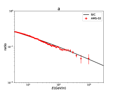
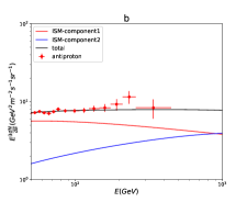
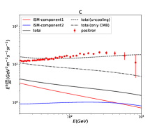
Figure 2.— Modelings of the B/C ratio (left panel), antiproton flux (middle panel) and positron flux (right panel). The data of B/C ratio are taken from Aguilar et al. (2016). The data of antiproton and positron fluxes are taken from Aguilar et al. (2016) and Aguilar et al. (2019), respectivly. The red and the blue lines represent the antiparticles produced from the ISM-component 1 and 2, respectively. The black solid line is the total flux. In the right panel, the black dashed line represents the total positron flux without considering the radiative cooling, and the black dashed-dotted line represents the total positron flux when only the inverse-Compton cooling due to CMB photons is considered.

References

- Ackermann et al. (2012) Ackermann, M., Ajello, M., Allafort, A., et al. 2012, Phys. Rev. Lett., 108, 011103
- Adriani et al. (2009) Adriani, O., Barbarino, G. C., Bazilevskaya, G. A., et al. 2009, Nature, 458, 607
- Aguilar et al. (2014) Aguilar, M., Aisa, D., Alvino, A., et al. 2014, Physical Review Letters, 113, 121102
- Aguilar et al. (2016) Aguilar, M., Ali Cavasonza, L., Alpat, B., et al. 2016, Physical Review Letters, 117, 091103
- Aguilar et al. (2016) Aguilar, M., Ali Cavasonza, L., Ambrosi, G., et al. 2016, Physical Review Letters, 117, 231102
- Aguilar et al. (2018) Aguilar, M., Ali Cavasonza, L., Ambrosi, G., et al. 2018, Phys. Rev. Lett., 120, 021101
- Aguilar et al. (2019) Aguilar, M., Ali Cavasonza, L., Ambrosi, G., et al. 2019, Physical Review Letters, 122, 041102
- Aharonian et al. (1995) Aharonian, F. A., Atoyan, A. M., & Voelk, H. J. 1995, A&A, 294, L41
- Aharonian et al. (2019) Aharonian, F., Yang, R., & de Oña Wilhelmi, E. 2019, Nature Astronomy, 3, 561
- Amenomori et al. (2011) Amenomori, M., Bi, X. J., Chen, D., et al. 2011, Astrophysics and Space Sciences Transactions, 7, 15
- An et al. (2019) An, Q., Asfandiyarov, R., Azzarello, P., et al. 2019, arXiv e-prints, arXiv:1909.12860
- Atoyan et al. (1995) Atoyan, A. M., Aharonian, F. A., & Völk, H. J. 1995, Phys. Rev. D, 52, 3265
- Benítez et al. (2002) Benítez, N., Maíz-Apellániz, J., & Canelles, M. 2002, Physical Review Letters, 88, 081101
- Blasi (2004) Blasi, P. 2004, Astroparticle Physics, 21, 45
- Blum et al. (2013) Blum, K., Katz, B., & Waxman, E. 2013, Phys. Rev. Lett., 111, 211101
- Bykov et al. (2013) Bykov, A. M., Gladilin, P. E., & Osipov, S. M. 2013, MNRAS, 429, 2755
- Cholis, & Hooper (2013) Cholis, I., & Hooper, D. 2013, Phys. Rev. D, 88, 023013
- Cowsik et al. (2014) Cowsik, R., Burch, B., & Madziwa-Nussinov, T. 2014, ApJ, 786, 124
- Di Bernardo et al. (2010) Di Bernardo, G., Evoli, C., Gaggero, D., et al. 2010, Astroparticle Physics, 34, 274
- Di Bernardo et al. (2013) Di Bernardo, G., Evoli, C., Gaggero, D., et al. 2013, JCAP, 2013, 036
- Dogiel & Sharov (1990) Dogiel, A. V., & Sharov, S. G. 1990, International Cosmic Ray Conference, 109
- Drury, & Strong (2017) Drury, L. O. ’C ., & Strong, A. W. 2017, A&A, 597, A117
- Ellis et al. (1996) Ellis, J., Fields, B. D., & Schramm, D. N. 1996, ApJ, 470, 1227
- Erlykin & Wolfendale (2015) Erlykin, A. D., & Wolfendale, A. W. 2015, Astroparticle Physics, 60, 86
- Evoli et al. (2008) Evoli, C., Gaggero, D., Grasso, D., et al. 2008, JCAP, 2008, 018
- Evoli et al. (2017) Evoli, C., Gaggero, D., Vittino, A., et al. 2017, JCAP, 2017, 015
- Evoli et al. (2020) Evoli, C., Morlino, G., Blasi, P., et al. 2020, Phys. Rev. D, 101, 023013
- Fang et al. (2019) Fang, K., Bi, X.-J., & Yin, P.-F. 2019, arXiv e-prints, arXiv:1906.08542
- Ferrière (2001) Ferrière, K. M. 2001, Reviews of Modern Physics, 73, 1031
- Fry et al. (2015) Fry, B. J., Fields, B. D., & Ellis, J. R. 2015, ApJ, 800, 71
- Fujita et al. (2009) Fujita, Y., Kohri, K., Yamazaki, R., & Ioka, K. 2009, Phys. Rev. D, 80, 063003
- Gabici et al. (2019) Gabici, S., Evoli, C., Gaggero, D., et al. 2019, arXiv e-prints, arXiv:1903.11584
- Heinbach & Simon (1995) Heinbach, U., & Simon, M. 1995, ApJ, 441, 209
- Hooper et al. (2009) Hooper, D., Blasi, P., & Serpico, P. D. 2009, JCAP, 2009, 025
- Hooper et al. (2017) Hooper, D., Cholis, I., Linden, T., & Fang, K. 2017, Phys. Rev. D, 96, 103013
- Joshi, & Razzaque (2017) Joshi, J. C., & Razzaque, S. 2017, JCAP, 2017, 029
- Katz et al. (2010) Katz, B., Blum, K., Morag, J., & Waxman, E. 2010, MNRAS, 405, 1458
- Knie et al. (1999) Knie, K., Korschinek, G., Faestermann, T., et al. 1999, Physical Review Letters, 83, 18
- Kounine (2015) Kounine, A. 2015, 34th International Cosmic Ray Conference (ICRC2015), 34, 300
- Lipari (2017) Lipari, P. 2017, Phys. Rev. D, 95, 063009
- Lipari (2019) Lipari, P. 2019, arXiv:1902.06173
- Liu et al. (2017) Liu, W., Bi, X.-J., Lin, S.-J., Wang, B.-B., & Yin, P.-F. 2017, Phys. Rev. D, 96, 023006
- Malkov et al. (2016) Malkov, M. A., Diamond, P. H., & Sagdeev, R. Z. 2016, Phys. Rev. D, 94, 063006
- Moskalenko et al. (2001) Moskalenko, I. V., Mashnik, S. G., & Strong, A. W. 2001, International Cosmic Ray Conference, 1836
- Orlando & Strong (2013) Orlando, E., & Strong, A. 2013, MNRAS, 436, 2127
- Profumo (2012) Profumo, S. 2012, Central European Journal of Physics, 10, 1
- Pshirkov et al. (2011) Pshirkov, M. S., Tinyakov, P. G., Kronberg, P. P., et al. 2011, ApJ, 738, 192
- Strong et al. (2004) Strong, A. W., Moskalenko, I. V., Reimer, O., et al. 2004, A&A, 422, L47
- Su et al. (2010) Su, M., Slatyer, T. R., & Finkbeiner, D. P. 2010, ApJ, 724, 1044
- Tibaldo et al. (2015) Tibaldo, L., Digel, S. W., Casandjian, J. M., et al. 2015, ApJ, 807, 161
- Trotta et al. (2011) Trotta, R., Jóhannesson, G., Moskalenko, I. V., et al. 2011, ApJ, 729, 106
- Yang & Aharonian (2019) Yang, R., & Aharonian, F. 2019, Phys. Rev. D, 100, 063020
- Yin et al. (2009) Yin, P.-F., Yuan, Q., Liu, J., et al. 2009, Phys. Rev. D, 79, 023512
- Yin et al. (2013) Yin, P.-F., Yu, Z.-H., Yuan, Q., et al. 2013, Phys. Rev. D, 88, 023001
- Yoon et al. (2011) Yoon, Y. S., Ahn, H. S., Allison, P. S., et al. 2011, ApJ, 728, 122