Expected Improvement versus Predicted Value in Surrogate-Based Optimization

Abstract.

Surrogate-based optimization relies on so-called infill criteria (acquisition functions) to decide which point to evaluate next. When Kriging is used as the surrogate model of choice (also called Bayesian optimization), one of the most frequently chosen criteria is expected improvement. We argue that the popularity of expected improvement largely relies on its theoretical properties rather than empirically validated performance. Few results from the literature show evidence, that under certain conditions, expected improvement may perform worse than something as simple as the predicted value of the surrogate model. We benchmark both infill criteria in an extensive empirical study on the ‘BBOB’ function set. This investigation includes a detailed study of the impact of problem dimensionality on algorithm performance. The results support the hypothesis that exploration loses importance with increasing problem dimensionality. A statistical analysis reveals that the purely exploitative search with the predicted value criterion performs better on most problems of five or higher dimensions. Possible reasons for these results are discussed. In addition, we give an in-depth guide for choosing the infill criteria based on prior knowledge about the problem at hand, its dimensionality, and the available budget.

1. Introduction

Many real-world optimization problems require significant resources for each evaluation of a given candidate solution. For example, evaluations might require material costs for laboratory experiments or computation time for extensive simulations. In such scenarios, the available budget of objective function evaluations is often severely limited to a few tens or hundreds of evaluations.

One standard method to efficiently cope with such limited evaluation budgets is . Surrogate models of the objective function are based on data-driven models, which are trained using only a relatively small set of observations. Predictions from these models partially replace expensive objective function evaluations. Since the surrogate model is much cheaper to evaluate than the original objective function, an extensive search becomes feasible. In each iteration, one new candidate solution is proposed by the search on the surrogate. The candidate is evaluated on the expensive function and the surrogate is updated with the new data. This process is iterated until the budget of expensive evaluations is depleted.

A frequently used surrogate model is Kriging (also called Gaussian process regression). In Kriging, a distance-based correlation structure is determined with the observed data (Forr08a). The search for the next candidate solution on the Kriging model is guided by a so-called infill criterion or acquisition function.

A straightforward and simple infill criterion is the . The of a Kriging model is an estimation or approximation of the objective function at a given point in the search space (Forr08a). If the surrogate exactly reproduces the expensive objective function, then optimizing the yields the global optimum of the expensive objective function. In practice, especially in the early iterations of the procedure, the prediction of the surrogate will be inaccurate. Many infill criteria do not only consider the raw predicted function value but also try to improve the model quality with each new iteration. This is achieved by suggesting new solutions in promising but unknown regions of the search space. In essence, such criteria attempt to simultaneously improve the local approximation quality of the optimum as well as the global prediction quality of the surrogate.

The criterion is considered as a standard method for this purpose (Jone98a). makes use of the internal uncertainty estimate provided by Kriging. The of a candidate solution increases if the predicted value or the estimated uncertainty of the model rises.

The optimization algorithm might converge to local optima, if solely the is used as an infill criterion. In the most extreme case, if the suggests a solution that is equal to an already known solution, the algorithm might not make any progress at all, instead repeatedly suggesting the exact same solution (Forr08a). Conversely, can yield a guarantee for global convergence, and convergence rates can be analyzed analytically (Bull11a; Wess17a). As a result, is frequently used as an infill criterion.

We briefly examined 24 software frameworks for . We found 15 that use as a default infill criterion, three that use , five that use criteria based on lower or upper confidence bounds (Auer02a), and a single one that uses a portfolio strategy (which includes confidence bounds and , but not ). An overview of the surveyed frameworks is included in the supplementary material. Seemingly, is firmly established.

Despite this, some criticism can be found in the literature. Wessing and Preuss point out that the convergence proofs are of theoretical interest but have no relevance in practice (Wess17a). The most notable issue in this context is the limited evaluation budget that is often imposed on algorithms. Under these limited budgets, the asymptotic behavior of the algorithm can become meaningless. Wessing and Preuss show results where a model-free CMA-ES often outperforms -based EGO within a few hundred function evaluations (Wess17a).

A closely related issue is that many infill criteria, including , define a static trade-off between exploration and exploitation (Gins10a; Lam16a; Wang18a; Wang19a). This may not be optimal. Intuitively, explorative behavior may be of more interest in the beginning, rather than close to the end of an optimization run.

At the same time, benchmarks that compare and are far and few between. While some benchmarks investigate the performance of -based algorithms, they rarely compare to a variant based on (e.g., (Osbo10a; Snoe12a; Hern14a; Nguy16b)). Other authors suggest portfolio strategies that combine multiple criteria. Often, tests of these strategies do not include the in the portfolio (e.g., (Hoff11a; Vasc19a)).

We would like to discuss two exceptions. Firstly, Noe and Husmeier (Noe18a) do not only suggest a new infill criterion and compare it to , but they also compare it to a broad set of other criteria, importantly including . In several of their experiments, seems to perform better than , depending on the test function and the number of evaluations spent. Secondly, a more recent work by De Ath et al. (DeAt19a) reports similar observations. They observe that“Interestingly, Exploit, which always samples from the best mean surrogate prediction is competitive for most of the high dimensional problems” (DeAt19a). Conversely, they observe better performances of explorative approaches on a few, low-dimensional problems.

In both studies, the experiments cover a restricted set of problems where the dimensionality of each specific test function is usually fixed. The influence of test scenarios, especially in terms of the search space dimension, remains to be clarified. It would be of interest, to see how increasing or decreasing the dimension affects results for each problem.

Hence, we raise two tightly connected research questions:

• Can distinct scenarios be identified where outperforms or vice versa?

• Is a reasonable choice as a default infill criterion?

Here, scenarios comprehend the whole search framework, such as features of the problem landscape, dimension of the optimization problem, or the allowed evaluation budget. In the following, we describe experiments that investigate these research questions. We discuss the results based on our observations and a statistical analysis.

2. Experiments

2.1. Performance Measurement

Judging the behavior of an algorithm requires an appropriate performance measure. The choice of this measure depends on the context of our investigation. A necessary pretext for our experiments is the limited budget of objective evaluations we allow for focusing on algorithms for expensive optimization problems. Since the objective function causes the majority of the optimization cost in such a scenario, a typical goal is to find the best possible candidate solution within a given amount of evaluations.

For practical reasons, we have to specify an upper limit of function evaluations for our experiments. However, for our analysis, we evaluate the performance measurements for each iteration. Readers who are only interested in a scenario with a specific fixed budget can, therefore, just consider the results of the respective iteration.

2.2. Algorithm Setup

Table 1. Overview of the 24 BBOB test functions including some of their landscape features.

ID	Name	Specific Features
1	Sphere	unimodal, separable, symmetric
2	Ellipsoidal	unimodal, separable, high conditioning
3	Rastrigin	multimodal, separable, regular/symmetric structure
4	Büche-Rastrigin	multimodal, separable, asymmetric structure
5	Linear Slope	unimodal, separable
6	Attractive Sector	unimodal, low/moderate conditioning , asymmetric structure
7	Step Ellipsoidal	unimodal, low/moderate conditioning, many plateaus
8	Rosenbrock	unimodal/bimodal depending on dimension, low/moderate conditioning
9	Rosenbrock, rotated	unimodal/bimodal depending on dimension, low/moderate conditioning
10	Ellipsoidal	unimodal, high conditioning
11	Discus	unimodal, high conditioning
12	Bent Cigar	unimodal, high conditioning
13	Sharp Ridge	unimodal, high conditioning
14	Different Powers	unimodal, high conditioning
15	Rastrigin	multimodal, non-separable, low conditioning, adequate global structure
16	Weierstrass	multimodal (with several global otpima), repetitive, adequate global structure
17	Schaffers F7	multimodal, low conditioning, adequate global structure
18	Schaffers F7	multimodal, moderate conditioning, adequate global structure
19	Griwank-Rosenbrock	multimodal, adequate global structure
20	Schwefel	multimodal, weak global structure (in the optimal, unpenalized region)
21	Gallagher G.101-me Peaks	multimodal, low conditioning, weak global structure
22	Gallagher G. 21-hi Peaks	multimodal, moderate conditioning, weak global structure
23	Katsuura	multimodal, weak global structure
24	Lunacek bi-Rastrigin	multimodal, weak global structure

One critical contribution to an algorithm’s performance is its configuration and setup. This includes parameters as well as the chosen implementation.

We chose the R-package ‘SPOT’ (Bart05a; SPOTv2.0.4) as an implementation for . It provides various types of surrogate models, infill criteria, and optimizers. To keep the comparison between the and infill criteria as fair as possible, they will be used with the same configuration in ‘SPOT’. This mentioned configuration regards the optimizer for the model, the corresponding budgets, and lastly the kernel parameters for the Kriging surrogate. The configuration is explained in more detail in the following.

We allow each ‘SPOT’ run to expend 300 evaluations of the objective function. This accounts for the assumption that is usually applied in scenarios with severely limited evaluation budgets. This specification is also made due to practical reasons: the runtime of training Kriging models increases exponentially with the number of data points. Hence, a significantly larger budget would limit the number of tests we could perform due to excessive algorithm runtimes. Larger budgets, for instance, 500 or 1 000 evaluations, may easily lead to infeasible high runtimes (depending on software implementation, hardware, and the number of variables). If necessary, this can be partially alleviated with strategies that reduce runtime complexity, such as clustered Kriging (VanS15a; Wang2017). However, these strategies have their own specific impact on algorithm performance, which we do not want to cover in this work.

The first ten of the 300 function evaluations are spent on an initial set of candidate solutions. This set is created with Latin Hypercube sampling (McKa79a). In the next 290 evaluations, a Kriging surrogate model is trained at each iteration. The model is trained with the ‘buildKriging’ method from the ‘SPOT’ package. This Kriging implementation is based on work by Forrester et. al. (Forr08a), and uses an anisotropic kernel:

$$k(\mathbf{x},\mathbf{x}^{\prime})=\exp\left(\sum_{i=1}^{d}-\theta_{i}|x_{i}-x^{\prime}_{i}|^{p_{i}}\right).$$

Here, $\mathbf{x},\mathbf{x}^{\prime}\in\mathbb{R}^{d}$ are candidate solution vectors, with dimension $d$ and $i=1,\ldots,d$. Furthermore, the kernel has parameters $\theta_{i}\in\mathbb{R}_{+}$ and $p_{i}\in[0.01,2]$. During the model building, the nugget effect (Forr08a) is activated for numerical stability, and the respective parameter $\lambda$ is set to a maximum of $10^{-4}$. Parameters $\theta_{i}$, $p_{i}$ and $\lambda$ are determined by Maximum Likelihood Estimation (MLE) via differential evolution (Stor97a) (‘optimDE’). The budget for the MLE is set to $500\times t$ likelihood evaluations, where $t=2d+1$ is the number of model parameters optimized by MLE ($\theta$,$p$, $\lambda$).

The respective infill criterion is optimized, after the model training. Again, differential evolution is used for this purpose. In this case, we use a budget of $1\,000\times d$ evaluations of the model (in each iteration of the algorithm). Generally, these settings were chosen rather generously to ensure high model quality and a well-optimized infill criterion.

To rule out side effects caused by potential peculiarities of the implementation, independent tests were performed with a different implementation based on the R-package ‘mlrmbo’ (Bisc17a; mlrMBOv1.1.2). Notably, the tests with ‘mlrmbo’ employed a different optimizer (focus search instead of differential evolution) and a different Kriging implementation, based on DiceKriging (Rous12a).

2.3. Test Functions

To answer the presented research questions, we want to investigate how different infill criteria for behave on a broad set of test functions. We chose one of the most well-known benchmark suites in the evolutionary computation community: the Black-Box Optimization Benchmarking (BBOB) suite (Hans16a). While the test functions in the BBOB suite themselves are not expensive to evaluate, we emulate expensive optimization by limiting the algorithms to only a few hundred evaluations. The standard BBOB suite contains 24 noiseless single-objective test functions, divided into five groups by common features and landscape properties. The global optima and landscape features of all functions are known. An overview of the 24 functions and their most important properties is given in Table 1. Hansen et al. present a detailed description  (Hans09a).

Each of the BBOB test functions is scalable in dimensionality so that algorithms can be compared with respect to performance per dimension. Furthermore, each function provides multiple instances. An instance is a rotated or shifted version of the original objective function. All described experiments were run with a recent GitHub version, v2.3.1 (Hans19a). Each algorithm is tested on the 15 available standard instances of the BBOB function set.

Preliminary experiments were run using the smoof test function set implemented in the ‘smoof’ R-package (Boss17a; smoofv1.5.1). The smoof package consists of a total of more than 70 single-objective functions as well as 24 multi-objective functions. Since our analysis will consider observations in relation to the scalable test function dimension, we do not further discuss the complete results of the (often non-scalable) smoof test function set. Yet, considering the fixed dimensions in smoof, similar observations were made for both smoof and BBOB.

3. Results

3.1. Convergence Plots

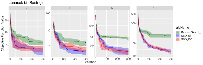
(a) BBOB Function 3 - Separable Rastrigin

(b) BBOB Function 13 - Sharp Ridge

Figure 1. Convergence plots of - and - on two of the 24 BBOB functions. Random search added as baseline. The experiments are run (from left to right) on 2,3,5, and 10 input-dimensions. The $y$-axis shows the best so far achieved objective function value on a logarithmic scale. The center line indicates the median of the algorithm repeats. The surrounding ribbon marks the lower and upper quartiles. $Y$-values measure differences from the global function optimum.

Our first set of results is presented in the form of convergence plots shown in Figure 1. The figure shows the convergence of the - and - algorithm on two of the 24 BBOB functions. These two functions (Rastrigin, Sharp Ridge) were chosen because they nicely represent the main characteristics and problems that can be observed for both infill criteria. These characteristics will be explained in detail in the following paragraphs. A simple random search algorithm was included as a baseline comparison. The convergence plots of all remaining functions are available as supplementary material, also included are the results with the R-package ‘mlrmbo’.

As expected, the random search is largely outperformed on three to ten-dimensional function instances. In the two-dimensional instances, the random search approaches the performance of -, at least for longer algorithm runtimes. For both functions shown in Figure 1, it can be observed that - works as good or even better than - on the two-, and three-dimensional function instances. As dimensionality increases, - gradually starts to overtake and then outperform -.

Initially, - seems to have a faster convergence speed on both functions. Yet, this speedup comes at the cost of being more prone to getting stuck in local optima or sub-optimal regions. This problem is most obvious in the two- and three-dimensional instances, especially on the two-dimensional instance of BBOB function 3 (Separable Rastrigin). Here, - shows a similar convergence to - on roughly the first 40 iterations. However, after just 100 iterations, the algorithm appears to get stuck in local optima, reporting only minimal or no progress at all. As Rastrigin is a highly multi-modal function, the results for - are not too surprising. At the same time, - yields steady progress over all 300 iterations, exceeding the performance of -.

Yet, this promising performance seems to change on higher dimensional functions. On the five- and ten-dimensional function sets, the performance of - is close to the one of - early on. Later in the run, - outperforms - noticeably. Neither algorithm shows a similar form of stagnation as was visible for - in the lower dimensional test scenarios.

This behavior indicates that with increasing dimensionality, it is less likely for to get stuck in local optima. Therefore, the importance of exploration diminishes with increasing problem dimension. De Ath et al. reach a similar conclusion for the higher dimensional functions they considered  (DeAt19a). They argue that the comparatively small accuracy that the surrogates can achieve on high dimensional functions results in some internal exploration even for the strictly exploitative -. This is due to the fact that the estimated location for the function optimum might be far away from the true optimum. In Section LABEL:sec:caseStudy this is covered in more detail. There, we investigate exactly how much exploration is done by each infill criterion.

3.2. Statistical Analysis

To provide the reader with as much information as possible in a brief format, the rest of this section will present data that was aggregated via a statistical analysis. We do not expect that our data is normal distributed. For example, we know that we have a fixed lower bound on our performance values. Also, our data is likely heteroscedastic (i.e., group variances are not equal). Hence, common parametric test procedures that assume homoscedastic (equal variance), normal distributed data may be unsuited.

Therefore, we apply non-parametric tests that make less assumptions about the underlying data, as suggested by Derrac et al. (Derr11a). We chose the Wilcoxon test, also known as Mann-Whitney test (Holl14a), and use the test implementation from the base-R package ‘stats’. Statistical significance is accepted if the corresponding p-values are smaller than $\alpha=0.05$. The statistical test is applied to the results of each iteration of the given algorithms. As the BBOB suite reports results in exponentially increasing intervals, the plot in Figure 2 follows the same exponential scale on the x-axis. The figure shows the aggregated results of all tests on all functions and iterations. Blue cells indicate that - significantly outperformed -, while red indicates the opposite result. Uncolored cells indicate that there was no evidence for a statistically significant difference between the two competing algorithms. The figure is further split by the input dimensionality (2,3,5,10) of the respective function, which is indicated on the right-hand side of each subplot.

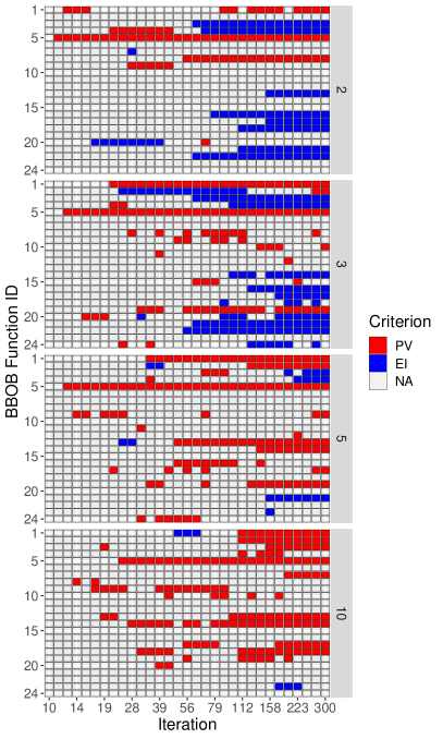
Figure 2. Statistical analysis of difference in performance between - vs. -. Y-Axis shows the BBOB-function index. Colors indicate which infill criterion performed better in each case, based on the statistical test procedure. Blank boxes indicates that there was no significant difference found. The results are presented for the 2,3,5 and 10 dimensional BBOB-function set as indicated in the gray bar to the right of each plot segment. The BBOB suite reports results in exponentially increasing intervals, thus the figure follows the same exponential scale on the x-axis.

We start with an overview of the two-dimensional results. Initially,