Optical spectroscopy of type-2 LINERs

Abstract

Context. Type-2 Low-ionization Narrow Emission-line Regions (LINERs) have been optically classified with the Palomar data as not presenting a broad component in the Balmer emission lines which is associated to the Broad Line Region (BLR) of the Active Galactic Nuclei (AGN).

Aims. We aim to unveil the presence of different kinematic components of emission lines in the nuclear region of a sample of local (z $\leq$ 0.022) type-2 LINERs. We focus on the analysis of the true nature of LINERs by means of the detection (or not) of a broad component originated in the BLR of the AGN. Additionally, we search for the possible presence of non-rotational motions such as outflows in these LINERs.

Methods. We have applied a decomposition of the nuclear emission lines using an spectroscopic analysis of the optical spectra of 9 type-2 LINERs of intermediate-resolution spectroscopic data retrieved from the Hubble Space Telescope (HST) archive. The study is completed with archival spectra from the Double Spectrograph from the Palomar Observatory.

Results. The emission line fitting reveals the presence of a broad component associated to the BLR in 6 out of the 9 galaxies for the space-based data, and for 2 out of the 8 from the ground-based spectra. The velocity dispersion for two galaxies (NGC 4486 and NGC 4594) measured in HST/STIS data suggest the presence of outflows.

Conclusions. The results indicate that the spatial resolution plays a major role in the detection of the BLR, as it appears diluted in the ground-based data (even after removing stellar contribution). This is also true for the emission line diagnostics, as the contaminant light contributes to lower emission line ratios toward the star-forming area of standard BPTs. We propose to reclassify NGC 4594 as a type-1 LINER, since a BLR component is seen in both space- and ground-based spectra. We find ambiguous results for the BLR component of NGC 4486. The modest outflow detection in our sample may indicate that they are not be as frequent as seen for type-1 LINERs.

1 Introduction

Low-ionization Narrow Emission-line Regions (LINERs) are among the lowest-luminosity active galactic nuclei (AGN) found in the Universe. Defined for the first time by Heckman (1980), their spectra is dominated by low-ionization lines in contrast to the importance of high-ionization emission lines ([O III]$\lambda 5007$ or He II$\lambda 4686$) in more luminous AGNs, as Seyferts. The initial separation between LINERs and Seyferts was defined by Heckman (1980) based on the relative ratios between the intensity of several emission lines ([O II]$\lambda 3727$ to [O III]$\lambda 5007$ and [O I]$\lambda 6300$ to [O III]$\lambda 5007$).

LINERs may be the most numerous type of AGNs in the local Universe (Ho et al., 1997), although their true AGN nature is still a matter of debate (Ho, 2008; Márquez et al., 2017). Their spectral features cannot be explained only with stellar formation processes (Heckman, 1980), but an AGN is not the only valid explanation. Other mechanisms that could reproduce their spectral features are, for example, shock ionization (Heckman, 1980; Dopita & Sutherland, 1995; Dopita et al., 1996) and photoionization by post-AGB stars (Binette et al., 1994; Stasińska et al., 2008; Papaderos et al., 2013).

The morphology of the circumnuclear H$\alpha$ emission as seen by the HST imaging indicates the possible presence of outflowing material in some of the systems (Pogge et al., 2000; Masegosa et al., 2011). In these cases, the outflow could contribute to the broadening of emission lines such as H$\alpha$-[N II], [O I] and [S II]. This could compromise the detection of the weak emission of Balmer lines from the Broad Line Region (BLR) in their nucleus. Shocks associated to outflows may be important also in ionizing the nuclear (and its surroundings) gas (Dopita et al., 1996; Molina et al., 2018). However, these are observed at lower velocities (Molina et al., 2018) than those needed by the shocks models (Groves et al., 2004) to reproduce LINER-like line ratios.

As Seyfert galaxies, LINERs appear as type-1.9 or type-2, depending on if the BLR is detected on their nucleus. The BLR is identified as a very broad component in the profiles of the Balmer lines. There are only a few systematic works studying the AGN nature of LINERs (Ho et al., 2003; Cazzoli et al., 2018), being most of them individual discoveries (Bower et al., 1996; Ho et al., 1997).

In the work by Cazzoli et al. (2018), the spectra for a sample of nearby (z $<$ 0.025) type-1.9 LINERs obtained with both ground- and space-based telescopes are analyzed. A broad component indicative of the BLR is required for the fitting of ground-based data in only a third of the targets, despite they where all classified as type-1.9 by Ho et al. (1997). Nevertheless, the modeling of the spectra of the targets obtained with the Space Telescope Imaging Spectrograph (STIS), mounted on the Hubble Space Telescope (HST), require a broad H$\alpha$ feature.

As in type-2 LINERs the BLR is not detected, the AGN nature of these systems is still controversial. Other components, as post-AGB stars or low mass X-ray binaries may play an important role to explain their optical spectra (see Ho et al., 1997; McKernan et al., 2010).

In this paper we analyze HST spectra of 9 type-2 LINERs selected from the sample of González-Martín et al. (2009) with available data in the archive to investigate if they present a broad component in the Balmer lines that could be associated to the existence of a BLR in their nuclei. We have completed the study by comparing with the ground-based spectra from Ho et al. (1995), since the majority of the targets have been classified as type-2 objects on that work. We also revisited the possible influence of the outflows in the broadening of Balmer lines, following Cazzoli et al. (2018).

This paper is organized as follows. In Section 2 we describe the sample and the data reduction process. Section 3 indicates the spectral line fitting for each nuclear spectra. Section 4 and Section 5 shows the main modeling results for space- and ground-based spectra, respectively. In Section 6 we discuss the modeling results, the possible presence of a BLR in some of the targets, and a comparison of the two data-sets for both kinematics and line ratios. Finally, in Section 7 we present a summary and the main conclusions of the work.

2 Sample and data processing

The sample selection is drawn from the survey by González-Martín et al. (2009) of 82 LINERs selected at X-rays. From this sample, we selected all type-2 LINERs classified as AGNs from the analysis of their features in the wavelength range from X-rays to the near-infrared. The final sample of 12 galaxies comprises all the objects with available spectra in the HST/STIS archive with the intermediate resolution grating G750M (R $\sim$ 5000).

This grating covers a total wavelength range from 5450 - 10140Å, centered at 6581 or 6768 Å. This range has been chosen due to the availability of the [SII]$\lambda\lambda$6716,6731Å; [NII]$\lambda\lambda$6548,6584Å; and H$\alpha\lambda$6563Å  lines in all the spectra and [OI]$\lambda\lambda$6300,6364Å  in those where the grating was centered at 6581Å (all except NGC 4594 and NGC 4676B). Two out of 12 were discarded because the low signal-to-noise ratio (S / N) of the spectra (NGC 4261 and NGC 5055, for which Constantin et al. 2015 already reported the poor quality of the nuclear spectrum of the latter), and also NGC 6240, because even though its spectrum is archived as to be nuclear, the emission lines were not visible. This leaves with a total of 9 galaxies in the final sample of type-2 LINERs. Their basic information is provided in Table 1.

The full calibrated 2D spectra were retrieved from the HST archive. In Table 2 the main observing details of each nuclear spectrum analyzed are listed. Then we extracted the 1D flux and wavelength -calibrated nuclear spectra of the sources. Some of them (namely NGC 4698, NGC 4552, NGC 4676B) showed abundant cosmic rays (CR). The results can be improved by performing a new CR correction with the L.A. Cosmic algorithm (van Dokkum, 2001) to the flat-fielded frames downloaded also from the archive. After this correction, we applied the last step of the reduction process following the HST pipeline, which is the x2d task (under the stsdas package in IRAF). This task generates the final calibrated frame and corrects for the geometrical distortion.

For the galaxies with several nuclear exposures available, they were realigned and combined with the IRAF tasks imshift and imcombine. These tasks improved the S/N after the CR rejection. If there was only one nuclear spectrum available and the CRs fell close to the lines in the majority of the nuclear rows, we extracted each row individually and did the CR removal manually. Then the individual rows were combined to form the final nuclear spectra. If a CR fell on the continuum of these spectra, it was masked in the analysis.

The final nuclear spectrum was extracted using apall task in IRAF. The number of extracted and combined rows depends on the slit width and the binning of the CCD. The majority of the targets were measured with a slit width of 52$\arcsec$ $\times$ 0.2$\arcsec$, a plate scale of 0.05$\arcsec$ pixel^-1 and no binning. For these, the 5 central rows (pixels) were extracted to form the final spectra. For the spectra binned to 0.1$\arcsec$pixel^-1, the 3 central rows were extracted. All the galaxies observed with a slit width of 52$\arcsec$ $\times$ 0.1$\arcsec$ were unbinned, and therefore we extracted 5 rows. The number of pixels extracted for each galaxy and its equivalent spatial scale are indicated in Table 2 (column 6).

However the data for two of the objects (NGC 4552 and NGC 4676B) had low S/N that did not improve with the combination of multiple exposures. As for NGC 4552 there were additional spectra from regions near the very center, a line-fitting was possible for the nuclear spectrum (see Sect. 3). We also fitted the NGC 4676B spectrum, but it was finally excluded due to the low significance of the obtained modeling, as will be discussed in Section 6.

Additionally, we searched for the spectra of the 9 objects within the sample by Ho et al. (1995) in order to compare the space-based and ground-based spectra. These latter were retrieved from the archival. They were observed with the Double Spectrograph (Oke & Gunn, 1982), located in the Cassegrain focus of the Hale 5 meter telescope at Palomar Observatory during 1984 and 1985. The long-slit spectra were measured with a 1200 line mm^-1 grating blazed to cover a wavelength range $\sim 6210-6860$Å . The spectral resolution was R $\sim$ 2500 for a 2$\arcsec$-length slit and R $\sim$ 4000 for a 1$\arcsec$-length slit. Spectra for 8 out of the 9 galaxies (all except NGC 4676B, member of a merging system, which is located at approximately 10 times the distance of the rest of the targets, see Table 1) were retrieved from the NASA/IPAC Extragalactic Database (NED) archive already reduced. The width of the slit was 2$\arcsec\times$128$\arcsec$ for all the targets except for NGC 4486 that was 1$\arcsec\times$128$\arcsec$. The total extraction window was 2$\arcsec\times$4$\arcsec$ (for NGC 4486 was 1$\arcsec\times$4$\arcsec$), equivalent to summing up the central 7 pixels of the CCD. The mean seeing of the observations is 1.5$\arcsec$. The spectral and spatial resolution was $\sim$2.5Å  and 0.58$\arcsec$ pix^-1, respectively.

Table 1: General properties for the 9 type-2 LINERs discussed in this paper. (2) ‘RA’and (3) ‘DEC’: coordinates of the galaxy; (4) ‘Morphology’: Hubble classification; (5) ‘z’and (6) ‘scale’: heliocentric redshifts and scale distance from the Local Group from NED; (7) ‘i’: inclination angle from Ho et al. (1997); (8) ‘V_rot’  and (9) ‘P.A.’: respectively, maximum rotation velocity corrected from inclination and position angle from HyperLeda.

ID	RA	DEC	Morphology	z	Scale	i	Vrot	P.A.
	(hh:mm:ss)	(dd:mm:ss)			(pc arcsec-1)	(∘)	(km s-1)	(∘)
(1)	(2)	(3)	(4)	(5)	(6)	(7)	(8)	(9)
NGC 2685	08 55 34.71	+58 44 03.83	(R)SB0+pec(a)	0.0029	70	60	146$\pm$4	38
NGC 3245	10 27 18.387	+28 30 26.79	SA(r)0(b)	0.0045	90	58	-	177
NGC 4374	12 25 03.74	+12 53 13.14	E1(c)	0.0034	65	-	189$\pm$15	135
NGC 4486	12 30 49.42	12 23 28.04	E0+pec(d)	0.0043	84	-	-	160
NGC 4552	12 35 39.81	+12 33 22.83	E(a)	0.0011	17	-	-	-
NGC 4594	12 39 59.43	-11 37 22.99	SA(s)a(a)	0.0034	59	68	408$\pm$11	90
NGC 4676B	12 46 11.24	+30 43 21.87	SB(s)0/a+pec(a)	0.0220	472	-	397$\pm$31	-
NGC 4698	12 48 22.91	+08 29 14.58	SA(s)ab(a)	0.0034	64	53	518	203$\pm$3
NGC 4736	12 50 53.061	+41 07 13.65	(R)SA(r)ab(a)	0.0010	25	36	182$\pm$5	105

^(a)Ho et al. (1997); ^(b)Wardle & Knapp (1986); ^(c)Huchtmeier (1994); ^(d)Huchtmeier & Richter (1986).

Table 2: Observing log of HST/STIS data. Columns indicate: (1) galaxy name; (2) other name; (3) filename of the analyzed spectra as indicated in the archive; (4) proposal ID of the observations; (5) position angle of the slit (north-eastward); (6) extraction window and its corresponding scale in parsecs; (7) date of the observation; (8) exposure time of the spectra; (9) filter used for the sharp-divided image (Márquez & Moles, 1996) obtained also from the HST archive. These latter are shown in Appendix B.

ID	Other name	Filename	Proposal	PA	Extr. window	Obs. date	Exp.Time	Im.Filter
		(_sx2 /_x2d)	ID	(∘)	pix (pc)	(yy-mm-dd)	(s)
(1)	(2)	(3)	(4)	(5)	(6)	(7)	(8)	(9)
NGC2685*	IRAS 08517+5855	o63n01020	$8607$	54	3 (21)	2001-05-06	$3097$	F814W
NGC3245	IRAS 10245+2845	o57205030	$7403$	203	5 (23)	1999-02-02	$2715$	F547M
NGC4374	M 84	o3wn01010/2010	$7124$	104	5 (17)	1997-04-14	$1993/2223$	F814W
NGC4486	M 87	o67z01010/2010	$8666$	164	5 (21)	2001-03-25/27	$1360$	F606W
NGC4552	M 89	o5l203020	$8472$	78	5 (4)	2000-06-19	$1440$	F555W
NGC4594	M 104	o4d303030	$7354$	250	5 (15)	1999-02-05	$280$	F814W
NGC4676B*	IC 820	o67q09030	$8669$	195	3 (144)	2002-02-20	$740$	F814W
NGC4698	IRAS 12458+0845	o4e022010/20/30	$7361$	259	5 (16)	1997-11-24	$900/933/840$	F606W
NGC4736	M 94	o67110030	$8591$	50	5 (6)	2002-07-15	$1440$	F555W

3 Analysis of the nuclear spectra

The host galaxy contribution on the nuclear spectra of a low-luminosity AGN may be significant, hence the starlight should be subtracted to robustly measure the kinematics and fluxes of the emission lines. However, due to the small wavelength range covered for the HST/STIS data (572 Å), we decided not to perform the subtraction as the line free continuum regions of the spectra are small for a proper stellar continuum modeling. Moreover, Constantin et al. (2015) (hereafter C15) proved that the correction is negligible for HST/STIS spectra in this wavelength range due to the small aperture of the instrument, that reduces the contaminant starlight from the host galaxy.

The starlight was modeled and subtracted for the Palomar data using a penalized PiXel fitting analysis (ppxf version 4.71 Cappellari & Emsellem, 2004; Cappellari, 2017). This differs to the stellar modeling applied by Ho et al. (1993), in which template galaxies were used instead (see Sect. 5.2). The methodology of the stellar subtraction was done following a similar technique as in Cazzoli et al. (2018) (hereafter C18). Similarly for the modeling of the spectral emission lines, which is explained in below. For each object, the restframe velocity used in the analysis is defined as: c $\times$ z (column 5, Table 1). The starlight decontamination for the Palomar data and all the line modelings to the different spectra are found in Appendices A and B, respectively.

3.1 Emission line fitting

Each of the emission lines present in the spectra ([S II], [N II], H$\alpha$ and in some cases [O I], Table LABEL:T_kin column 4) were fitted with Gaussian functions to derive their properties: central wavelength, line width ($\sigma$) and full-width half maximum (FWHM), flux and f_blend, defined as the percentage of the broad component flux with respect to the total flux of the H$\alpha$-[N II] lines. The fitting was performed using a non-linear least-squares minimization and curve-fitting routine (lmfit) implemented in Python, which is an extension of the Levenberg-Marquardt method found in the scipy package.

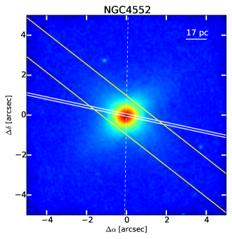
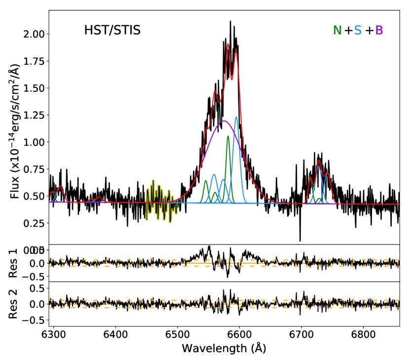
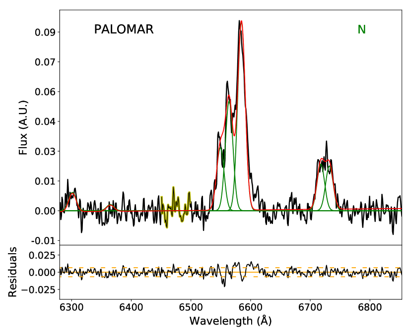
Figure 16: (General description in Appendix B). NGC 4552: For the HST/STIS spectrum, a second and a broad component were necessary to model emission lines. [O I] lines are very noisy and weak, thus they could not be used as a template for forbidden lines and narrow H$\alpha$. A broad component is not required to fit the H$\alpha$ profile. On the contrary, for the Palomar spectrum all the emission lines can be reproduced with only a single component.

The modeling of the lines was performed with three different methods using either [SII] or [OI] or both as templates for the H$\alpha$-[N II] complex (Cazzoli et al. 2018 and references therein). As H$\alpha$ and [N II] lines are generally blended, we do not use them directly because the overall fit could be affected. Among those emission lines available, the best lines are the [O I] lines as they are separated enough between them to be good templates. However, these lines are not always available or have low S/N (e.g. see Fig. 16), so we have to rely on [S II] lines, as done in previous works (Ho et al., 1997; Balmaverde & Capetti, 2014; Constantin et al., 2015). Therefore, the three different models we can apply are the use of [S II], [O I] or both (if available) as the reference lines because they are usually not strongly blended as H$\alpha$-[N II].

Following Cazzoli et al. (2018), the first method is called S-method, and consists on fitting the [S II] lines and then tie to them the central wavelengths and widths of all the other narrow lines. The second method (O-method) is the same as S-method but using as reference the [O I] lines. The third model is a mixed-model (M-model), that uses simultaneously both [S II] and [O I] lines as a template for the H$\alpha$-[N II] blend.

We tested different methods of fitting since the forbidden lines ions of the spectra have different critical densities ([S II] $\sim 10^{3}$ cm^-3, [O I] $\sim 10^{6}$ cm^-3 and [N II] $\sim 10^{4}$ cm^-3, respectively) caused by the possible stratification in the NLR. Therefore the profiles of each line could be different (see Balmaverde & Capetti 2014).

The fluxes of the two [N II] lines and the two [O I] lines were set to follow the relations 1:3 and 1:2.96, respectively (Osterbrock & Ferland, 2006). For more details on the methods and the constraints, we refer to C18.

As in C18 in order to prevent over fitting we calculated a parameter, $\varepsilon_{\rm c}$, which is the standard deviation of a region of the continuum that did not have any absorption or emission line. This parameter was always calculated in a 50Å -length region of the spectra. We compared it with the standard deviation of the residuals under each emission line and if $\varepsilon^{\rm line}$ $<$ 3 $\times$ $\varepsilon_{\rm c}$, then the fit is considered to be reliable. For the cases where $\varepsilon_{\rm c}$ was not sufficient in order to differentiate between two different fits, we used the $\chi^{2}$ of the fit and/or visual inspection as the last criteria to select the final model.

The procedure was organized in three steps. First, we fitted the continuum to a linear least-squares model using the regions between the emission lines visible in the spectra.

Second, all lines were fitted to a single Gaussian profile (hereafter ‘narrow component’) with the same parameters for all of them. If the fit was satisfactory for the reference lines ([S II] or [O I]) but not for [N II] and H$\alpha$, then a broad Gaussian profile was added to H$\alpha$ (hereafter ‘broad component’). However, if the fit was not reliable in any of the lines or if the narrow component had a large velocity ($\geq$ 300 km s^-1), then a second component was added to all the lines (hereafter ‘secondary component’).

Third, if the H$\alpha$-[N II] blend is not well reproduced (significant residuals) with a narrow plus a secondary component, then we added a broad component in H$\alpha$. All the line modelings are presented in the figures of the Appendix B.

This method was not sufficient for the most complicated cases, for which additional restrictions were required. For example, the modeling of the reference lines for the NGC 4594 HST/STIS spectrum was good enough, but the maximum of the profiles of [N II] and H$\alpha$ seemed to be shifted ($\sim$1 - 3 Å) from the maximum of the Gaussian profiles. Thus we shifted 1Å the maximum of the secondary Gaussian component to improve the fit. This produced a change in the velocity compatible within the initial error estimation.

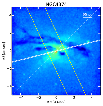
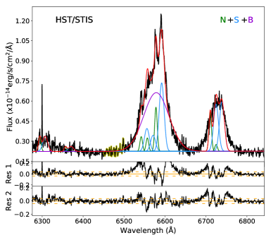
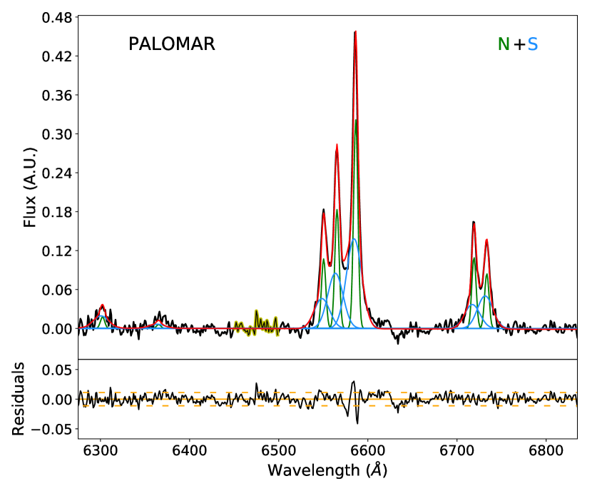
Figure 14: (General description in Appendix B). NGC 4374: In the HST/STIS spectrum, [S II] lines are severely blended and only the [O I]$\lambda$6300Å  line is visible (with low S/N). This complicated the modeling for the other lines, so the fit was performed considering the narrow peaks of [N II]-H$\alpha$ blend (see Sect. 3), which results in high residuals under the [S II] lines. A broad component is needed in this decomposition. For the Palomar spectrum, all the emission lines are well modeled with two Gaussian components.

For the HST/STIS spectra of two galaxies (namely NGC 4374 and NGC 4552) the [S II] lines were so blended and the [O I] lines almost absent, that it was challenging to perform the modeling using them as reference (Fig. 14 and 16). Thus we decided to fit the spectrum of a region situated a few pixels away from the nucleus and use this result to model the narrow component of the nuclear region. This was motivated by the assumption that the narrow component is tracing the kinematics of the disc of the galaxy, thus it should also be visible in regions outside the very center of the system. Moreover, by moving to an outer part of the galaxy, the contribution of the BLR (if present) should disappear due to its unresolved nature at HST scale. As the disc should be rotating with the same velocity dispersion, then a modeling of this component in the spectra of an outer region would give approximately the same contribution that we should expect in the nucleus, but with a shift in velocity. We note though that for some galaxies this condition is not completely true, as the disk velocity dispersion was found to increase towards the center (for NGC 3245 and NGC 4594 see Barth et al., 2001; Emsellem & Ferruit, 2000, respectively). This is discussed in more detail for each individual case in Sect. 6.3.2.

An additional assumption was made for NGC 4374. If the narrow component was fixed as within the previous method, when proceeding with the rest of the modeling the secondary component was broad enough to be compatible with a very broad AGN component of $\sigma>$ 800 km/s. The addition of a third Gaussian in the H$\alpha$-[N II] complex generated instead a narrow profile to fit a peak that is visible in the spectrum (see Fig. 14). Thus we exchanged the secondary and broad components to improve the fit.

We fixed the velocity dispersion of the narrow component for NGC 4374 and NGC 4552 with this method, and allowed the velocity to vary in the nuclear spectra. This improved the final residuals and visually with respect to the normal fitting process.

The velocities, V, and line widths, $\sigma_{\rm line}$, obtained for each galaxy, as well as the number of components and the model used to fit the reference lines are indicated in Table LABEL:T_kin. The S-method was used for all cases except for the Palomar spectrum of NGC 4552, for which we used the O-method. The line width has been corrected from the instrumental width by doing $\sigma_{\rm line}=\sqrt{\sigma_{\rm obs}^{2}-\sigma_{\rm inst}^{2}}$, where the value of $\sigma_{\rm inst}$ ($\sim$1.34 Å) has been taken from the HST/STIS handbook, and from Ho et al. (2009) for the Palomar data ($\sim$2.2 Å).

4 Modeling of HST/STIS data

Table 3: Results from the analysis of the optical spectra. From left to right: ‘ID’: object designation; ‘Inst.’: HST/STIS or Palomar spectra; ‘Comp.’: components used for the best-fitting model with N, S and B referring to narrow, second and broad components, respectively; ‘[O I]’: if these lines are present in the spectrum or not (Yes/No); velocity (V) and velocity dispersion ($\sigma$) for each component for each of the reference emission lines; ‘f_blend’: contribution of the broad component to the total flux of the H$\alpha$-[N II] complex.

ID	Inst.	Comp.	[O I]	V${}_{\rm N}^{\rm[S\,II]}$	$\sigma_{\rm N}^{\rm[S\,II]}$	V${}_{\rm S}^{\rm[S\,II]}$	$\sigma_{\rm S}^{\rm[S\,II]}$	V${}_{\rm B}^{\rm H\alpha}$	$\sigma_{\rm B}^{\rm H\alpha}$	fblend
				(km s-1)	(km s-1)	(km s-1)	(km s-1)	(km s-1)	(km s-1)	(%)
(1)	(2)	(3)	(4)	(5)	(6)	(7)	(8)	(9)	(10)	(11)
NGC 2685	HST/STIS	N	N	80 $\pm$ 1	63 $\pm$ 12	-	-	-	-	-
	Palomar	N	Y	-10 $\pm$ 1	70 $\pm$ 10	-	-	-	-	-
NGC 3245	HST/STIS	N + B	N	134 $\pm$ 29	172 $\pm$ 6	-	-	424 $\pm$ 12	998 $\pm$ 6	47
	Palomar	N + S	Y	-216 $\pm$ 9	25 $\pm$ 40	94 $\pm$ 17	136 $\pm$ 21	-	-	-
NGC 4374	HST/STIS	N + S + B	Y	-275 $\pm$ 13	146 $\pm$ 14	362 $\pm$ 5	281 $\pm$ 24	693 $\pm$ 7	1432 $\pm$ 37	65
	Palomar	N + S	Y	117 $\pm$ 4	51 $\pm$ 29	33 $\pm$ 56	395 $\pm$ 71	-	-	-
NGC 4486	HST/STIS	N + S	Y	395 $\pm$ 4	198 $\pm$ 22	-101 $\pm$ 378	655 $\pm$ 18	-	-	-
	Palomar∗	N + S + B	Y	-478 $\pm$ 4	238 $\pm$ 5	96 $\pm$ 6	286 $\pm$ 9	-285 $\pm$ 145	908 $\pm$ 141	5
NGC 4552†‡	HST/STIS‡	N + S + B	Y	-103 $\pm$ 47	157 $\pm$ 18	501 $\pm$ 38	249 $\pm$ 50	541 $\pm$ 53	1360 $\pm$ 20	70
	Palomar†	N	Y	56 $\pm$ 59	282 $\pm$ 68	-	-	-	-	-
NGC 4594	HST/STIS	N + S + B	N	70 $\pm$ 15	108 $\pm$ 26	66 $\pm$ 152	554 $\pm$ 6	519 $\pm$ 120	1677 $\pm$ 18	16
	Palomar	N + B	Y	-11 $\pm$ 4	215 $\pm$ 7	-	-	698 $\pm$ 26	956 $\pm$ 41	33
NGC 4676B∗‡	HST/STIS‡	N + B	N	527 $\pm$ 40	198 $\pm$ 12	-	-	336 $\pm$ 16	748 $\pm$ 12	89
NGC 4698	HST/STIS	N + B	N	55 $\pm$ 19	90 $\pm$ 5	-	-	273 $\pm$ 97	1375 $\pm$ 9	39
	Palomar	N	Y	-7 $\pm$ 2	98 $\pm$ 8	-	-	-	-	-
NGC 4736	HST/STIS	N + B	Y	127 $\pm$ 14	84 $\pm$ 12	-	-	330 $\pm$ 1	738 $\pm$ 4	82
	Palomar	N	Y	23 $\pm$ 4	105 $\pm$ 10	-	-	-	-	-

4.1 Overall modeling summary

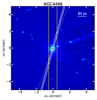
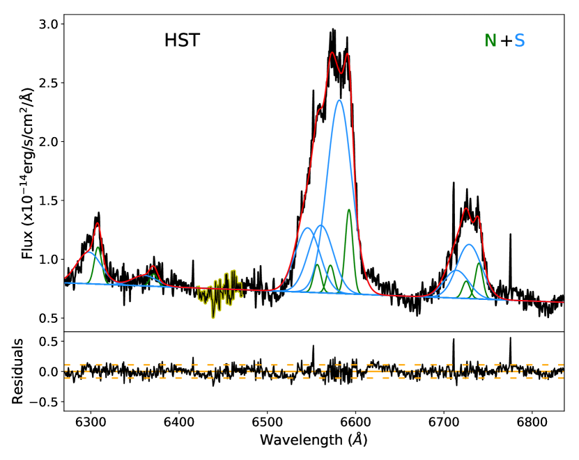
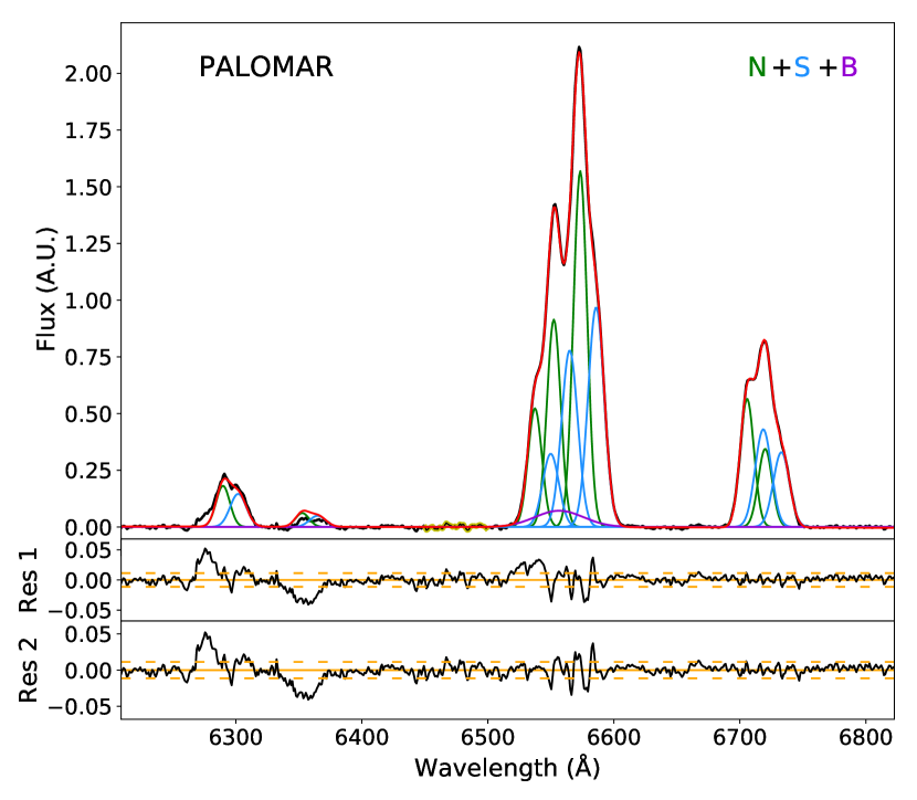
Figure 15: (General description in Appendix B). NGC 4486: In the HST/STIS spectrum, two components are required to model the broad [O I] and [S II] emission. No broad component is needed to model the H$\alpha$ line profile. For the Palomar spectrum, two components have been used to reproduce the [S II] and [O I] lines, but a very faint broad component is used for H$\alpha$.

Despite there were three possible models to fit the lines, we have selected the S-method to model all the HST/STIS spectra for different reasons. For 5 LINERs the spectrum was lacking the [O I] lines either for the wavelength range coverage or because they were not detected (Table LABEL:T_kin column 4). For two LINERs, NGC 4374 and NGC 4552, the S / N of the [O I] lines was rather faint and difficult to model (see Sect. 3.1). For NGC 4736, the fit presented no significant difference when applying S-/O-/M-models, so we decided to use the simplest model that could explain the observed spectra, in this case, the S-model. For the remaining object, NGC 4486, although one of the [O I] lines is clearly visible (Fig. 15), the modeling was better with the S-method (the $\chi^{2}$ improved about $\sim$30%). All the fits to the different spectra can be found in the Appendix B.

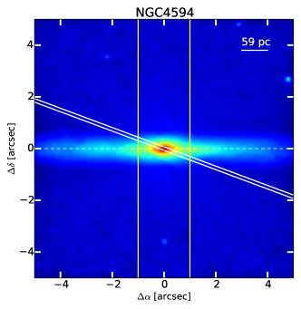
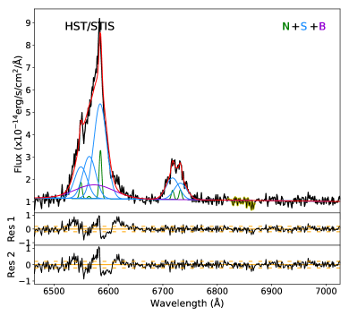
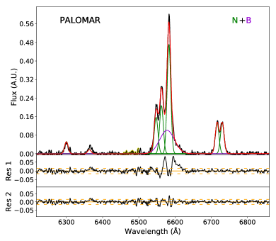
Figure 17: (General description in Appendix B). NGC 4594: The wavelength coverage of HST/STIS spectrum does not include [O I] lines. The [S II] lines have separate narrow profile peaks and a broader profile underneath. A broad component for H$\alpha$ is to improve the fit. This broad component is also needed for the Palomar spectrum, although a single narrow Gaussian is sufficient for the forbidden lines.

Generally, the modeling of both [S II] and [O I] lines are inside the 3$\varepsilon_{\rm line}$ limits for all LINERs except for NGC 4374 (see Fig 14). However, in the case of [N II] - H$\alpha$, $\varepsilon_{\rm c}$ is approximately equal to 3$\varepsilon_{\rm line}$ for NGC 4594 and $\sim$ 4$\varepsilon_{\rm line}$ for NGC 4374 despite the addition of the very broad component (Fig 17). In all the other objects, $\varepsilon_{\rm c}$ is within 3$\varepsilon_{\rm line}$ limits, thus we consider the fit to be not well constrained for these 2 cases.

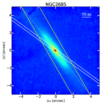
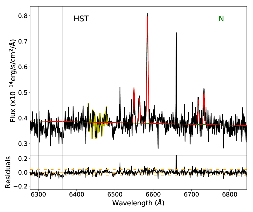
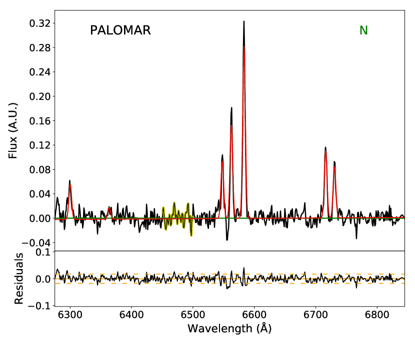
Figure 12: (General description in Appendix B). NGC 2685: The H$\alpha$-[NII] lines are unblended in both spectra. [O I] lines are not present in the HST/STIS spectrum, thus [S II] lines were used to model the other profiles. In the Palomar spectrum [O I] lines are visible, however no significant improvement was seen by using them to model the rest of the emission lines. All the lines are well reproduced with a single narrow Gaussian component.

We find that NGC 2685 is the only spectrum that can be modeled with a single narrow component in all the emission lines and NGC 4486 is the only spectrum well reproduced with a narrow plus a secondary component. No very broad component is required for them (Fig. 12 and 15). For the other 7 LINERs we found that 4 out of 9 need one narrow Gaussian component to model all the forbidden lines and an additional broad (BLR) component in H$\alpha$ (see Table LABEL:T_kin column 3). On the other hand, the remaining 3 LINERs need a secondary component to model the forbidden lines and narrow H$\alpha$ in addition to a very broad component in H$\alpha$.

In summary, a secondary component is needed in 4 out of the 9 analyzed galaxies and a very broad component in H$\alpha$ is needed in 7 out of the 9 LINERs.

4.2 Comparison with Constantin et al. 2015 (C15)

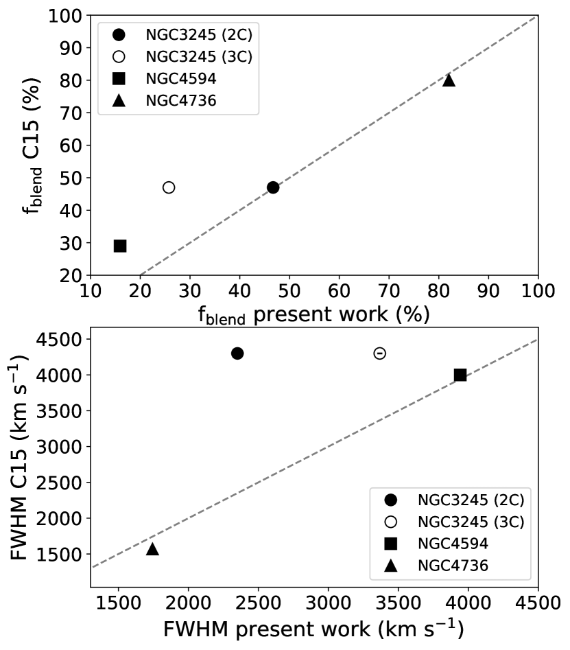
Figure 1: Comparison of the contribution in percentage of the broad component of H${\alpha}$ to the total flux of the H${\alpha}$-[N II] complex (upper panel) and the FWHM of the very broad component (lower panel) derived in this work versus C15. Each symbol represents a different LINER as indicated in the legend. The filled (empty) circle represents the two-(three-)component fit to NGC 3245. The gray-dashed line is the one-to-one comparison.

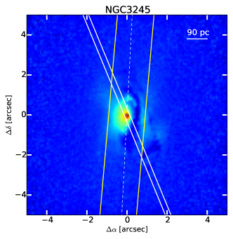
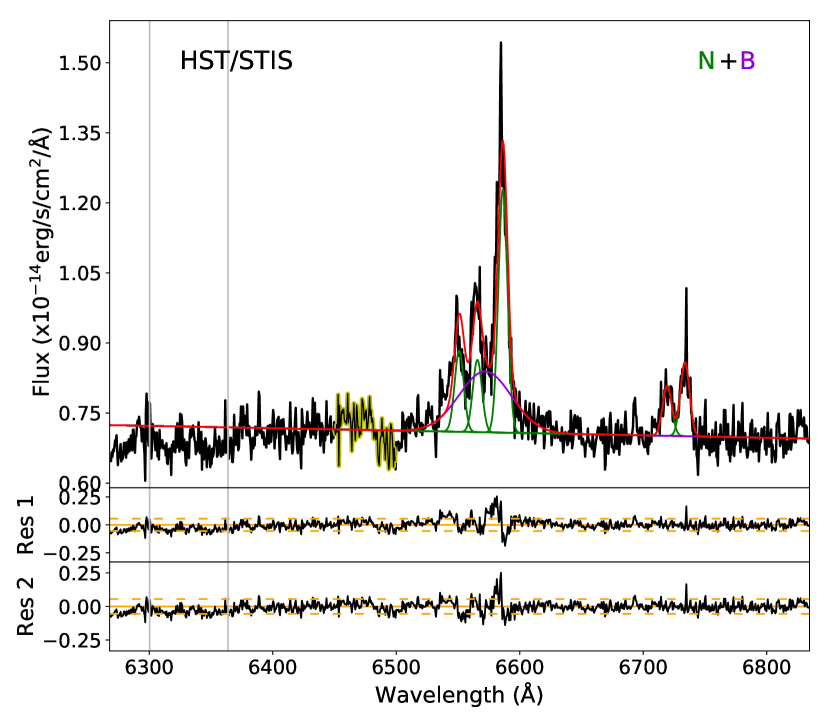
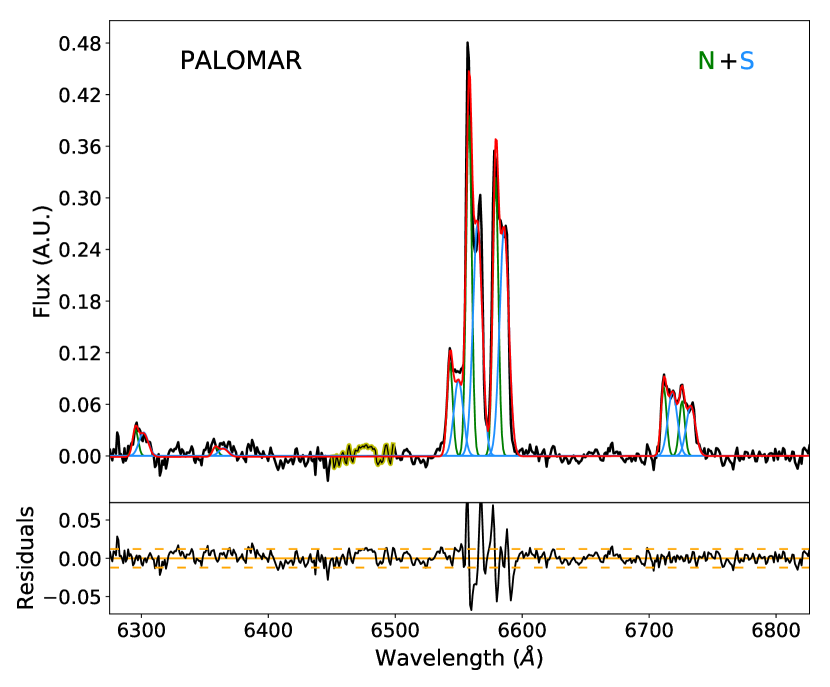
Figure 13: (General description in Appendix B). NGC 3245: For the HST/STIS spectrum, the emission lines have been modeled with a single narrow Gaussian component. The residuals improved by adding a broad component to H$\alpha$. [O I] lines are not visible. In the Palomar spectrum, the double-peaked line profiles are modeled with two Gaussian components. As the [O I] line is rather faint, [S II] lines have been used for the modeling. H$\alpha$ does not require any BLR-originated component.

Most of the galaxies shown here (7 out of 9; 77% of the sample) have already been analyzed by C15, where they report for the first time the detection of broad components in 8 objects of their total sample. They have studied a total of 113 AGNs with HST/STIS and MMT (Multiple Mirror Telescope) spectroscopic data to analyze the emission lines and to give constraints on the ionizing mechanisms present in the galaxies. The reduction process of the HST/STIS data and the line modeling, for which they used the [S II] lines as template for the H$\alpha$-[N II] blend, follow a similar technique to us. For the galaxies in common, they found a broad H$\alpha$ emission for three of them (NGC 3245, NGC 4594, NGC 4736) in agreement with our findings (see Table LABEL:T_kin and Fig. 13, 17 and 20).

A direct comparison of the contributions of the very broad component to the H${\alpha}$-[N II] complex and the FWHM for these 3 galaxies can be seen in Fig. 1. NGC 3245 is represented with an empty or filled symbol depending on the number of components used for the modeling. Fig. 1 shows that, although if we consider our two-component modeling the contribution of the very broad component to the H$\alpha$ - [N II] complex is compatible in both analyses, the FWHM is more similar in the case of the three-component fit. The reason for this could be a direct consequence of the number of components. If we have two Gaussians for each emission line plus a broad component, its contribution to the global fit is going to be smaller than for a modeling of a single Gaussian plus a broad component, as the total flux of H$\alpha$ - [N II] is going to be distributed among more components.

The number of components for the modeling of NGC 4594 and NGC 4736 is the same as C15 (see Table LABEL:T_kin; Fig. 17, 20), thus no more additional models were considered. In both cases the results are in agreement with C15, although these authors indicate that the very broad component of NGC 4594 is very difficult to interpret (see Sect. 6.3.2). This very broad component dominates over the narrow to the H$\alpha$ line flux in both analyses, as can be seen in Fig. 17. The broad component for NGC 4736 contributes significantly to the total flux of both H${\alpha}$ and the whole H${\alpha}$-[N II] complex, as can be seen in Fig. 1.

For three galaxies (NGC 4374, NGC 4552 and NGC 4698; Fig. 14, 16, 19, respectively) we derive a very broad component ($>$ 1300 km s^-1) that C15 do not report in their analysis. According to our modeling, the fit is improved in the three galaxies by adding a very broad H$\alpha$ component to the H$\alpha$-[N II] complex. These detections are individually discussed in Sect. 6.3.2.

5 Modeling of Palomar data

5.1 Overall modeling summary

The Palomar data was analyzed by Ho et al. (1997) (hereafter H97) also looking for the possible presence of a very broad component in the spectra. We have analyzed 8 galaxies of their sample by testing all the three different fitting methods as described in Section 3. This is possible for the ground-based data-set, as the [O I] lines are visible in all cases (Table LABEL:T_kin, column 4; see figures in Appendix B).

The best fitting is obtained with the S-method for nearly all the spectra (7 out of 8), as no significant improvement was seen when using the other methods. NGC 4552 was the only galaxy for which we selected the O-method due to the severe blending of the [S II] lines (see Fig. 16).

We find that 4 galaxies (NGC 2685, NGC 4552, NGC 4698 and NGC 4736) can be modeled with a single narrow component in all the emission lines and 3 galaxies (NGC 3245, NGC 4374 and NGC 4486) need a narrow plus a secondary component, with NGC 4486 requiring a very broad component to obtain a proper model of the spectrum (see Sect. 6.3.1). NGC 4594 is the only case whose spectrum is modeled with a narrow Gaussian component for all the forbidden lines and an additional broad H$\alpha$ component (see Fig. 17). In summary, a very broad component in H$\alpha$ is needed in 2 out of the 8 galaxies and a secondary component is needed in 3 out of the 8 LINERs (see Table LABEL:T_kin).

5.2 Comparison with Ho et al. 1997 (H97)

In the search for broad emission lines done by H97, they analyzed the data of the galaxies from Ho et al. (1995) whose line profiles showed (or at least hinted) the presence of a broad H$\alpha$ emission. This reduced the total sample from 486 to 211 galaxies, from which only in 34 objects this broad feature was detected. The possible existence of a broad component in eight of the common objects is discussed below.

The methodology used in H97 to analyze the spectra consisted on an initial stellar subtraction using the spectra of galaxies devoid of emission lines (i.e. ‘template-galaxies method’, Ho et al. 1993 and references therein) and then a line modeling. C18 also tested the ‘template-galaxies method’, although when applying the ppxf routine to the spectra of the templates (see Sect. 3), some weak emission lines were visible in 6 out of the 10 template galaxies. Thus, we used the ppxf method instead of the ‘template-galaxies method’, as they need to be treated very carefully in order to avoid the inclusion of emission lines produced by the interstellar medium (see C18 for further details).

The line modeling in H97 consisted on a single Gaussian fit to the [S II] lines, considering them as reference to model the H$\alpha$-[N II] lines. Similar to our methodology, an additional broad component could be added to the H$\alpha$ line only when necessary (see Sect. 3.1).

The spectra modeling for 4 of the galaxies (NGC 3245, NGC 4486, NGC 4594 and NGC 4698) is shown in H97. Three of them (namely NGC 4552, NGC 4594 and NGC 4698) are among their null detection of a broad component, whereas NGC 2685, NGC 3245 and NGC 4486 are among the ambiguous cases. For these, according to H97, the cause of ambiguity is the template chosen for the starlight subtraction.

In our analysis, thanks to the use of ppxf, we minimized possible source of ambiguity related to the stellar modeling and subtraction (see Sect. 3 and C18). In our modeling for these same spectra, we find a broad component in 2 out of the 8 common objects (NGC 4486 and NGC 4594). Only for NGC 4594 this broad component is also visible on the HST/STIS spectra (see Fig. 17). This result indicates that the two objects, or at least NGC 4594, could have been initially classified as type-1 LINERs also with ground-based spectroscopy using a different starlight decontamination method and a different line modeling. For the other galaxy, NGC 4486, the existence of a broad component has been a matter of debate in previous works with both ground- and space-based spectroscopy (e.g. Harms et al., 1994; Ho et al., 1997; Walsh et al., 2013; Constantin et al., 2015, see Sect. 6.3.1). It was described in H97 as showing weak wings at either side of [N II] lines. Although when adding a broad component to the fitting their residuals improve, they say that this component could be a product of some ambiguities with the modeling, so they decided not to include it in the analysis. Its contribution to the global fit is rather weak (5%), but we also improve the residuals from our fitting by including it (Fig.B4) . We discuss its presence or absence in our ground and space data in Sect. 6.4.

6 Results and Discussion

We note that, given the difference among the slit-widths between Palomar and HST/STIS data (see Sect. 3.1), we will consider the latter results as the most accurate in characterizing the innermost parts of the AGN. Hence, the following kinematical analysis is only focused on them. Apart from this, the possible discrepancies between the measured narrow-component velocities from ground- to space-based data (see Table LABEL:T_kin) may be produced by the different alignment of the slits.

6.1 Overall summary of kinematics

The wavelength-shift and line-width of each of the Gaussian components used to model the spectra are converted into a measurement of velocity and velocity dispersion of the ionized gas kinematics. We can associate them to a kinematic component of the galaxy. To this aim, we have followed the velocity-velocity dispersion (V-$\sigma$) classification similar to that used in C18, which is shown in Fig. 2.

This figure is divided into 4 different regions, associated to rotation, outflows, inflows and candidates for rotational motions. Dividing limits of the regions have been established by C18 by measuring the gas velocity field from the 2D spectra of the type-1.9 LINERs within their sample, and estimating the maximum broadening of the emission lines associated to rotational motions. The C18 conservative upper limit for this component is $\sim$400 km s^-1, although the typical values of velocity dispersion ($\sim$200 km s^-1) in their sample is well below this limits (see Sect. 5.2 in C18). This limits are supported by the fact that the ionized gas in rotation usually produces a broadening of the lines that is traduced into velocity amplitudes up to $\sim$300 km s^-1 (see e.g. Cappellari et al., 2007; Epinat et al., 2010). They found that the regions outside the nuclear zone in the 2D spectra had amplitudes $\sim$300 - 400 km s^-1, thus associating this part of the V-$\sigma$ diagram to candidates for broadening produced by rotational motions.

As for the velocities, typically the narrow component of type-1.9 LINERs has values $\pm$50 km s^-1. Thus, when the $\sigma$ is larger than 300 km s^-1, these broadening cannot be addressed to rotational motions but instead to non-rotational motions. Then we would consider them as candidates to the presence of outflows or inflows. For the intermediate cases, the targets are considered as candidates for non rotational motions.

For the secondary component, C18 found that the velocity dispersion present typically values from 400 to 800 km s^-1. In this case, the broadening is probably related to turbulent non-rotational motions. It is seen in Fig. 2 that the velocities for the secondary component of type-1.9 LINERs present typical values ranging from -200 $\leq$ V${}_{S}\leq$ 100 km s^-1 (see C18). For this analysis we have decided to apply similar limits to C18 because the complete study of the gas velocity field could not be done with the present data-set. Thus, it has to be noted that the region limits could be different for type-2 LINERs if a similar analysis is considered. However, the physical interpretation of the position in the diagram for the galaxies with a secondary component is unlikely to change dramatically given their large velocity dispersion $>$500 km s^-1 and hence their position on Fig. 2.

6.2 Classification of the velocity components

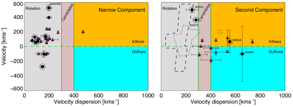
Figure 2: Velocity dispersion versus velocity derived for the narrow (left panel) and secondary (right panel) components used to model the HST/STIS spectra for both type-1.9 from C18 (red triangles) and type-2 (black filled circles) LINERs. An additional black circle marks those cases for which a broad component is needed in HST/STIS spectra. All type-1.9 LINERs from C18 show a broad component. Each of the marked regions indicate to which kinematic component can be associated the modeled component. The orange region indicates inflows, blue region indicates outflows, pink region indicates candidates for both inflows and outflows, and the gray region indicates rotation. On the right panel, the contours of the narrow components are shown for both type-1.9 (dotted lines) and type-2 (dashed lines) LINERs.

As mentioned in the previous section, if the velocity dispersion is in the range up to 300 km s^-1, the component may be associated to the presence of a rotating disc in the galaxy. The broad H$\alpha$ component is not considered in this figure as it is interpreted unequivocally as a manifestation of the BLR of the AGN. The narrow component, present in all the ground- and space-based spectra, shows velocity dispersions consistent with being produced by rotation. On the other hand, the secondary component is always broader than the narrow, and has a higher spread on the velocity dispersion for both type-1.9 and type-2 LINERs, with typical values higher than $\sim$ 400 km s^-1. These values are consistent with the presence of non-rotational motions (outflows or inflows).

In Fig. 2, only four galaxies of the HST/STIS sample (NGC 4374, NGC 4486, NGC 4552 and NGC 4594) needed a secondary component on the line modeling. From these, only for NGC 4374 and NGC 4486 a second component is added in the Palomar spectra. NGC 4486 and NGC 4594 line widths of the secondary component are consistent with being caused by the presence of non-rotational motions, which is also suggested by previous results (e.g. the H$\alpha$ morphology of NGC 4486 shown in Masegosa et al., 2011). For the remaining cases, the line widths are compatible with being produced by rotational motions, although NGC 4374 could be a possible inflow candidate. Also in Masegosa et al. (2011) the possible presence of an outflow seen with the H$\alpha$ emission was discarded (or inconclusive) for this galaxy due to the dust lanes that obscure and limit the access to the nuclear H$\alpha$ morphology. For NGC 4552, a bipolar nuclear outflow was reported by Machacek et al. (2006) with Chandra images (0.5 - 2 keV).

The other galaxy in the sample which has been previously reported as hosting an outflow is NGC 3245. The H$\alpha$ image of this galaxy shows an unresolved nucleus and a structure indicative of the presence of an outflow (Masegosa et al., 2011), which is also supported by the kinematic analysis of (Walsh et al., 2008). However, in our modeling of the HST/STIS spectrum, a secondary component is not needed (see Sect. 6.3.1) and, if used, the resulting velocity and velocity dispersion will be compatible with being caused by rotation (V${}_{\rm s}=-40\pm 25$ km s^-1; $\sigma_{\rm s}=194\pm 56$ km s^-1). With the Palomar data instead, a secondary component is clearly required to satisfactorily reproduce the line profiles with low residuals (Fig. 13). In this case, the secondary component also has a velocity and velocity dispersion in agreement with rotation, so it is not clear that it could be associated to non-rotational motions.

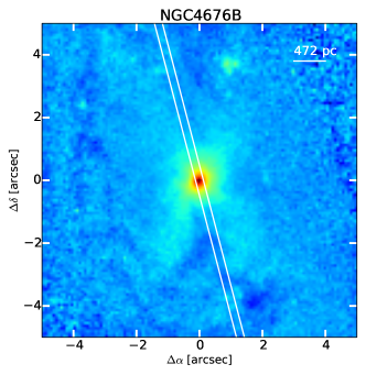
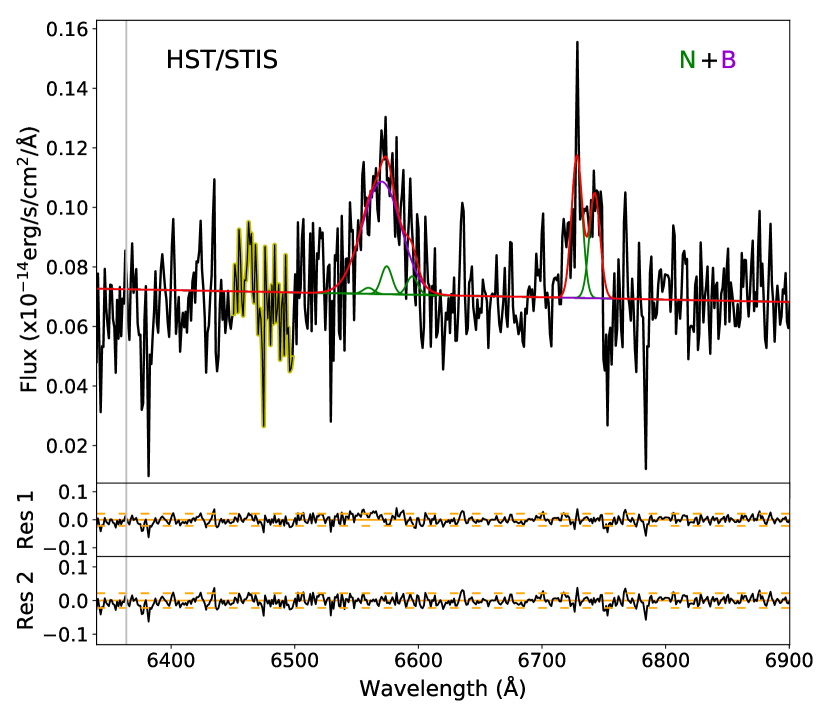
Figure 18: (General description in Appendix B). NGC 4676B: The S / N of the HST/STIS spectrum is generally low and the quality of the fitting could be hampered. Both this and the wavelength range starting at 6340 Å  make the [O I] lines not visible, so only the S-method could be applied. The fit slightly improves by adding a broad component. There is no Palomar spectra for this galaxy. The PA is not indicated as this galaxy belongs to an interacting system and there is no clear determination of it.

We can directly compare our values with the results from the HST/STIS analysis of 12 type-1.9 LINERs from C18. It is clearly seen that the narrow component for both samples can be explained by rotational motions (see Fig. 2). The typical values of velocities and velocity dispersion (see Sect. 6.1) are similar except for some cases. NGC 4676B has a velocity higher than 500 km s^-1. It is a merging galaxy, and its modeling is not well constrained (see Fig. 18 and Sect. 6.3). In Wild et al. (2014) they quote a big velocity gradient oriented in a similar direction to where the HST/STIS slit is allocated, which may suggest that the velocity of the narrow component could be affected by this. NGC 4374 and NGC 4486 have larger velocities of the narrow component than what should be expected (see Sect. 6.1). For the latter also Noel-Storr et al. (2003) found that the narrow component was not rest frame in the central spectrum. For the first, they might be produced by the large velocity gradients present in the innermost parts and that we are not considering individually in this analysis (see Sect. 6.3.2). On the other hand, the values for the secondary component are more spread throughout the diagram, including 2 galaxies in the range in which the broadening could be explained by rotation. Velocities for the secondary component of type-1.9 LINERs are more concentrated than type-2 LINERs, with values ranging from -110 $\leq$ V_S $\leq$ 500 km s^-1 for the latter. The velocity dispersion range is more similar for both samples, ranging from 250 $\leq$ V_S $\leq$ 800 km s^-1. The proportion of objects within the C18 sample that present a secondary component is slightly higher than that of type-2 LINERs (7 out of 11 versus 4 out of 9). This result could be a consequence of the orientation of the slit, that could not capture the full extension of putative outflows or inflows. However, this comparison could be not completely representative of these populations due to the modest amount of type-2 LINERs in the sample.

6.3 Individual comments for the galaxies

This section is organized taking into account the components used to fit the HST/STIS spectra, as indicated in Table LABEL:T_kin (column 3). The figures with the spectra modeling are in Appendix B. As in all cases the BLR components in our analysis have large velocity shifts, we have tried to set the velocity of the BLR-component to zero in order to statistically confirm its true velocity. The majority of the models presented worse residuals both visually and statistically (i.e. difference in $\chi^{2}>15$% worse) than with the final velocities (see Table LABEL:T_kin). We discuss individually the results for the galaxies that did not change much with this model.

6.3.1 Model with only narrow components

As mentioned in Sect. 4, we have been able to model only two of the galaxies (NGC 2685 and NGC 4486) with a narrow or a narrow plus a secondary component (see Table LABEL:T_kin).

The HST/STIS spectra of NGC 2685 has been analyzed in two works. González Delgado et al. (2004) compare the main ionizing mechanism of this LINER measured with both ground- and space-based instruments, although the data-set for STIS use the G430L grating. It is the only galaxy in their analysis that requires a single narrow Gaussian component to reproduce the observed spectrum. C15 applied exactly the same modeling for the same data-set using only narrow components. Hence, our results are consistent with previous ones.

For NGC 4486 is a complex galaxy with a well-known radio jet. Noel-Storr et al. (2003) analyzed this spectrum in first place and found that the presence of a broad component improved visually and statistically the global fit of the spectrum with respect to a single Gaussian component per line. The velocity of the narrow component they measure in the central pixel is $\sim$ 260 km s^-1. Neither Walsh et al. (2013) nor C15 found a broad H$\alpha$ component when modeling the emission lines. Walsh et al. (2013) reports the existence of velocity gradients in the innermost regions of the slit, as for the case of NGC 4374 (see Sect. 6.3.2). The velocity dispersion can be as high as 600 km s^-1 in the central row, and it decays in the following regions. In our case, this structure is integrated in our spectrum. Our fit does not improve significantly by adding a very broad component to a two component fitting (only a 5%), thus only two components were used. In this case, the secondary component is consistent with an outflow (see Table LABEL:T_kin and Fig. 2). However, a second component with large width could be also the result of the strong gradient in the velocity dispersion reported by Walsh et al. (2013). For the Palomar spectrum, a broad component improves a 18% the fit, although the $\varepsilon_{\rm c}$ was already smaller than 3$\varepsilon_{\rm line}$ (see the residuals of the fit without the broad component in Fig. 15). Given this and the non-clear detection in previous works, we should consider the (non) detection in the Palomar (HST/STIS) spectrum as ambiguous. The non-detection of the HST/STIS data implies that this component, if existing, should not be attributed to typical BLR clouds orbiting nearby the black hole but instead to other phenomena on larger scales (e.g. inflows/outflows).

6.3.2 Models with broad BLR-originated component

The remaining 7 galaxies were found to require a very broad component with the emission-line fitting analysis.

NGC 3245 was classified as an intermediate case between a LINER and a transition object (Ho et al., 1997). HST/STIS data was analyzed in first place by Barth et al. (2001), who studied the dynamics of the ionized gas in this galaxy. They suggested the possible presence of a broad component in H$\alpha$, which was modeled by C15 (see Sect. 4.2). Their emission line modeling consisted on 3 Gaussian profiles fitted to [N II] - H$\alpha$ lines (tied in velocity but allowed to vary in $\sigma$). In our case, visual inspection indicates that only one narrow component is sufficient to fit the lines, although with a secondary component the $\chi^{2}$ of the fit improves approximately a 16%. We have prioritized the simplest model that is able to describe the observed spectrum (S-method; see Fig. 13). In either case, a broad component in H$\alpha$ was necessary to model the line profiles.

The spectrum of NGC 4594 obtained with the TIGER 3D spectrograph shows some irregularities in its nucleus and a strong velocity gradient ($\sim$300 km s^-1) near the center (Emsellem & Ferruit, 2000). However, as neither the HST or Palomar slits are located along the major kinematic axis of the galaxy (see Fig. 17), we would not expect a strong line-broadening due to the ordinary disk rotation. The H$\alpha$ emission is concentrated in the spiral arms and in the nuclear region of the galaxy (Masegosa et al., 2011). There has been some debate about the presence of a broad H$\alpha$ component in the spectra of this galaxy. There are studies supporting both its presence (Kormendy et al., 1996; Walsh et al., 2008) and its absence (Ho et al., 1997; Nicholson et al., 1998). Hence a methodology that takes into account all the different possibilities, as the one presented in this work, is required to understand the true nature of this LINER-nucleus. The spectrum presents wings in the H$\alpha$ - [N II] lines that was initially attributed to the existence of a BLR with data from the HST/Faint Object spectrograph (Nicholson et al., 1998). On the one-to-one row analysis by Walsh et al. (2008), they show that there are large velocity gradients in the nuclear regions covered by the HST/STIS slit. These gradients could be producing the observed line-profile, as indicated in Sect. 3.1. The best fit to the HST/STIS spectrum is obtained with two components plus a broad component, as C15 (see Sect. 4.2 and Fig. 17). The residuals are still higher than 3$\varepsilon_{line}$, they have been reduced from 3.2 to 2.7 for [N II]$\lambda$6548Å  and the $\chi^{2}$ of the overall fit is improved a 15% by adding the broad component. If we were to set the velocity of the BLR component to zero, the $\chi^{2}$ would be only a 3% worse and the $\sigma$ would be 10 km s^-1 less broad. However, as this component has a negligible flux contribution to the total H$\alpha$-[N II] blend and it is the broadest line we found in our study (see Table LABEL:T_kin), it should be expected to find no difference between both modelings statistically. However, visually the red wing of the [N II]6584$\AA$ line is better reproduced with the velocity as indicated in Table LABEL:T_kin. Hence, we decided to not set to zero the velocity of the broad H$\alpha$ component.

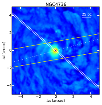
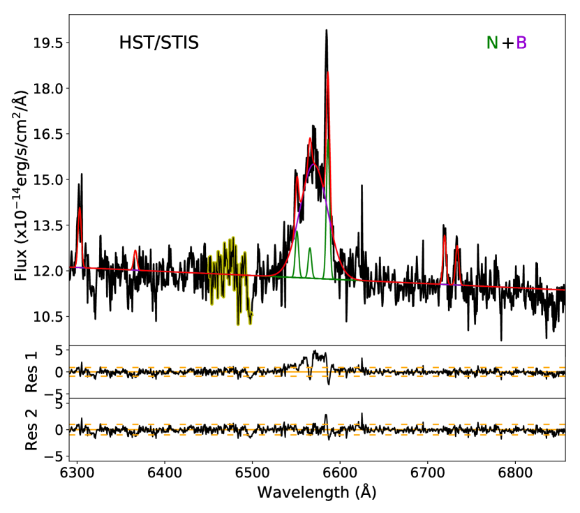
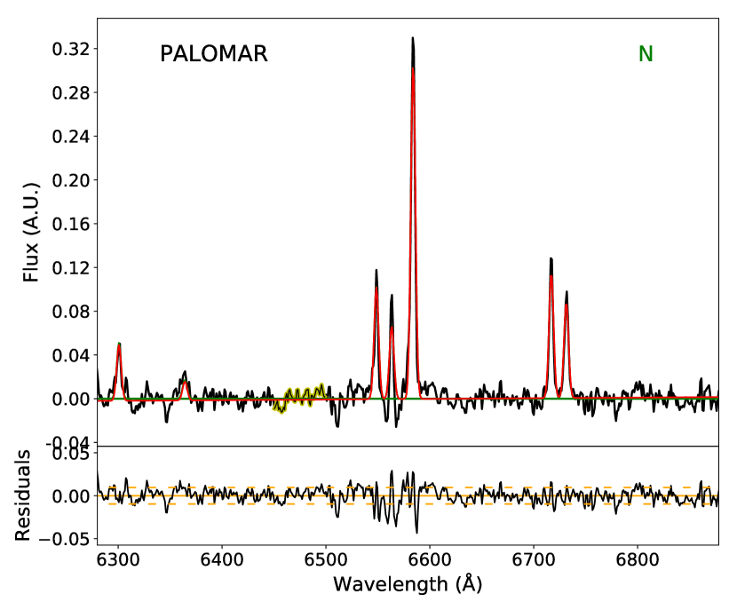
Figure 20: (General description in Appendix B). NGC 4736: Both [S II] and [O I] lines are unblended in the HST/STIS spectrum and they clearly present narrow profiles. In the H$\alpha$-[NII] lines a broad component is visible, as already reported by Constantin et al. (2015). For the Palomar spectrum a narrow component is sufficient for fitting all the emission lines considered in our study.

NGC 4736 is an interesting case as the broad component is clearly visible in the HST/STIS spectrum (Constantin & Seth, 2012, C15) but it has never been reported from ground-based observations (Ho et al., 1997; Constantin & Seth, 2012). The size of the slit-aperture is crucial in this object to classify it properly. The broad component has also been reported with a Principal Component Analysis (PCA) Tomography method applied to Integral Field Unit (IFU) data taken several years after the HST/STIS spectra (Steiner et al., 2009). In our analysis all the forbidden lines, except the H$\alpha$-[N II] complex, are well-modeled with a single narrow Gaussian component. For H$\alpha$ a broad component of $\sigma_{\rm B}\sim 740$ km s^-1 is needed (see Sect. 4.2 and Fig. 20). The FWHM of this component is in the limit of being associated with the BLR of the galaxy, which is also the case for NGC 4676B (see below). Both $\sigma_{\rm B}$ are only slightly higher ($\sim$100 km s^-1) that the $\sigma_{\rm S}$ for NGC 4486.

C15 did not report additional very broad detections for the other galaxies in common (NGC 2685, NGC 4374, NGC 4486 and NGC 4552; see Sect. 4.2). However in our analysis two of them present a very broad component, whereas the other two only need a narrow and a narrow plus a secondary component (NGC 2685 and NGC 4486, respectively), as indicated previously (see Sect. 6.3.1).

For the modeling of NGC 4374 and NGC 4552 nuclear spectra we have used a different technique from the rest of the galaxies. As explained in Sect. 3.1, in both cases the [O I] lines are barely detected, hence only the S-method could be applied but [S II] are severely blended.

The HST/STIS spectra of NGC 4374 were first analyzed by Bower et al. (1998) and a few years later by Walsh et al. (2010). In the former work, they used two Gaussian components to fit the lines, considering that they were tracing two dynamically different gas components, (a rotating disk and a low-velocity component unrelated to the disk). The latter showed that the profiles of [N II]-H$\alpha$ could be affected by the NLR kinematics, which is rapidly rotating, although their analysis do not exclude the presence of a broad component. As in the case of NGC 4594, the presence of a BLR-originated component is debated. In C15 they concluded that a broad component in H$\alpha$ was not needed (see Sect. 4.2). Nevertheless, its presence was not ruled out by Walsh et al. (2010) in the 3 innermost rows, where a peaked central velocity dispersion, associated to the emission-line disk, is related to large velocity gradients visible mainly in the central row of the slit (see Sect. 6.2). In our analysis, these gradients are integrated in the final spectrum as we do not perform a one-to-one row analysis (to maximize the S/N). In this sense, our narrow component fit should be properly considered as a lower limit to the velocity dispersion of the disk. Both narrow and secondary component are compatible with rotation (see Fig. 2 and Table LABEL:T_kin), which is somewhat expected from the results of Walsh et al. (2010). In this work, they do not show the values of the three nuclear rows analysis, as their kinematical profiles are said to be complicated to analyze due to the large gradients. However the amplitude of the velocities is comparable with that of the secondary component ($\sim$400 km s^-1), being coincident with assumed limit for detecting outflows (Sect. 6.2 and Fig. 2).

In the case of NGC 4552, Cappellari et al. (1999) modeled the emission lines with intermediate width profiles in both permitted and forbidden lines and highlighted the low luminosity of the central engine in comparison with others AGNs. With respect to the HST/STIS spectra, C15 do not consider a broad component. In our modeling, that take into account a second component in forbidden lines and narrow H$\alpha$, reveals the presence of a broad component in both galaxies that contributes significantly ($\sim$ 65% and $\sim$ 70%, respectively) to the global fit, as can be seen in Figures 14 and 16 (see Sect. 4.2).

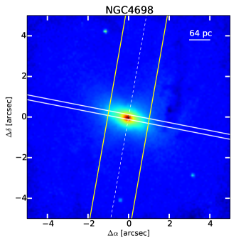
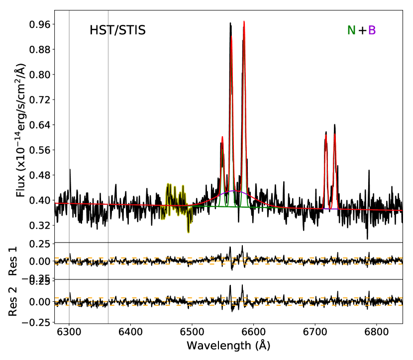
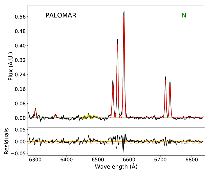
Figure 19: (General description in Appendix B). NGC 4698: [O I] lines are not visible in the HST/STIS spectrum. A narrow Gaussian component is sufficient to fit [S II] lines, and a broad component in H$\alpha$ to improve the modeling, although its contribution to the global fit is rather weak. For the Palomar data a single narrow component is sufficient to model the lines.

NGC 4698 data come from the Survey of Nearby Nuclei with STIS, known as SUNNS, analyzed by Shields et al. (2007). They suggest that the galaxy was badly classified as a type-2 Seyfert galaxy by Ho et al. (1997), on the basis of a decrease of the level of the excitation mechanism, suggesting that it is a LINER or a transition object. These authors did not detect a broad component in H$\alpha$ in their spectral analysis, as Balmaverde & Capetti (2013) and C15 when analyzing the same data-set in contrast to our finding. More specifically, we have found that, even though the [S II] lines are perfectly modeled with a single narrow component, the addition of a weak broad component improves the $\chi^{2}$ of the fit a $\sim$ 17% (see Fig. 19). The lack of detection of this component in previous works could be due to its low contribution to the global fit (39%, Table LABEL:T_kin) flux in comparison with the narrow component (see Sect. 4.2). If we were to set the velocity of the broad component to zero, we find that the $\chi^{2}$ of the fit would be only 0.5% worse than the fit with the velocity from Table LABEL:T_kin. As for NGC 4594, the broad component has a rather low contribution to the global flux and is the second broadest component in our analysis, thus again statistically we should expect a small difference. In this case, also visually there was no difference. However, due to the rather low velocity of this component in the previous model (273$\pm$97 km s^-1; Table LABEL:T_kin), we decided not to add any constrain on the broad component velocity.

The remaining galaxy, NGC 4676B, belongs to the Mice galaxies complex, two interacting spiral galaxies. Both spirals have been told to present features indicative of the presence of outflows (Masegosa et al., 2011; Wild et al., 2014). Its HST/STIS nuclear spectrum has not been studied before as the S/N is rather low, which makes it difficult to analyze (see Fig. 18). Despite this, we attempted to model the emission line, being the unique measurement of this kind for this object with HST/STIS data. Our fit has revealed the presence of a broad component for the H$\alpha$-N[ II] complex, while a narrow component is sufficient to fit the [S II] lines. Even though the $\chi^{2}$ improved with the addition of this component, the residuals are inside the 3$\varepsilon_{\rm line}$ limits also with a single narrow-modeling for all the lines. The presence of this component could be affected by the noise and the FWHM of this component is not as broad (748 km s^-1; Table LABEL:T_kin) as the other detections in our sample. The results of the test of setting the velocity of the broad component to a zero velocity show the same results in FWHM and $\varepsilon$-indicator. Then it is not clear if it can be associated to the presence of a BLR. To avoid possible ambiguities, in what follows we have conservatively excluded it as a true detection of a broad component.

6.4 BLR in optically classified type-2 LINERs?

Type-2 LINERs have been classified by optical, ground-based spectroscopy as not having a broad component in the Balmer emission lines while it is not the case for type 1-1.9 (Ho et al., 1993, 1995). Nevertheless we have seen in our analysis (Sect. 6.3) that 6 out of the 9 analyzed galaxies in our sample exhibit this component in space-based spectroscopy. In the case of the 22 type-1.9 LINERs (selected from the Palomar Sky Survey) all the available space-based spectrum (12 LINERS) showed a broad component in H$\alpha$ (C18 for details).

However, the same objects analyzed with the original Palomar spectra from Ho et al. (1997) do not show this feature except for 2 cases in type-2 LINERs (NGC 4486 and NGC 4594), and do show it in all except 4 cases in type-1.9 LINERs. Ho’s initial classification is mainly supported by this result. However, this enhances the difference of the ground-based spectra with those from space, based also on the results of C18.

The detection of a broad component is favored in space-based spectra because of the spatial resolution (Molina et al., 2018). If the BLR exists in a particular galaxy, a wider slit on a ground-based instrument could prevent it to be detected, as the weak broad H$\alpha$ component could be diluted. This could be the reason for the initial lack of detection of the BLR in the galaxies of our sample, but also the modeling of the lines (e.g. testing single and multiple components) could be crucial to highlight its presence (as it was our case for HST/STIS spectra of NGC 4374 and NGC 4552).

NGC 4486 is the only case in which the broad component is detected on the Palomar spectrum but not in the HST data. As we should expect exactly the opposite behavior (i.e. the detection of this component on HST and not in Palomar spectrum), it is not clear if this galaxy should be reclassified (type-1 instead of type-2). Moreover if we take into account that the existence of the BLR in this object has been largely discussed in the literature (see Sect. 5.2). On the other hand, NGC 4594 is the only object in which a very broad component is detected in both data-sets, so it should then be considered as a type-1 LINER.

6.5 Line ratios

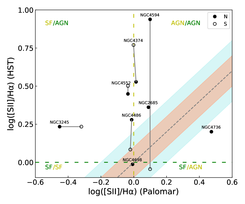
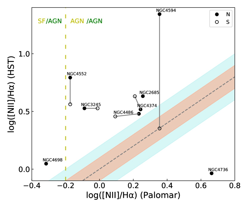
Figure 3: Comparison of the line ratios for [S II]/H$\alpha$ (top) and [N II]/H$\alpha$ (bottom) for both HST/STIS spectra (y-axis) and Palomar spectra (x-axis). The gray dashed line is the one-to-one comparison. Filled circles represent the narrow component whereas the empty circles are for the secondary, which is connected to the narrow through a gray solid line when present. The light pink and light blue ranges indicate the 10% and 20% uncertainty levels with respect to the one-to-one comparison, respectively. Green and yellow dashed lines indicate the limits (HST and Palomar, respectively) for the star-forming (SF) and AGN regions. The limits were obtained from Kauffmann et al. (2003) and Kewley et al. (2006).

We have analyzed the line ratios for the emission lines available in all spectra. In Figure 3 the [N II]/H$\alpha$ and [S II]/H$\alpha$ line ratios for both Palomar and HST data are shown. We have estimated the ratios for both the narrow and the secondary components (when present) for all galaxies except NGC 4676B, as its modeling is not well constrained (see Sect. 6.3).

We consider in Fig. 3 the empirically-derived separation between an AGN or a star forming (SF) system as in the BPT diagrams (Baldwin et al., 1981; Kauffmann et al., 2003; Kewley et al., 2006). Based only in [N II]/H$\alpha$ and [S II]/H$\alpha$ ratios. Since [O III]/H$\beta$ is not available in our data, we consider the star formation as the dominant mechanism of ionization if log([S II]/H$\alpha$) is $<0.0$. The mechanism would be the AGN ionization when log([S II]/H$\alpha$)$>0.0$. For the log([N II]/H$\alpha$), the limit for SF is $<-0.2$, for AGN $>0.2$, and ‘transition’ region elsewhere.

In general, evident differences are seen in both panels of Fig. 3 between the space- and ground-based data. For both [N II]/H$\alpha$ and [S II]/H$\alpha$, the ratios are always positive for the HST data, whereas more dispersion in the values exists in Palomar data (Palomar vs HST mean/standard deviation for [N II]/H$\alpha$ 0.15/0.30 vs 0.54/0.40; and [S II]/H$\alpha$ 0.02/0.24 vs 0.37/0.26). Specifically, for Palomar (HST) the average and standard deviation are for log([N II]/H$\alpha$) equal to 0.15 and 0.30 (0.54 and 0.40), respectively; for log([S II]/H$\alpha$) these values are 0.02 and 0.24 (0.37 and 0.26).

In absence of [O III]/H$\beta$ (see Sect. 2), the ratios are more compatible with the AGN region for the HST spectra than for the Palomar data. The difference could be due to the spatial resolution based on the recent results from Molina et al. (2018). They have analyzed 3 LINERs with HST data, and performed a detailed study about the line diagnostic diagrams considering the unresolved nuclear source and what they call an ‘integrated’  spectrum, that resembles the spectra of the targets as seen from a ground-based telescope. They found that the line ratios tend to be higher for the unresolved nuclear source than for the integrated spectrum. They conclude that it could be produced by the addition of a large spatial region of the galaxy ($\sim$100 pc) within the integrated spectrum, where there is influence from gas probably suffering simultaneously photoionization and shock effects. This is reflected on their line ratios being consistent with different ionization mechanisms.

In Fig. 3, NGC 2685, NGC 4698 and NGC 4736 only have a single narrow component (black circles), so they appear only once. The difference with respect to the one-to-one line could be explained directly with the variation of the H$\alpha$ profile seen in the HST with respect to the Palomar spectra (see Fig. 12, 19 and 20). Although, except for NGC 4698, they are compatible with being produced by an AGN in both Palomar and HST. For the case of NGC 4698 line ratios correspond to the transition region in both diagrams for the HST data, so this results in an ambiguous classification. The varying H$\alpha$ profile does not only produce considerable differences in the line ratios for these 3 objects, but also for NGC 3245 and NGC 4486 (see Fig. 13 and 15, respectively).

The differences in the H$\alpha$ profiles are important, but also there are dramatic variations for the ratios of the secondary with respect to the narrow component. The most extreme case is NGC 4594 (see Fig. 17 and Fig. 3), in which the H$\alpha$ contribution to the total flux of the narrow component is almost negligible in comparison to the contribution of the secondary and the broad component. However, the secondary component shows a very similar line ratios than for the Palomar spectrum.

In the top panel of Fig. 3, considering the [S II]/H$\alpha$ ratio, the great majority of points for ground-based data are located around the transition region (i.e. log([S II]/H$\alpha$)$\sim$0.0). In these cases, the information of the [O III]/H$\beta$ ratio is required to further constraint the source of the ionization field. This is true for all objects except for NGC 4736, which is the only galaxy for which both [N II]/H$\alpha$ and [S II]/H$\alpha$ line ratios of the narrow component are consistent with being produced by the AGN, as mentioned above. Our classification, based on the [S II]/H$\alpha$ ratio, is consistent with the presence of a very broad component (BLR-originated) visible in its HST spectrum (Fig. 20).

On the other hand, for the classification based on [N II]/H$\alpha$ ratio, the majority of objects (7 out of 8) fall within the AGN region and only one is consistent with being ionized by a SF region.

7 Summary and conclusions

In this work we present a kinematic analysis and the study of ionization mechanisms of the gas of 9 type-2 LINERs with both space- and ground-based spectroscopy obtained from the HST/STIS archive and from the Palomar/Double Spectrograph (Ho et al., 1995), respectively.

The main objective is the detection of the existence of a BLR in these galaxies by analyzing its spectral emission line features and the possible presence of outflows. Moreover, we addressed the line ratios of the emission lines to study the dominant ionization mechanism for these objects.

We used the [S II] and [O I] lines as templates to model the other forbidden lines ([N II]) and narrow H$\alpha$, and considered the addition of a broad component under H$\alpha$ when necessary. We used a maximum of 3 Gaussians component named narrow, secondary and broad component. Our approach allowed us to explore a larger number of scenarios for modeling emission lines with respect to previous work. These scenarios include possible NLR-statification and non-rotational motions being present, and never explored, for type-2 LINER-nuclei (see C18 for type-1 LINERs).

The narrow component is likely to be associated with the rotation from the galaxy disk, whereas the secondary component,of intermediate width, could be related to both rotational or non-rotational motions (as outflows). The broad component of the Balmer lines is always associated to the BLR of the AGN.

The secondary component has been detected for 4 LINERs in the HST spectra and for 3 in the Palomar data. For two objects from the HST analysis (i.e. NGC 4486 and NGC 4594), this component is found to suggestive of non rotational motions such as outflows. The line width of these components is similar to those found for outflows in type-1.9 LINERs by Cazzoli et al. (2018).

The detection of the BLR in LINERs is crucial to reveal its true AGN nature. Ho et al. (1997) optically classified 8 of the galaxies as type-2 objects, because their line fitting did not require a very broad component BLR-originated to reproduce the H$\alpha$-[N II] profile. With our analysis (following C18) of the same Palomar-spectra, we have found that for 2 out of 8 LINERs, a broad component is indeed necessary to reproduce emission lines. For the space-based data a very broad component is needed in 6 out of the 9 analyzed objects.

The only detection of this component in the Palomar data but not confirmed with the HST is for NGC 4486. The results for this component are not well constrained, thus we consider the BLR component detection as ambiguous. NGC 4594 is the only galaxy in the sample for which a broad component is needed in both space- and ground-based spectra, indicating that it would be better classified as as a type-1 LINER.

Three of the BLR detections in the HST data (NGC 3245, NGC 4594 and NGC 4736) were already reported by Constantin et al. (2015). Our measurements of both FWHM and flux contribution of the broad component with respect to the total flux of the H$\alpha$-[N II] complex agree with Constantin et al. (2015).

The detection of a very broad component is favored with the HST data as the spatial resolution is 10 times better than for the Palomar data, decreasing the amount of contaminant starlight from the host galaxy and preventing the possible dilution of the broad component. The spatial resolution could be also relevant for the line diagnostic diagrams, as the calculated line ratios vary significantly from ground- to space-based spectra.

Appendix A Stellar modeling and subtraction for Palomar spectra

The starlight modeling and subtraction to the ground-based spectra is presented here for the 8 available LINERs. The stellar continuum in the observed spectra was modeled with the ppxf method as in Cazzoli et al. (2018) (Sect. 3).

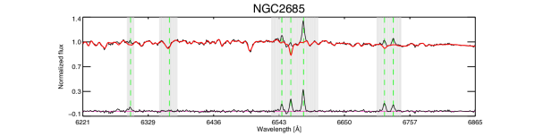
Figure 4: Optical ground-based Palomar spectrum of NGC 2685. The original data is shown in black; the red line indicates the modelled stellar spectrum that matches the observed stellar continuum. The spectrum used for the kinematical decomposition (i.e. data $-$ model) is also presented. Green dashed lines show the rest-frame position of the [O I], [N II]-H$\alpha$ and [S II] lines. Grey bands indicate the regions masked to perform the stellar modeling. The magenta line indicates the zero-level as reference.

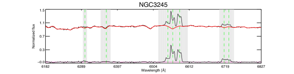
Figure 5: Same as Fig. 4 but for NGC 3245.

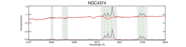
Figure 6: Same as Fig. 4 but for NGC 4374.

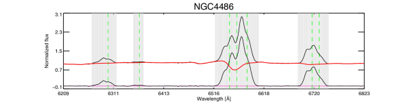
Figure 7: Same as Fig. 4 but for NGC 4486.

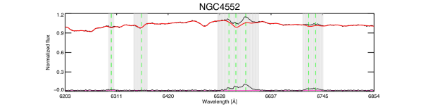
Figure 8: Same as Fig. 4 but for NGC 4552.

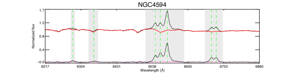
Figure 9: Same as Fig. 4 but for NGC 4594.

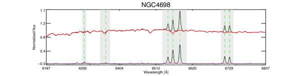
Figure 10: Same as Fig. 4 but for NGC 4698.

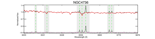
Figure 11: Same as Fig. 4 but for NGC 4736.

Appendix B Spectra modeling for each galaxy

We present HST images from the archive and the spectra analyzed in this manuscript for each LINER. They are arranged as follows.

• Top: sharp divided (Márquez & Moles 1996; Márquez et al. 1999, 2003) HST image of the galaxy in the inner 10${}^{{}^{\prime\prime}}$x10${}^{{}^{\prime\prime}}$. The HST filters are summarized in Table 2, column 9. Sharp-divided images are very useful to trace asymmetries in the light distribution, such as bars, spiral arms, dust lanes and rings. The method consists on dividing the original image by that obtained from the convolution with a median filter of 30 pixels. This technique allows the subtraction of the diffuse background emission facilitating the detection of small-scale variations and discuss the possible presence of both dust extinguished and more luminous regions (e.g. Masegosa et al. 2011). The galaxy ID is indicated in the panel title. White and yellow continuous lines represent the slit used to obtain the HST/STIS and Palomar spectrum (when available), respectively. The angular scale of 1″of the image in parsecs (see Table 1 column 6) is indicated in the right-upper part of the image. The white dashed line indicates the PA of the major axis (see Tab. 1).

• Middle: line modeling of the HST/STIS spectra (see Sect. 3 for details). We marked with different colors each Gaussian component (same colours mark the same kinematic components). Green lines represent the narrow component; when present, blue lines represent the secondary component and purple lines, the broad component. The red curve shows the total contribution of all the components. The continuum range selected to calculate the standard deviation is plotted in yellow. Residuals from the fits are in the middle/lower panels. We have included the residuals of the fit without the broad component for those objects in which this component was necessary (labeled as: ‘Res 1’) for comparison. When the two are plotted, the final fit residuals are labeled as: ‘Res  2’. In these panels, the orange lines indicate the 3$\sigma$ limits. If the [O I] lines are not present, their restframe position is indicated in gray in both spectrum and residual. Wavelengths are restframe.

• Bottom: line modeling for the Palomar data (same description as in previous panel) after stellar continuum modeling and subtraction (see Sect. 3 and Appendix A). The flux is in arbitrary units.