Estimating dust attenuation from galactic spectra. I. methodology and tests

Abstract

We develop a method to estimate the dust attenuation curve of galaxies from full spectral fitting of their optical spectra. Motivated from previous studies, we separate the small-scale features from the large-scale spectral shape, by performing a moving average method to both the observed spectrum and the simple stellar population model spectra. The intrinsic dust-free model spectrum is then derived by fitting the observed ratio of the small-scale to large-scale (S/L) components with the S/L ratios of the SSP models. The selective dust attenuation curve is then determined by comparing the observed spectrum with the dust-free model spectrum. One important advantage of this method is that the estimated dust attenuation curve is independent of the shape of theoretical dust attenuation curves. We have done a series of tests on a set of mock spectra covering wide ranges of stellar age and metallicity. We show that our method is able to recover the input dust attenuation curve accurately, although the accuracy depends slightly on signal-to-noise ratio of the spectra. We have applied our method to a number of edge-on galaxies with obvious dust lanes from the ongoing MaNGA survey, deriving their dust attenuation curves and $E(B-V)$ maps, as well as dust-free images in $g$, $r$, and $i$ bands. These galaxies show obvious dust lane features in their original images, which largely disappear after we have corrected the effect of dust attenuation. The vertical brightness profiles of these galaxies become axis-symmetric and can well be fitted by a simple model proposed for the disk vertical structure. Comparing the estimated dust attenuation curve with the three commonly-adopted model curves, we find that the Calzetti curve provides the best description of the estimated curves for the inner region of galaxies, while the Milky Way and SMC curves work better for the outer region.

1 Introduction

The observed spectrum of a galaxy is a combination of several components: a continuum, absorption and emission lines. The continuum and absorption lines are both dominated by starlight, thus usually referred to as the stellar component of the spectrum, while the emission-line component is produced in Hii regions around hot stars, or emission-line regions of active nuclei, or both. All these components, however, are modified by the attenuation of dust grains distributed in the inter-stellar space. Dust attenuation can affect galaxy spectra over a wide range of wavelengths, from ultraviolet (UV), optical to infrared, by absorbing short-wavelength photons in UV/optical and re-emitting photons in the infrared, and the absorption is stronger in shorter wavelength. Consequently, dust attenuation can cause changes in the overall shape of a galaxy spectrum. Such attenuation has to be taken into account before one can measure the different components of an observed spectrum reliably.

Various schemes have been used to estimate dust attenuation. For Milky Way and nearby galaxies, such as the Magellanic Clouds, observations of individual stars can directly probe the dust extinction along different lines of sight (e.g., Prevot et al., 1984; Cardelli et al., 1989; Fitzpatrick, 1999; Gordon et al., 2003). Far-infrared (FIR) observations provide direct measurements of dust attenuation for more distant galaxies because the emission by dust dominates the spectral energy distribution (SED) of FIR, although such observations can be made only through space telescopes. When both infrared (IR) and UV photometry are available, dust attenuation may be estimated by the IR-to-UV luminosity ratio, $\rm L_{IR}/L_{UV}$, known as IRX, as described in (e.g., Meurer et al., 1999; Gordon et al., 2000). In the absence of IR data, the slope of the UV continuum spectrum $\beta$ can also be used as an alternative estimator (e.g., Calzetti et al., 1994; Meurer et al., 1999). When multi-band photometry covering a wide range of wavelengths is available, a commonly used method is to fit the observed SED with stellar population synthesis models, which provide estimates of a variety of stellar population parameters including dust attenuation (e.g., Noll et al., 2009; Johnson et al., 2013; Chevallard & Charlot, 2016).

The spectrum of a galaxy should, in principle, contain more detailed information about the physical properties of the galaxy. For star-forming regions which are usually dusty, the attenuation of various lines is commonly estimated from the Balmer decrement, by comparing the observed $\rm H_{\alpha}$ to $\rm H_{\beta}$ line ratio ($\rm H_{\alpha}/H_{\beta}$) with the intrinsic one predicted by atomic physics applied to a given environment (Osterbrock & Ferland, 2006). Dust attenuation in the stellar component, however, cannot be estimated in the same way due to at least two factors. First, the attenuation by star-forming regions and that by stars can be quite different, with the former expected to be stronger in most cases. Second, the Balmer decrement is not measurable in non-star forming regions where emission lines are weak. Therefore, dust attenuation in the stellar component is usually estimated through full spectral fitting. For instance, a simple approach is to match a dust-reddened galactic spectrum with its un-reddened counterpart that is produce by a similar stellar population (e.g., Calzetti et al., 2000; Wild et al., 2011; Reddy et al., 2015; Battisti et al., 2017a, b).

Alternatively, the estimate of the stellar dust attenuation is made by fitting the full spectrum with a stellar population synthesis model (e.g., Conroy, 2013; Wilkinson et al., 2015; Yuan et al., 2018; Ge et al., 2018). A number of spectral synthesis fitting codes are now publicly available and are commonly adopted for such purposes. These include PPXF developed by Cappellari & Emsellem 2004; Cappellari 2017, STARLIGHT by Cid Fernandes et al. 2005, STECKMAP by Ocvirk et al. 2006a, b, and VESPA by Tojeiro et al. 2007. In the conventional fitting method, one usually makes an assumption about the shape of dust attenuation curve and treats the amount of attenuation as an free parameter to be obtained from the fitting. Obviously, the fitting result will depend on the theoretical dust attenuation curve chosen. In addition, it is known that dust attenuation has significant degeneracy with stellar age in such fitting.

In order to overcome some of the problems in the conventional method, Wilkinson et al. (2015, 2017) have developed a code of full spectral fitting (Firefly), using a new approach to break the degeneracy between dust and other stellar population properties. In this method, dust attenuation is assumed to affect the large-scale shape of an observed spectrum but little the spectral shapes on small scales. Their solution is to first apply a high-pass filter (HPF) to remove the large-scale features in both the observed and model spectra, before fitting the filtered observed spectrum with the filtered model spectra.

In this paper we adopt a method similar to that of Wilkinson et al. (2015, 2017) to fit the spatially resolved spectra of edge-on disk galaxies selected from SDSS IV MaNGA (Bundy et al., 2015; Blanton et al., 2017) to investigate the dust attenuation maps of these galaxies. To do this, we separate small-scale spectral features from large-scale variations using a moving box average rather than the Fourier transform adopted in Wilkinson et al. (2015, 2017). Since at a given wavelength dust attenuation affects both the small-scale and large-scale components in a similar way, the ratio between them is expected to be independent of dust attenuation, and so can be used to constrain the underlying stellar population. The paper is organized as follows. §2 describes our method. In §3, we test the performance of our method with mock spectra. We then apply our method to the MaNGA data in §4 and compare our results with those obtained earlier. Finally, we summarize and discuss in §5.

2 The method

A simple method to extract information from an observed galaxy spectrum is to fit it to a linear combination of simple stellar populations (SSPs). Each SSP is a single, coeval population of stars with a given metallicity and abundance pattern. The spectral synthesis of a SSP, therefore, consists of three components: the evolution of individual stars in the form of isochrones; a library of stellar spectra; and an initial mass function (IMF). Mathematically, the spectrum of a SSP of metallicity $Z$ at the age $t$ can be written as

$$f_{\rm SSP}(t,Z)=\int_{m_{0}}^{m(t)}f_{\rm star}\left[T_{\rm eff}(M),\log g(M)|t,Z\right]\Phi(M)\,{\rm d}M,$$ (1)

where $f_{\rm star}$ is the spectrum of a star of age $t$, metallicity $Z$ and initial mass $M$ in the spectral library, and $\Phi(M)$ is the IMF (e.g., Conroy, 2013). The dependence of the effective temperature, $T_{\rm eff}$, and the surface gravity, $g$, on the initial stellar mass for given $t$ and $Z$ is determined by the stellar evolution model adopted. The lower limit of integration, $m_{0}$, is typically taken to be the hydrogen burning limit, $0.08M_{\sun}$, and the upper limit, $m(t)$, is the mass of the most massive stars that can survive to the age $t$, as determined by the stellar evolution model.

There are several popular stellar population synthesis codes available (e.g., Leitherer et al., 1999; Bruzual & Charlot, 2003; Maraston, 2005; Vazdekis et al., 2010). In this paper, we use the simple stellar populations given by Bruzual & Charlot (2003, hereafter BC03). Using the Padova 1994 evolutionary tracks and Chabrier initial mass function (Chabrier, 2003), BC03 provides a large sample of SSPs, covering 221 ages from $t=0$ years to $t=2.0\times 10^{10}$ years, and six metallicities from $Z=0.0001$ to $Z=0.05$ (note that the solar metallicity $Z_{\sun}=0.02$) at a spectral resolution of 3Å. A total of 1326 SSPs are provided by BC03.

Once we have a series of SSPs with different ages and metallicities, the observed spectrum, $F_{\rm obs}(\lambda)$, can be fitted with a linear combination of the SSPs together with a model of dust attenuation:

$$F^{\rm a}(\lambda) = F(\lambda)\cdot{\cal A}(\lambda),$$

$$F(\lambda) \equiv \sum\limits_{j=1}^{N_{*}}x_{j}f_{\rm SSP}^{j}(\lambda),$$ (2)

where $N_{*}$ is the number of templates (SSPs in our case), $f_{\rm SSP}^{j}$ is the spectrum of the $j^{th}$ SSP, $x_{j}$ is the weight of the $j^{th}$ SSP, and ${\cal A}(\lambda)$ is the dust attenuation curve. So defined, ${F^{\rm a}}(\lambda)$ is the model spectrum that takes into account dust attenuation, and $F(\lambda)$ is the dust free model spectrum.

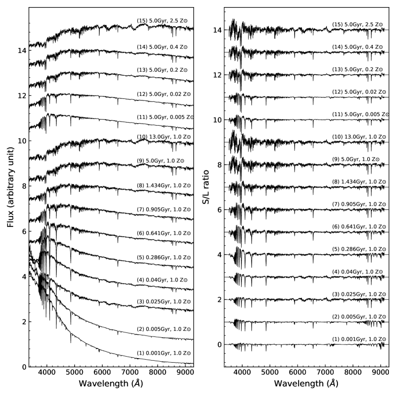
Figure 1: In the left panel, SSPs with different ages and metallicities are from BC03. The first 10 SSPs have different ages but the same metallicity (solar metallicity), and the last 5 SSPs have the same age (5 Gyr) but different metallicities. They are normalized at 5500Å and the $i^{th}$ SSP has been shifted upward $i-1$ unites. The right panel shows the ratios of small-scale to large-scale component of each SSPs and the $i^{th}$ is shifted upward $i-1$ unites.

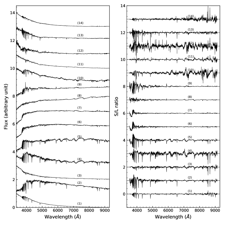
Figure 2: The left panel displays the 14 eign-spectra which are resulted from a Principal Component Analysis of the BC03 SSPs and used in this work as the model templates. The right panel displays the corresponding ratio spectra between the small scale and large scale components.

2.1 Spectral decomposition

In our analysis, we first decompose a spectrum into two components, one small-scale component, $S$, and one large-scale component, $L$. Roughly speaking, the $L$ component can be considered as the continuum shape of the spectrum, and the $S$ component as the composition of absorption and emission line features. We adopt a moving average method to separate small-scale and large-scale components. Specifically, the large-scale component is firstly obtained through

$$F_{L}^{\rm a}(\lambda)=\frac{1}{\Delta\lambda}\int_{\lambda-\Delta\lambda/2}^{\lambda+\Delta\lambda/2}F^{\rm a}(\lambda^{\prime})\,d\lambda^{\prime},$$ (3)

where $\Delta\lambda$ is the size of the wavelength window. The small-scale component is simply defined as

$$F_{S}^{\rm a}(\lambda)=F^{\rm a}(\lambda)-F_{L}^{\rm a}(\lambda).$$ (4)

Using equation (2), we can write

$$F_{L}^{\rm a}(\lambda) = \frac{1}{\Delta\lambda}\int_{\lambda-\Delta\lambda/2}^{\lambda+\Delta\lambda/2}F(\lambda^{\prime})\cdot{\cal A}(\lambda^{\prime})\,d\lambda^{\prime}$$ (5)

$$\approx \frac{{\cal A}(\lambda)}{\Delta\lambda}\int_{\lambda-\Delta\lambda/2}^{\lambda+\Delta\lambda/2}F(\lambda^{\prime})\,d\lambda^{\prime},$$

where an approximation is made in the second line that $\Delta\lambda$ is small and ${\cal A}(\lambda)$ is smooth so that ${\cal A}$ varies little over $\Delta\lambda$. It is then easy to see that

$$F_{L}^{\rm a}(\lambda)=F_{L}(\lambda)\cdot{\cal A}(\lambda),$$ (6)

where $F_{L}(\lambda)$ is the large-scale component of the intrinsic spectrum $F(\lambda)$. Similarly, equation (4) can be written as

$$F_{S}^{\rm a}(\lambda) = \left[F(\lambda)-F_{L}(\lambda)\right]\cdot{\cal A}(\lambda)$$ (7)

$$= F_{S}(\lambda)\cdot{\cal A}(\lambda),$$

where $F_{S}(\lambda)$ is the small-scale component of the intrinsic spectrum. From equations (6) and (7), we see that the ratio between the small-scale and large-scale components is dust free:

$$R^{\rm a}(\lambda)=\frac{F_{S}^{\rm a}(\lambda)}{F_{L}^{\rm a}(\lambda)}=\frac{F_{S}(\lambda)}{F_{L}(\lambda)}=R(\lambda),$$ (8)

where $R(\lambda)$ is the ratio of the intrinsic spectrum.

As mentioned, our method of measuring the relative dust attenuation curves was motivated from Wilkinson et al. (2015), which originally proposed the idea of decomposing an observed spectrum into small- and large-scale components before performing full spectral fitting. In that study, the decomposition was done by applying a high-pass filter (HPF) to the Fourier transform of the observed spectrum, thus removing large-scale features through the use of an empirically chosen window function. The filtered spectrum containing only small-scale features is then fitted to the model templates that are filtered in the same way, producing the best-fit, dust-free spectrum. This approach is not applicable to our method, however. First, we need to obtain both the small-scale and large-scale components simultaneously, as we want to determine the best-fit stellar spectrum by fitting the ratio between the small and large-scale components, $R_{\lambda}$, instead of the filtered spectrum (i.e. the small-scale component only) as in Wilkinson et al. (2015). Second, the effect of dust attenuation to the small-scale component is not zero, and it is the $S/L$ ratio that is not affected by the dust attenuation, as equation (8) shows. Using equations (5) and (7), one can see that a moving average filter is ideal to meet these conditions.

It must be realized that the above relations are derived under the assumption that all the stellar populations have the same attenuation given by ${\cal A}(\lambda)$. In reality, dust attenuation may be more complicated and, in particular, may be different for different stellar populations. Along this line, Charlot & Fall (2000) proposed a two-component dust model, in which old stars are assumed to be mixed uniformly with a diffuse dust distribution while young stars are assumed to be embedded in birth clouds of stars that have larger dust optical depth than the diffuse component. This model is motivated by the empirical relation between stellar and nebular dust attenuation (Calzetti et al., 2000).

More generally, suppose that the $j^{th}$ stellar population (not necessarily a SSP) has an attenuation curve of ${\cal A}^{j}(\lambda)$, defined by

$${\cal A}^{j}(\lambda)=e^{-\tau^{j}(\lambda)},$$ (9)

where $\tau^{j}(\lambda)$ is the dust optical depth at wavelength $\lambda$, which is different for different stellar populations. The ratio between the small-scale and large-scale components can then be written as

$$R^{\rm a}(\lambda)=\frac{\sum_{j}x_{j}F^{j}_{S}(\lambda)e^{-\tau^{j}(\lambda)}}{\sum_{j}x_{j}F^{j}_{L}(\lambda)e^{-\tau^{j}(\lambda)}}\,,$$ (10)

where $F^{j}_{S}$ and $F^{j}_{L}$ are the small-scale and large-scale spectrum of the $j^{th}$ population. This equation reduces to equation (8), as expected, if $\tau^{j}(\lambda)$ is the same for all ‘$j$’ (which is the case if the dust distribution is a screen in front of the galaxy, as assumed above), or the intrinsic spectra of different stellar populations are the same.

Consider another simple case in which $\tau^{j}(\lambda)\ll 1$. In this case, one can write

$$R^{\rm a}(\lambda) \approx\frac{\sum_{j}x_{j}F^{j}_{S}(\lambda)[1-\tau^{j}(\lambda)]}{\sum_{j}x_{j}F^{j}_{L}(\lambda)[1-\tau^{j}(\lambda)]}$$ (11)

$$=\frac{T_{S}(\lambda)\sum_{j}x_{j}F_{S}^{j}(\lambda)}{T_{L}(\lambda)\sum_{j}x_{j}F^{j}_{L}(\lambda)},$$

where

$$T_{S}(\lambda)=1-\left<\tau\right>_{S}(\lambda)=1-\frac{\sum_{j}x_{j}F^{j}_{S}(\lambda)\tau^{j}(\lambda)}{\sum_{j}x_{j}F^{j}_{S}(\lambda)}\,,$$ (12)

and

$$T_{L}(\lambda)=1-\left<\tau\right>_{L}(\lambda)=1-\frac{\sum_{j}x_{j}F^{j}_{L}(\lambda)\tau^{j}(\lambda)}{\sum_{j}x_{j}F^{j}_{L}(\lambda)}.$$ (13)

Note that both $\left<\tau\right>_{S}(\lambda)$ and $\left<\tau\right>_{L}(\lambda)$ are weighted averages of $\tau^{j}(\lambda)$. We have estimated $T_{S}(\lambda)/T_{L}(\lambda)$ using realistic spectra and attenuation curves, and found the ratio to depend only weakly on $\lambda$ for $\tau^{j}<1$, so that $R^{\rm a}(\lambda)$ is again independent of dust attenuation. However, for $\tau^{j}>1$, the ratio $R^{\rm a}(\lambda)$ can be affected significantly by the differences in dust attenuation among different stellar populations. We thus conclude that, $R^{\rm a}(\lambda)$ can well reflect the properties of the underlying intrinsic spectrum under certain assumptions. Throughout this paper we assume $R^{\rm a}(\lambda)\approx R(\lambda)$. Actually in previous studies, dust is commonly treated as a screen in front of the whole galaxy or a given region of the galaxy, so that all the stellar populations in the galaxy/region have the same attenuation. In reality this cannot be always true. We will come back and consider more general cases in the future.

2.2 The fitting procedure

In our modeling of galaxy spectra, we fit the ratio $R^{\rm a}(\lambda)$ obtained from an observed spectrum with the corresponding ratio of the model spectrum. To this end, we decompose each model template to obtain its small-scale and large-scale components as defined by equations (3) and (4). For a given set of fitting coefficients, $\{x_{j}\}$, we obtain the model prediction of the ratio,

$$R^{\rm m}(\lambda)=\frac{f_{0}\sum_{j=1}^{N_{*}}x_{j}f_{S}^{j}(\lambda)}{f_{0}\sum_{j=1}^{N_{*}}x_{j}f_{L}^{j}(\lambda)},$$ (14)

where $N_{*}$ is the number of templates, $f_{S}^{j}(\lambda)$ and $f_{L}^{j}(\lambda)$ are the small-scale and large-scale components of the $j^{th}$ template, $f^{j}(\lambda)$, respectively. In the equation, the constant $f_{0}$ is the normalization of the model template, and is the same for all the $f^{j}_{S}(\lambda)$ and $f^{j}_{L}(\lambda)$. The predicted ratio $R^{\rm m}(\lambda)$ is then compared with the observed ratio $R^{\rm a}(\lambda)$ to determine $\{x_{j}\}$. The fitting is carried out by using MPFIT, which is a non-linear Least-squares Fitting code in IDL (Markwardt, 2009). We should point out that, the fact that the normalization factor $f_{0}$ is cancelled out in equation (14) indicates that this factor cannot be directly determined from this fitting procedure. We will come back to this point later.

In principle, one can use all the SSPs from the BC03 library, or a random subset, as the model templates for the above fitting process. SSPs with different ages and metallicities have different small-scale features. Similarly, the small-scale to large-scale (S/L) component ratios of different SSPs also have different features. This is shown in Figure 1, where the first 10 SSPs have different ages but the same metallicity (solar metallicity), while the last 5 have the same age (5 Gyr) but different metallicities. The left-hand panel shows the original SSPs and the right-hand panel shows the corresponding S/L ratio spectra. It is obvious that different SSPs have different absorption line strengths and other broader features. It is these differences that allow us to derive constraints on the stellar populations from a galaxy spectrum.

In order to speed up the fitting process, we construct a small set of model templates by applying the technique of Principal Component Analysis (PCA, Deeming 1964) to the BC03 SSP spectra. PCA can effectively reduce the size of the template library, as the principal features of the library can be described by the first few eigen-spectra. For instance, Li et al. (2005) obtained galactic eigen-spectra using PCA and showed that the first nine eigen-spectra already provided the base to model the stellar spectra of the galaxies in Sloan Digital Sky Survey Data Release 1 (SDSS DR1, Abazajian et al. 2003). In our analysis, we apply the PCA to the 1326 BC03 SSPs, and we adopt the first 14 eigen-spectra resulted from the PCA as the model templates for our spectral fitting. The cumulative contribution to variance by the first 14 eigen-spectra is 99.985%, indicating that they contain nearly all the information of the original 1326 SSPs. Figure 2 displays the 14 eigen-spectra (the left panel), as well as the corresponding S/L ratio spectra (the right panel). We should point out that the number of eigen-spectra is determined so as to include as much as possible information of the original SSPs, and simultaneously to reduce as much as possible the computing time. We have repeated our tests to be presented below, by adopting a different number of eigen-spectra, and found that the spectral fitting is little affected as long as the majority of the original information of the whole SSP library ($>99\%$) is contained in the adopted eigen-spectra.

Once the coefficients, $x_{j}$, are obtained from the fitting, the best fitting spectrum, $F^{\rm fit}$, which is expected to not contain the effect of dust attenuation, can be reconstructed by

$$F^{\rm fit}(\lambda)=f_{0}\sum_{j=1}^{{N_{*}}}x_{j}f^{j}(\lambda).$$ (15)

Note that the normalization factor $f_{0}$ is unknown, and it is set to be arbitrary for the moment. This means that the fitting procedure described above gives only the shape of the dust-free spectrum. The shape of the dust attenuation curve can then be obtained by comparing the best fitting spectrum with the observed spectrum:

$${\cal A}(\lambda)=\frac{F^{\rm a}(\lambda)}{F^{\rm fit}(\lambda)}.$$ (16)

Conventionally, ${\cal A}(\lambda)$ is written as

$${\cal A}(\lambda)=10^{-0.4\cdot A(\lambda)},$$ (17)

where $A(\lambda)$ is the dust attenuation at the wavelength of $\lambda$. In practice, we normalize both $F^{\rm a}(\lambda)$ and $F^{\rm fit}(\lambda)$ at a given wavelength,

$$\lambda_{V}=5500\mbox{\AA},$$ (18)

and we have

$$A(\lambda)-A_{V}=2.5\log_{10}\frac{\tilde{F}^{\rm fit}(\lambda)}{\tilde{F}^{\rm a}(\lambda)},$$ (19)

where $A_{V}$ is the dust attenuation at $\lambda_{V}$, and

$$\tilde{F}^{\rm fit}(\lambda) =F^{\rm fit}(\lambda)/F^{\rm fit}(\lambda_{V}),$$

$$\tilde{F}^{\rm a}(\lambda) =F^{\rm a}(\lambda)/F^{\rm a}(\lambda_{V})$$ (20)

are the dust-free and the observed spectrum normalized at $\lambda_{V}$, respectively. Note that the factor $f_{0}$ is implicitly contained in both $F^{\rm fit}(\lambda)$ and $F^{\rm fit}(\lambda_{V})$, and so is cancelled out due to the normalization. Therefore, what we obtain from this fitting procedure is the relative dust attenuation curve, i.e. $A(\lambda)-A_{V}$, which is the dust attenuation as a function of wavelength relative to the attenuation at $\lambda_{V}$.

Equation (19) shows that our method provides a direct measurement of the relative dust attenuation curve, with no need to assume a functional form for the curve. In practice, however, it may still be desirable to use a parametric form to represent the curve. As shown below, our measurements of $A(\lambda)-A(V)$ can well be represented by a second-order polynomial in most (if not all) cases,

$$A(\lambda)-A_{V}=a_{1}\lambda^{-1}+a_{2}\lambda^{-2}.$$ (21)

The parameters $a_{1}$ and $a_{2}$ are to be obtained by fitting the above function to the $A(\lambda)-A_{V}$ measured by using equation (19).

Given the measured $A(\lambda)-A_{V}$ and setting $\lambda=\lambda_{B}=4400$Å, we therefore can get the $(B-V)$ color excess

$$E(B-V)=A_{B}-A_{V},$$ (22)

where $A_{B}$ is the dust attenuation at the wavelength, $\lambda_{B}$, corresponding to the $B$-band. Similarly, the selective attenuation curve, defined as $[A(\lambda)-A_{V}]/[A_{B}-A_{V}]$, can also be obtained. In practice, dust attenuation is sometimes described by the total attenuation curve, defined as

$$k(\lambda) =\frac{A(\lambda)}{E(B-V)}=\frac{A(\lambda)}{A_{B}-A_{V}}$$ (23)

$$=\frac{A(\lambda)-A_{V}}{A_{B}-A_{V}}+R_{V},$$

where $R_{V}$ is the value of the total attenuation curve in the $V$-band,

$$R_{V}=A_{V}/E(B-V).$$ (24)

$R_{V}$ is also known as the ratio of the total to selective attenuation in the $V$-band.

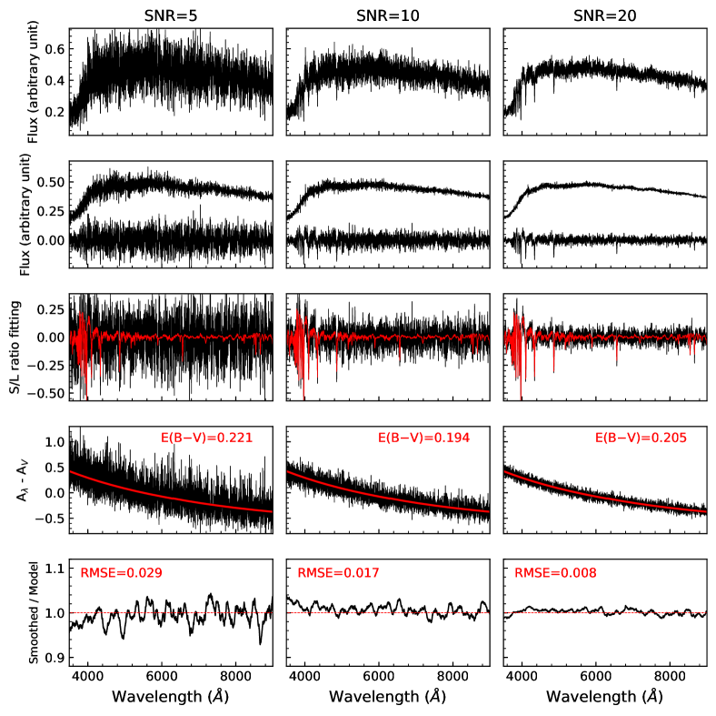
Figure 3: Examples of the fitting procedure for measuring relative dust attenuation curves and $E(B-V)$. Panels from left to right correspond to three mock spectra with different signal-to-noise ratios (SNRs): 5, 10 and 20. The mock spectra are constructed from a same intrinsic dust-free spectrum, and are reddened with a Calzetti attenuation curve assuming a color excess of $E(B-V)=0.2$. The top panels display the mock spectra, and panels in the second row show the small-scale and large-scale components of each spectrum. In the third row, the black line in each panel is the ratio of small-scale to large-scale component (S/L), while and the red line plots the S/L of the best-fitting model spectrum. In the fourth row, the black line is the recovered relative attenuation curve and the red line is the input attenuation curve. The $E(B-V)$ estimated from the measured attenuation curves is 0.221, 0.194, and 0.205 respectively, as indicated. In the bottom panels, the black lines show the ratios of the measured attenuation curve (smoothed for clarity) to the input one. The root square mean error (RMSE) of these curves is 2.9%, 1.7% and 0.8%, also indicated.

2.3 Examples

Figure 3 shows some examples to demonstrate the step-by-step application of our method to measure the relative dust attenuation curve, $A(\lambda)-A_{V}$, as well as the color excess, $E(B-V)$. The three panels in the first row display three mock spectra that correspond to $E(B-V)=0.2$ but have different Gaussian signal-to-noise ratios SNR=5, 10, and 20, as indicated on the top of the figure. Here a Calzetti dust curve (Calzetti et al., 2000) is adopted to create the mock spectra, and the procedure to construct the mock spectra will be detailed in the next section. In the second row, the moving average filter (see Eqn. 3 and 4) is applied to decompose each spectrum into the large-scale and small-scale components, which are plotted separately in each panel. The third row shows the small- to large-scale spectral ratio in black lines, and the best-fitting ratio (see Eqn. 14) in red lines, as obtained from the non-linear fitting described above. The coefficients obtained from the fitting are then used to derive the best-fitting model spectrum (see Eqn. 15), which is expected to be dust-free. The relative dust attenuation curves, given by the ratio between the original spectra and the best-fitting models (see Eqn. 19), are shown as the black lines in the fourth row. The input attenuation curve is repeated in the three panels as a red line for comparison. The $E(B-V)$ values obtained from our measured attenuation curves (see Eqn. 22) are 0.221, 0.194 and 0.205 for the three SNRs, respectively, as indicated in each panel, all very close to the input value, $E(B-V)=0.2$. In the bottom panels, we show the ratios of the measured attenuation curve to the input attenuation curve, which are smoothed for clarity. As one can see, our method recovers the input attenuation curve very well. The rms deviations of the measured attenuation curves around the input one are $2.9\%$, $1.7\%$ and $0.8\%$ for the three SNRs, respectively.

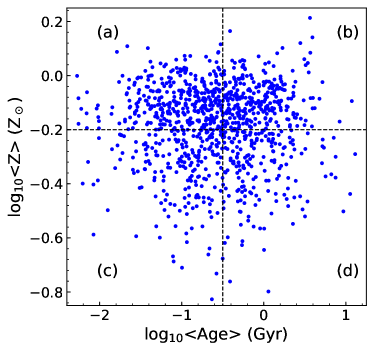
Figure 4: The distribution of mean age and mean metallicity of the mock spectra. We divide the age-metallicity space roughly into four regions, (a), (b), (c) and (d).

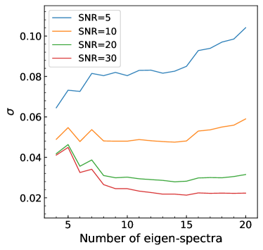
Figure 5: Tests on the effects of different number of eigen-spectra. Here the standard deviation ($\sigma$) of the difference between the output and input $E(B-V)$ values is plotted against the number of eigen-spectra. SNRs are indicated in this figure.

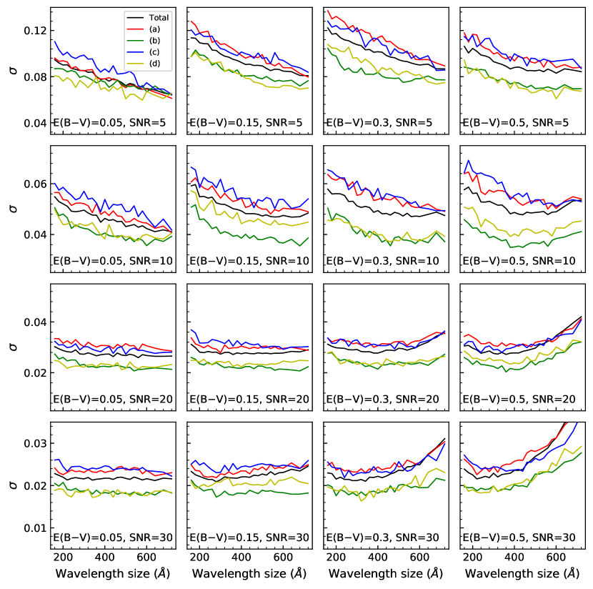
Figure 6: Tests on the effects of the wavelength window size used to define the small- and large-scale components of spectra. Here the standard deviation ($\sigma$) of the difference between the output and input $E(B-V)$ values is plotted against the wavelength window size. In each panel, the input value of $E(B-V)$ and the signal-to-noise ratio, SNR are indicated. The red, green, blue, yellow lines correspond to spectra in the (a), (b), (c), (d) regions, respectively. The black line is the result for all the spectra in the four regions.

3 Test with mock spectra

3.1 The mock spectra

In order to test the reliability of our method, we have created a series of synthetic spectra from the BC03 SSPs. We first pick 150 SSPs out of the 1326 BC03 SSPs, with 25 different ages and 6 different metallicities. For each metallicity, the 25 SSPs are chosen so as to cover the full range of age from 0.001 Gyr to 18 Gyr, with approximately equal intervals in the logarithm of the age. We then randomly select one of the 25 SSPs for every metallicity, and the six selected spectra of different metallicites and ages are then normalized at 5500Å and combined with random weights. We repeat this step 1000 times, thus creating 1000 synthetic mock spectra with a wide coverage of age and metallicity, as shown in Fig. 4. In the figure, the age-metallicity space is roughly divided into four regions as indicated by the vertical and horizontal lines: (a) young age and high metallicity, (b) old age and high metallicity, (c) young age and low metallicity, (d) old age and low metallicity. Each of the mock spectra is reddened with a Calzetti dust curve (Calzetti et al., 2000), but assuming four different color excesses: $E(B-V)=0.05$, $0.15$, $0.3$, and $0.5$. Finally, a Gaussian noise with SNR=5, 10, 20, or 30 is added to each spectrum. This procedure results in a total of 16,000 mock spectra, which are used to test our method.

We would like to point out that some of the mock spectra may not be physically meaningful, e.g. those with extremely old ages but high metallicities and those with young ages but low metallicities. We do not exclude these spectra from our test, because the inclusion of them does not affect our test results, as we will show below.

3.2 The choice of eigen-spectra number

As mentioned, we adopt the first 14 eigen-spectra resulted from the PCA analysis as the model templates for our spectral fitting. With the mock spectra generated above, we have examined the potential effect of using different numbers of eigen-spectra on the measurement of $E(B-V)$. For a given number of eigen-spectra and the mock spectra with a given SNR, we calculate the standard deviation, $\sigma$, of the difference between the output and input $E(B-V)$ values, and we use this quantity to indicate the goodness of our method in recovering the true $E(B-V)$. The result of this analysis is shown in Fig. 5, which plots $\sigma$ as function of the number of eigen-spectra for four different SNRs.

The figure shows that, for mock spectra with SNR$>10$, the value of $\sigma$ decreases as one adopts more and more eigen-spectra in the fitting, but $\sigma$ does not decrease any more when the number of eigen-spectra exceeds $\sim 15$. The value of $\sigma$ keeps roughly constant for SNR=10 and even increases for SNR=5. In spectra with low SNRs, features on small scales such as stellar absorption lines can be well dominated by noise, and so the use of too many eigen-spectra actually leads to poor fits. Overall, the figure indicates that the use of $8$-$15$ eigen-spectra appears to be able to achieve a compromise among different SNRs. We opt for the first 14 eigen-spectra considering mainly the fact that the $\sigma$ starts to increase with 15 eigen-spectra at all SNRs. Nevertheless, we note that the variation of $\sigma$ with the number of eigen-spectra used is in general modest in comparison to that produced by different SNRs.

3.3 The choice of filtering window size

As mentioned before, filtering to separate a spectrum into small- and large-scale components plays an important role in our method, and it is critical to find a suitable choice of the wavelength window size for the filtering. For this purpose, we have adopted window sizes ranging from 160Å to 720Å when filtering the mock spectra. Fig. 6 shows $\sigma$ versus the wavelength window size, for mock spectra of different $E(B-V)$ and SNRs. Defined in the same way as above, the $\sigma$ is an indicator of the goodness of our method. The four colorful curves in each panel correspond to the four regions divided in Fig. 4, while the black curve is for all the spectra with the given $E(B-V)$ and SNR. Generally, as expected, the value of $\sigma$ decreases as SNR increases. In addition, for low values of SNR (5 and 10), $\sigma$ tends to decrease as the wavelength window size increases, but the trend reverses when SNR and $E(B-V)$ are high.

The results shown in Fig. 6 suggest that the wavelength window size should be chosen to be about 500Å for SNR smaller than 10 and about 300Å for higher SNR. This dependence of smoothing window size on SNR is understandable. A larger window size can reduce the effects of noise in the low SNR spectra more effectively, while a smaller window size is needed to retain more real features in the spectra with high SNR. Spectra with older stellar ages (green and yellow lines) also trend to have lower $\sigma$ than younger ones (red and blue lines), indicating that our method works better for older stellar populations. However, the differences in the results among the four different regions are not large in comparison with the effects of the SNR and the wavelength window size.

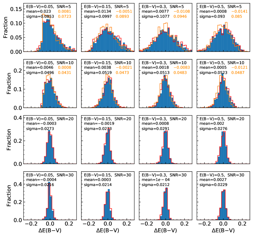
Figure 7: Tests with mock spectra that have different $E(B-V)$ values and signal-to-noise ratios (SNR). Here the distribution is shown with respect to $\Delta E(B-V)$), the difference between the fitting result of $E(B-V)$ and the input value. The input $E(B-V)$ and SNR are indicated in each panel. The mean value and standard deviation of $\Delta E(B-V)$ are indicated by ‘mean’ and ‘sigma’, respectively. For all cases, we choose a wavelength window size of 300Å. The red histograms show the results of ‘unreasonable’ spectra that locate in upper-right and lower-left corners of Fig. 4. For lower-SNR spectra with SNR=5 and 10, we also show the test for a window size of 500Å, plotted as the orange histograms in the top two rows.

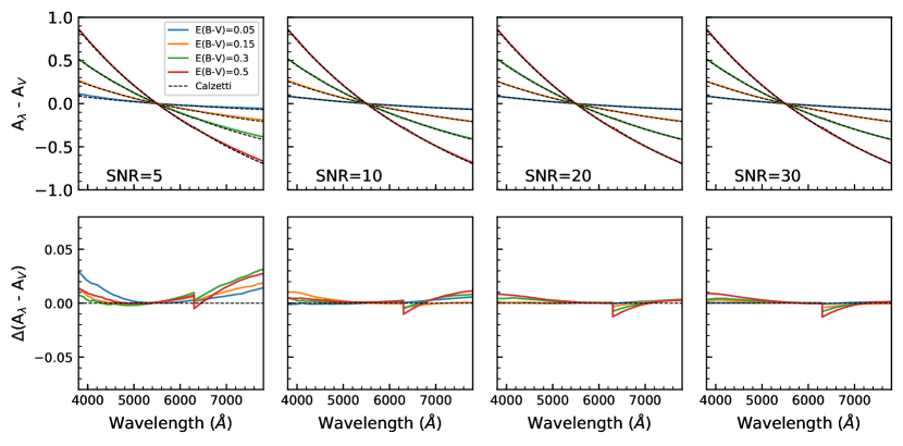
Figure 8: The first row shows the medians of all relative dust attenuation curves in each $E(B-V)$ and SNR bins. The second row shows the differences between the median curves and the Calzetti curve.

3.4 Test results

Fig. 7 shows the results of our test on mock spectra. Each panel is based on 1000 spectra with given $E(B-V)$ and SNR, as described in §3.1. The filled histogram in each panel shows the fraction of the 1000 fitting as a function of the difference between the output and input values of $E(B-V)$, referred to as $\Delta E(B-V)$ in what follows. In each panel, the input values of $E(B-V)$ and SNR, the mean and standard deviation ($\sigma$) of $\Delta E(B-V)$, are indicated. We have chosen a wavelength window size of 300Å for all the cases, according to the analysis presented in the previous subsection. For low-SNR spectra with SNR=5 and 10, we repeat the test using a larger window size of 500Å, and plot the results as the orange histograms in the top two rows. As can be seen, the results change little with varying wavelength window sizes.

The standard deviation, $\sigma$, decreases as SNR increases, but its dependence on the input $E(B-V)$ is quite weak. The distribution of $\Delta E(B-V)$ in most cases is roughly a Gaussian centered at $\Delta E(B-V)\sim 0$, indicating that the model inference is unbiased. The only exception is the case shown in the first panel, where the distribution is skewed to positive values of $\Delta E(B-V)$. In this case, the inputs of $E(B-V)$ and SNR are both small. We note that increasing the wavelength window size for the moving average filter does not make a significant improvement of the $E(B-V)$ measurement in such low-SNR and low-$E(B-V)$ cases.

We also show the results for “unreasonable” mock spectra as the red histograms in individual panels. These spectra are located in regions $b$ and $c$ in Fig. 4: they either have old ages and high metallicities, or young ages and low metallicities. The distributions of $\Delta E(B-V)$ for these spectra are almost the same as those of the full samples at given $E(B-V)$ and SNR, indicating that the inclusion of such spectra does not introduce biases into our test results.

As described in §2.2, our method can recover the relative attenuation curve. As a demonstration, the upper row of Fig. 8 shows the median $A_{\lambda}-A_{V}$ curve at given $E(B-V)$ and SNR. Panels from left to right are for different SNR bins, and the different colors in each panel are for different $E(B-V)$ bins. For each case the corresponding Calzetti curve is plotted as a dotted line. The differences between the median curves output from our method and the input Calzetti curve are shown in the lower row. As one can see, our method indeed recovers the input curve very well in all cases and at all wavelengths. The largest difference is $\sim 0.03$ magnitude, and this occurs at lowest SNR (SNR=5) and at both short ($<5000$Å) and long wavelengths ($>6500$Å). At higher SNRs the difference is generally very small, less than 0.01 magnitude at all wavelengths. There is a slight but noticeable jump at $\sim 6200$Å in all cases. This is caused by the fact that the Calzetti curve is a piecewise function with two sub-functions separated at a fixed wavelength, while the attenuation curves output from our method are smooth, thus not necessarily following any predefined functional forms.

To conclude, the results of the test demonstrate that the input $E(B-V)$ are well recovered by our method for various cases. The systematic bias in $\Delta E(B-V)$ is quite small, indicating that potential uncertainties, such as that produced by the dust-age degeneracy, is well taken care of by our method.

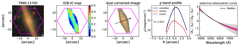
Figure 9:

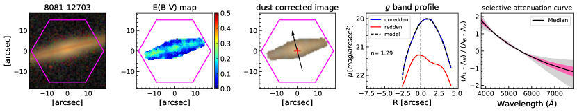
Figure 10:

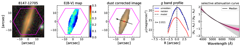
Figure 11:

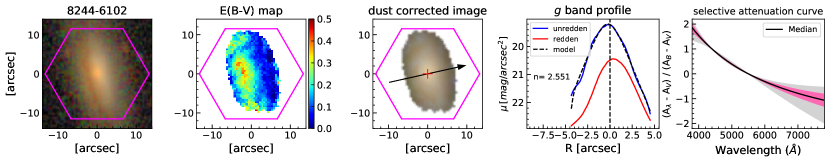
Figure 12:

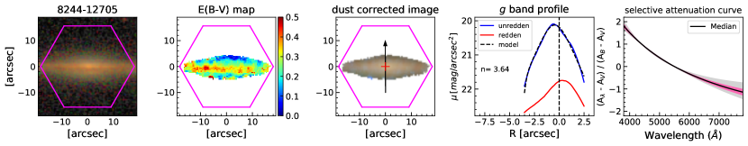
Figure 13:

Figure 14: There are five panels in each row. The first one is SDSS $gri$ color-composite image with the MaNGA footprint in magenta. The second one is the $E(B-V)$ map derived from our method. The third one is dust corrected $gri$ color-composite image. The red cross shows the center of the integral field. In the fourth panel, the red line is reddened brightness profile while the blue line is un-reddened brightness profile along the direction of arrow in the third panel. The un-reddened brightness profile is fitted by a model that the black dash line shows. $n$ is the key parameter of this model. The last panel shows the selective attenuation curves measured from our method. The black solid line is the median, the pink region shows the standard deviation of the spaxels around the median, and the grey region covers the range spanned by all the individual spaxels.

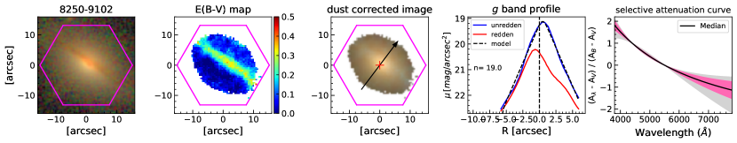
Figure 14:

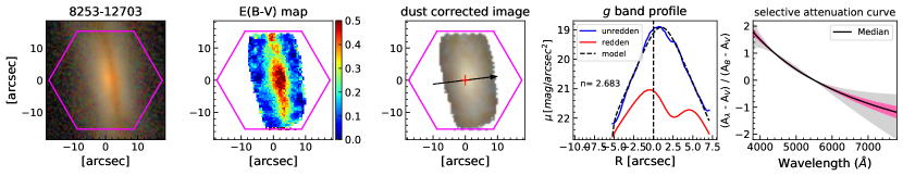
Figure 15:

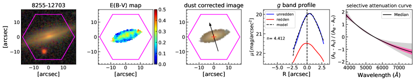
Figure 16:

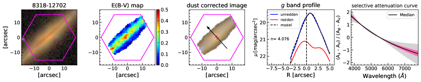
Figure 17:

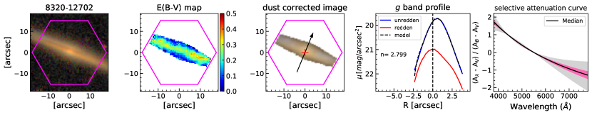
Figure 18:

Figure 19: (Continued). There are five panels in each row. The first one is SDSS $gri$ color-composite image with the MaNGA footprint in magenta. The second one is the $E(B-V)$ map derived from our method. The third one is dust corrected $gri$ color-composite image. The red cross shows the center of the integral field. In the fourth panel, the red line is reddened brightness profile while the blue line is un-reddened brightness profile along the direction of arrow in the third panel. The un-reddened brightness profile is fitted by a model that the black dash line shows. $n$ is the key parameter of this model. The last panel shows the selective attenuation curves measured from our method. The black solid line is the median, the pink region shows the standard deviation of the spaxels around the median, and the grey region covers the range spanned by all the individual spaxels.

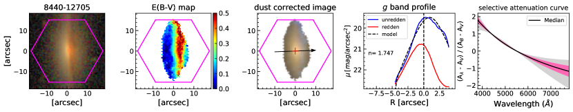
Figure 19:

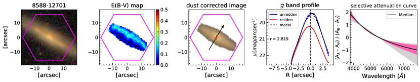
Figure 20:

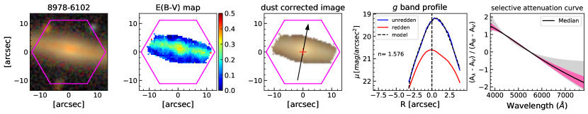
Figure 21:

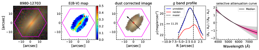
Figure 22:

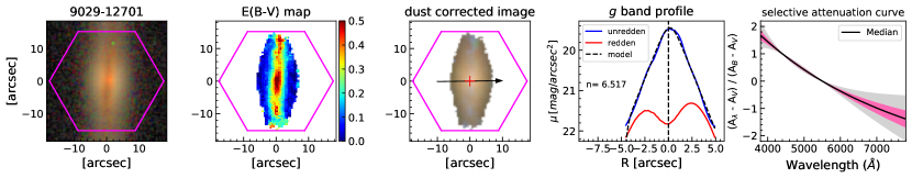
Figure 23:

Figure 24: (Continued). There are five panels in each row. The first one is SDSS $gri$ color-composite image with the MaNGA footprint in magenta. The second one is the $E(B-V)$ map derived from our method. The third one is dust corrected $gri$ color-composite image. The red cross shows the center of the integral field. In the fourth panel, the red line is reddened brightness profile while the blue line is un-reddened brightness profile along the direction of arrow in the third panel. The un-reddened brightness profile is fitted by a model that the black dash line shows. $n$ is the key parameter of this model. The last panel shows the selective attenuation curves measured from our method. The black solid line is the median, the pink region shows the standard deviation of the spaxels around the median, and the grey region covers the range spanned by all the individual spaxels.

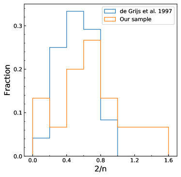
Figure 25:

Figure 26: The distribution of parameter $2/n$, which is a parameter in Equation 26 controlling the central sharpness of a vertical surface brightness profile. The blue histogram is the result from our sample, while the orange histogram is obtained from de Grijs et al. (1997).

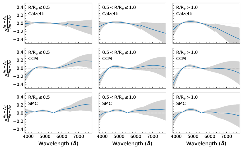
Figure 27:

Figure 28: The differences of the fitted Calzetti (upper panels), CCM (middle panels) and SMC (bottom panels) model curves relative to the measured selective attenuation curve of the 15 MaNGA galaxies. Panels from left to right are the results for spaxels at three different radial intervals as indicated. In each panel, the solid blue line is the median of all the spaxels at the given radii, and the grey region indicates the standard deviation of the spaxels.

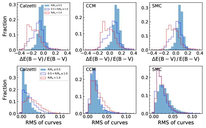
Figure 29:

Figure 30: Upper: Distribution of the relative difference of $E(B-V)$ between the fitted model curves of Calzetti, CCM and SMC (panels from left to right) and the measured curve. Plotted in different colors are results for spaxles at different radii, as indicated. Lower: Distribution of the rms scatter of the fitted curves around the measured one.

4 Applications to MaNGA galaxies

4.1 The MaNGA data

Mapping Nearby Galaxies at Apache Point Observatory (MaNGA) survey (Bundy et al., 2015; Yan et al., 2016a, b; Law et al., 2016; Wake et al., 2017) is one of the three core programs of SDSS-IV (Sloan Digital Sky Survey IV, Blanton et al., 2017). MaNGA aims to obtain spatially resolved spectroscopy of about 10,000 nearby galaxies. In the outskirts of galaxies, MaNGA can reach a SNR of 4–8 (per Å per $2\arcsec$ fiber) at 23 AB mag arcsec^-2 in the $r$-band. The wavelength coverage is between 3,600 and 10,300Å  with a spectral resolution $R\sim 2000$ (Drory et al., 2015). In this paper, we select galaxy samples from the Sloan Digital Sky Survey Data Release 14 (SDSS DR14, Abolfathi et al., 2018), which includes integral field spectroscopy (IFS) data from MaNGA for 2812 galaxies, including ancillary targets and $\sim 50$ repeated observations. We visually inspect the SDSS $gri$ color-composite images of all the galaxies in this release, and select 15 edge-on galaxies that have obvious dust lane features. Galaxies of this kind are much more affected by dust attenuation than those viewed from face-on, and thus provide more demanding tests of our method. In the rest of this paper, we will apply our method to the 15 galaxies to demonstrate that our method can effectively measure the spatially-resolved $E(B-V)$ maps and relative dust attenuation curves, even for these difficult cases.

4.2 Dust attenuation maps and profiles

In the current version of our code, velocity dispersion of the observed spectrum needs to be specified so that model templates can be adapted to the observed spectral resolution. We first use PPXF (Cappellari & Emsellem, 2004; Cappellari, 2017) to measure stellar kinematics and correct the broadening effect of velocity dispersion. We then apply our method to all the spatial pixels in the MaNGA datacubes whose continuum SNRs are greater than 5. Fig. 14 displays the two-dimensional maps obtained from our method for the 15 galaxies in our sample. The first panel in each row shows the SDSS $gri$ color-composite image of the galaxy in question, and the second panel is the $E(B-V)$ map obtained from our method. As one can see, the dust lanes in the original images are well reproduced in the $E(B-V)$ maps, in terms of both the spatial distribution and the relative strength.

Once the $E(B-V)$ map is obtained for a galaxy, we can correct the effect of dust attenuation on the $gri$ image. Since the FWHM (full width at half maximum) of the point-spread function (PSF) for MaNGA is $\sim 2.5\arcsec$, while that of the SDSS $gri$ image is $\sim 1.4\arcsec$, we convolve the SDSS image in $g$, $r$ and $i$ bands with a Gaussian kernel to match the MaNGA PSF, before correcting the dust attenuation in the images. As what we measure are relative, not absolute attenuation curves, we assume a Calzetti attenuation curve to estimate the absolute attenuation in $g$, $r$ and $i$ bands according to the estimated $E(B-V)$ map. The images in the three bands are then corrected for the dust attenuation, and combined to form a new $gri$ color-composite image, which is expected to be dust free. This corrected image is shown in the third panel for each galaxy. The dust lanes in the original images are no longer seen in the dust-corrected images. This can be seen more clearly in the fourth panel of each row, where the red and blue curves show, respectively, the original and corrected brightness profiles in the $g$-band, as measured along the arrow indicated in the third panel. Compared to the corrected brightness profile, the original one is not only lower in amplitude, but also asymmetric in shape due to the strong attenuation in dust lane regions. In almost all cases, the prominent features in the vertical surface brightness profiles produced by the dust absorption are no longer present in the dust-corrected profiles. The corrected profiles are roughly symmetric with respect to the peak, as is expected for axis-symmetric thin disks.

We attempt to fit the dust corrected brightness profiles with a vertical brightness profile model. Since galaxy disks are not infinitesimally thin, the three-dimensional luminosity density of the disk is typically written as

$$\nu(R,z)=\nu_{0}\exp(-R/R_{d})f(z).$$ (25)

The first part of this equation describes the surface brightness as a function of the radius $R$, which is assumed to have an exponential profile, with $R_{d}$ being the scale-length of the disk. The function $f(z)$ describes the surface brightness distribution in the vertical ($z$) direction (see §2.3.3 of Mo et al. (2010) for a review). A commonly adopted fitting function of $f(z)$ is

$$f_{n}(z)={\rm sech}^{2/n}\left(\frac{n|z|}{2z_{d}}\right),$$ (26)

where $n$ is a parameter controlling the shape of profile near $z=0$, and $z_{d}$ is the scale-height of the disk. In particular, $n=1$ corresponds to a self-gravitating isothermal sheet while $n=\infty$ corresponds to an exponential profile. Note that $f_{n}(z)$ decreases exponentially at large $|z|$, but a larger value of $n$ gives a steeper profile near the mid-plane. When fitting the observed profile, the effect of seeing on the observed data must be included. This is done by convolving the model profile with a Gaussian kernel that matches the MaNGA PSF. The best-fit model profile is plotted for each galaxy as the black dash line in the fourth panel of Fig. 14. For reference, we also indicate the values of $n$ in the corresponding panels. It is clear that the corrected profiles are well described by the model.

Fig. 26 shows the distribution of $2/n$ for the 15 galaxies in comparison with that obtained by de Grijs et al. (1997) from fitting the $K$-band images of 24 nearly edge-on spiral galaxies. The two distributions are qualitatively consistent with each other, suggesting again that our method is able to correct dust attenuation for nearly edge-on galaxies. Unfortunately, no quantitative comparison can be made, as the two samples are small and have different selections.

4.3 Dust attenuation curves

As described in §2.2, one important advantage of our method is that the relative dust attenuation as a function of wavelength (i.e. the relative attenuation curve) can be directly obtained without the assumption of a functional form for the shape of the attenuation curve or the adoption of a theoretical dust model. The selective attenuation curves measured from our method are plotted in the rightmost panel of each row in Fig. 14. The grey region covers the range spanned by all the individual spaxels in a given galaxy. The black solid line is the median, while the pink region shows the standard deviation of the spaxels around the median. The variance represented by the grey and pink regions shows that different spaxels may have different shapes of attenuation curves, suggesting that dust attenuation may not be described completely by a universal curve. Note that, by definition, the selective attenuation curves have a fixed value of unity at $\lambda_{B}$ (4400Å) and zero at $\lambda_{V}$ (5500Å), and this is why the variation among individual spaxels appears only at wavelengths shorter than $\sim 4000$Å and longer than $\sim 6000$Å.

In order to better understand the variation of the attenuation curve, we further examine the measured selective attenuation curves at different radii from the galactic center. We also compare the measured curves with the commonly-adopted dust curves in the literature. Here we consider three dust curves: the Calzetti attenuation curve for local starburst galaxies (Calzetti et al., 2000), the Milky Way extinction curve (Cardelli et al., 1989, CCM), and the Small Magellanic Cloud extinction curve (Gordon et al., 2003, SMC). We fit each of the measured attenuation curve with the three dust curves. Fig. 28 shows the differences of the fitted selective attenuation curve with respect to the measured curve, for spaxels in the following three radial intervals: $R/R_{e}\leq 0.5$, $0.5<R/R_{e}\leq 1$ and $R/R_{e}>1$. In each radial interval, we plot both the median (the solid blue line) and the standard deviation of the difference (the grey region), as a function of wavelength.

Overall, all the three curves deviate from the measurements to some degrees, but in different ways. At $R\leq 0.5R_{e}$, the Calzetti curve provides a best fit to the measurements, as shown in the top-left panel, while both CCM and SMC curves significantly deviate from the measurements. At $R>0.5R_{e}$, the CCM and SMC curves work better than the Calzetti one, and the SMC appears to behave slightly better than the CCM. As pointed out above, the selective attenuation curves have fixed values at $\lambda_{B}$ and $\lambda_{V}$. Thus, the wavelength-dependence shown in the figure may change if color excess in other two bands is used to normalize the curves.

In Fig. 30 we further examine the deviation of the three curves relative to our measurements by plotting the histograms of the relative difference of $E(B-V)$ (upper panels) and the rms deviation of the curves (lower panels). Consistent with results shown in the previous figure, the Calzetti curve shows the smallest deviation at $R\leq 0.5R_{e}$, with the distribution of $\Delta E(B-V)/E(B-V)$ centered at around zero and a rms less than 5%. At $R>R_{e}$, the CCM and SMC curves are better than the Calzetti curve, with smaller $\Delta E(B-V)/E(B-V)$ on average, while the three curves show similar rms in deviation. These results suggest that none of the three curves can universally describe the measured curves at all radii. The inner region of galaxies seems to prefer a Calzetti-like curve while the outer region prefers a SMC or Milky Way-like curve.

5 summary and discussion

We have developed a method to estimate the relative dust attenuation curve, $A(\lambda)-A_{V}$ (see equation 19), which is the dust attenuation as a function of wavelength relative to that at the fixed wavelength $\lambda_{V}$. For an observed spectrum of a galaxy or a specific region within a galaxy, our method first decomposes the spectrum into a small-scale component, $S$, and a large-scale component, $L$, by adopting a moving box average method. Assuming all the stellar populations that contribute to the observed spectrum have the same attenuation given by ${\cal A}(\lambda)$, we are able to show that the ratio of the two components, $R(\lambda)={F_{S}(\lambda)}/{F_{L}(\lambda)}$ (see equation 8), is free of dust attenuation. The observed $R(\lambda)$ can be modeled with a given theoretical library of simple stellar populations (SSPs), without the need for modeling the effect of dust attenuation in the fitting. The dust-free intrinsic spectrum is then reconstructed from the SSPs according to the corresponding coefficients that form the best-fit to $R(\lambda)$. Finally, the relative dust attenuation curve is obtained by comparing the observed spectrum with the ‘dust free’ model spectrum.

We have performed extensive tests of our method on a set of mock spectra covering wide ranges in stellar age and metallicity, as well as $E(B-V)$ and spectral signal-to-noise ratios (SNRs). These tests show that both the $E(B-V)$ and the relative dust attenuation curve can be well recovered as long as $E(B-V)>0.05$ and $SNR>5$. At lower $E(B-V)$ and smaller SNRs, on average, our method tends to overestimate $E(B-V)$ by $\lesssim 0.03$ magnitude (see Fig. 7). We have also tested our method on more realistic mock spectra using continuous star formation histories and including emission lines, finding no significant change in our results (see Appendix A and Fig. 32).

We have applied our method to the integral field spectroscopy (IFS) of 15 edge-on galaxies from the ongoing MaNGA survey, obtaining both the two-dimensional map and radial profile of $E(B-V)$ for each galaxy, as well as the spatially-resolved relative dust attenuation curve. Using the $E(B-V)$ maps we have corrected the effect of dust attenuation on the SDSS $gri$ image of these galaxies. The dust lanes in the original images become invisible in the images reconstructed from the attenuation-corrected spectra, and the vertical brightness profiles in a given band become almost symmetric and can be well described by a simple model proposed for the disk vertical structure.

We have compared the estimated dust attenuation curves of the 15 MaNGA galaxies with three commonly-used empirical models: the Calzetti attenuation curve for local starburst galaxies from Calzetti et al. (2000), the CCM extinction curve for Milky Way from Cardelli et al. (1989), and the SMC extinction curve for the Small Magellanic Cloud from Gordon et al. (2003). Although small in number, the MaNGA galaxies in our sample already show variations in the slope of dust attenuation curves (see the rightmost panels in Fig. 14), implying that the attenuation curves are not universally described by a single curve. Figs. 28 and 30 show that the Calzetti curve describe well the attenuation in the inner region ($R\leq 0.5R_{e}$) of the MaNGA galaxies, while a SMC or Milky Way-like curve works better for the outer region. This result may be attributed to the negative gradient of star formation rate observed in spiral galaxies. In this case, the inner region has stronger star formation than the other region, and is better described by a Calzetti curve which was initially proposed for local starburst galaxies.

Once the radial dependence is taken into account, i.e. by adopting a Calzeti curve for inner regions and a SMC or Milky Way curve for outer regions, the deviations in $E(B-V)$ of the model curves from the measured ones are relatively small, with a median of $\sim 10\%$ and a rms less than $\sim 10\%$ (see Fig. 30). This result is probably not unexpected given both the similarity of the different attenuation models and the relatively weak wavelength-dependence of the attenuation in the optical band. It is known that the various attenuation models differ more significantly in the ultraviolet. In particular, the CCM model presents a bump at around 2175Å, which is absent in the Calzetti and SMC curves. Therefore, previous observational studies of dust attenuation curves have mainly relied on broad-band spectral energy distribution (SED) including UV bands (e.g., Salmon et al., 2016; Battisti et al., 2017a, b; Salim et al., 2018; Tress et al., 2018; Decleir et al., 2019; Salim & Boquien, 2019). In many cases, these studies have also found evidence in support of variations in the slope of attenuation curves and/or the strength of the UV bump. In a recent theoretical paper (Narayanan et al., 2018), a model for the origin of such variations was developed, in which the variation in the attenuation curve slope depends primarily on complexities in the star-dust geometry, while the bump strength is primarily influenced by the fraction of unobscured O and B stars. In principle, if applied to galactic spectra covering the UV band, our method should be able to provide an independent way of quantifying the variations in the attenuation curve and the UV bump. Next-generation large spectroscopic surveys such as the Prime Focus Spectrograph surveys (PFS; Takada et al., 2014) will obtain high-quality spectra for hundreds of thousands of galaxies at $1\lesssim z\lesssim 2$, for which the rest-frame UV bump will be well covered in the observed spectrum. We expect to apply our method to those galaxies, thus directly deriving the selective dust attenuation curves for high-$z$ galaxies.

One important advantage of our method is that the estimated dust attenuation curve is independent of the shape of theoretical dust attenuation curves. In other words, this method provides a way to break the known degeneracy of dust attenuation with other properties of the stellar population in a galaxy, particularly stellar age and metallicity. Therefore, we can expect to have better constraints on the stellar age and metallicity by performing full spectral fitting to the ‘dust-free’ spectrum obtained using our method. In Appendix B we present a test of this hypothesis on a set of mock spectra, using a Bayesian approach to explore the potential degeneracy of model parameters. As can be seen there, the uncertainties in both the age and metallicity are indeed reduced significantly by using the estimated dust attenuation curve before the spectral fitting. We will come back to this point and further explore the potential of our method in improving stellar population synthesis techniques.

As emphasized, one limitation of our method is that the estimated dust attenuation curves are relative, but not absolute. Equation 24 indicates that, if one were to obtain the total (absolute) dust attenuation at given $\lambda$, it is necessary to know the value of $R_{V}$ (or, more generally, the total attenuation at any given wavelength that falls in the wavelength range covered). For instance, the $R_{V}$ of the Calzetti dust curve is 4.05, with a dispersion of 0.8 (Calzetti et al., 2000). In reality, however, $R_{V}$ may vary from galaxy to galaxy, and from region to region within a galaxy. Different galaxies or regions may have the same shape of attenuation curve, but different absolute attenuation values at a given wavelength due to the variation of $R_{V}$ (e.g., Reddy et al., 2015; Salim et al., 2018). One plausible way to determine $R_{V}$, thus the absolute attenuation curve, is to include data in near-infrared (NIR), e.g. photometry in $J$, $H$ and $K_{s}$ bands from existing NIR imaging surveys, where dust attenuation becomes negligible. For a given $R_{V}$, in practice, one may predict the apparent magnitudes in the NIR from the dust-free spectrum, $F^{\mbox{fit}}(\lambda)$, as obtained from fitting the $S/L$ ratio of the observed spectrum (see Eqn. 15). The value of $R_{V}$ and the absolute attenuation curve can then be derived by comparing the predicted NIR magnitudes with the observed ones. We will test and apply this idea in the future.

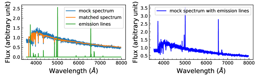
Figure 31: An example of mock spectrum with emission lines. In the left panel, light blue line is the mock spectrum without emission lines. Orange line is the best-fit stellar spectrum of the matched spectrum in the MaNGA sample (SDSS/DR14). Green line shows the observed emission lines in the matched MaNGA spectrum. The right-hand panel shows the final mock spectrum with emission lines, which is actually the sum of the blue and green lines in the left panel.

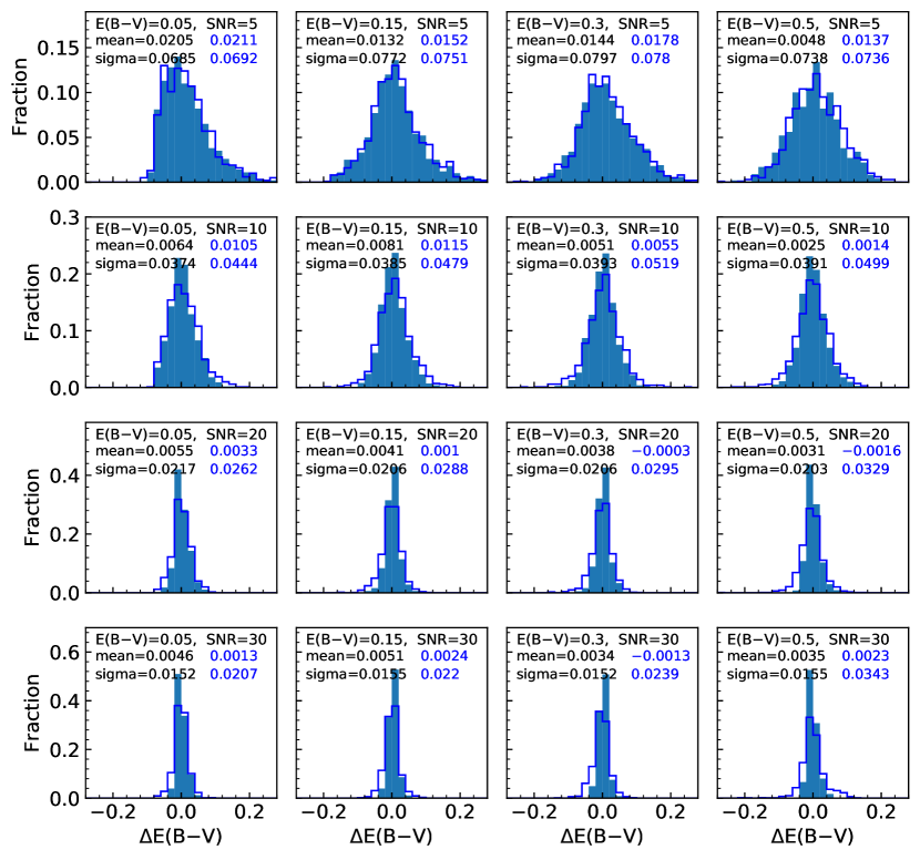
Figure 32: Tests on mock spectra generated with continuous SFH, with (unfilled histograms) or without (filled histograms) including emission lines. Panels from left to right correspond to different $E(B-V)$, and panels from top to bottom correspond to different signal-to-noise ratios (SNRs), as indicated. In each panel, the histograms show the distribution of the difference between the output and input value of $E(B-V)$, referred to as $\Delta E(B-V)$. Indicated in each panel are the mean value and standard deviation of $\Delta E(B-V)$ for both the filled (black) and unfilled (blue) histograms.

Appendix A Tests with more realistic mock spectra

In §3 we have tested our method of estimating dust attenuation curves on a set of mock spectra generated by linearly combining discrete simple stellar populations (SSPs) covering a wide range of stellar age and metallicity. In a real galaxy, however, stars are expected to form over an extended period of time with a continuous star formation history (SFH). In addition, observed spectra of galaxies often present emission lines produced by ionized gas. Here we present additional analyses by testing our method on a set of more realistic mock spectra with both continuous SFHs and emission lines. As we will show below, even with these additional complications, our method is still capable of recovering the input dust attenuation curves reliably and accurately.

A.1 Generating the mock spectra

For the SFH, we adopt the widely-used $\tau$-model in which the star formation rate declines with time exponentially,

$$\Psi(t)=\frac{1}{\tau}\frac{e^{-(t-t_{i})/\tau}}{1-e^{-(t_{0}-t_{i})/\tau}},$$ (A1)

where $\tau$ is the $e$-folding timescale, $t_{i}$ and $t_{0}$ are the starting time and the present time, respectively, so that $(t_{0}-t_{i})$ is the total duration of the SFH. A small $\tau$ and a large $(t_{0}-t_{i})$ thus correspond to a short duration of star formation at early times, which may be suitable for a galaxy dominated by old stellar populations. In contrast, a long $e$-folding timescale and a small value of $(t_{0}-t_{i})$ are suitable for young galaxies with steadily declining star formation. For simplicity, we adopt $t_{0}=14$ Gyr, and generate 1000 SFHs by randomly selecting $\tau$ and $t_{i}$ over the ranges of $0.01<\tau<100$Gyr and $0<t_{i}<13.9$Gyr, respectively. For a given SFH, we first convolve it with simple stellar populations (SSPs) given by the BC03 library (Bruzual & Charlot 2003), which are obtained using the Padova 1994 evolutionary tracks and a Chabrier initial mass function (Chabrier, 2003). This gives a noise-free composite spectrum, which is then reddened with a Calzetti attenuation curve, assuming four different color excesses: $E(B-V)$=0.05, 0.15, 0.3 and 0.5. Different levels of Gaussian noise are added to the spectrum to mimic signal-to-noise ratios of SNR=5, 10, 20 and 30, respectively. In total we have a set of 16,000 spectra that cover wide ranges of age, metallicity, SNR and color excess.

Finally, we add emission lines to each of the mock spectra. To do this, we take the real spectra of MaNGA galaxies in the SDSS/DR14, and perform full spectral fitting to each spectrum using the public pipeline pPXF (Cappellari & Emsellem, 2004; Cappellari, 2017). For each of our mock spectra, we find a counterpart spectrum from the real spectra of MaNGA, requiring that their SNRs are similar ($\Delta SNR<5$) and that the fitted spectrum and the mock spectrum are matched with each other most closely according to $\chi^{2}$ minimum. The starlight-subtracted emission lines of the counterpart spectrum are then added to the mock spectrum. Fig 31 displays an example of the mock spectra with emission lines. We have visually examined a considerable fraction of the mock spectra. In general, mock spectra with younger ages present stronger emission lines, while spectra of older ages present weaker emission lines, consistent with expectations.

A.2 Test results

We test our method on the mock spectra both before and after the emission lines are added. For the mock spectra with emission lines, we have carefully masked out all emission lines, following the procedure described in detail in Li et al. (2005), before we apply our method to measure the dust attenuation curve. In short, emission lines are identified from starlight-subtracted emission-line spectrum, and line widths are measured by fitting each line with a Gaussian profile. This procedure is iterated two or three times, and the line widths so obtained are used to determine the mask window of each line.

Fig 32 shows the result of the test. Panels from left to right correspond to the four different $E(B-V)$ values, and panels from top to bottom correspond to the four different SNRs. In each panel, the filled histogram shows the distribution of $\Delta E(B-V)$, the difference between the output and input values of $E(B-V)$, for the 1000 mock spectra with no emission lines, while the unfilled histogram shows the result for the same set of 1000 mock spectra but with emission lines added. The mean and standard deviation of the filled distribution, as well as the $E(B-V)$ and SNR of the mock spectra are indicated in each panel. It is encouraging that the results here are quite similar to those shown in Fig 7. In all cases except the top two panels in the leftmost column where $E(B-V)=0.05$ and SNR$\leq 10$, the histograms are close to a Gaussian with a mean around zero and a small value of standard deviation. In addition, the results remain almost unchanged when emission lines are included, although the standard deviation becomes slightly larger.

We therefore conclude that our method provides reliable and unbiased measurements of $E(B-V)$ for more realistic spectra with continuous SFHs and emission lines.

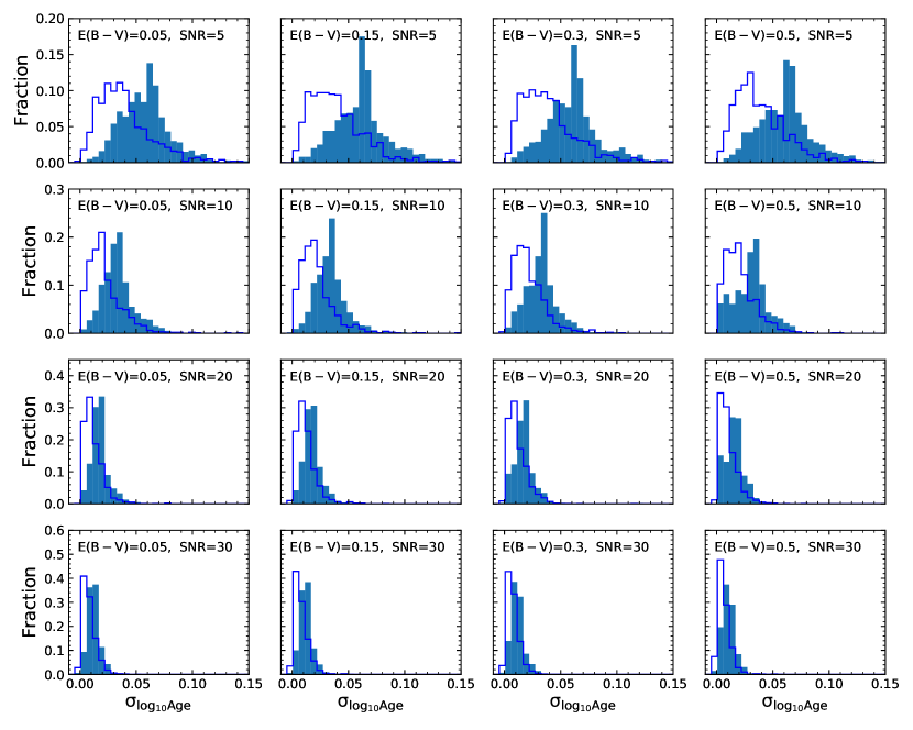
Figure 33: Histograms of uncertainty of stellar age in stellar population synthesis (SPS), as quantified by $\sigma_{\log_{10}{\rm Age}}$ which is the $1-\sigma$ width of the posterior distribution of $\log_{10}{\rm Age}$ inferred by fitting the mock spectra with our SPS code BIGS. Different panels are for different $E(B-V)$ and signal-to-noise ratios (SNSs), as indicated. In each panel the filled histogram is for the case where $E(B-V)$ is a free parameter and constrained simultenously with other stellar population properties during the spectral fitting, while the unfilled histogram is for the case where the spectrum being considered is corrected for dust attenuation using our method before the fitting.

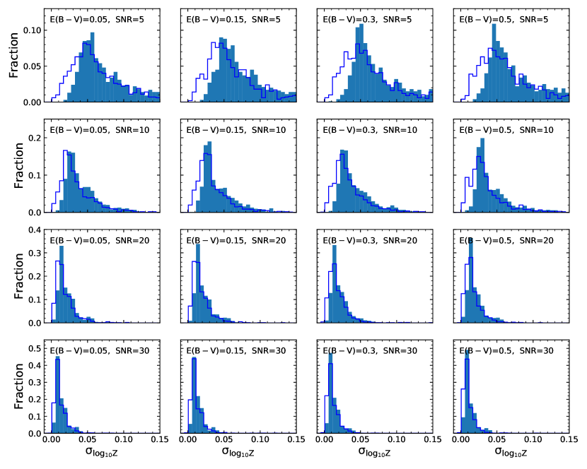
Figure 34: Same as Fig. 33 but for stellar metallicity instead of stellar age.

Appendix B Alleviating the degeneracy between dust and stellar populations

As emphasized in the main text, one important advantage of our method is that the estimated (relative) dust attenuation curves are independent of the shape of theoretical attenuation curves. The method provides a reliable and direct way to estimate the attenuation curve and to correct the effect of attenuation for the observed spectrum, thereby avoiding dust attenuation in stellar population synthesis (SPS) modeling. In principle, this should also help break the degeneracy between dust, age and metallicity in observed spectra. Here we present a test of this hypothesis using the same set of mock spectra generated in the previous section. For this purpose, we use our recently developed SPS code, Bayesian Inference of Galactic Spectra (BIGS, Zhou et al., 2019). The code performs full spectral fitting to the observed spectrum of a galaxy (or a region within it), and derives Bayesian inferences of age and metallicty along with other properties of its stellar population. In particular, the Bayesian approach provides a statistically rigorous way to explore potential degeneracy among model parameters.

For simplicity, we consider only mock spectra with emission lines. We first apply BIGS to each of the mock spectra and obtain the corresponding posterior distribution of stellar population properties, such as age, metallicity and $E(B-V)$. Next, we apply our method to estimate the dust attenuation and to correct the effect of attenuation. Finally, we use BIGS to fit the ‘dust-free’ spectrum. Figs. 33 and 34 show the $1-\sigma$ width of the posterior distribution of stellar age ($\sigma_{\log_{10}{\rm Age}}$) and metallicity ($\sigma_{\log_{10}{\rm Z}}$), for different $E(B-V)$ and SNR. In each panel, the filled histogram is the result obtained from applying BIGS directly to the mock spectra, with dust attenuation treated as a free parameter during the fitting. The unfilled histogram is the result of fitting the spectra in which dust attenuation is estimated and corrected using our method. As one can see, in all cases the inference uncertainties for both of the stellar parameters are reduced when the dust attenuation is corrected before the fitting. The improvement is more pronounced for lower SNRs, but with week or no dependence on $E(B-V)$. These results confirm the above hypothesis and motivate applications of our method of modeling attenuation and BIGS to real spectra of galaxies (N. Li et al., in prep.).

References

- Abazajian et al. (2003) Abazajian, K., Adelman-McCarthy, J. K., Agüeros, M. A., et al. 2003, AJ, 126, 2081, doi: 10.1086/378165
- Abolfathi et al. (2018) Abolfathi, B., Aguado, D. S., Aguilar, G., et al. 2018, ApJS, 235, 42, doi: 10.3847/1538-4365/aa9e8a
- Battisti et al. (2017a) Battisti, A. J., Calzetti, D., & Chary, R.-R. 2017a, ApJ, 840, 109, doi: 10.3847/1538-4357/aa6fb2
- Battisti et al. (2017b) —. 2017b, ApJ, 851, 90, doi: 10.3847/1538-4357/aa9a43
- Blanton et al. (2017) Blanton, M. R., Bershady, M. A., Abolfathi, B., et al. 2017, AJ, 154, 28, doi: 10.3847/1538-3881/aa7567
- Bruzual & Charlot (2003) Bruzual, G., & Charlot, S. 2003, MNRAS, 344, 1000, doi: 10.1046/j.1365-8711.2003.06897.x
- Bundy et al. (2015) Bundy, K., Bershady, M. A., Law, D. R., et al. 2015, ApJ, 798, 7, doi: 10.1088/0004-637X/798/1/7
- Calzetti et al. (2000) Calzetti, D., Armus, L., Bohlin, R. C., et al. 2000, ApJ, 533, 682, doi: 10.1086/308692
- Calzetti et al. (1994) Calzetti, D., Kinney, A. L., & Storchi-Bergmann, T. 1994, ApJ, 429, 582, doi: 10.1086/174346
- Cappellari (2017) Cappellari, M. 2017, MNRAS, 466, 798, doi: 10.1093/mnras/stw3020
- Cappellari & Emsellem (2004) Cappellari, M., & Emsellem, E. 2004, PASP, 116, 138, doi: 10.1086/381875
- Cardelli et al. (1989) Cardelli, J. A., Clayton, G. C., & Mathis, J. S. 1989, ApJ, 345, 245, doi: 10.1086/167900
- Chabrier (2003) Chabrier, G. 2003, PASP, 115, 763, doi: 10.1086/376392
- Charlot & Fall (2000) Charlot, S., & Fall, S. M. 2000, ApJ, 539, 718, doi: 10.1086/309250
- Chevallard & Charlot (2016) Chevallard, J., & Charlot, S. 2016, MNRAS, 462, 1415, doi: 10.1093/mnras/stw1756
- Cid Fernandes et al. (2005) Cid Fernandes, R., Mateus, A., Sodré, L., Stasińska, G., & Gomes, J. M. 2005, MNRAS, 358, 363, doi: 10.1111/j.1365-2966.2005.08752.x
- Conroy (2013) Conroy, C. 2013, ARA&A, 51, 393, doi: 10.1146/annurev-astro-082812-141017
- de Grijs et al. (1997) de Grijs, R., Peletier, R. F., & van der Kruit, P. C. 1997, A&A, 327, 966
- Decleir et al. (2019) Decleir, M., De Looze, I., Boquien, M., et al. 2019, MNRAS, 486, 743, doi: 10.1093/mnras/stz805
- Deeming (1964) Deeming, T. J. 1964, MNRAS, 127, 493, doi: 10.1093/mnras/127.6.493
- Drory et al. (2015) Drory, N., MacDonald, N., Bershady, M. A., et al. 2015, AJ, 149, 77, doi: 10.1088/0004-6256/149/2/77
- Fitzpatrick (1999) Fitzpatrick, E. L. 1999, PASP, 111, 63, doi: 10.1086/316293
- Ge et al. (2018) Ge, J., Yan, R., Cappellari, M., et al. 2018, MNRAS, 478, 2633, doi: 10.1093/mnras/sty1245
- Gordon et al. (2003) Gordon, K. D., Clayton, G. C., Misselt, K. A., Landolt, A. U., & Wolff, M. J. 2003, ApJ, 594, 279, doi: 10.1086/376774
- Gordon et al. (2000) Gordon, K. D., Clayton, G. C., Witt, A. N., & Misselt, K. A. 2000, ApJ, 533, 236, doi: 10.1086/308668
- Johnson et al. (2013) Johnson, S. P., Wilson, G. W., Tang, Y., & Scott, K. S. 2013, MNRAS, 436, 2535, doi: 10.1093/mnras/stt1758
- Law et al. (2016) Law, D. R., Cherinka, B., Yan, R., et al. 2016, AJ, 152, 83, doi: 10.3847/0004-6256/152/4/83
- Leitherer et al. (1999) Leitherer, C., Schaerer, D., Goldader, J. D., et al. 1999, ApJS, 123, 3, doi: 10.1086/313233
- Li et al. (2005) Li, C., Wang, T.-G., Zhou, H.-Y., Dong, X.-B., & Cheng, F.-Z. 2005, AJ, 129, 669, doi: 10.1086/426909
- Maraston (2005) Maraston, C. 2005, MNRAS, 362, 799, doi: 10.1111/j.1365-2966.2005.09270.x
- Markwardt (2009) Markwardt, C. B. 2009, in Astronomical Society of the Pacific Conference Series, Vol. 411, Astronomical Data Analysis Software and Systems XVIII, ed. D. A. Bohlender, D. Durand, & P. Dowler, 251. https://arxiv.org/abs/0902.2850
- Meurer et al. (1999) Meurer, G. R., Heckman, T. M., & Calzetti, D. 1999, ApJ, 521, 64, doi: 10.1086/307523
- Mo et al. (2010) Mo, H., van den Bosch, F. C., & White, S. 2010, Galaxy Formation and Evolution
- Narayanan et al. (2018) Narayanan, D., Conroy, C., Davé, R., Johnson, B. D., & Popping, G. 2018, ApJ, 869, 70, doi: 10.3847/1538-4357/aaed25
- Noll et al. (2009) Noll, S., Burgarella, D., Giovannoli, E., et al. 2009, A&A, 507, 1793, doi: 10.1051/0004-6361/200912497
- Ocvirk et al. (2006a) Ocvirk, P., Pichon, C., Lançon, A., & Thiébaut, E. 2006a, MNRAS, 365, 46, doi: 10.1111/j.1365-2966.2005.09182.x
- Ocvirk et al. (2006b) —. 2006b, MNRAS, 365, 74, doi: 10.1111/j.1365-2966.2005.09323.x
- Osterbrock & Ferland (2006) Osterbrock, D. E., & Ferland, G. J. 2006, Astrophysics of gaseous nebulae and active galactic nuclei
- Prevot et al. (1984) Prevot, M. L., Lequeux, J., Maurice, E., Prevot, L., & Rocca-Volmerange, B. 1984, A&A, 132, 389
- Reddy et al. (2015) Reddy, N. A., Kriek, M., Shapley, A. E., et al. 2015, ApJ, 806, 259, doi: 10.1088/0004-637X/806/2/259
- Salim & Boquien (2019) Salim, S., & Boquien, M. 2019, ApJ, 872, 23, doi: 10.3847/1538-4357/aaf88a
- Salim et al. (2018) Salim, S., Boquien, M., & Lee, J. C. 2018, ApJ, 859, 11, doi: 10.3847/1538-4357/aabf3c
- Salmon et al. (2016) Salmon, B., Papovich, C., Long, J., et al. 2016, ApJ, 827, 20, doi: 10.3847/0004-637X/827/1/20
- Takada et al. (2014) Takada, M., Ellis, R. S., Chiba, M., et al. 2014, PASJ, 66, R1, doi: 10.1093/pasj/pst019
- Tojeiro et al. (2007) Tojeiro, R., Heavens, A. F., Jimenez, R., & Panter, B. 2007, MNRAS, 381, 1252, doi: 10.1111/j.1365-2966.2007.12323.x
- Tress et al. (2018) Tress, M., Mármol-Queraltó, E., Ferreras, I., et al. 2018, MNRAS, 475, 2363, doi: 10.1093/mnras/stx3334
- Vazdekis et al. (2010) Vazdekis, A., Sánchez-Blázquez, P., Falcón-Barroso, J., et al. 2010, MNRAS, 404, 1639, doi: 10.1111/j.1365-2966.2010.16407.x
- Wake et al. (2017) Wake, D. A., Bundy, K., Diamond-Stanic, A. M., et al. 2017, AJ, 154, 86, doi: 10.3847/1538-3881/aa7ecc
- Wild et al. (2011) Wild, V., Charlot, S., Brinchmann, J., et al. 2011, MNRAS, 417, 1760, doi: 10.1111/j.1365-2966.2011.19367.x
- Wilkinson et al. (2017) Wilkinson, D. M., Maraston, C., Goddard, D., Thomas, D., & Parikh, T. 2017, MNRAS, 472, 4297, doi: 10.1093/mnras/stx2215
- Wilkinson et al. (2015) Wilkinson, D. M., Maraston, C., Thomas, D., et al. 2015, MNRAS, 449, 328, doi: 10.1093/mnras/stv301
- Yan et al. (2016a) Yan, R., Tremonti, C., Bershady, M. A., et al. 2016a, AJ, 151, 8, doi: 10.3847/0004-6256/151/1/8
- Yan et al. (2016b) Yan, R., Bundy, K., Law, D. R., et al. 2016b, AJ, 152, 197, doi: 10.3847/0004-6256/152/6/197
- Yuan et al. (2018) Yuan, F.-T., Argudo-Fernández, M., Shen, S., et al. 2018, A&A, 613, A13, doi: 10.1051/0004-6361/201731865
- Zhou et al. (2019) Zhou, S., Mo, H. J., Li, C., et al. 2019, MNRAS, 485, 5256, doi: 10.1093/mnras/stz764