On the construction of non-Hermitian Hamiltonians with all-real spectra through supersymmetric algorithms

Abstract

The energy spectra of two different quantum systems are paired through supersymmetric algorithms. One of the systems is Hermitian and the other is characterized by a complex-valued potential, both of them with only real eigenvalues in their spectrum. The superpotential that links these systems is complex-valued, parameterized by the solutions of the Ermakov equation, and may be expressed either in nonlinear form or as the logarithmic derivative of a properly chosen complex-valued function. The non-Hermitian systems can be constructed to be either parity-time-symmetric or non-parity-time-symmetric.

1 Introduction

The supersymmetric formulation of quantum mechanics is a subject of intense activity in contemporary physics. It is addressed to analyze the spectral properties of exactly solvable potentials as well as to construct new integrable quantum models [1, 2, 3]. Sustained by the factorization method [4, 5], the supersymmetric approach is basically algebraic [6] and permits the pairing between the spectrum of a given (well-known) Hamiltonian $H_{0}$ to the spectrum of a second (generally unknown) Hamiltonian $H_{1}$. In terms of differential operators, it has been found that the factorization of either $H_{0}$ or $H_{1}$ is not unique [4] and that the pairing of $H_{0}$ with $H_{1}$ is ruled by a Darboux transformation [7], which was introduced in 1882 [8] (see historical details in e.g. [3, 9]). The keystone is a solution $u$ (not necessarily normalizable) of the eigenvalue equation $H_{0}u=\epsilon u$ that is used to generate the Darboux transformation $V_{1}(x)=V_{0}(x)+2\frac{d}{dx}\beta(x)$ [4, 5], where $\beta(x)=-\frac{d}{dx}\ln u(x)$ is called superpotential and $\epsilon$ the factorization energy. Remarkably, not only Hermitian but also non-Hermitian Hamiltonians $H_{1}$ can be produced as supersymmetric partners of a given exactly solvable (either Hermitian or non-Hermitian) Hamiltonian $H_{0}$. Indeed, depending on the properties of $V_{0}(x)$ and $\beta(x)$, the new potential $V_{1}(x)$ may be either real or complex-valued. In any case, the spectrum of the new Hamiltonian $H_{1}$ includes either all-real eigenvalues or a combination of real and complex eigenvalues, see e.g. [10, 11, 12, 13, 14, 15, 16, 17, 18, 19, 20, 21, 22, 23].

Quite recently, a complex-valued superpotential defined by the nonlinear expression

$$\beta(x)=-\frac{d}{dx}\ln\alpha^{\prime}(x)+i\frac{\lambda}{\alpha^{2}(x)},\quad\lambda\in\mathbb{R},$$ (1)

has been provided to produce new classes of non-Hermitian Hamiltonians $H_{1}$ with all-real spectra [19]. The function $\alpha(x)$ is a solution of the Ermakov equation [24]:

$$-\frac{d^{2}}{dx^{2}}\alpha(x)+V_{0}(x)\alpha(x)=\epsilon\alpha(x)+\frac{\lambda^{2}}{\alpha^{3}(x)},$$ (2)

which is reduced to the eigenvalue equation $H_{0}\alpha=\epsilon\alpha$ for $\lambda=0$. The eigenfunctions of the resulting non-Hermitian Hamiltonians $H_{1}$ satisfy some properties of interlacing of zeros that permit the study of the related systems as if they were Hermitian [20]. Indeed, a bi-orthogonal basis can be introduced to facilitate the construction of coherent states for such a class of systems [21]. Moreover, the factorization energy $\epsilon$ can be positioned at any arbitrary position in the spectrum of $H_{1}$ [22]. Notedly, the eigenvalues of the non-Hermitian Hamiltonians $H_{1}$ are all-real regardless of whether $H_{1}$ is parity-time-symmetric [25] or not.

In this communication we briefly revisit the method developed in [19, 20, 21, 22] and show that the nonlinear superpotential (1) can be also expressed in the ‘canonical form’ $\beta(x)=-\frac{d}{dx}\ln u(x)$, where $u$ is an eigenfunction of $H_{0}$ with very concrete profile. The results presented here generalize the approach introduced in [11], where it is guessed that a complex linear-combination of eigenfunctions of $H_{0}$ may be useful to construct complex-valued potentials $V_{1}(x)$. We provide a pair of examples where the new potentials are either parity-time-symmetric or non-parity-time-symmetric.

2 Factorization method and non-Hermitian Hamiltonians

Consider an initial Hamiltonian

$$H_{0}=-\frac{d^{2}}{dx^{2}}+V_{0}(x),$$ (3)

with $V_{0}(x)$ a real-valued potential defined in $\mbox{Dom}V_{0}\subseteq\mathbb{R}$. We assume that the energy eigenvalues $E^{(0)}\in\mathbb{R}$ and eigenfunctions $\phi(x)$ of the related eigenvalue equation $H_{0}\phi(x)=E^{(0)}\phi(x)$ are already known. In particular, the bounded solutions $\phi_{n}(x)$ belong to the discrete eigenvalues $E_{n}^{(0)}$, $n=0,1,\ldots$ Let us introduce a pair of non-mutually adjoint operators, $A$ and $B$, such that

$$H_{0}=AB+\epsilon,\quad A=-\frac{d}{dx}+\beta(x),\quad B=\frac{d}{dx}+\beta(x),$$ (4)

where $\beta(x)$ is in general a complex-valued function and $\epsilon$ is a real constant. After comparing (4) with (3) one arrives at the Riccati equation

$$-\beta^{\prime}+\beta^{2}=V_{0}(x)-\epsilon,\quad\beta^{\prime}=\frac{d\beta}{dx}.$$ (5)

Provided a solution of (5), reversing the order of the factors in (4) gives

$$H_{1}=BA+\epsilon=-\frac{d^{2}}{dx^{2}}+V_{1}(x),\quad V_{1}(x)=V_{0}(x)+2\beta^{\prime}(x).$$ (6)

Notice that the new operator $H_{1}$ is not self-adjoint since $V_{1}$ is complex-valued in general. Indeed, $H_{1}^{\dagger}=A^{\dagger}B^{\dagger}+\epsilon=-\frac{d^{2}}{dx^{2}}+V_{1}^{*}\neq H_{1}$. Nevertheless, the pair $H_{0}$ and $H_{1}$ satisfies the intertwining relationships

$$BH_{0}=H_{1}B,\quad H_{0}A=AH_{1},$$ (7)

so that the eigenvalue equation $H_{1}\psi_{n}=E_{n}^{(1)}\psi_{n}$, $n=0,1,\ldots$, is automatically solved by the set

$$\psi_{n+1}=\frac{1}{\sqrt{E_{n}^{(0)}-\epsilon}}B\phi_{n}\,,\quad A\psi_{0}=0\,,\quad E_{n+1}^{(1)}=E_{n}^{(0)}\,,\quad E_{0}^{(1)}=\epsilon\,.$$ (8)

The functions $\psi_{n}(x)$ are complex-valued and such that the zeros of their real and imaginary parts satisfy some theorems of interlacing [20].

2.1 Complex-valued potentials with all-real spectra

In the conventional supersymmetric approaches the solution of the Riccati equation (5) is usually taken to be real-valued. However, complex-valued solutions are feasible even for real-valued potentials $V_{0}$ and real factorization energies $\epsilon$. Indeed, the real and imaginary parts of Eq. (5) lead to a coupled system which is solved by the complex-valued superpotential (1). Assuming, with no loss of generality, that $\alpha(x)$ is real-valued, it may be shown that the solution of the Ermakov (2) can be written as [19]:

$$\alpha(x)=\left[au_{1}^{2}(x)+bu_{1}(x)u_{2}(x)+cu_{2}^{2}(x)\right]^{1/2},$$ (9)

where $u_{1,2}$ are solutions of the system

$$-u_{1,2}^{\prime\prime}+V_{0}u_{1,2}=\epsilon u_{1,2},\quad W(u_{1},u_{2})=u_{1}u_{2}^{\prime}-u_{1}^{\prime}u_{2}=W_{0},$$ (10)

with $W_{0}=\mbox{const}$. The function $\alpha$ is free of zeros in $\mbox{Dom}V_{0}$ if the set $\{a,b,c\}$ is integrated by positive numbers that are constrained as follows

$$b^{2}-4ac=-4\lambda^{2}/W_{0}^{2}.$$ (11)

Using the superpotential (1), with $\alpha$ given in (9), the new potential (6) is now given by the nonlinear expression

$$V_{1}(x)=V_{0}(x)-2\left(\ln\alpha(x)\right)^{\prime\prime}+i\left(\frac{2\lambda}{\alpha^{2}(x)}\right)^{\prime},\quad\lambda\in\mathbb{R}.$$ (12)

Notice that the results of the conventional supersymmetric approaches [1, 2, 3] are automatically recovered for $\lambda=0$. On the other hand, it may be shown that the imaginary part of $V_{1}(x)$ satisfies the condition of zero total area [20]:

$$\int_{DomV_{0}}\mbox{Im}V_{1}(x)dx=\left.\frac{2\lambda}{\alpha^{2}(x)}\right|_{DomV_{0}}=0,$$ (13)

so that the total probability is conserved. The latter means that the potentials (12) can be addressed to represent open quantum systems with balanced gain (acceptor) and loss (donor) profile [26].

2.1.1 Parity-time-symmetric potentials

Potentials featuring the parity-time symmetry [25] represent a particular case of the applicability of the condition of zero total area (13). Such potentials are invariant under parity (P) and time‐reversal (T) transformations in quantum mechanics, so that a necessary condition for PT-symmetry is $V(x)=V^{*}(-x)$, where ^∗ stands for complex conjugation. For initial potentials $V_{0}(x)$ such that $V_{0}(x)=V_{0}(-x)$, one can show that making $b=0$ in (9) is sufficient to get $V_{1}^{*}(x)=V^{*}_{1}(-x)$. In other words, the parity-time symmetry is a consequence of the condition of zero total area in our approach.

2.1.2 Non-parity-time-symmetric potentials

For $V_{0}(x)\neq V_{0}(-x)$ the property $V_{1}^{*}(x)=V^{*}_{1}(-x)$ does not hold anymore, so the complex-valued potentials (12) have all-real spectra although they are non-parity-symmetric. Diverse examples have been already discussed in e.g. [19, 20, 21, 22]. Quite recently the pseudo-Hermiticity and supersymmetric approaches have been combined to get new classes of non-parity-time-symmetric potentials with all-real spectra [23]. Interestingly, such potentials can be manipulated to induce phase transitions where conjugate pairs of complex eigenvalues emerge in the spectrum. Similar results have been reported in [27], where the condition of zero total area (13) plays a relevant role. The discussion on the subject is out of the scope of the present work and will be reported elsewhere.

2.2 Recovering the canonical form of the superpotential

We wonder if the nonlinear expression (1) can be reduced to the canonical form $\beta=-\frac{d}{dx}\ln u(x)$. Keeping this in mind, we first rewrite (1) as

$$\beta=-\frac{\frac{1}{2}(\alpha^{2})^{\prime}-i\lambda}{\alpha^{2}}.$$ (14)

Using (9) and (11) we factorize the $\alpha$-function in the form

$$\alpha^{2}=\frac{1}{a}\left[au_{1}+\left(\frac{b}{2}+i\frac{\lambda}{W_{0}}\right)u_{2}\right]\left[au_{1}+\left(\frac{b}{2}-i\frac{\lambda}{W_{0}}\right)u_{2}\right].$$ (15)

In turn, expanding the numerator of Eq. (14) yields

$$\frac{1}{2}\left(\alpha^{2}\right)^{\prime}-i\lambda=au_{1}u_{1}^{\prime}+cu_{2}u_{2}^{\prime}+bu_{1}^{\prime}u_{2}+\left(\frac{bW_{0}}{2}-i\lambda\right),$$ (16)

where we have used the Wronskian defined in (10). The latter result is now factorized:

$$(C_{0}u_{1}^{\prime}+C_{1}u_{2}^{\prime})(D_{0}u_{1}+D_{1}u_{2}).$$ (17)

The coefficients $C_{0},C_{1},D_{0},D_{1}$ are defined by comparing the expanded version of (17) with (16). One gets

$$\frac{1}{2}\left(\alpha^{2}\right)^{\prime}-i\lambda=\frac{1}{a}\left[au_{1}^{\prime}+\left(\frac{b}{2}-i\frac{\lambda}{W_{0}}\right)u_{2}^{\prime}\right]\left[au_{1}+\left(\frac{b}{2}+i\frac{\lambda}{W_{0}}\right)u_{2}\right]\,.$$ (18)

Finally, the substitution of (15) and (18) into (14) produces

$$\beta=-\frac{\alpha^{\prime}(x)}{\alpha(x)}+i\frac{\lambda}{\alpha^{2}(x)}=-\frac{d}{dx}\ln\left[au_{1}+\left(\frac{b}{2}-i\frac{\lambda}{W_{0}}\right)u_{2}\right].$$ (19)

Thus, the function we are looking for is given by the linear superposition

$$u=au_{1}+\left(\frac{b}{2}-i\frac{\lambda}{W_{0}}\right)u_{2},$$ (20)

where the constants $a$, $b$ and $\lambda$ are linked by the condition (11). If $\lambda=0$ the constraint (11) becomes $b=\pm 2\sqrt{ac}$, so that the coefficients of the superposition (20) are real numbers, $u=\sqrt{a}\left(\sqrt{a}u_{1}+\sqrt{c}u_{2}\right)$, as expected.

The expression (19) shows that the superpotential $\beta(x)$ can be written in either the nonlinear form (1), or as the logarithmic derivative of the function $u$ defined in (20). The latter is a linear superposition of the solutions of (10) with complex coefficients that are uniquely defined by the condition (11). Notice that the derivation of the $u$-function (20) generalizes the approach introduced in [11], where it is guessed that a linear combination of $u_{1,2}$ would give rise to complex-valued potentials $V_{1}$ whenever the appropriate complex coefficients have been included. As an example, in [11] the authors provide the coefficients that produce a family of oscillator-like complex-valued potentials. They also apply their method to study the potential $V_{1}(x)=-\tfrac{1}{2}(ix)^{N}$, $N\geq 2$, introduced in [25], and describe some other potentials that can be studied within their approach. However, no general rule to fix the appropriate complex coefficients is given in [11]. In contrast, the linear superposition (20) is general in the sense that the rule (11) applies for any differentiable and exactly solvable real-valued initial potential $V_{0}(x)$. Diverse examples have been already provided in [19, 20, 21, 22].

3 Examples and discussion of results

As immediate examples let us discuss the regular complex-valued potential $V_{1}(x)$ generated by the following initial potentials:

$\bullet$ Free particle. Given $V_{0}(x)=0$, the basis set is $u_{1}=e^{ikx}$ and $u_{2}=e^{-ikx}$, with $W_{0}=-2ik$. To get a real-valued $\alpha$-function we take $k=i\frac{\kappa}{2}$, with $\kappa>0$. Without loosing generality we now make $a=c$. Then,

$$\alpha(x)=\left[2a\cosh\kappa x+b\right]^{1/2},\qquad u(x)=ae^{-\kappa x/2}+\left(\frac{b}{2}-i\frac{\lambda}{\kappa}\right)e^{\kappa x/2}.$$ (21)

The potentials $V_{1}(x)$ are depicted in Fig. 1, they are of the Pöschl-Teller type, generalize the well known family of regular (real-valued) supersymmetric partners of the free particle [28], and satisfy the condition of zero total area (13). These potentials include only one bound state of energy $E^{(0)}=-\tfrac{1}{4}\kappa^{2}$. The effect of $b\neq 0$ is to slide the potential to the right (red curve in Figure 1), so that $V_{1}(x)$ is parity-time-invariant after the appropriate shift. The latter is just because the initial potential $V_{0}(x)=0$ satisfies the condition $V_{0}(x)=V_{0}(-x)$ and exhibits, at the same time, translational symmetry $V_{0}(x)=V_{0}(x+x_{0})$. One may say that, in the present case, the translational symmetry is invariant under the Darboux transformations (12).

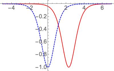
(a) $\mbox{Re}V_{1}(x)$

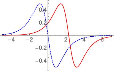
(b) $\mbox{Im}V_{1}(x)$

Figure 1: The real and imaginary parts of the complex-valued potentials with all-real spectra (12) derived from the expressions of the free particle provided in (21) with $b\neq 0$, $a=1.5$ (red curve), and $b=0$, $a=1$ (dotted-blue curve). In all cases $\lambda=\kappa=1$.

$\bullet$ Morse potential. It is clear that the condition $V_{0}(x)=V_{0}(-x)$ cannot be applied on the Morse potential

$$V_{0}(x)=\Gamma_{0}(1-e^{-\gamma x})^{2},\quad x\in\mathbb{R}.$$ (22)

Then, the potentials (12) associated to (22) are non-parity-time-symmetric for any values of the set $\{a,b,c\}$. The condition $\Gamma_{0}>\gamma^{2}/2$ ensures that at least one bound state exists. It may be shown [22] that two linear independent solutions of (10) for $\epsilon\in\mathbb{R}$ are given in terms of confluent hypergeometric functions as follows

$$u_{1}(x)=e^{-y/2}y^{\sigma}{}_{1}F_{1}\left(\sigma+\frac{1}{2}-d;1+2\sigma;y\right),$$ (23)

$$u_{2}(x)=e^{-y/2}y^{-\sigma}{}_{1}F_{1}\left(-\sigma+\frac{1}{2}-d;1-2\sigma;y\right),$$

where

$$y=2de^{-\gamma x},\quad d^{2}=\frac{\Gamma_{0}}{\gamma^{2}},\quad\sigma^{2}=\frac{\Gamma_{0}-\epsilon}{\gamma^{2}},\quad W_{0}=2\sqrt{\Gamma_{0}-\epsilon}.$$ (24)

The physical energy eigenvalues are given by

$$E_{n}=\gamma\left[(2n+1)\sqrt{\Gamma_{0}}-\gamma(n+1/2)^{2}\right],\quad n=0,1,\ldots N,$$ (25)

where $N$ is given by the floor function $N=\lfloor\frac{\sqrt{\Gamma_{0}}}{\gamma}-\frac{1}{2}\rfloor$. The related eigenfunctions can be recovered from (23) after substituting $E_{n}$ for $\epsilon$ and the appropriate boundary conditions. In Fig. 2 we show the potential (22) and two of its supersymmetric partners for $\gamma=1$ and $\Gamma_{0}=4$. In such case, the initial potential admits two bound states with energy eigenvalues $E_{0}^{(0)}=7/4$ and $E_{1}^{(0)}=15/4$. Notice that, besides the above energies, potentials $V_{1}(x)$ include the eigenvalue $E_{0}^{(1)}=\epsilon=1$ in their spectra. Moreover, they satisfy the condition of zero total area (13).

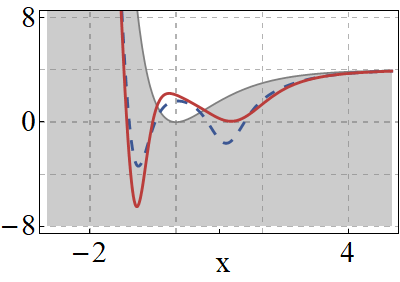
(a) $\mbox{Re}V_{1}(x)$

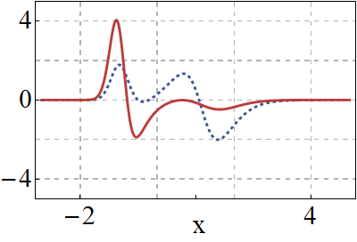
(b) $\mbox{Im}V_{1}(x)$

Figure 2: The real and imaginary parts of the complex-valued potential with all-real spectra (12) derived for the expressions of the Morse potential provided in (23) with $a=c=1$ (red curve), and $a=1$, $c=1/3$, $b=0$ (dotted-blue curve). In all cases $\lambda=2$ and $\epsilon=1$. The gray area delimitates the initial Morse potential.

In summary, the method introduced in [19] and developed in [20, 21, 22] provides complex-valued potentials with all-real spectra that includes the parity-time-symmetric case as a particular result. The keystone of the approach relies on the solutions to the Ermakov equation (2) and the nonlinearity of the imaginary part of the superpotential (1). The latter permits to introduce the constraint (11) as an universal rule to choice the complex parameters that are required in the superposition (20) to get properly defined complex potentials in supersymmetric quantum mechanics.

Acknowledgment

This research was funded by Consejo Nacional de Ciencia y Tecnología (Mexico), grant number A1-S-24569, and by Instituto Politécnico Nacional (Mexico), project SIP20195981. K. Zelaya acknowledges the support from the Mathematical Physics Laboratory, Centre de Recherches Mathématiques, through a postdoctoral fellowship.

References

- [1] B.K. Bagchi, Supersymmetry in Quantum and Classical Mechanics, Chapman and Hall, CRC press, London, Boca Raton, 2000.
- [2] F. Cooper, A. Khare and U. Sukhatme, Supersymmetry in Quantum Mechanics, World Scientific, Singapore, 2001.
- [3] B. Mielnik and O. Rosas‐Ortiz, Factorization: little or great algorithm?, J. Phys. A: Math. Gen. 37 (2004) 10007.
- [4] B. Mielnik, Factorization method and new potentials with the oscillator spectrum, J. Math. Phys. 25 (1984) 3387.
- [5] A.A. Andrianov, N.V. Borisov and M.V. Ioffe, The factorization method and quantum systems with equivalent energy spectra, Phys. Lett. A 105 (1984) 19
- [6] A.A. Andrianov, N.V. Borisov, M.V. Ioffe and M.L. Eides, Supersymmetric mechanics: a new look at the equivalence of quantum systems, Theor. Math. Phys. 61 (1984) 965.
- [7] A.A. Andrianov, N.V. Borisov and M.V. Ioffe, Factorization method and Darboux transformation for multidimensional Hamiltonians, Theor. Math. Phys. 61 (1984) 1078.
- [8] G. Darboux, Sur une proposition relative aux q́uations linéares, C.R. Acad. Sci. Paris 94 (1882) 1456.
- [9] H. Rosu, Short survey of Darboux transformations, in Proceedings of the First International Workshop on Symmetries in Quantum Mechanics and Quantum Optics, A. Ballesteros et.al. (Eds), Servicio de Publicaciones de la Universidad de Burgos, 1999, pp. 301
- [10] D. Baye, G. Lévai and J.M. Sparenberg, Phase-equivalent complex potentials, Nucl. Phys. A 599 (1996) 435.
- [11] F. Cannata, G. Junker and J.Trost, Schrödinger operators with complex potential but real spectrum, Phys. Lett. A (1998) 246 219
- [12] A.A. Andrianov, M.V. Ioffe, F. Cannata and J.P. Dedonder, Susy quantum mechanics with complex superpotentials and real energy spectra, Int. J. Mod. Phys. A (1999) 14 2675.
- [13] B. Bagchi, S. Mallik and C. Quesne, Generating complex potentials with real eigenvalues in supersymmetric quantum mechanics, Int. J. Mod. Phys. A (2001) 16 2859
- [14] O. Rosas-Ortiz and R. Muñoz, Non-Hermitian SUSY hydrogen-like Hamiltonians with real spectra, J. Phys. A: Math. Gen. 36 (2003) 8497.
- [15] O. Rosas-Ortiz, Gamow vectors and supersymmetric quantum mechanics, Rev. Mex. Fis. 53 (2007) 103.
- [16] N. Fernández-García and O. Rosas-Ortiz, Optical potentials using resonance states in Supersymmetric Quantum Mechanics, J. Phys. Conf. Ser. 128 (2008) 012044.
- [17] N. Fernández-García and O. Rosas-Ortiz O, Gamow–Siegert functions and Darboux-deformed short range potentials, Ann. Phys. (2008) 323 1397.
- [18] M. Miri, M. Heinrich and D.N. Christodoulides, Supersymmetry-generated complex optical potentials with real spectra, Phys. Rev. A 87 (2013) 043819.
- [19] O. Rosas-Ortiz, O Castaños and D. Schuch, New supersymmetry-generated complex potentials with real spectra, J. Phys. A: Math. Theor. 48 (2015) 445302.
- [20] A. Jaimes-Najera and O. Rosas-Ortiz, Interlace properties for the real and imaginary parts of the wave functions of complex-valued potentials with real spectrum, Ann. Phys. 376 (2017) 126.
- [21] O. Rosas-Ortiz and K. Zelaya, Bi-Orthogonal Approach to Non-Hermitian Hamiltonians with the Oscillator Spectrum: Generalized Coherent States for Nonlinear Algebras, Ann. Phys. 388 (2018) 26.
- [22] Z. Blanco-Garcia, O. Rosas-Ortiz and K. Zelaya, Interplay between Riccati, Ermakov and Schrödinger equations to produce complex-valued potentials with real energy spectrum, Math. Meth. Appl. Sci. 42 (2019) 4925.
- [23] B. Bagchi and J. Yang, New families of non-parity-time-symmetric complex potentials with all-real spectra, arXiv:1908.03758
- [24] V. Ermakov, Second order differential equations. Conditions of complete integrability, Kiev University Izvestia, Series III 9 (1880) 1 (in Russian). English translation by A.O. Harin, Appl Anal Discrete Math. 2 (2008) 123.
- [25] C. M. Bender and S. Boettcher, Real spectra in non-Hermitian Hamiltonians having PT-symmetry, Phys. Rev. Lett. 80 (1998) 5243.
- [26] H. Eleuch and I. Rotter, Gain and loss in open quantum systems, Phys Rev E. 95 (2017) 062109.
- [27] A. Jaimes-Najera, Oscillation theorems and dynamics for Hermitian and non-Hermitian Hamiltonians in Quantum Mechanics, PhD Thesis, Physics Department, Cinvestav, 2016.
- [28] B. Mielnik, L.M. Nieto and O. Rosas-Ortiz, The finite difference algorithm for higher order supersymmetry, Phys. Lett. A 269 (2000) 70.