Locating conical degeneracies in the spectra of parametric self-adjoint matrices

Abstract.

A simple iterative scheme is proposed for locating the parameter values for which a 2-parameter family of real symmetric matrices has a double eigenvalue. The convergence is proved to be quadratic. An extension of the scheme to complex Hermitian matrices (with 3 parameters) and to location of triple eigenvalues (5 parameters for real symmetric matrices) is also described. Algorithm convergence is illustrated in several examples: a real symmetric family, a complex Hermitian family, a family of matrices with an “avoided crossing” (no convergence) and a 5-parameter family of real symmetric matrices with a triple eigenvalue.

1. Introduction

A theorem of von Neumann and Wigner states that, generically, a two-parameter family of real symmetric matrices has multiple eigenvalues at isolated points [29]. In other words, the matrices with multiple eigenvalues have co-dimension 2 in the manifold of real symmetric matrices [1, Appendix 10]. In this paper, we would like to address the problem of locating these isolated points of eigenvalue multiplicity in the 2-dimensional parameter space. To be more precise, we consider the following problem.

Problem.

Given a smooth real symmetric matrix valued function $A:\mathbb{R}^{2}\mapsto\mathbb{R}^{n\times n}$, locate the values of the parameters $(x,y)$ which yield a matrix $A(x,y)$ with degenerate eigenvalues.

To give a simple example, the function

$$A(x,y)=\begin{pmatrix}x&y\\ y&-x\end{pmatrix}$$

has a double eigenvalue at the unique point $(x,y)=(0,0)$. Its eigenvalues $\lambda$ satisfy the equation $\lambda^{2}=x^{2}+y^{2}$ and the eigenvalue surface is a circular double cone in the space $(x,y,\lambda)$. In contrast, the nonlinear function

(1) $$A(x,y)=\begin{pmatrix}\cos(y)\sin(x)&2-3\sin(y-x)\\ 2-3\sin(y-x)&2\cos(y)-\sin(x)\end{pmatrix}$$

has multiple points of eigenvalue multiplicity, see Figure 1. Each point is isolated and locally around each point the eigenvalue surface also looks like a cone.

For a family of complex Hermitian matrices, the co-dimension of the matrices with multiple eigenvalues is 3. Therefore, the analogous question can be posed about locating multiple eigenvalues of a Hermitian $A(x,y,z)$. We will formulate an extension of our results to complex Hermitian matrices but will concentrate on the real symmetric case in our proofs.

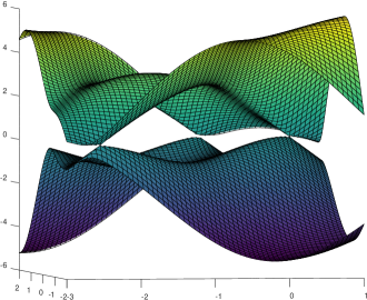
Figure 1. Eigenvalue surfaces corresponding to $A(x,y)$ from (1). There are three conical point; the surfaces appear not to touch at the middle point due to insufficient grid precision.

The problem of locating the points of eigenvalue multiplicity is of practical importance. In condensed matter physics [2] the wave propagation through periodic medium is studied via Floquet–Bloch transform [19, 20] which results in a parametric family of self-adjoint operators (or matrices) with discrete spectrum. The eigenvalue surfaces (sheets of the “dispersion relation”) may touch, see Fig. 1, which has profound effect on wave propagation and its sensitivity to a small perturbation of the medium. This touching corresponds precisely to a multiplicity in the eigenvalue spectrum. To give a well-studied example, the unusual electron properties of graphene occur due to the presence of eigenvalue multiplicity [6, 23]. It is also of practical relevance to be able to distinguish touching from “almost touching” (also known as “avoided crossing” in one-parameter problems).

The question of locating eigenvalue multiplicity in a family of $2\times 2$ real symmetric matrices $A$ has a straightforward solution (which also illustrates why the co-dimension is 2). The discriminant of $A\in\mathbb{R}^{2\times 2}$ can be written as a sum of two squares,

(2) $$\operatorname{disc}(A):=(\lambda_{1}-\lambda_{2})^{2}=(A_{11}-A_{22})^{2}+4A_{12}^{2}.$$

By definition, the discriminant is $0$ if and only if two eigenvalues coincide, therefore we have two conditions that must simultaneously be met for the multiplicity to occur:

(3) $$F(x,y)=\textbf{0},\qquad\mbox{where}\quad F:\mathbb{R}^{2}\to\mathbb{R}^{2},\quad\ F(x,y):=\begin{pmatrix}A_{11}(x,y)-A_{22}(x,y)\\ A_{12}(x,y)\end{pmatrix}.$$

Unfortunately, for larger matrices the discriminant quickly becomes unwieldy and cannot be used in practical computations. The discriminant can still be written as a sum of squares [17, 21, 25, 7], but the number of terms grows fast with the size of the matrix.

Thus, for an $n\times n$ real symmetric matrix $A(x,y)$ depending on two parameters $x$ and $y$ there is only one easily computable function $\lambda_{2}(x,y)-\lambda_{1}(x,y)$ whose root, in variables $x$ and $y$, we are seeking. However, to apply a standard method with quadratic convergence, such as the Newton–Raphson algorithm, one needs 2 functions for 2 variables. One can search for the minimum of the square eigenvalue difference, $\big{(}\lambda_{2}(x,y)-\lambda_{1}(x,y)\big{)}^{2}$, which is smooth. But such a search would converge equally well to a point of “avoided crossing”, a pitfall our proposed method manages to avoid, see Sections 5.3 and 5.4.

One can change the basis to make $A(x,y)$ block-diagonal, with a $2\times 2$ block corresponding to eigenvalues $\lambda_{1}$ and $\lambda_{2}$. The existence of this change in a neighborhood of the multiplicity point is assured (using Riesz projector) if $\lambda_{1,2}$ remain bounded away from the rest of the spectrum. However the new basis will depend on the parameters $(x,y)$ and is not directly accessible for numerical computations. Despite this obstacle, we will show that a “naive” approach produces equivalently good convergence: one can use a constant eigenvector basis which is recomputed at each point of the Newton–Raphson iteration. More precisely, we establish the following theorem.

Theorem 1.1.

Let $A({\mathbf{r}}):\mathbb{R}^{2}\mapsto\mathbb{R}^{n\times n}$ be a real symmetric matrix valued function which is continuously twice differentiable in each entry, with a non-degenerate conical point (defined below) between $\lambda_{1}$ and $\lambda_{2}$ at parameter point $\alpha$. For any ${\mathbf{r}}_{i}$, define ${\mathbf{r}}_{i+1}$ by

(4) $${\mathbf{r}}_{i+1}={\mathbf{r}}_{i}-\begin{pmatrix}\big{\langle}v_{1},\frac{\partial A}{\partial x}v_{1}\big{\rangle}-\big{\langle}v_{2},\frac{\partial A}{\partial x}v_{2}\big{\rangle}&\big{\langle}v_{1},\frac{\partial A}{\partial y}v_{1}\big{\rangle}-\big{\langle}v_{2},\frac{\partial A}{\partial y}v_{2}\big{\rangle}\\ 2\big{\langle}v_{1},\frac{\partial A}{\partial x}v_{2}\big{\rangle}&2\big{\langle}v_{1},\frac{\partial A}{\partial y}v_{2}\big{\rangle}\end{pmatrix}^{-1}\begin{pmatrix}\lambda_{1}-\lambda_{2}\\ 0\end{pmatrix}$$

where $\lambda_{1,2}=\lambda_{1,2}({\mathbf{r}}_{i})$ denote the eigenvalues of $A$ at the point ${\mathbf{r}}_{i}$ and $v_{1,2}=v_{1,2}({\mathbf{r}}_{i})$ denote the corresponding eigenvectors.

Then there exists an open neighborhood $\Omega\subset\mathbb{R}^{2}$ of $\alpha$ and a constant $C>0$ such that for all ${\mathbf{r}}_{i}\in\Omega$, the corresponding ${\mathbf{r}}_{i+1}$ satisfies the estimate

(5) $$|{\mathbf{r}}_{i+1}-\alpha|<C|{\mathbf{r}}_{i}-\alpha|^{2}.$$

Before we prove this theorem in Section 4, we explain in Section 2 the geometrical picture behind the iterative procedure (4) and also point out the main differences between (4) and the Newton–Raphson method in a conventional setting. We also review related literature in Section 2.1 once we introduce relevant notions. The precise definition and properties of “nondegenerate conical point” is given in Section 3. Section 5 contains some computational examples.

1.1. Notation

We let $C^{2}(\mathbb{R}^{2},\mathbb{R}^{n\times n})$ denote the set of matrix valued functions mapping $\mathbb{R}^{2}$ to $\mathbb{R}^{n\times n}$ with each element being continuously twice differentiable. The eigenvalues of the matrix function $A\in C^{2}(\mathbb{R}^{2},\mathbb{R}^{n\times n})$ are numbered in the increasing order $\lambda_{1}\leq\lambda_{2}\leq\lambda_{3}\leq\cdots\leq\lambda_{n}$ and without loss of generality we will look for ${\mathbf{r}}=(x,y)\in\mathbb{R}^{2}$ such that $\lambda_{1}({\mathbf{r}})=\lambda_{2}({\mathbf{r}})$. Naturally, all results apply equally well to any pair of consecutive eigenvalues. We remark that functions $\lambda_{k}({\mathbf{r}})$ are continuous but not necessarily smooth: the points of eigenvalue multiplicity are typically the points where the eigenvalues involved are not differentiable, see Fig. 1.

For any real symmetric matrix valued function $A$ and any point ${\mathbf{p}}\in\mathbb{R}^{2}$, we let $A^{\mathbf{p}}=V^{*}A({\mathbf{r}})V$ denote the representation of $A$ in the eigenvector basis computed at point ${\mathbf{p}}$. That is, $V$ is a fixed orthogonal matrix whose columns are the eigenvectors of $A({\mathbf{p}})$. The eigenvectors are assumed to be numbered according to the eigenvalue ordering. This means that $A^{\mathbf{p}}\in C^{2}(\mathbb{R}^{2},\mathbb{R}^{n\times n})$ is a diagonal matrix at the point ${\mathbf{p}}$ but not necessarily anywhere else.

We let

(6) $$\widetilde{A}^{\mathbf{p}}({\mathbf{r}})=\begin{pmatrix}A^{\mathbf{p}}_{11}&A^{\mathbf{p}}_{12}\\ A^{\mathbf{p}}_{21}&A^{\mathbf{p}}_{22}\end{pmatrix}:=\begin{pmatrix}\langle v_{1},A({\mathbf{r}})v_{1}\rangle&\langle v_{1},A({\mathbf{r}})v_{2}\rangle\\ \langle v_{2},A({\mathbf{r}})v_{1}\rangle&\langle v_{2},A({\mathbf{r}})v_{2}\rangle\end{pmatrix}$$

denote the submatrix of $A^{\mathbf{p}}$ corresponding to the eigenvectors of the coalescing eigenvalues. We stress again that the eigenvectors $v_{1}=v_{1}({\mathbf{p}})$ and $v_{2}=v_{2}({\mathbf{p}})$ are computed at the point ${\mathbf{p}}$ and do not vary with ${\mathbf{r}}$. By the definition of $A^{\mathbf{p}}$, we have

(7) $$\widetilde{A}^{\mathbf{p}}({\mathbf{p}})=\begin{pmatrix}\lambda_{1}({\mathbf{p}})&0\\ 0&\lambda_{2}({\mathbf{p}})\end{pmatrix}.$$

We let

(8) $$F\big{(}A^{\mathbf{p}}({\mathbf{r}})\big{)}:=\begin{pmatrix}A^{{\mathbf{p}}}_{11}({\mathbf{r}})-A^{{\mathbf{p}}}_{22}({\mathbf{r}})\\ 2A^{{\mathbf{p}}}_{12}({\mathbf{r}})\end{pmatrix}$$

denote the target function similar to (3). We stress that $F$ is a function of ${\mathbf{r}}$.

Throughout the paper $\mathrm{D}$ will denote the row vector of derivatives taken with respect to parameters ${\mathbf{r}}=(x,y)$,

$$\mathrm{D}f=\left(\frac{\partial f}{\partial x},\ \frac{\partial f}{\partial y}\right).$$

If $f$ is a vector-function, $\mathrm{D}f$ is a matrix with 2 columns. We use the notation $\mathrm{D}_{{\mathbf{r}}_{0}}f$ to denote the derivative evaluated at the point ${\mathbf{r}}={\mathbf{r}}_{0}$, i.e.

$$\mathrm{D}_{{\mathbf{r}}_{0}}f=\left(\frac{\partial f}{\partial x}({\mathbf{r}}_{0}),\ \frac{\partial f}{\partial y}({\mathbf{r}}_{0})\right).$$

We use notation $J_{{\mathbf{r}}}(A^{{\mathbf{p}}})$ to denote the Jacobian of $F(A^{\mathbf{p}})$,

(9) $$J_{{\mathbf{r}}}(A^{{\mathbf{p}}}):=\mathrm{D}_{{\mathbf{r}}}F(A^{\mathbf{p}})=\begin{pmatrix}\big{\langle}v_{1},\frac{\partial A}{\partial x}v_{1}\big{\rangle}-\big{\langle}v_{2},\frac{\partial A}{\partial x}v_{2}\big{\rangle}&\big{\langle}v_{1},\frac{\partial A}{\partial y}v_{1}\big{\rangle}-\big{\langle}v_{2},\frac{\partial A}{\partial y}v_{2}\big{\rangle}\\ 2\big{\langle}v_{1},\frac{\partial A}{\partial x}v_{2}\big{\rangle}&2\big{\langle}v_{1},\frac{\partial A}{\partial y}v_{2}\big{\rangle}\end{pmatrix},$$

where $v_{1},v_{2}$ are the eigenvectors of $A({\mathbf{p}})$ and the derivatives $\frac{\partial A}{\partial x}$ and $\frac{\partial A}{\partial y}$ have been evaluated at point ${\mathbf{r}}$. This is the matrix appearing in Theorem 1.1. The factor $2$ in the definition of $J_{{\mathbf{r}}}(A^{{\mathbf{p}}})$ arises naturally in calculations; it can also be used to put the second row terms in the more symmetric form,

$$2\Big{\langle}v_{1},\frac{\partial A}{\partial x}v_{2}\Big{\rangle}=\Big{\langle}v_{1},\frac{\partial A}{\partial x}v_{2}\Big{\rangle}+\Big{\langle}v_{2},\frac{\partial A}{\partial x}v_{1}\Big{\rangle}.$$

Finally, we remark that by our definitions $F(A)=F\big{(}\widetilde{A}\big{)}$ and $J_{\mathbf{r}}(A)=J_{\mathbf{r}}\big{(}\widetilde{A}\big{)}$. Therefore, the tilde (defined in equation (6)) will usually be omitted once we invoke functions $F$ and $J$.

2. Discussion

2.1. Geometric interpretation

What is described in this paper is a variation of the Newton-Raphson method searching for a zero of the objective function $\lambda_{1}({\mathbf{r}})-\lambda_{2}({\mathbf{r}})$. This is only one condition on two parameters (in the real symmetric case), and leads to an underdetermined Newton-Raphson iteration. In particular, given an initial guess ${\mathbf{r}}_{0}$, we would like to update our guess to ${\mathbf{r}}_{1}$ such that

(10) $$\mathrm{D}_{{\mathbf{r}}_{0}}\big{(}\lambda_{1}({\mathbf{r}})-\lambda_{2}({\mathbf{r}})\big{)}\,({\mathbf{r}}_{1}-{\mathbf{r}}_{0})=-\big{(}\lambda_{1}({\mathbf{r}}_{0})-\lambda_{2}({\mathbf{r}}_{0})\big{)}.$$

However, there is a whole line of points ${\mathbf{r}}_{1}$ that satisfy this condition, as illustrated in Figure 2.

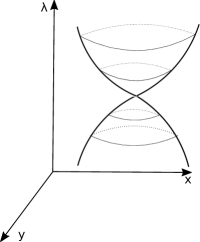
(a)

(b)

(c)

(d)

Figure 2. (a) Conical degeneracy of eigenvalues. (b) Linear approximation of top eigenvalue about the initial guess. (c) Linear approximation of bottom eigenvalue about the initial guess. (d) The intersection of the two linear approximations is a line, not a point. We need to use the conical nature of the intersection to determine a unique point to chose as our next guess.

To incorporate our knowledge that the degeneracy occurs at an isolated point, we use a heuristic derived from Berry phase [14, 4, 27], a phenomenon which underlies the inability to find a smooth diagonalization around a degeneracy: on a loop in the parameter space around a nondegenerate conical point, a continuous choice of eigenvectors must rotate by $\pi$ (as opposed to 0 mod $2\pi$).

But if smoothly going in a loop around the degeneracy rotates the eigenvectors, the direction of minimal rotation is a direction towards the point of degeneracy. Let $\{v_{1}({\mathbf{r}}),v_{2}({\mathbf{r}})\}$ be a smooth choice of normalized eigenvectors around the point ${\mathbf{r}}_{0}$ (this is possible because ${\mathbf{r}}_{0}$ is not a point of eigenvalue multiplicity). Then we are looking for the direction in the parameter space in which the eigenvector $v_{1}$ as a function of ${\mathbf{r}}$ does not rotate in the plane spanned by $\{v_{1}({\mathbf{r}}_{0}),v_{2}({\mathbf{r}}_{0})\}$ (it may still rotate “out of the plane”). This condition can be written as

(11) $$\mathrm{D}_{{\mathbf{r}}_{0}}\big{\langle}v_{1}({\mathbf{r}}),v_{2}({\mathbf{r}}_{0})\big{\rangle}\,({\mathbf{r}}_{1}-{\mathbf{r}}_{0})=0.$$

Conditions (10) and (11) together generically define a unique point ${\mathbf{r}}$ which can be taken as the next step in the iteration. We can solve for it explicitly using the well-known perturbation formulas [5, 18],

(12) $$\mathrm{D}_{{\mathbf{r}}_{0}}\lambda_{1}=\mathrm{D}_{{\mathbf{r}}_{0}}A^{{\mathbf{r}}_{0}}_{11},\qquad\mathrm{D}_{{\mathbf{r}}_{0}}\lambda_{2}=\mathrm{D}_{{\mathbf{r}}_{0}}A^{{\mathbf{r}}_{0}}_{22},$$

(13) $$\mathrm{D}_{{\mathbf{r}}_{0}}\big{\langle}v_{1}({\mathbf{r}}),v_{2}({\mathbf{r}}_{0})\big{\rangle}=\frac{\mathrm{D}_{{\mathbf{r}}_{0}}A^{{\mathbf{r}}_{0}}_{12}}{\lambda_{1}-\lambda_{2}},$$

where

(14) $$A^{{\mathbf{r}}_{0}}_{ij}=A^{{\mathbf{r}}_{0}}_{ij}({\mathbf{r}})=\big{\langle}v_{i}({\mathbf{r}}_{0}),A^{{\mathbf{r}}_{0}}({\mathbf{r}})v_{j}({\mathbf{r}}_{0})\big{\rangle}.$$

We stress that in equation (14) the eigenvectors $v_{1},v_{2}$ are evaluated at the point ${\mathbf{r}}_{0}$ and do not depend on ${\mathbf{r}}$.

The tangent planes condition (10) and the non-rotation condition (11) can now be written succinctly as

(15) $$\left[\mathrm{D}_{{\mathbf{r}}_{0}}\begin{pmatrix}A^{{\mathbf{r}}_{0}}_{11}-A^{{\mathbf{r}}_{0}}_{22}\\ 2A^{{\mathbf{r}}_{0}}_{12}\end{pmatrix}\right]({\mathbf{r}}_{1}-{\mathbf{r}}_{0})=\left[\mathrm{D}_{{\mathbf{r}}_{0}}F\big{(}A^{{\mathbf{r}}_{0}}({\mathbf{r}})\big{)}\right]({\mathbf{r}}_{1}-{\mathbf{r}}_{0})=\begin{pmatrix}\lambda_{2}-\lambda_{1}\\ 0\end{pmatrix},$$

or, less succinctly, as

$$\begin{pmatrix}\big{\langle}v_{1},\frac{\partial A}{\partial x}v_{1}\big{\rangle}-\big{\langle}v_{2},\frac{\partial A}{\partial x}v_{2}\big{\rangle}&\big{\langle}v_{1},\frac{\partial A}{\partial y}v_{1}\big{\rangle}-\big{\langle}v_{2},\frac{\partial A}{\partial y}v_{2}\big{\rangle}\\ 2\big{\langle}v_{1},\frac{\partial A}{\partial x}v_{2}\big{\rangle}&2\big{\langle}v_{1},\frac{\partial A}{\partial y}v_{2}\big{\rangle}\end{pmatrix}({\mathbf{r}}_{1}-{\mathbf{r}}_{0})=\begin{pmatrix}\lambda_{2}-\lambda_{1}\\ 0\end{pmatrix},$$

which immediately leads to (4).

Berry phase also lies at the heart of another set of works devoted to locating points of eigenvalue multiplicity. Pugliese, Dieci and co-authors [26, 9, 10, 11, 8] developed a procedure which uses Berry phase to grid-search available space and identify regions with conical points. For the final convergence they used the standard Newton–Raphson method to locate the critical point of $(\lambda_{2}-\lambda_{1})^{2}$. The convergence rate of this final step is quadratic, as in Theorem 1.1; we refer to Section 5.4 for a comparison of actual convergence in an example.

In terms of ease of application, coding equation (4) is straightforward and lack of convergence of the method also carries information (see Section 5.3 and 5.4). To perform a thorough search of all available space and to locate all conical points, it is preferable to use the methods of [26, 11, 8].

2.2. Relation to Newton-Raphson method

Recalling the definition of $\widetilde{A}^{{\mathbf{r}}_{0}}$ and in particular equation (7), we have

$$\begin{pmatrix}\lambda_{2}-\lambda_{1}\\ 0\end{pmatrix}=-F\big{(}A^{{\mathbf{r}}_{0}}({\mathbf{r}}_{0})\big{)}.$$

This allows us to rewrite equation  (15) as

$$\left[\mathrm{D}_{{\mathbf{r}}_{0}}F\big{(}A^{{\mathbf{r}}_{0}}({\mathbf{r}})\big{)}\right]\,({\mathbf{r}}_{1}-{\mathbf{r}}_{0})=-F\big{(}A^{{\mathbf{r}}_{0}}({\mathbf{r}}_{0})\big{)},$$

which is the same as a single step of Newton–Raphson iteration applied to $F(\widetilde{A}^{{\mathbf{r}}_{0}})$. In other words, ${\mathbf{r}}_{1}=(x_{1},y_{1})$ is chosen to be a solution to

(16) $$\widetilde{A}^{{\mathbf{r}}_{0}}({\mathbf{r}}_{0})+(x_{1}-x_{0})\frac{\partial\widetilde{A}^{{\mathbf{r}}_{0}}}{\partial x}({\mathbf{r}}_{0})+(y_{1}-y_{0})\frac{\partial\widetilde{A}^{{\mathbf{r}}_{0}}}{\partial y}({\mathbf{r}}_{0})=\lambda I_{2}$$

for some $\lambda\in\mathbb{R}$. Equivalently, ${\mathbf{r}}_{1}$ is the point where the linear approximation to $\widetilde{A}^{{\mathbf{r}}_{0}}({\mathbf{r}})$ has a double eigenvalue.

To understand the difference of our algorithm from a seemingly conventional Newton–Raphson method, we need to revisit the computation of $\widetilde{A}$. It can be viewed as first expressing $A({\mathbf{r}})$ in the eigenvector basis computed at the point ${\mathbf{r}}_{0}$ and then extracting the $\{1,2\}$-sub-block of the resulting matrix.

In this notation, the problem of finding the degeneracy is equivalent to finding a point ${\mathbf{r}}^{\prime}$ such that

(17) $$\widetilde{A}^{{\mathbf{r}}^{\prime}}({\mathbf{r}}^{\prime})=\lambda I_{2},\qquad\mbox{for some }\lambda\in\mathbb{R}.$$

In contrast, solving equation (16) is a first step in finding a point ${\mathbf{r}}^{\prime}$ such that

(18) $$\widetilde{A}^{{\mathbf{r}}_{0}}({\mathbf{r}}^{\prime})=\lambda I_{2},\qquad\mbox{for some }\lambda\in\mathbb{R}.$$

Going all the way to find the solution ${\mathbf{r}}^{\prime}$ to equation (18) is pointless; this is not the equation we need to solve. Instead, we go one step, computing the first Newton–Raphson approximation ${\mathbf{r}}_{1}$, and then update our target equation to

$$\widetilde{A}^{{\mathbf{r}}_{1}}({\mathbf{r}}^{\prime})=\lambda I_{2},\qquad\mbox{for some }\lambda\in\mathbb{R},$$

compute the first Newton–Raphson approximation ${\mathbf{r}}_{2}$ to that equation and so on.

2.3. Complex Hermitian matrices

Let us now consider a complex Hermitian matrix-valued function $A\in C^{2}(\mathbb{R}^{3},\mathbb{C}^{n\times n})$. To find a point of eigenvalue multiplicity, we typically need three real parameters (the off diagonal terms can be complex, and that introduces an additional degree of freedom), which we still denote by ${\mathbf{r}}=(x,y,z)$.

The conditions can now be written as

(19) $$\left[\mathrm{D}_{{\mathbf{r}}_{0}}G\big{(}A^{{\mathbf{r}}_{0}}({\mathbf{r}})\big{)}\right]({\mathbf{r}}_{1}-{\mathbf{r}}_{0})=\begin{pmatrix}\lambda_{2}-\lambda_{1}\\ 0\\ 0\end{pmatrix},$$

where

(20) $$G\big{(}A^{{\mathbf{r}}_{0}}\big{)}=\begin{pmatrix}A^{{\mathbf{r}}_{0}}_{11}-A^{{\mathbf{r}}_{0}}_{22}\\ 2A^{{\mathbf{r}}_{0}}_{12}\\ 2A^{{\mathbf{r}}_{0}}_{21}\end{pmatrix}.$$

One can equivalently use the objective function

(21) $$G\big{(}A^{{\mathbf{r}}_{0}}\big{)}=\begin{pmatrix}A^{{\mathbf{r}}_{0}}_{11}-A^{{\mathbf{r}}_{0}}_{22}\\ 2\operatorname{Re}(A^{{\mathbf{r}}_{0}}_{12})\\ 2\operatorname{Im}(A^{{\mathbf{r}}_{0}}_{21})\end{pmatrix}.$$

3. Conical Intersection

Let $\alpha$ be a point in the parameter space such that $A(\alpha)$ has a double eigenvalue $\lambda_{1}=\lambda_{2}$. The existence of eigenvalue multiplicity precludes a smooth diagonalization in a region containing the degeneracy. However, a smooth block diagonalization exists. The standard construction (see, for example, [18, II.4.2 and Remark 4.4 therein]) uses Riesz projector.

We can choose a contour $\gamma:[0,1]\mapsto\mathbb{C}$ with $\gamma(0)=\gamma(1)$ enclosing $\lambda_{1}$, $\lambda_{2}$ and no other point in the spectrum of $A(\alpha)$. This property of $\gamma$ must persist for $A({\mathbf{r}})$ when ${\mathbf{r}}$ is in a small neighborhood of $\alpha$. The Riesz projector

(22) $$P({\mathbf{r}})=\int_{\gamma}(A({\mathbf{r}})-\lambda I_{n})^{-1}d\lambda$$

projects onto the space spanned by the eigenvectors of $\lambda_{1}({\mathbf{r}})$ and $\lambda_{2}({\mathbf{r}})$ [15]. The projector itself is smooth, as the points on the contour are all in the resolvent set of $A$ (and so $A-\lambda I_{n}$ has a bounded inverse for all $\lambda\in\Gamma$). Starting with an arbitrary eigenvector basis $\{v_{1},v_{2}\}$ at $\alpha$, we can obtain a basis at a nearby ${\mathbf{r}}$ by applying Gram-Schmidt procedure to the set $\left\{P({\mathbf{r}})v_{1},P({\mathbf{r}})v_{2}\right\}$, which preserves smoothness. We can do the same with the orthogonal complement $I-P({\mathbf{r}})$ and a complementary basis to $\{v_{1},v_{2}\}$. To summarize, for some region $\Omega\in\mathbb{R}^{2}$ with $\alpha\in\Omega$, we find a change of basis $M(\cdot)\in C^{2}(\Omega,R^{n\times n})$ such that

(23) $$M({\mathbf{r}})^{*}A({\mathbf{r}})M({\mathbf{r}})=B({\mathbf{r}})\oplus\Lambda({\mathbf{r}}),$$

where $B\in C^{2}(\Omega,\mathbb{R}^{2\times 2})$ and $\Lambda\in C^{2}(\Omega,\mathbb{R}^{(n-2)\times(n-2)})$. We can further diagonalize both $B$ and $A$ at any point ${\mathbf{r}}_{0}$ to obtain

(24) $$\Gamma({\mathbf{r}})^{*}A^{{\mathbf{r}}_{0}}({\mathbf{r}})\Gamma({\mathbf{r}})=B^{{\mathbf{r}}_{0}}({\mathbf{r}})\oplus\Lambda({\mathbf{r}}),$$

where $\Gamma({\mathbf{r}})=V^{T}M({\mathbf{r}})(W\oplus I_{n-2})\in C^{2}(\Omega,R^{n\times n})$, and both

$$A^{{\mathbf{r}}_{0}}(\cdot):=V^{T}A(\cdot)V\qquad\mbox{and}\qquad B^{{\mathbf{r}}_{0}}(\cdot):=W^{T}B(\cdot)W$$

are diagonal at ${\mathbf{r}}_{0}$. A stronger result from Hsieh, and Sibuya [16], and Gingold [13] states that such block-diagonalization exists even for matrices that are not necessarily Hermitian, and for any closed rectangular region that contains an isolated degeneracy.

Note that since $B$ is a $2\times 2$ matrix which has an eigenvalue multiplicity at the point $\alpha$, $B(\alpha)$ is a multiple of the identity. The eigenvalue multiplicity is detected by the discriminant of $B$ which in the $2\times 2$ case is defined as

(25) $$\operatorname{disc}(B):=(\lambda_{1}-\lambda_{2})^{2}=(B_{11}-B_{22})^{2}+4B_{12}^{2}.$$

The discriminant achieves its minimum value 0 at the point $\alpha$. It is also a $C^{2}$ function of ${\mathbf{r}}$ and its Hessian is well-defined.

Definition 3.1.

A point of eigenvalue multiplicity $\alpha$ is a non-degenerate conical point if $\operatorname{disc}(B({\mathbf{r}}))$ has a non-degenerate critical point at ${\mathbf{r}}=\alpha$.

In other words, there is a positive definite matrix $H$ (the “Hessian”) such that

$$\operatorname{disc}(B({\mathbf{r}}))=\big{\langle}({\mathbf{r}}-\alpha),H({\mathbf{r}}-\alpha)\big{\rangle}+o\!\left(|{\mathbf{r}}-\alpha|^{2}\right),$$

and therefore, along any ray originating at $\alpha$, the eigenvalues are separating at a non-zero linear rate. This picture justifies the use of the term “conical”.

Unfortunately, while existence of $B({\mathbf{r}})$ is assured, it is not easily accessible. The following theorem provides a more practical method of checking if $\alpha$ is non-degenerate.

Theorem 3.2.

The Hessian of $\operatorname{disc}(B)$ at $\alpha$ is given by

(26) $$\operatorname{Hess}_{\alpha}(\operatorname{disc}(B))=2J_{\alpha}(B)^{T}J_{\alpha}(B)=2J_{\alpha}(A^{\alpha})^{T}J_{\alpha}(A^{\alpha}).$$

Consequently, $\alpha$ is a non-degenerate conical point if and only if $\det J_{\alpha}(A^{\alpha})\neq 0$.

The condition $\det J_{\alpha}(A^{\alpha})\neq 0$ has a nice geometric meaning: it is precisely the condition that the manifold $\widetilde{A}^{\alpha}$ of $2\times 2$ real symmetric matrices is transversal to the line of $2\times 2$ symmetric matrices with repeated eigenvalues (cf. [24, Def. 1]).

The choice of basis in the definition of $\widetilde{A}^{\alpha}$ is assumed to align with the choice of basis used to compute $B({\mathbf{r}})$, i.e. the first two columns of $M(\alpha)$ are the eigenvectors used to compute $\widetilde{A}^{\alpha}$. This choice does not affect the definition of the non-degenerate point because of the following lemma.

Lemma 3.3.

Let $A\in C^{2}(\mathbb{R}^{2},\mathbb{R}^{2\times 2})$ be a $2\times 2$ matrix-valued function of ${\mathbf{r}}\in\mathbb{R}^{2}$. Then for any orthogonal matrix $U\in\mathbb{R}^{2\times 2}$ there is an orthogonal matrix $W\in\mathbb{R}^{2\times 2}$ such that for all ${\mathbf{r}}$ we have

(27) $$F(U^{T}AU)=WF(A),\qquad J_{\mathbf{r}}(U^{T}AU)=WJ_{\mathbf{r}}(A),$$

and therefore

(28) $$\left|\det(J_{\mathbf{r}}(A))\right|=\left|\det(J_{\mathbf{r}}(U^{T}AU))\right|.$$

Proof.

This identity for $2\times 2$ matrix-functions can be checked by direct computation but the details are excessively tedious. Instead we use a more generalizable approach.

We fix an orthogonal $U$ and let $\mathcal{S}^{2}$ denote the linear space of $2\times 2$ real symmetric matrices. The map $F$, see equation (8), acts as a linear transformation from $\mathcal{S}^{2}$ to $\mathbb{R}^{2}$. It is obviously onto and has the kernel $\operatorname{Ker}(F)$ consisting of multiples of the identity. On the other hand, conjugation by $U$ (namely the map $A\mapsto U^{T}AU$) is a linear transformation of $\mathcal{S}^{2}$ to itself. It maps multiples of the identity to themselves and therefore induces a linear transformation from the quotient space $\mathcal{S}^{2}/\operatorname{Ker}(F)$ to itself. This linear transformation, via the isomorphism $F$ between $\mathcal{S}^{2}/\operatorname{Ker}(F)$ and $\mathbb{R}^{2}$, induces a linear transformation on $\mathbb{R}^{2}$ mapping $F(A)$ to $F(U^{T}AU)$.

We summarize the above in the commutative diagram

$$\begin{CD}\mathcal{S}^{2}@>{A\mapsto U^{T}AU}>{}>\mathcal{S}^{2}\\ @V{F}V{}V@V{F}V{}V\\ \mathbb{R}^{2}@>{W}>{}>\mathbb{R}^{2}\end{CD}$$

In other words, for a given orthogonal $U$, there exists a constant $2\times 2$ matrix $W$ such that

$$F(U^{T}AU)=WF(A).$$

From the identity (see (25) for the definition of discriminant)

$$\left|F(A)\right|^{2}=\operatorname{disc}(A)=\operatorname{disc}(U^{T}AU)=\left|F(U^{T}AU)\right|^{2}$$

we conclude that $W$ is orthogonal. Finally, taking derivatives we get

$$J(U^{T}AU)=WJ(A),\quad\implies\quad\det(J(U^{T}AU))=\det(WJ(A))=\pm\det(J(A)),$$

since determinant of an orthogonal matrix is either $1$ or $-1$. ∎

The following identity will be helpful in the proof of Theorem 3.2 and also in Section 4.

Lemma 3.4.

For any $A^{{\mathbf{r}}_{0}}$ and $B^{{\mathbf{r}}_{0}}$ as in equation (24),

(29) $$J_{{\mathbf{r}}_{0}}(B^{{\mathbf{r}}_{0}})=J_{{\mathbf{r}}_{0}}(A^{{\mathbf{r}}_{0}})+2(\lambda_{2}-\lambda_{1})\begin{pmatrix}0&0\\ \big{\langle}\frac{\partial\gamma_{1}}{\partial x},\gamma_{2}\big{\rangle}&\big{\langle}\frac{\partial\gamma_{1}}{\partial y},\gamma_{2}\big{\rangle}\end{pmatrix},$$

where $\gamma_{1,2}=\gamma_{1,2}({\mathbf{r}}_{0})$ are the first two columns of the matrix $\Gamma({\mathbf{r}}_{0})$.

Proof.

We remark that identity (29) is only claimed for the Jacobian evaluated at the point where both $A^{{\mathbf{r}}_{0}}$ and $B^{{\mathbf{r}}_{0}}$ are diagonal, therefore $A^{{\mathbf{r}}_{0}}\gamma_{j}({\mathbf{r}}_{0})=\lambda_{j}({\mathbf{r}}_{0})\gamma_{j}({\mathbf{r}}_{0})$.

For all ${\mathbf{r}}$, $\gamma_{j}({\mathbf{r}})$ are orthonormal and differentiating $\langle\gamma_{i},\gamma_{j}\rangle=\mathrm{const}$ we get

(30) $$\left\langle\frac{\partial\gamma_{i}}{\partial x},\gamma_{j}\right\rangle=-\left\langle\gamma_{i},\frac{\partial\gamma_{j}}{\partial x}\right\rangle.$$

We can now relate the derivatives of $A^{{\mathbf{r}}_{0}}$ to the derivatives of $B^{{\mathbf{r}}_{0}}$,

$$\frac{\partial}{\partial x}(B^{{\mathbf{r}}_{0}}_{ij}) =\frac{\partial}{\partial x}\big{\langle}\gamma_{j},A^{{\mathbf{r}}_{0}}\gamma_{i}\big{\rangle}$$

$$=\left\langle\gamma_{i},\frac{\partial A^{{\mathbf{r}}_{0}}}{\partial x}\gamma_{j}\right\rangle+\left\langle\frac{\partial\gamma_{i}}{\partial x},A^{{\mathbf{r}}_{0}}\gamma_{j}\right\rangle+\left\langle\gamma_{i},A^{{\mathbf{r}}_{0}}\frac{\partial\gamma_{j}}{\partial x}\right\rangle$$

$$=\frac{\partial A^{{\mathbf{r}}_{0}}_{ij}}{\partial x}+\lambda_{j}\left\langle\frac{\partial\gamma_{i}}{\partial x},\gamma_{j}\right\rangle+\lambda_{i}\left\langle\gamma_{i},\frac{\partial\gamma_{j}}{\partial x}\right\rangle$$

$$=\frac{\partial A^{{\mathbf{r}}_{0}}_{ij}}{\partial x}+(\lambda_{j}-\lambda_{i})\left\langle\frac{\partial\gamma_{i}}{\partial x},\gamma_{j}\right\rangle,\qquad i,j\in\{1,2\}.$$

The calculation is identical for $y$ derivatives. ∎

Proof of Theorem 3.2.

We write

$$\operatorname{disc}(B)=(B_{11}-B_{22})^{2}+4B_{12}^{2}=\left\langle F(B),F(B)\right\rangle,$$

and note that $F(B(\alpha))=\mathbf{0}$. The latter observation implies that the product rule for the second derivatives at the point $\alpha$ collapses to

$$\frac{\partial^{2}}{\partial x_{i}\partial x_{j}}\left\langle F(B),F(B)\right\rangle=2\left\langle\frac{\partial F(B)}{\partial x_{i}},\frac{\partial F(B)}{\partial x_{j}}\right\rangle,\qquad x_{i},x_{j}\in\{x,y\}.$$

Therefore the Hessian can be written as

$$\operatorname{Hess}_{\alpha}\langle F(B),F(B)\rangle=2\begin{pmatrix}\frac{\partial F(B)^{T}}{\partial x}\\[5.0pt] \frac{\partial F(B)^{T}}{\partial y}\end{pmatrix}\begin{bmatrix}\frac{\partial F(B)}{\partial x}&\frac{\partial F(B)}{\partial y}\end{bmatrix}=2J_{\alpha}(B)^{T}J_{\alpha}(B).$$

Finally, setting ${\mathbf{r}}_{0}=\alpha$ in Lemma 3.4 yields

(31) $$J_{\alpha}(B)=J_{\alpha}(A^{\alpha}),$$

and concludes the proof of (26). ∎

4. Proof of the main result

Here we restate the procedure used to locate the degeneracy in the notation that has been introduced.

Theorem 4.1.

Let $\sigma\colon C^{2}(\mathbb{R}^{2},\mathbb{R}^{2\times 2})\times\mathbb{R}^{2}\to\mathbb{R}^{2}$ be defined by

(32) $$\sigma(S,{\mathbf{r}})={\mathbf{r}}-J_{{\mathbf{r}}}(S)^{-1}F_{\mathbf{r}}(S).$$

Let $A\in C^{2}(\mathbb{R}^{2},\mathbb{R}^{n\times n})$ have a non-degenerate conical point at $\alpha$ between eigenvalues $\lambda_{1}$ and $\lambda_{2}$. Then there exists an open $\Omega\subset\mathbb{R}^{2}$ with $\alpha\in\Omega$ and $\exists C\in\mathbb{R}$, such that for all ${\mathbf{r}}\in\Omega$,

(33) $$|\sigma(\widetilde{A}^{{\mathbf{r}}},{\mathbf{r}})-\alpha|<C|{\mathbf{r}}-\alpha|^{2},$$

where the $2\times 2$ matrix-function $\widetilde{A}^{{\mathbf{r}}}(\cdot)\in C^{2}(\mathbb{R}^{2},\mathbb{R}^{2\times 2})$ is defined by

(34) $$\widetilde{A}^{{\mathbf{r}}}(\cdot)=V^{T}A(\cdot)V,$$

with the constant $n\times 2$ matrix $V=(v_{1}\ v_{2})$ whose columns are the eigenvectors of $A({\mathbf{r}})$.

We remark that non-degeneracy of the conical point is a generic property: any degenerate conical point can be made non-degenerate by a small perturbation of the function $A$.

We recall that the superscript in $\widetilde{A}^{{\mathbf{r}}}(\cdot)$ refers to the basis which is computed at the point ${\mathbf{r}}$ and in which the matrix $A(x,y)$ is represented. The derivatives of $\widetilde{A}^{{\mathbf{r}}}(\cdot)$ that are taken to compute $J_{\mathbf{r}}$ in (32), are also evaluated at the point ${\mathbf{r}}$. The result of evaluating $\sigma(\widetilde{A}^{{\mathbf{r}}},{\mathbf{r}})$ is explicitly written out in equation (4).

Proof.

Let $B$ be the matrix defined in equation (23). We will see, in Lemmas 4.2 and 4.4 below, that there is a neighborhood $\Omega\subset\mathbb{R}^{2}$ of the conical point $\alpha$, and constants $C_{1},C_{2}>0$ such that for all ${\mathbf{r}}\in\Omega$ we have

$$|\sigma(B,{\mathbf{r}})-\alpha|<C_{1}|{\mathbf{r}}-\alpha|^{2}$$

and

$$|\sigma(B,{\mathbf{r}})-\sigma(\widetilde{A}^{{\mathbf{r}}},{\mathbf{r}})|<C_{2}|{\mathbf{r}}-\alpha|^{2}.$$

Together, these give us

$$|\sigma(\widetilde{A}^{{\mathbf{r}}},{\mathbf{r}})-\alpha|<(C_{1}+C_{2})|{\mathbf{r}}-\alpha|^{2},$$

as desired. ∎

Now we establish the lemmas used in the proof of Theorem 4.1.

Lemma 4.2.

There exists $\Omega_{1}\subset\mathbb{R}^{2}$ with $\alpha\in\Omega_{1}$ and $C_{1}\in\mathbb{R}$ such that

(35) $$|\sigma(B,{\mathbf{r}})-\alpha|<C_{1}|{\mathbf{r}}-\alpha|^{2},$$

when ${\mathbf{r}}\in\Omega_{1}$.

Proof.

This is the usual Newton–Raphson method applied to conical point search for the $2\times 2$ matrix $B$. For completeness we provide the proof. For the function $F({\mathbf{r}}):=F(B({\mathbf{r}}))$, we have the Taylor expansion around the point ${\mathbf{r}}_{0}$ which is evaluated at the point $\alpha$,

$$\textbf{0}=F(\alpha)=F({\mathbf{r}}_{0})+\mathrm{D}_{{\mathbf{r}}_{0}}F\cdot(\alpha-{\mathbf{r}}_{0})+O(|\alpha-{\mathbf{r}}_{0}|^{2}),$$

where the constant in $O(|\alpha-{\mathbf{r}}_{0}|^{2})$ is independent of ${\mathbf{r}}_{0}$ as long as it is in a neighborhood $\widetilde{\Omega}_{1}$ of $\alpha$. The dot denotes the matrix-by-vector multiplication (to distinguish it from the argument of the function $F$).

By assumption $\det(J_{\alpha})\neq 0$, and, by smoothness, we know that $\mathrm{D}_{{\mathbf{r}}_{0}}F=J_{{\mathbf{r}}_{0}}$ is boundedly invertible in some region $\Omega_{1}\subset\widetilde{\Omega}_{1}$ containing $\alpha$. Therefore, for the point ${\mathbf{r}}_{1}=\sigma(B,{\mathbf{r}}_{0})$, or equivalently,

$$J_{{\mathbf{r}}_{0}}\cdot({\mathbf{r}}_{1}-{\mathbf{r}}_{0})=-F({\mathbf{r}}_{0}),$$

we have

$$\textbf{0}=J_{{\mathbf{r}}_{0}}\cdot(\alpha-{\mathbf{r}}_{1})+O(|\alpha-{\mathbf{r}}_{0}|^{2}),$$

with the estimate (35) following by inverting $J_{{\mathbf{r}}_{0}}$. ∎

Lemma 4.3.

For any $B\in C^{2}(\mathbb{R}^{2},\mathbb{R}^{n\times n})$ and constant, orthogonal $U$, we have

(36) $$\sigma(B,{\mathbf{r}})=\sigma(U^{T}BU,{\mathbf{r}}).$$

Proof.

Equation (36) follows directly from the definition of the one-step iteration function $\sigma$ and Lemma 3.3. ∎

Lemma 4.4.

There exists $\Omega_{2}\subset\mathbb{R}^{2}$ with $\alpha\in\Omega_{2}$ and $C_{2}\in\mathbb{R}$ such that

(37) $$|\sigma(B,{\mathbf{r}})-\sigma(\widetilde{A}^{{\mathbf{r}}},{\mathbf{r}})|<C_{2}|{\mathbf{r}}-\alpha|^{2},$$

when ${\mathbf{r}}\in\Omega_{2}$.

Proof.

By the assumption that $\alpha$ is a non-degenerate conical point and equation (26), we have that $J_{\mathbf{r}}(B)$ and therefore $J_{\mathbf{r}}(B^{{\mathbf{r}}})$ has a bounded inverse in a region around $\alpha$. By equation (29) we conclude that $J_{\mathbf{r}}(\widetilde{A}^{{\mathbf{r}}})$ also has a bounded inverse in some region $\Omega_{2}$ around $\alpha$ where $\lambda_{1}-\lambda_{2}$ is small. We can express the difference of the inverses as

$$J_{\mathbf{r}}(B^{{\mathbf{r}}})^{-1}-J_{\mathbf{r}}(\widetilde{A}^{{\mathbf{r}}})^{-1} =J_{\mathbf{r}}(B^{{\mathbf{r}}})^{-1}\left(J_{\mathbf{r}}(\widetilde{A}^{{\mathbf{r}}})-J_{\mathbf{r}}(B^{{\mathbf{r}}})\right)J_{\mathbf{r}}(\widetilde{A}^{{\mathbf{r}}})^{-1}$$

$$=(\lambda_{1}-\lambda_{2})J_{\mathbf{r}}(B^{{\mathbf{r}}})^{-1}\begin{pmatrix}0&0\\ \big{\langle}\frac{\partial\gamma_{1}}{\partial x},\gamma_{2}\big{\rangle}&\big{\langle}\frac{\partial\gamma_{1}}{\partial y},\gamma_{2}\big{\rangle}\end{pmatrix}J_{\mathbf{r}}(\widetilde{A}^{{\mathbf{r}}})^{-1}.$$

and so, using boundedness of $\Gamma$ and its derivatives, we get

$$\left\|J_{\mathbf{r}}(B^{{\mathbf{r}}})^{-1}-J_{\mathbf{r}}(\widetilde{A}^{{\mathbf{r}}})^{-1}\right\|=O(\lambda_{1}-\lambda_{2}).$$

We also recall that by definition of $A^{\mathbf{r}}$ and $B^{\mathbf{r}}$,

$$F(B^{\mathbf{r}})=F(\widetilde{A}^{{\mathbf{r}}})=\begin{pmatrix}\lambda_{1}({\mathbf{r}})-\lambda_{2}({\mathbf{r}})\\ 0\end{pmatrix}.$$

Finally, abbreviating $J=J_{{\mathbf{r}}}$, we estimate

$$\left|\sigma(B^{{\mathbf{r}}},{\mathbf{r}})-\sigma(\widetilde{A}^{{\mathbf{r}}},{\mathbf{r}})\right| =\left|J(B^{{\mathbf{r}}})^{-1}F(B^{{\mathbf{r}}})-J(\widetilde{A}^{{\mathbf{r}}})^{-1}F(\widetilde{A}^{{\mathbf{r}}})\right|$$

$$=\left|\left(J(B^{{\mathbf{r}}})^{-1}-J(\widetilde{A}^{{\mathbf{r}}})^{-1}\right)F(\widetilde{A}^{{\mathbf{r}}})\right|$$

$$\leq\left\|J(B^{{\mathbf{r}}})^{-1}-J(\widetilde{A}^{{\mathbf{r}}})^{-1}\right\|\,\left|F(\widetilde{A}^{{\mathbf{r}}})\right|$$

$$=O\left((\lambda_{2}-\lambda_{1})^{2}\right)=O\left(|{\mathbf{r}}-\alpha|^{2}\right).$$

Equation (37) now follows by applying Lemma 4.3 to get $\sigma(B^{{\mathbf{r}}},{\mathbf{r}})=\sigma(B,{\mathbf{r}})$. ∎

5. Examples

5.1. Elements of A are linear in parameters

If $A$ is linear in each parameter, we have $A=\Lambda I+xA_{x}+yA_{y}=\Lambda I+\alpha I+\beta\sigma_{1}+\gamma\sigma_{3}$, where

$$\sigma_{1}=\begin{pmatrix}0&1\\ 1&0\end{pmatrix}\qquad\mbox{and}\qquad\sigma_{3}=\begin{pmatrix}1&0\\ 0&-1\end{pmatrix},$$

for some $\alpha$, $\beta$ that depend on $x,y$, and $A$. The eigenvalues of this matrix are values of $\lambda$ where

$$\det(A-\lambda I)=\det(\Lambda I+\alpha I+\beta\sigma_{1}+\gamma\sigma_{3}-\lambda I)=0$$

$$(\Lambda+\alpha-\lambda)^{2}=\beta^{2}+\gamma^{2}$$

$$\lambda=\Lambda+\alpha\pm\sqrt{\beta^{2}+\gamma^{2}}$$

which is a cone in the new parameter space. In fact, a simple calculation shows that the degeneracy of the function $\hat{A}(\alpha,\beta)=\begin{pmatrix}\beta&\gamma\\ \gamma&-\beta\end{pmatrix}$, which has the same eigenvectors and shifted eigenvalues, can be located using a single step of iteration (4).

5.2. Non-linear examples

Consider the following matrix-function example,

(38) $$A(x,y)=\begin{pmatrix}2\cos(x)&0&0&1\\ 0&0.5+\cos(y)&0&1\\ 0&0&1&1\\ 1&1&1&1\end{pmatrix}.$$

Since $A(x,y)$ is a rank-one perturbation of a diagonal matrix, it can be shown that there is a double eigenvalue $1$ at the point given by

$$2\cos(x)=0.5+\cos(y)=1,$$

or $x=y=\pi/3$. The results of running the algorithm of Theorem 1.1 with random starting points in the rectangle $(\frac{\pi}{3},\frac{\pi}{3})\pm\frac{1}{2}$ is shown in Figure 3a.

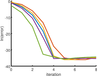
(a)

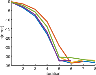
(b)

Figure 3. (A) Logarithm of the distance from the $i$-th iteration ${\mathbf{r}}_{i}$ to the conical point $(\frac{\pi}{3},\frac{\pi}{3})$ of $A(x,y)$ from equation (38), plotted as a function of $i$; the algorithm saturates at the limit of numerical precision in 3-5 steps. (B) Logarithm of $|{\mathbf{r}}_{i+1}-{\mathbf{r}}_{i}|$ where ${\mathbf{r}}_{i}$ is the $i$-th iteration of the algorithm applied to $A(x,y,z)$ given by equation (39). Several independent runs are plotted, each beginning at a random point in $[-\pi,\pi]$.

The complex Hermitian case described in Section 2.3 is demonstrated in Figure 3b. The matrix

(39) $$A=\begin{pmatrix}1&1&0&0&0&0&0&0&0&z\\ 1&3&e^{ix}&1&0&0&0&0&0&0\\ 0&e^{-ix}&2&1&0&0&0&0&0&0\\ 0&1&1&3&1&0&0&0&0&0\\ 0&0&0&1&3&1&1&0&0&0\\ 0&0&0&0&1&3&0&0&0&0\\ 0&0&0&0&1&0&3&1&1&0\\ 0&0&0&0&0&0&1&2&e^{iy}&0\\ 0&0&0&0&0&0&1&e^{-iy}&3&1\\ z&0&0&0&0&0&0&0&1&1\end{pmatrix}.$$

corresponds to the discrete Laplacian of the graph shown in Figure 4 with dashed edges carrying a magnetic potential ($x$ and $y$ correspondingly). The parameter $z$ is introduced artificially, and the conical point found numerically has value $z=0$. Since the location of the conical point is not known analytically, the error is estimated using the norms of updates $\left\|{\mathbf{r}}_{i}-{\mathbf{r}}_{i+1}\right\|$ instead of $\left\|{\mathbf{r}}_{i}-\alpha\right\|$. The result of several runs of the algorithm is shown in Figure 3b.

Figure 4. Graph corresponding to equation (39).

5.3. Avoided crossing

While a non-degenerate conical point is stable under small perturbations of the real symmetric matrix-function $A(x,y)$, the eigenvalue multiplicity may be lifted by an addition of a small complex perturbation. It is instructive to investigate the run results of our algorithm in this case.

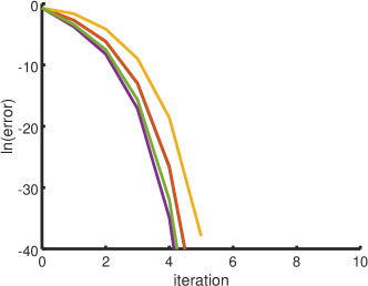
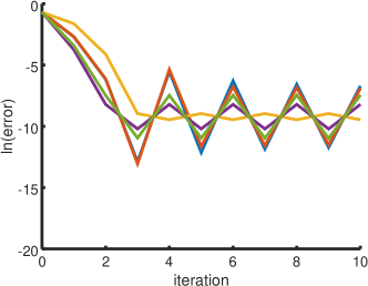
Figure 5. Logarithm of distance to $(0,0)$ as a function of the iteration step for several runs of the algorithm for $A(x,y)$ given by equation (40) with $\epsilon=0$ (left) and with $\epsilon=10^{-4}$ (right), i.e. an avoided crossing. Note the difference in vertical scales. Runs are initialized with random points on the circle of radius $1/2$ around $(0,0)$.

Consider the matrix-function

(40) $$A=\begin{pmatrix}x+3\sin(y)&y+\epsilon i\\ y-\epsilon i&-x-x^{2}\end{pmatrix}.$$

It has a conical point at $(0,0)$ when $\epsilon=0$ and no eigenvalue multiplicities when $\epsilon\neq 0$. We plot in Figure 5 the results of several runs with $\epsilon=0$ (left) and with $\epsilon=10^{-4}$ (right). For $\epsilon=0$ the algorithm converges quadratically, as in the previous examples. For $\epsilon\neq 0$, the algorithm initially approaches the position of the former conical point, but gets repelled, resulting in oscillations. Conversely, such oscillations (within the limits of numerical precision) should be considered a tell-tale sign of eigenvalue surfaces nearly but not exactly touching.

We remark that for $\epsilon\neq 0$, the square eigenvalue difference $(\lambda_{1}-\lambda_{2})^{2}$ has the minimal value of order $\epsilon^{2}$. If one is using optimization of $(\lambda_{1}-\lambda_{2})^{2}$ to find the multiplicity location, it would be difficult to tell apart genuine points of multiplicty from avoided crossings. This observation is investigated further in the next example.

5.4. Merging Dirac points

In condensed matter physics literature, the conical points in the dispersion relation of a periodic structure are know as the “Dirac points”, because the effective equation of the wave propagation at the corresponding energy is of Dirac type (see [12] for a mathematical formulation of this physics result). When the material parameters change, the Dirac point may undergo a fold bifurcation, where two points collide and annihilate. The physical consequence of this collision were studied, for example, in [22]; an experimental observation in a tunable honeycomb lattice was reported in [28]. In this section we use the basic model from [22],

(41) $$A(x,y):=\begin{pmatrix}0&-1-\frac{1}{2}e^{ix}-pe^{iy}\\ -1-\frac{1}{2}e^{-ix}-pe^{-iy}&0\end{pmatrix},$$

where the bifurcation occurs at $p=\frac{1}{2}$: for $p>\frac{1}{2}$ there are two Dirac points and for $p<\frac{1}{2}$ there are none, see Fig. 6.

Despite $A(x,y)$ being a complex matrix, the problem of locating Dirac points in this setting is analogous to the real symmetric case due to presence of the inversion symmetry $\overline{A(-x,-y)}=A(x,y)$. The correct target function $F$ (cf. (8) and (21)) is

$$F(A^{\mathbf{p}}):=\begin{pmatrix}A^{{\mathbf{p}}}_{11}-A^{{\mathbf{p}}}_{22}\\ 2\operatorname{Im}(A^{{\mathbf{p}}}_{12})\end{pmatrix}.$$

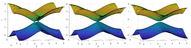
Figure 6. Two Dirac points (left), colliding (center) and disappearing (right), in the dispersion relation of (41) with parameter $p$ values $0.6$, $0.5$ and $0.45$ correspondingly.

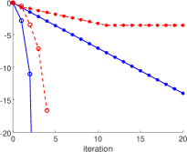
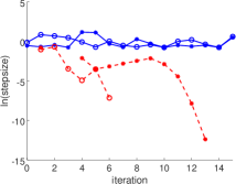
Figure 7. Convergence of iterations for matrix family (41): applying Theorem 1.1 (blue, solid) versus quasi-Newton minimization of $(\lambda_{1}-\lambda_{2})^{2}$ (red, dashed). The parameter $p$ is $0.6$ (left), $0.5$ (center) and $0.45$ (right). Two starting points used in each figure, $(0.8\pi,0.8\pi)$ (empty circles) and $(0.8\pi,1.2\pi)$ (stars).

In Figure 7 we present a comparison between the convergence of iterations of Theorem 1.1 and a standard quasi-Newton search for the minimum of $g(x,y)=(\lambda_{1}-\lambda_{2})^{2}$. Figure 7(left) is for $p=0.6$ where the convergence of both methods is quadratic, although Theorem 1.1 is faster. Figure 7(center) is for $p=0.5$, where the multiplicity point is degenerate. While Theorem 1.1 is no longer applicable, the iteration still converges when the matrix pseudoinverse is used in (4). The speed of iteration is highly dependent on the direction, presumably because the cross-section of the eigenvalue surface is parabolic in one direction and conical in the other. Again, the algorithm of Theorem 1.1 converges faster, while quasi-Newton iteration fails altogether for the second initial point.

Finally, in Figure 7(right), the $Y$-axis shows the logarithm of the last taken step, since the distance to the conical point is undefined: there is no conical point. While the quasi-Newton iteration converges, correctly, to the minimum of $(\lambda_{1}-\lambda_{2})^{2}$ located at $(\pi,\pi)$, the algorithm of Theorem 1.1 is not converging, indicating the absence of the conical point in that area.

To interpret the results, recall that a quasi-Newton minimization is searching for the zero of the gradient of $g$ using a numerical approximation of the Hessian of $g$. But according to Theorem 3.2, the matrix appearing in equation (4) is equal to the leading term of the Hessian (or its square root) around the conical point. It is therefore natural to expect a faster convergence.

To give an analogy, consider finding the root of $f(x)=x^{2}-a$ via the Newton–Raphson scheme (thus computing $f^{\prime}$ as done in Theorem 1.1) or via minimization of $g(x)=f^{2}(x)$ (thus computing $g^{\prime\prime}$ in the course of finding the root of $g^{\prime}$). Of course, close to the root, $g^{\prime\prime}\approx(f^{\prime})^{2}$, so the two schemes give equivalent rates of convergence, but having an analytical expression for $f^{\prime}$ naturally produces better results than performing a numerical approximation of $g^{\prime\prime}$.

Theorem 1.1) would thus be beneficial in any situation where computing two eigenvectors is not significantly more expensive than sampling the eigenvalues several times. One example of such circumstances is given by differential operators on metric graphs [3], where the eigenvalues are found by solving the “secular equation” of the form $\det\left(I-S(\sqrt{\lambda})\right)=0$, and, once an eigenvalue is identified, the corresponding eigenvector of $S(\sqrt{\lambda})$ gives the (Fourier coefficients of the) eigenvector on the graph. The latter operation is inexpensive relative to repeated evaluation of the determinant necessary for locating the root $\lambda$.

5.5. Locating points of higher multiplicity

We can apply a modification of the method to search for points of higher multiplicity in a family of matrices with sufficient number of parameters. For example, for locating a triple eigenvalue of a 5-parameter family $A$ we use

(42) $$F(A^{\mathbf{p}})=\begin{pmatrix}A^{\mathbf{p}}_{11}-A^{\mathbf{p}}_{22}\\ A^{\mathbf{p}}_{22}-A^{\mathbf{p}}_{33}\\ 2A^{\mathbf{p}}_{12}\\ 2A^{\mathbf{p}}_{13}\\ 2A^{\mathbf{p}}_{23}\end{pmatrix},$$

where $A^{\mathbf{p}}$ is the function $A(\cdot)$ expressed in the eigenbasis calculated at point ${\mathbf{p}}$; the first three eigenvectors are assumed to correspond to the consecutive eigenvalues whose point of coalescing we are seeking. As before, $J_{{\mathbf{r}}}(A^{{\mathbf{p}}})=\mathrm{D}_{\mathbf{r}}F(A^{{\mathbf{p}}})$, and a point $\alpha$ of triple multiplicity is non-degenerate if $\det J_{\alpha}(A^{\alpha})\neq 0$.

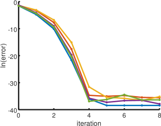
Figure 8. Logarithm of distance to $\mathbf{0}$ as a function of the iteration step for several runs of the algorithm for $A(x,y,z,u,v)$ given by equation (43). Several independent runs are plotted, each beginning at a random point in $[-0.2,0.2]^{5}$.

To demonstrate the performance of our method in locating a triple multiplicity, we consider the function

(43) $$A=\begin{pmatrix}1+v+w+x-3y-z&2x+y+2z&x+xz+y\\ 2x+y+2z&1+x+yz&2v-w+z\\ x+xz+y&2v-w+z&1+vw\end{pmatrix}$$

with triple eigenvalue at $(0,0,0,0,0)$. The results of several runs are shown in Figure 8; the convergence is clearly quadratic until the limit of numerical precision is reached in about 4 steps.

References

- [1] V. I. Arnold. Mathematical methods of classical mechanics. Springer-Verlag, New York, 1978. Translated from the Russian by K. Vogtmann and A. Weinstein, Graduate Texts in Mathematics, 60.
- [2] N. W. Ashcroft and N. D. Mermin. Solid State Physics. Holt, Rinehart and Winston, New York-London, 1976.
- [3] G. Berkolaiko. An elementary introduction to quantum graphs. In A. Girouard, D. Jakobson, M. Levitin, N. Nigam, I. Polterovich, and F. Rochon, editors, Geometric and Computational Spectral Theory, volume 700 of Contemporary Mathematics, pages 41–72. AMS, 2017. preprint arXiv:1603.07356.
- [4] M. V. Berry. Quantal phase factors accompanying adiabatic changes. Proc. Roy. Soc. London Ser. A, 392(1802):45–57, 1984.
- [5] M. Born and V. Fock. Beweis des adiabatensatzes. Zeitschrift fur Physik, 51(3-4):165–180, Mar 1928.
- [6] A. Castro Neto, F. Guinea, N. Peres, K. Novoselov, and A. Geim. The electronic properties of graphene. Rev. Mod. Phys., 81:109–162, 2009.
- [7] M. Dana and K. D. Ikramov. On the codimension of the variety of symmetric matrices with multiple eigenvalues. Zap. Nauchn. Sem. S.-Peterburg. Otdel. Mat. Inst. Steklov. (POMI), 323(Chisl. Metody i Vopr. Organ. Vychisl. 18):34–46, 224, 2005.
- [8] L. Dieci, A. Papini, and A. Pugliese. Approximating coalescing points for eigenvalues of Hermitian matrices of three parameters. SIAM J. Matrix Anal. Appl., 34(2):519–541, 2013.
- [9] L. Dieci and A. Pugliese. Singular values of two-parameter matrices: an algorithm to accurately find their intersections. Math. Comput. Simulation, 79(4):1255–1269, 2008.
- [10] L. Dieci and A. Pugliese. Two-parameter SVD: coalescing singular values and periodicity. SIAM J. Matrix Anal. Appl., 31(2):375–403, 2009.
- [11] L. Dieci and A. Pugliese. Hermitian matrices depending on three parameters: coalescing eigenvalues. Linear Algebra Appl., 436(11):4120–4142, 2012.
- [12] C. L. Fefferman and M. I. Weinstein. Wave packets in honeycomb structures and two-dimensional Dirac equations. Comm. Math. Phys., 326(1):251–286, 2014.
- [13] H. Gingold. A method of global blockdiagonalization for matrix-valued functions. SIAM J. Math. Anal., 9(6):1076–1082, 1978.
- [14] G. Herzberg and H. C. Longuet-Higgins. Intersection of potential energy surfaces in poluatomic molecules. Discuss. Faraday Soc., 35:77–82, 1963.
- [15] P. D. Hislop and I. M. Sigal. Introduction to spectral theory, volume 113 of Applied Mathematical Sciences. Springer-Verlag, New York, 1996. With applications to Schrödinger operators.
- [16] P.-f. Hsieh and Y. Sibuya. A global analysis of matrices of functions of several variables. J. Math. Anal. Appl., 14:332–340, 1966.
- [17] N. V. Ilyushechkin. The discriminant of the characteristic polynomial of a normal matrix. Mat. Zametki, 51(3):16–23, 143, 1992.
- [18] T. Kato. Perturbation theory for linear operators. Classics in Mathematics. Springer-Verlag, Berlin, 1995. Reprint of the 1980 edition.
- [19] P. Kuchment. Floquet theory for partial differential equations, volume 60 of Operator Theory: Advances and Applications. Birkhäuser Verlag, Basel, 1993.
- [20] P. Kuchment. An overview of periodic elliptic operators. Bull. Amer. Math. Soc. (N.S.), 53(3):343–414, 2016.
- [21] P. D. Lax. On the discriminant of real symmetric matrices. Comm. Pure Appl. Math., 51(11-12):1387–1396, 1998.
- [22] G. Montambaux, F. Piéchon, J.-N. Fuchs, and M. O. Goerbig. Merging of dirac points in a two-dimensional crystal. Phys. Rev. B, 80:153412, 2009.
- [23] K. Novoselov. Nobel lecture: Graphene: Materials in the flatland. Rev. Mod.Phys., 83:837–849, 2011.
- [24] K. A. O’Neil. Critical points of the singular value decomposition. SIAM J. Matrix Anal. Appl., 27(2):459–473, 2005.
- [25] B. N. Parlett. The (matrix) discriminant as a determinant. Linear Algebra Appl., 355:85–101, 2002.
- [26] A. Pugliese. Theoretical and numerical aspects of coalescing of eigenvalues and singular values of parameter dependent matrices. PhD thesis, Georgia Institute of Technology, 2008.
- [27] B. Simon. Holonomy, the quantum adiabatic theorem, and Berry’s phase. Phys. Rev. Lett., 51(24):2167–2170, 1983.
- [28] L. Tarruell, D. Greif, T. Uehlinger, G. Jotzu, and T. Esslinger. Creating, moving and merging Dirac points with a Fermi gas in a tunable honeycomb lattice. Nature, 483(7389):302–305, 2012.
- [29] J. von Neuman and E. Wigner. Uber merkwürdige diskrete Eigenwerte. Uber das Verhalten von Eigenwerten bei adiabatischen Prozessen. Physikalische Zeitschrift, 30:467–470, Jan 1929.