Effects of fluctuations on correlation functions in inhomogeneous mixtures

Abstract

Approximate expressions for correlation functions in binary inhomogeneous mixtures are derived in a framework of the mesoscopic theory [Ciach A., Mol. Phys., 2011, 109, 1101]. Fluctuation contribution is taken into account in a Brazovskii-type approximation. Explicit results are obtained for two model systems. In the two models, the diameters of the hard cores of particles are equal, and the interactions favour a periodic arrangement of alternating species A and B. However, the optimal distance between the species A and B is much different in the two models. Theoretical results for different temperature and volume fractions of the two components are compared with the results of Monte Carlo simulations, and the structure is illustrated by simulation snapshots. Despite different interaction potentials and different length scale of the local ordering, properties of the correlation functions in the two models are very similar.

Key words: correlation functions, inhomogeneous mixtures, mesoscopic theory

Abstract

 ðàìêàõ ìåçîñêîïiчíî¿ òåîði¿ [A. Ciach, Mol. Phys., 2011, 109, 1101] âèâåäåíî íàáëèæåíi âèðàçè äëÿ êîðåëÿöiéíèõ ôóíêöié â áiíàðíèõ íåîäíîðiäíèõ ñóìiøàõ. Ôëóêòóàöiéíèé âíåñîê âðàõîâóєòüñÿ â íàáëèæåííi Áðàçîâñüêîãî. Îòðèìàíî ÿâíi ðåçóëüòàòè äëÿ äâîõ ìîäåëüíèõ ñèñòåì.  îáîõ ìîäåëÿõ, äiàìåòðè òâåðäîãî êîðó чàñòèíîê є îäíàêîâèìè, à âçàєìîäi¿ ñïðèÿþòü ïåðiîäèчíîìó чåðãóâàííþ â ðîçòàøóâàííi ñîðòiâ A i B. Ïðîòå, îïòèìàëüíà âiäñòàíü ìiæ ñîðòàìè A i B ñóòòєâî ðiçíèòüñÿ â äâîõ ìîäåëÿõ. Òåîðåòèчíi ðåçóëüòàòè äëÿ ðiçíèõ çíàчåíü òåìïåðàòóðè i îá’єìíèõ ôðàêöié äâîõ êîìïîíåíò ïîðiâíþþòüñÿ ç ðåçóëüòàòàìè ìîäåëþâàííÿ ìåòîäîì Ìîíòå Êàðëî, à ñòðóêòóðè ïðîiëþñòðîâàíi ìèòòєâèìè çíèìêàìè ñèñòåìè. Íåçâàæàþчè íà òå, ùî ïîòåíöiàëè âçàєìîäi¿ i ìàñøòàáè ëîêàëüíîãî âïîðÿäêóâàííÿ â äâîõ ìîäåëÿõ є ðiçíèìè, âëàñòèâîñòi êîðåëÿöiéíèõ ôóíêöié öèõ ìîäåëåé є äóæå ïîäiáíèìè.

Ключовi слова: êîðåëÿöiéíi ôóíêöi¿, íåîäíîðiäíi ñóìiøi, ìåçîñêîïiчíà òåîðiÿ

1 Introduction

Biological and soft-matter systems are typically multicomponent and inhomogeneous. For different systems, the inhomogeneities in density or concentration may appear on different length scales, ranging from the scale set by the size of molecules through a few- to a few tens or even hundreds of molecular diameters. For example, in ionic systems or in two-component mixtures of highly charged colloid particles, the concentration difference between the positively and negatively charged ions or particles oscillates in space in the crystalline phases on the length scale set by the size of the ions or particles [1, 2]. In ionic liquids (IL) or molten colloidal crystals, the inhomogeneities remain present, and are reflected in the oscillatory decay of the correlation function for the concentration difference (or charge density) on the same length scale  [3, 4, 5, 6]. In this case, the inhomogeneity or local order actually means that the distribution of the components in the majority of microscopic states in the disordered phase differs significantly from the random distribution.

In the case of weakly charged colloid particles with solvent-induced effective short-range attraction, clusters of particles of various sizes and shapes or other assemblies are formed, which leads to inhomogeneities on a mesoscopic length scale [7, 8, 9, 10, 11, 12]. Similar inhomogeneities or self-assembly into different aggregates can occur in other systems with interactions between the particles of the form of the so-called ‘mermaid’ or SALR potential [13], for example in globular proteins in water [7, 14, 15]. In the SALR class of potentials, the interactions consist of short range attraction (SA) and long-range repulsion (LR). At low temperature, a universal sequence of the ordered phases (lyotropic liquid crystals) was predicted  [16, 17, 18, 19] and was found in simulations [20] for increasing the volume fraction of the particles. When the density increases, there is observed the formation of a cluster crystal of cubic symmetry, hexagonal arrangement of cylindrical clusters, gyroid network of particles, lamellas, gyroid network of voids, cylindrical voids and spherical voids. When the ordered phases melt, the aggregates start to move freely leading to position-independent density. The local order is reflected in the oscillatory decay of correlations on the length scale set by the size of the aggregates. Importantly, even though the average density is position independent, almost all simulation snapshots show the formation of aggregates [9, 12, 11]. The random distribution of particles is not observed in practice. Only at high temperature, the aggregates become disintegrated, and the random structure domintes in the microscopic states of the disordered phase. In a fixed mesoscopic window of the macroscopic volume, the density is either much larger or much smaller than the average density, when an aggregate either enters or leaves the window. This means that very large fluctuations of the local density take place. As a result, the internal energy obtained by a proper averaging of the energy of the microscopic states differs significantly from the energy calculated in the mean-field (MF) approximation, i.e., for the average density. This is because when the aggregates of a size determined by the range of attraction are separated by distances larger than the range of repulsion, there are much more pairs of attracting particles and much less pairs of particles that repel each other than in the state with a position-independent density (homogeneously distributed particles). That is why the energy of the majority of states in the inhomogeneous disordered phase is much lower than the energy calculated for the disordered phase in MF. The latter is the same for homogeneous and inhomogeneous systems. The much overestimated internal energy leads to instability of the disordered phase with respect to density modulations, and to a continuous phase transition in MF that in reality is absent. The spurious instability of the disordered inhomogeneous phase in MF leads to divergent correlation functions that in reality do not diverge. Mesoscopic fluctuations of the local density, representing a different density inside the clusters and between them, i.e., the variance of the local density or concentration, should be taken into account to restore the stability of the disordered inhomogeneous phase and to lead correct correlation functions and the first-order phase transition to the ordered phases at lower temperature.

The effects of mesoscopic fluctuations can be taken into account within the field-theory developed by Brazovskii [21]. This theory was adapted to amphiphilic systems in [22, 23]. A mesoscopic density-functional theory with the variance of the local density taken into account in the approach based on the Brazovskii theory was developed in [16, 17, 24] for one-component systems, and in [25] for mixtures. A similar approach was used for the study of ionic systems in  [5, 6, 26].

At the formal level, the variance of the local density can be obtained by solving the self-consistent equation for the inverse correlation function in the one-loop Hartree approximation [16, 27, 24]. The contribution to the grand potential associated with the presence of inhomogeneities is calculated at the same level of approximation. From the physical point of view, the variance of the local volume fraction describes the average deviation of the volume fraction inside the clusters or between them from the volume fraction averaged over the whole volume. This average inhomogeneity leads to a negative contribution to the internal energy, and to stabilization of the disordered phase for a much larger part of the phase diagram than in MF. In a one-component system, this theory leads to a correct high-$T$ part of the phase diagram at a semi-quantitative level [24]. The mathematical form of the correlation function for the volume fraction in this theory is the same as in MF, namely

$$G(r)=A\mathrm{e}^{-\alpha_{0}r}\sin(\alpha_{1}r+\theta)/r,$$ (1.1)

but the dependence of the parameters on thermodynamic state is much different: there is no spurious divergence of $A$ or $1/\alpha_{0}$. Equation (1.1) should describe the asymptotic decay of correlations when the correlation function in Fourier representation, $\tilde{G}(k)$, takes a maximum for $k=k_{0}>0$ even in the exact theory. It can be obtained from the pole analysis of $\tilde{G}(k)$, by taking into account the pair of poles $\mathrm{i}\alpha_{0}\pm\alpha_{1}$ with the smallest imaginary part. However, simulations show that equation (1.1) very well describes the correlation function for the volume fraction or for the charge density in the SALR or IL systems already for $r$ larger than one period of the damped oscillations [12, 28].

Much less attention was paid to inhomogeneous mixtures. In [25], only the general formalism has been developed, and a few examples were considered only in MF. In this article we focus on the structure of the disordered inhomogeneous phase described by correlation functions for different components. In section 2, we briefly summarize the Brazovskii-type formalism generalized to mixtures in [25]. Next, we restrict ourselves to binary mixtures and derive approximate equations for the correlation functions in Fourier representation, $\tilde{G}_{\alpha\beta}(k)$. We restrict ourselves to equal sizes of the hard cores of the particles, and consider two particular examples of a binary mixture. In the first example, section 3, we assume interactions leading to inhomogeneities on a length scale of $\sim 10\sigma$, where $\sigma$ is a molecular size. We choose the ‘mermaid’ potential between the like particles, but a pair of different particles interact with a ‘peacock’ potential having an attractive tail and a repulsive head. The tails of the interactions correspond to screened electrostatic potentials (repulsion between the like-particles, and attraction between the opposite charges) and the short-range part of the interactions favours a phase separation of the two species. ‘Two mermaids and a peacock’ effective interactions can occur between oppositely charged hydrophilic and hydrophobic colloid particles suspended in a near-critical mixture with ions [29].

In section 4, we assume that short-range interactions of the square-well are formed only between different species. This potential can lead to a gas-liquid phase transition, as well as to the ordered phase resembling an ionic crystal, with the structure on the length scale of $\sigma$ [25]. We calculate three correlation functions in the disordered phase for several state points for two models both above and below the MF instability. In order to verify the theoretical predictions and to visualize the structure for different state points, we have performed MC simulations for the models considered. We conclude in section 5.

2 Formalism

The theory is based on the mesoscopic formalism developed for inhomogeneous mixtures with $n$ components in [25]. Instead of the number density $\rho_{\alpha}$ of the $\alpha$-component, we consider the volume fraction in the mesoscopic region around ${\bf r}$, $\zeta_{\alpha}({\bf r})$, and deviations $\Delta\zeta_{\alpha}({\bf r})$ from the average value, $\bar{\zeta}_{\alpha}({\bf r})$. The volume fraction is more suitable in the mesoscopic theory, particularly for unequal sizes of the particles. When the ordering occurs on the length scale much larger than the size of the particles, then the volume fraction and the number density of the particles with the volume $v_{\alpha}$ are related by $\zeta_{\alpha}\approx\rho_{\alpha}v_{\alpha}$.

Fixed forms of the local volume fractions of all the components, $\{\zeta\}=(\zeta_{1},\ldots,\zeta_{n})$, can be considered as a constraint imposed on the microscopic states. Grand potential in the presence of the above mesoscopic constraint can be written in the form $\Omega_{\text{co}}=U-TS-\mu_{\alpha}N_{\alpha}$, where $U,S,N_{\alpha}$ and $\mu_{\alpha}$ are the internal energy, entropy, the number of molecules and the chemical potential of the species $\alpha$ respectively in the system with the constraint of fixed $\{\zeta\}$ imposed on the microscopic densities. $U$ is given by the expression

$$U[\{\zeta\}]=\frac{1}{2}\int_{\bf r_{1}}\int_{\bf r_{2}}\bar{V}_{\alpha\beta}(|{\bf r}_{1}-{\bf r}_{2}|)\zeta_{\alpha}({\bf r}_{1})\zeta_{\beta}({\bf r}_{2}),$$

where the element $\bar{V}_{\alpha\beta}(r)$ of the matrix $\bar{\bf V}(r)$ is the interaction potential between the species $\alpha,\beta$, properly rescaled when the volume fraction instead of the number density is considered. In addition, the interaction potentials are multiplied by the function that vanishes for $r=|{\bf r}_{1}-{\bf r}_{2}|$ smaller than the sum of the hard-cores radii, and is equal to 1 otherwise. This way we avoid contributions to the internal energy from the states with overlapping cores of the particles. We further assume that the entropy $S$ satisfies the relation $-TS=F_{\text{h}}$, where $F_{\text{h}}$ is the free-energy of the hard-core reference system. We assume here a local-density approximation.

In this work we study the effects of fluctuations on the correlation functions ${\bf G}$, with the matrix elements $G_{\alpha\beta}({\bf r}_{\alpha},{\bf r}_{\beta})=\langle\Delta\zeta_{\alpha}({\bf r}_{\alpha})\Delta\zeta_{\beta}({\bf r}_{\beta})\rangle$ representing the correlations between the volume fractions of the species $\alpha$ and $\beta$ at the positions ${\bf r}_{\alpha}$ and ${\bf r}_{\beta}$, respectively. In order to include fluctuations, we introduce the functional $\beta F[\{\zeta\}]$ of the form

$$\beta F[\{\zeta\}]=\beta\Omega_{\text{co}}[\{\zeta\}]-\log\left[\int\text{D}\phi_{1}\ldots\int\text{D}\phi_{n}\mathrm{e}^{-\beta H_{\text{fluc}}}\right],$$ (2.1)

where $\phi_{\alpha}({\bf r})$ is the local fluctuation of the volume fraction of the component $\alpha$, and

$$H_{\text{fluc}}[\{\zeta\},\{\phi\}]=\Omega_{\text{co}}[\{\zeta\}+\{\phi\}]-\Omega_{\text{co}}[\{\zeta\}].$$

The functional (2.1) becomes equal to the grand potential, when $\{\zeta\}=\{\bar{\zeta}\}$, with $\{\bar{\zeta}\}=[\bar{\zeta}_{\alpha_{1}}({\bf r}),\ldots,\bar{\zeta}_{\alpha_{n}}({\bf r})]$ that satisfy the minimum condition for (2.1). By definition, $\langle\phi_{\alpha}\rangle=0$ when $\{\zeta\}=\{\bar{\zeta}\}$.

Note that from (2.1) it follows that the vertex functions (related to the direct correlation functions) defined by

$${\cal C}_{\alpha_{1},\ldots,\alpha_{j}}({\bf r}_{1},\ldots,{\bf r}_{j})=\frac{\delta^{j}\beta F[\{\bar{\zeta}\}]}{\delta\bar{\zeta}_{\alpha_{1}}({\bf r}_{1})\ldots\delta\bar{\zeta}_{\alpha_{j}}({\bf r}_{j})}$$

consist of two terms: the first one is the contribution from the fluctuations on the microscopic length scale with frozen fluctuations on the mesoscopic length scale. This term is

$${\cal C}^{\text{co}}_{\alpha_{1},\ldots,\alpha_{j}}({\bf r}_{1},\ldots,{\bf r}_{j})=\frac{\delta^{j}\beta\Omega_{\text{co}}[\{\bar{\zeta}\}]}{\delta\bar{\zeta}_{\alpha_{1}}({\bf r}_{1})\ldots\delta\bar{\zeta}_{\alpha_{j}}({\bf r}_{j})}.$$ (2.2)

The second term is the contribution from the fluctuations on the mesoscopic length scale.

We focus on the two-point inverse correlation function that satisfies the analog to the Ornstein-Zernicke equation,

$${\bf C}={\bf G}^{-1}.$$ (2.3)

In the lowest-order nontrivial approximation, the matrix elements of the inverse correlation function in Fourier representation are given by [25],

$$\tilde{C}_{\alpha\beta}(k)=\tilde{C}^{\text{co}}_{\alpha\beta}(k)+\frac{A_{\alpha\beta\gamma\delta}}{2}{\cal G}_{\gamma\delta}\,,$$ (2.4)

where the first term is the function defined in (2.2) with $j=2$ in Fourier representation, summation convention is used in the whole article, and

$${\cal G}_{\gamma\delta}=\int\frac{\mathrm{d}{\bf k}}{(2\piup)^{3}}\tilde{G}_{\gamma\delta}(k).$$ (2.5)

In the case of the disordered phase, $\tilde{C}^{\text{co}}_{\alpha\beta}(k)=\beta\tilde{V}_{\alpha\beta}(k)+A_{\alpha\beta}$. The matrix $\tilde{\bf V}(k)$ with the elements $\tilde{V}_{\alpha\beta}(k)$ is the interaction potential between the species $\alpha,\beta$ in Fourier representation, and $A_{\alpha_{1}\ldots\alpha_{j}}$ is given by

$$A_{\alpha_{1}\ldots\alpha_{j}}=\frac{\partial^{j}\beta f_{\text{h}}(\{\zeta({\bf r})\})}{\partial\zeta_{\alpha_{1}}({\bf r})\ldots\partial\zeta_{\alpha_{j}}({\bf r})}.$$

Equations (2.3)–(2.5) should be solved self-consistently, which is not an easy task, especially for periodic structures in multicomponent mixtures.

In this work we focus on a disordered inhomogeneous phase in a binary mixture, with $\alpha,\beta=1,2$. Inhomogeneities at the mesoscopic length scale indicate that the correlation functions in Fourier representation take a maximum for $0<k<2\piup$. We assume that the inhomogeneities occur on a well-defined length scale, and the peak of $\tilde{G}_{\gamma\delta}(k)$ is high and narrow.

Let us consider

$${\cal G}_{\alpha\beta}=\int\frac{\mathrm{d}{\bf k}}{(2\piup)^{3}}\frac{[\tilde{C}_{\alpha\beta}(k)]}{\det\tilde{\bf C}(k)}\,,$$ (2.6)

where $[\tilde{C}_{\alpha\alpha}(k)]=\tilde{C}_{\beta\beta}(k)$ and $[\tilde{C}_{\alpha\beta}(k)]=-\tilde{C}_{\alpha\beta}(k)$ for $\alpha\neq\beta$. By symmetry, $\tilde{C}_{12}=\tilde{C}_{21}$. For the considered functions with a high, narrow peak, the main contribution to the integral comes from the vicinity of the maximum. In general, $\tilde{C}_{\alpha\beta}(k)/\det\tilde{\bf C}(k)$ can take the maximum for different values of $k$ for different pairs of $\alpha,\beta$. Here, we focus on the case where the maximum of all the integrands in (2.6) is very close to the minimum at $k=k_{0}$ of $\det\tilde{\bf C}(k)$, and we can make the approximation

$${\cal G}_{\alpha\beta}=[\tilde{C}_{\alpha\beta}(k_{0})]{\cal G},$$

where

$${\cal G}=\int\frac{\mathrm{d}{\bf k}}{(2\piup)^{3}}\frac{1}{\det\tilde{\bf C}(k)}.$$ (2.7)

In the Brazovskii-type theory considered here, the $k$ dependence of $\tilde{C}_{\alpha\beta}$ comes only from $\tilde{V}_{\alpha\beta}(k)$, and we can write (2.4) in the form

$$\tilde{\bf C}(k)=\beta\tilde{\bf V}(k)+{\bf c}\,,$$ (2.8)

where the elements $c_{\alpha\beta}$ of ${\bf c}$ are

$$c_{\alpha\beta}=A_{\alpha\beta}+\frac{A_{\alpha\beta\gamma\delta}}{2}{\cal G}_{\gamma\delta}.$$

We introduce the notation

$$\det\tilde{\bf C}(k)=\det{\bf c}+\beta\tilde{W}(k),$$ (2.9)

with

$$\beta\tilde{W}(k)=\beta\Big{[}\beta\det\tilde{\bf V}(k)+\tilde{V}_{11}(k)c_{22}+\tilde{V}_{22}(k)c_{11}-2\tilde{V}_{12}(k)c_{12}\Big{]}.$$ (2.10)

Close to a deep minimum, we can make the expansion

$$\det\tilde{\bf C}(k)=D_{0}+\frac{\beta\tilde{W}^{\prime\prime}(k_{0})}{2}(k-k_{0})^{2}+\ldots\,,$$ (2.11)

where $k_{0}$ is determined by the equation

$$\beta\tilde{W}^{\prime}(k_{0})=0$$ (2.12)

and

$$D_{0}=\det\tilde{\bf C}(k_{0}).$$ (2.13)

From the approximation (2.11) and (2.7), we obtain [25, 27]

$${\cal G}\approx\frac{k_{0}^{2}}{\piup\sqrt{2\beta\tilde{W}^{\prime\prime}(k_{0})D_{0}}}.$$ (2.14)

In order to obtain an explicit equation for $k_{0}$, we take into account that from (2.8) it follows that ${\bf c}=\tilde{\bf C}(k_{0})-\beta\tilde{\bf V}(k_{0})$. From the above and (2.12), (2.10) we obtain the equation

$$\tilde{V}_{11}^{\prime}(k_{0})\tilde{C}_{22}(k_{0})+\tilde{V}_{22}^{\prime}(k_{0})\tilde{C}_{11}(k_{0})-2\tilde{V}_{12}^{\prime}(k_{0})\tilde{C}_{12}(k_{0})=0$$ (2.15)

that contains the 3 unknowns $\tilde{C}_{\alpha\beta}(k_{0})$. $D_{0}$ is expressed in terms of the above unknowns [see (2.13)], and finally

$$\tilde{W}^{\prime\prime}(k_{0})=2\beta\det\tilde{\bf V}^{\prime}(k_{0})+\tilde{V}_{11}^{\prime\prime}(k_{0})\tilde{C}_{22}(k_{0})+\tilde{V}_{22}^{\prime\prime}(k_{0})\tilde{C}_{11}(k_{0})-2\tilde{V}_{12}^{\prime\prime}(k_{0})\tilde{C}_{12}(k_{0}).$$ (2.16)

In order to determine ${\bf C}$ in this approximation from (2.8), we need 3 equations in addition to equation (2.15), because we have 4 unknowns, $k_{0}$ and $\tilde{C}_{\alpha\beta}(k_{0})$. Using (2.4), (2.14), (2.13) and (2.16) we obtain 3 equations with the unknowns $k_{0}$ and $\tilde{C}_{\alpha\beta}(k_{0})$,

$$\tilde{C}_{\alpha\beta}(k_{0})=\beta\tilde{V}_{\alpha\beta}(k_{0})+A_{\alpha\beta}+\frac{k_{0}^{2}A_{\alpha\beta\gamma\delta}[\tilde{C}_{\gamma\delta}(k_{0})]}{2\piup\sqrt{2\beta\tilde{W}^{\prime\prime}(k_{0})D_{0}}}.$$ (2.17)

Equations (2.15) and (2.17) form a closed set of 4 equations for 4 unknowns, when the expressions (2.13) and (2.16) for $D_{0}$ and $\tilde{W}^{\prime\prime}$ are used, and $[\tilde{C}_{\gamma\delta}(k_{0})]$ are defined below (2.6).

Once $\tilde{C}_{\alpha\beta}(k_{0})$ are determined, the correlation functions can be obtained from the equation

$$\tilde{C}_{\alpha\beta}(k)=\tilde{C}_{\alpha\beta}(k_{0})+\beta[\tilde{V}_{\alpha\beta}(k)-\tilde{V}_{\alpha\beta}(k_{0})].$$ (2.18)

The approximate expression (2.14) is valid only when the correlation functions in Fourier representation have a pronounced maximum at $k=k_{0}$. In such a case, $\tilde{V}_{\alpha\beta}(k)-\tilde{V}_{\alpha\beta}(k_{0})$ in (2.18) can be expanded about $k_{0}$, and the expansion can be truncated. We should stress that the theory is not valid at high temperature, where no inhomogeneities at a well defined length scale are present.

In the next two sections we consider a binary mixture and assume the same size of the spherical hard cores of the particles of the two kinds. For the free energy of the hard-sphere reference system we assume $F_{\text{h}}=\int\mathrm{d}{\bf r}f_{\text{h}}[\zeta_{1}({\bf r}),\zeta_{2}({\bf r})]$ with the Carnahan-Starling approximation for the free energy density $f_{\text{h}}(\zeta_{1},\zeta_{2})=\zeta_{1}\ln\zeta_{1}+\zeta_{2}\ln\zeta_{2}+f_{\text{ex}}(\zeta)$, where $\zeta=\zeta_{1}+\zeta_{2}$ and

$$f_{\text{ex}}(\zeta)=\frac{6\zeta}{\piup}\left[\frac{4\zeta-3\zeta^{2}}{(1-\zeta)^{2}}-1\right].$$

For equal sizes, we have $A_{12}=A_{2}(\zeta)$, $A_{1112}=A_{1122}=A_{1222}=A_{4}(\zeta)$, and $A_{\alpha\alpha}=A_{2}(\zeta)+1/\zeta_{\alpha}$, $A_{\alpha\alpha\alpha\alpha}=A_{4}(\zeta)+2/\zeta_{\alpha}^{3}$, where $A_{n}(\zeta)=\mathrm{d}^{n}f_{\text{ex}}(\zeta)/\mathrm{d}^{n}\zeta$. We use the diameter of the particles as the length unit.

We assume different interaction potentials that can lead to different inhomogeneities on different length scales.

3 The case of interaction potentials $V_{11}=V_{22}=-V_{12}=V$

In this section we assume interaction potentials that are a simplified version of the interactions between charged colloid particles of equal sizes but of different sign of the charge, and different chemistry of the two species. For example, the species 1 can be ‘hydrophilic’, while the species 2 ‘hydrophobic’. The like-particles attract each other at short distances due to a similar chemistry, but at large distances they repel each other because of the screened electrostatic repulsion between like charges. Particles of a different kind attract each other at large distances due to the screened electrostatic potential between opposite charges. We assume the short-range repulsion to enhance the tendency for demixing of uncharged particles. This kind of interactions between the like-particles is known as a ‘mermaid’ or SALR potential. Note that $V_{12}$ is repulsive at short distances and attractive at large distances, i.e., it has a repulsive head and a attractive tail (like a peacock). In experiment, the ‘two mermaids and a peacock’ effective interactions can be obtained when the oppositely charged hydrophilic and hydrophobic colloid particles are immersed in a near-critical mixture of water and oil, for example lutidine. Critical concentration fluctuations lead to the Casimir potential between confining surfaces [29]. This potential is attractive for the like-surfaces, and repulsive between the hydrophilic and the hydrophobic surface. The range of the Casimir potential, equal to the bulk correlation length, $\xi_{\text{b}}$, can be tuned by temperature. When $\xi_{\text{b}}$ is smaller than the Debye length of the screened electrostatic potential, and the charge of the particles is properly chosen, the ‘two mermaid and a peacock’ potential can be created.

3.1 Theory

To simplify the calculations, we assume that the interactions between the like-particles are the same in this model, $V_{11}=V_{22}=V$, and for a different kind of particles we assume $V_{12}=V_{21}=-V$. In our mesoscopic theory $V(r)=0$ for $r<1$, and for $r>1$ we assume the double-Yukava potential with short-range attraction and long-range repulsion,

$$V(r)=-\frac{K_{1}}{r}\mathrm{e}^{-\kappa_{1}r}+\frac{K_{2}}{r}\mathrm{e}^{-\kappa_{2}r}.$$ (3.1)

Here, we do not try to model any particular system. Our aim is to verify the predictions of the mesoscopic theory for the case of inhomogeneities present at the length scale larger than the size of the particles. We choose $K_{1}=1,K_{2}=0.2,\kappa_{1}=1,\kappa_{2}=0.5$ that leads to relatively large clusters, with diameter $\sim 5\sigma$. The amplitude of the attractive part of $V$ sets the energy unit, and we use the dimensionless temperature $T^{*}=k_{\text{B}}T/K_{1}$. The high symmetry of the interaction potentials greately simplifies the calculations.

In MF, after some algebra we obtain the following expressions for the correlation functions in Fourier representation (proportional to structure factors)

$$\tilde{G}_{11}^{\text{co}} =G_{0}+\frac{(\zeta+c)^{2}[1+2A_{2}(\zeta-c)]^{2}}{D^{\text{co}}(k)}\,,$$

$$\tilde{G}_{22}^{\text{co}} =G_{0}+\frac{(\zeta-c)^{2}[1+2A_{2}(\zeta+c)]^{2}}{D^{\text{co}}(k)}\,,$$

$$\tilde{G}_{12}^{\text{co}} =G_{0}-\frac{(\zeta^{2}-c^{2})\left[(1+A_{2}\zeta)^{2}-A_{2}^{2}c^{2}\right]}{D^{\text{co}}(k)}\,,$$

where the constant term leading to the Dirac delta function in real space is

$$G_{0}=\frac{\zeta(1-c^{2}/\zeta^{2})}{4[1+A_{2}\zeta(1-c^{2}/\zeta^{2})]}\,,$$

$$D^{\text{co}}(k)=4(1+A_{2}\zeta)^{2}\zeta\left[1-\frac{A_{2}c^{2}}{\zeta(1+A_{2}\zeta)}\right]\left\{1+\zeta\left[1-\frac{A_{2}c^{2}}{\zeta(1+A_{2}\zeta)}\right]\right\},$$ (3.2)

$\tilde{V}(k)$ is the interaction potential (3.1) in Fourier representation with the explicit expression given for example in [30], and we have introduced $c=\zeta_{1}-\zeta_{2}$.

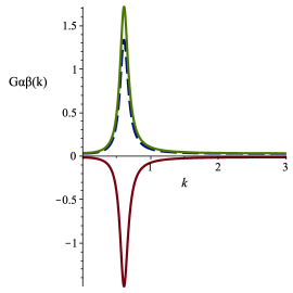
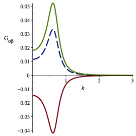
Figure 1: (Colour online) Correlation functions in Fourier representation for $T^{*}=0.28$, $\zeta=0.1$ and $c=0.02$ in MF (left-hand panel) and with the effect of fluctuations taken into account (right-hand panel). Upper solid lines: $\tilde{G}_{11}(k)$, dashed lines: $\tilde{G}_{22}(k)$, and lower solid lines: $\tilde{G}_{12}(k)$.

In MF, the disordered phase becomes unstable with respect to oscillatory modulations of the volume fractions at the $\lambda$-surface given by

$$T^{*}(\zeta,c)=-\tilde{V}(k_{0})\zeta\left\{1-\frac{A_{2}(\zeta)c^{2}}{\zeta[1+A_{2}(\zeta)\zeta]}\right\},$$

therefore, we restrict ourselves to $T^{*}$ above the $\lambda$-surface, i.e., to the stability region of the disordered phase. Because of the symmetry of interactions, we assume that the majority component is the species 1, and consider only $c>0$. The correlation functions, $\tilde{G}_{\alpha\beta}^{\text{co}}(k)$, are shown in figure 1 for $T^{*}=0.28$, total volume fraction of the particles $\zeta=\zeta_{1}+\zeta_{2}=0.1$, and the difference in the volume fractions of the two species $c=\zeta_{1}-\zeta_{2}=0.02$. The maximum of $\tilde{G}_{\alpha\alpha}(k)$ or a minimum of $\tilde{G}_{12}(k)$ is assumed for $k=k_{0}\approx 0.609$ which corresponds to the minimum of $\tilde{V}(k)$. The period of damped oscillations in real space is $\sim 2\piup/k_{0}\approx 10.3$. In figure 2 we show $\tilde{G}_{\alpha\beta}^{\text{co}}(k_{0})$. Due to the symmetry, $\tilde{G}_{11}^{\text{co}}=\tilde{G}_{22}^{\text{co}}$ for $c=0$. When $c\neq 0$, the structure factor of the majority component is larger than the structure factor of the minority component, and the difference increases with an increasing asymmetry (see figure 2). Somewhat surprisingly, the maximum of $\tilde{G}_{11}^{\text{co}}(k_{0})$ as a function of $c$ is assumed for slightly different volume fractions of the two components, i.e., for $c=0.01$ which corresponds to $\zeta_{1}=0.055$ and $\zeta_{2}=0.045$. For larger asymmetries, all the correlations decrease with an increasing $c$.

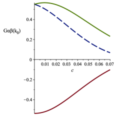
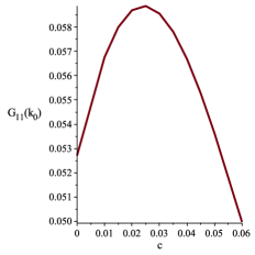
Figure 2: (Colour online) Left-hand panel: $\tilde{G}_{11}(k_{0})$ (upper solid line), $\tilde{G}_{22}(k_{0})$ (dashed line) and $\tilde{G}_{12}(k_{0})$ (lower solid line) in MF. Right-hand panel: $\tilde{G}_{11}(k_{0})$ with the effect of fluctuations taken into account. $\tilde{G}_{22}(k_{0})$ and $\tilde{G}_{12}(k_{0})$ are monotonous functions of $c$. $T^{*}=0.28$, $\zeta=0.1$ and $c$ is the difference in the volume fraction of the species 1 and 2.

Let us focus on the effects of fluctuations. Because of the assumed symmetry of interactions, we have $\det\tilde{\bf V}(k)=0$, and from equations (2.9)–(2.12) we can see that the minimum of $\det\tilde{\bf C}(k)$ is taken for the same value of $k$ as the minimum of $\tilde{V}(k)$. Thus, $k_{0}$ is not shifted in this model in the presence of fluctuations. Moreover, equation (2.16) simplifies to $W^{\prime\prime}(k_{0})=\tilde{V}^{\prime\prime}(k_{0})P$, where

$$P=\tilde{C}_{11}(k_{0})+\tilde{C}_{22}(k_{0})+2\tilde{C}_{12}(k_{0}).$$ (3.3)

The correlation functions in the presence of fluctuations in the Brazovskii-type approximation after some algebra take the forms

$$\tilde{G}_{11} =P^{-1}+\frac{[\tilde{C}_{22}(k_{0})+\tilde{C}_{12}(k_{0})]^{2}}{D(k)}\,,\quad\tilde{G}_{22}=P^{-1}+\frac{[\tilde{C}_{11}(k_{0})+\tilde{C}_{12}(k_{0})]^{2}}{D(k)}\,,$$ (3.4)

$$\tilde{G}_{12} =P^{-1}-\frac{\tilde{C}_{11}(k_{0})\tilde{C}_{22}(k_{0})+\tilde{C}_{12}(k_{0})[\tilde{C}_{11}(k_{0})+\tilde{C}_{22}(k_{0})+\tilde{C}_{12}(k_{0})]}{D(k)}\,,$$ (3.5)

where $D(k)=P\{P[\beta\tilde{V}(k)-\beta\tilde{V}(k_{0})]+D_{0}\}$ with $D_{0}$ defined in (2.13). In order to calculate the correlation functions, we numerically solved the set of equations (2.17) for $\tilde{C}_{11}(k_{0})$, $\tilde{C}_{22}(k_{0})$, and $\tilde{C}_{12}(k_{0})$.

The correlation functions in this approximation, equations (3.4)–(3.5), are compared with the MF result in figure 1 for $T^{*}=0.28$, $\zeta=0.1$, and $c=0.02$. As expected, fluctuations lead to a much smaller amplitude and range of the correlation functions, especially near the $\lambda$-surface, where $\tilde{C}_{\alpha\beta}^{\text{co}}(k_{0})$ diverge in MF. This is manifested by a smaller value and a larger width of the peak of $\tilde{C}_{\alpha\beta}(k)$ compared to the MF result. The property that the correlations between particles of the majority component are stronger is still present. In figure 2 we show $\tilde{G}_{11}(k_{0})$ for $T^{*}=0.28$, $\zeta=0.1$ and for a range of $c$, with the fluctuation contribution included. The nonmonotonous dependence on $c$ is enhanced in the presence of fluctuations, and the maximum occurs for $c=0.02$. The magnitude of the other correlation functions decreases monotonously with an increasing $c$.

The peak of the correlation functions becomes higher and narrower for an increasing density and/or a decreasing temperature, signaling correlations stronger and of larger range. The effect of temperature can be seen by comparing figure 1 for $T^{*}=0.28$ with figure 3 for $T^{*}=0.12$, both for $\zeta=0.1$. In figure 3, the correlation functions are shown for $c=0.02$ and $c=0.06$. We can see a strong effect of the difference in concentrations of the species $1$ and $2$ on the correlation functions. All correlations decrease, but especially the minority component becomes much less correlated when its volume fraction decreases.

It is also interesting to consider the correlation function for the total volume fraction, $G({\bf r}_{1}-{\bf r}_{2})=\langle\Delta\zeta({\bf r}_{1})\Delta\zeta({\bf r}_{2})\rangle$. Equations (3.4)–(3.5) give

$$\tilde{G}(k)=4P^{-1}+\frac{\left[\tilde{C}_{22}(k_{0})-\tilde{C}_{11}(k_{0})\right]^{2}}{D(k)}.$$

This equation and figure 3 show that the correlations for the total volume fraction increase with an increasing asymmetry which in this case is induced by increasing $c$. In the fully symmetrical case, $\tilde{G}(k)$ vanishes in this theory.

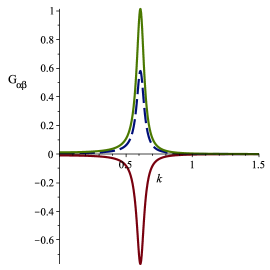
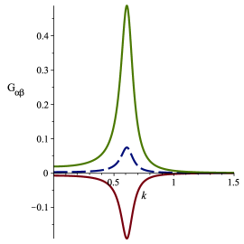
Figure 3: (Colour online) Correlation functions in Fourier representation for $T^{*}=0.12$ and $\zeta=0.1$ with the effect of fluctuations taken into account. Upper solid lines: $\tilde{G}_{11}(k)$, dashed lines: $\tilde{G}_{22}(k)$ and lower solid lines: $\tilde{G}_{12}(k)$. Left-hand panel: $c=0.02$. Right-hand panel: $c=0.06$.

If the assumptions leading to the fluctuation contribution obtained in the Brazovskii-type approximation are valid, we can make the approximation

$$\tilde{V}(k)-\tilde{V}(k_{0})\approx\frac{V^{\prime\prime}(k_{0})}{8k_{0}^{2}}(k^{2}-k_{0}^{2})^{2}\,,$$ (3.6)

where we took into account that $\tilde{G}_{\alpha\beta}(k)$ should be even functions of $k$. In this approximation, the correlation functions in real-space representation can be calculated analytically by inverse Fourier transforming equations (3.4)–(3.5). The results have the form (1.1) with $\theta=0$, and the inverse lengths $\alpha_{0},\alpha_{1}$ are given by

$$2\alpha_{0}^{2}=\left\{8k_{0}^{2}\left[\frac{k_{0}^{2}}{8}+\frac{T^{*}D_{0}}{P\tilde{V}^{\prime\prime}(k_{0})}\right]\right\}^{1/2}-k_{0}^{2}\,,\qquad 2\alpha_{1}^{2}=\left\{8k_{0}^{2}\left[\frac{k_{0}^{2}}{8}+\frac{T^{*}D_{0}}{P\tilde{V}^{\prime\prime}(k_{0})}\right]\right\}^{1/2}+k_{0}^{2}\,,$$

where $P$ and $D_{0}$ are defined in (3.3) and (2.13), respectively. In figure 4 we show the correlation functions in real space for $T^{*}=0.12$, $\zeta=0.1$ and $c=0.02$. The negative extremum of $\tilde{C}_{12}(k)$ at $k=k_{0}$ leads to the opposite signs of $C_{12}(r)$ and $C_{\alpha\alpha}(r)$ for the same value of $r$. This means that the regions enriched in one component are depleted in the other component.

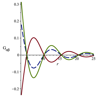
Figure 4: (Colour online) Correlation functions in real space for $T^{*}=0.12$, $\zeta=0.1$ and $c=0.02$ with the effect of fluctuations taken into account. $G_{11}(r)$ (green upper solid line on the left), $G_{22}(r)$ (dashed line) and $G_{12}(r)$ (red lower solid line on the left).

3.2 Simulations

A binary mixture of particles interacting with the SALR potential (3.1) with $K_{1}=1,K_{2}=0.2,\kappa_{1}=~{}1,\newline \kappa_{2}=0.5$ was simulated by applying a Monte Carlo technique in the $NVT$ ensemble. The particles had the same diameter ($\sigma_{1}=\sigma_{2}=\sigma=1.0$), and were placed in a cubic box of edge length $50\sigma$, with periodic boundary conditions applied to the system in the three directions. Cut-off radius was $15\sigma$. Each system had run $10^{6}$ Monte Carlo steps for equilibration and $10^{5}$ for production.

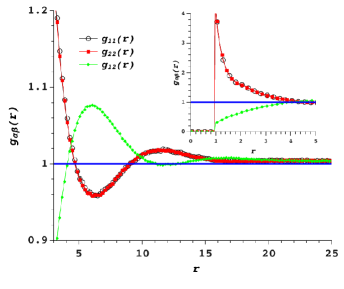
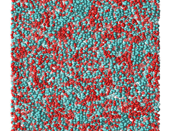
Figure 5: (Colour online) Pair distribution functions and a representative configuration for $T^{*}=0.28$, and volume fractions $\zeta_{1}=\zeta_{2}=0.026$.

We present the pair distribution functions, $g_{\alpha\beta}=\frac{G_{\alpha\beta}}{\zeta_{\alpha}\zeta_{\beta}}+1$, and representative configurations for $\zeta=0.052$ and $c=0$ in figures 5 and 6 for $T^{*}=0.28$, and $T^{*}=0.12$, respectively. In both cases, an oscillatory decay with the period of damped oscillations $\lambda\approx 10$ can be seen, but the amplitude is much larger for $T^{*}=0.12$. This larger amplitude and range of correlations is reflected in much more ordered configuration shown in figure 6, as compared with the configuration shown in figure 5. At $T^{*}=0.12$, we can see the chains of well assembled clusters, where clusters of different species are attached to each other. At $T^{*}=0.28$, the inhomogeneities are much less visible.

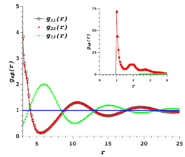
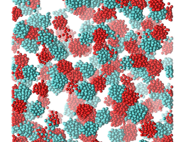
Figure 6: (Colour online) Pair distribution functions and a representative configuration for $T^{*}=0.12$, and volume fractions $\zeta_{1}=\zeta_{2}=0.026$.

We have computed $\tilde{G}_{\alpha\beta}$ for the thermodynamic states corresponding to figures 5 and 6. In the first case, we obtained a quite flat maximum of $\tilde{G}_{\alpha\alpha}(k)$. As far as a pronounced maximum is assumed in our theory and the theory should be self-consistent, for this thermodynamic state our theory is not accurate enough. In the second case, the maximum of $\tilde{G}_{\alpha\alpha}(k)$ is better developed, but the peak is not as high and narrow as for $\zeta=0.1$ at the same $T^{*}$. The corresponding pair distribution functions are shown in figure 7 for $r>8$, because in the mesoscopic theory the results for the correlation function cannot be valid for distances smaller than one period of the damped oscillations.

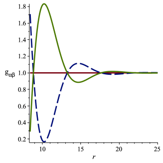
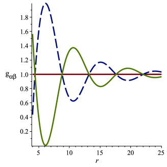
Figure 7: (Colour online) Left-hand panel: pair distribution functions in real space for $T^{*}=0.12$, $\zeta_{1}=\zeta_{2}=0.026$ with the effect of fluctuations taken into account in the mesoscopic theory. $g_{11}(r)=g_{22}(r)$ (solid line), and $g_{12}(r)$ (dashed line). Right-hand panel: Functions $g_{\alpha\beta}=G_{\alpha\beta}+1$, where $G_{\alpha\beta}$ is given in equation (1.1) with $\alpha_{1}=0.714$, $\alpha_{0}=0.1$, $\theta=0$ and $A=\pm 8.5$.

By comparing figure 7 with the simulation results (figure 6) we can see that in the theory the amplitude is too large and the decay length is too small. In figure 7 (right-hand panel) we plot $g_{\alpha\beta}=G_{\alpha\beta}+1$, where $G_{\alpha\beta}$ is given in (1.1) with $\alpha_{1}$ determined in our theory, but with $\alpha_{0}=0.1$ about 5 times smaller than predicted by the theory. The amplitude $A=8.5$ in equation (1.1) for $g_{11}(r)$ and $A=-8.5$ for $g_{12}(r)$ is also much smaller. We did not try to find the best fit to the simulation results, but it is clear that for the chosen parameters the agreement between simulations and equation (1.1) is very good. From this agreement, it immediately follows that in simulations the structure factor for the like (different) particles should assume a maximum (minimum) for $k\approx k_{0}$, and near the extremum it behaves as $|S_{\alpha\beta}|\propto[\text{const}+(k^{2}-k_{0}^{2})^{2}]^{-1}$. The theory developed in this work is based on the Brazovskii approximation. In  [31], additional correction to the MF inverse correlation function is taken into account. This correction term in one-component systems is proportional to $-A_{3}(\zeta)^{2}$, and leads to a smaller value of the inverse correlation function than in the Brazovskii approximation. Hence, larger correlations can be expected. A satisfactory agreement with the exact results was obtained in [31] for an equation of state in a one-dimensional model when the correction proportional to $-A_{3}(\zeta)^{2}$ was taken into account. Since $A_{3}(\zeta)=0$ for the critical volume fraction $\zeta\approx 0.129$, the Brazovskii approximation works well for $\zeta\approx 0.1$. $A_{3}(\zeta)$ increases to large values for $\zeta$ decreasing from $\zeta\approx 0.129$, and the accuracy of the Brazovskii approximation should decrease for a decreasing $\zeta$. Our results show that for $\zeta\approx 0.05$, the Brazovskii-type approximation is not sufficiently accurate. The period of damped oscillations, however, remains close to $2\piup/k_{0}$, and the formula (1.1) is still valid.

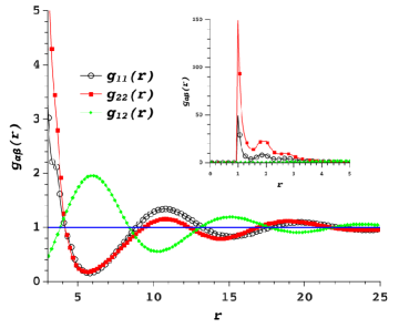
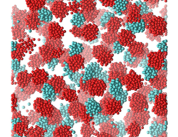
Figure 8: (Colour online) Pair distribution functions and a representative configuration for $T^{*}=0.12$, and volume fractions $\zeta_{1}=0.042$, $\zeta_{2}=0.01$.

The effect of asymmetry of the volume fractions of the two species is shown in figure 8 for $T^{*}=0.12$, $\zeta=0.052$ and $c=0.032$. Correlations between the majority species are stronger, in agreement with theoretical predictions. Clusters are of a similar size as in the symmetrical case. However, there are not enough particles of the minority component to fill the space between two clusters of the majority component, and this space remains empty. Recall that due to the long-range repulsion between the like particles, clusters of the same kind repel each other. For this reason, the correlation function for total volume fraction oscillates, in contrast to the symmetrical case. This result also agrees with theoretical predictions.

4 The case of interaction potentials $V_{11}=V_{22}=0$ and $V_{12}\neq 0$

Now, we consider a particular case of the model binary mixture in which there are only hard-core repulsions between the like-particles while the particles of different types interact through the attractive potential $V_{12}(r)$ beyond the hard core. The mixture can be perceived as a crude model of charged colloid particles in the solvent containing depletion agents. When charges are switched off, colloid particles attract each other due to the presence of depletants. If the particles are charged, screened electrostatic attraction between different particles appears, while the like-particles repel each other. For a suitably chosen size of the depletant and the screening length and charge, the attraction and repulsion between the like-particles can cancel each other approximately, and the attraction between the particles of different types can be doubled.

4.1 Theory

As the first step, we assume equal sizes of particles for all species. For $V_{12}(r)$, we choose the square well potential. Thus, the model is characterized by the following interaction potentials beyond the hard core

$$V_{11}(r) =V_{22}(r)=0,$$ (4.1)

$$V_{12}(r) =-\varepsilon\theta(r-1)\theta(a-r),$$ (4.2)

where $a>1$ is the range of the potential, $\varepsilon$ is the interaction strength at contact of the two unlike particles and $r$ is in $\sigma$ units. We are interested in periodic structure on the length scale of $\sigma$, not in any particular system. Since in [25] the MF phase diagram was obtained for $a=2$, we assume $a=2$ here too. The Fourier transform of the potential (4.2) for $a=2$ is shown in figure 10. The MF analysis showed [25] that the model undergoes two types of instability: one connected with $k=0$ and the other one with $k_{0}\approx 2.78$. The former is related to the gas-liquid phase separation which occurs at lower volume fractions while the latter is related to the appearance of local inhomogeneity at the length scale $2\piup/k_{0}$. In this model, inhomogeneous structures can occur when the Fourier transform of the interaction potential between unlike particles has positive maximum for $k>0$.

Figure 9: Interaction potential between particles of different kinds (equation (4.2) for $a=2$) in Fourier representation. The wave-number $k$ is in $\sigma^{-1}$ units.

Figure 10: Gas-liquid spinodals and $\lambda$-lines for the model (4.1)–(4.2) at $a=2$ for different $c^{*}=(\zeta_{1}-\zeta_{2})/\zeta$: $c^{*}=0$ (solid lines), $0.2$ (dashed lines), $0.4$ (dotted lines), $0.6$ (dash-dotted lines), and $0.8$ (short-dashed lines).

First, we focus on the MF approximation. In this case, the correlation functions in Fourier representation obtained for the model are of the form:

$$\tilde{G}_{11}^{\text{co}}(k)=\frac{A_{22}}{D^{\text{co}}(k)}\,,\quad\tilde{G}_{22}^{\text{co}}(k)=\frac{A_{11}}{D^{\text{co}}(k)}\,,\quad\tilde{G}_{12}^{\text{co}}(k)=-\frac{A_{12}+\beta\tilde{V}_{12}(k)}{D^{\text{co}}(k)}\,,$$ (4.3)

where $D^{\text{co}}(k)=A_{11}A_{22}-\left[A_{12}+\beta\tilde{V}_{12}(k)\right]^{2}$ and $\tilde{V}_{12}(k)$ is the Fourier transform of the interaction potential (4.2). From the equation $D^{\text{co}}(k)=0$ one can get the expressions for the gas-liquid spinodal and for the $\lambda$-surface, respectively

$$T_{\text{sp}}^{*}=\frac{\tilde{V}_{12}(0)}{\sqrt{A_{11}A_{22}}+A_{12}}\,,\qquad T_{\lambda}^{*}=\frac{\tilde{V}_{12}(k_{0})}{\sqrt{A_{11}A_{22}}-A_{12}}\,,$$ (4.4)

where the dimensionless temperature is defined as $T^{*}=k_{\text{B}}T/\varepsilon$. In figure 10, we present the $T^{*}$–$\zeta$-plots of the MF boundaries of stability determined by equations (4.4) for different values of $c^{*}=(\zeta_{1}-\zeta_{2})/\zeta$.

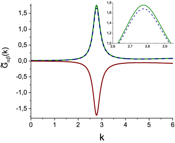
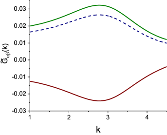
Figure 11: (Colour online) Correlation functions in Fourier representation for $T^{*}=2.5$, $\zeta=0.3$ and $c=0.06$ in MF approximation. The inset magnifies the region between $k=2.6$ and $k=3$ (left-hand panel) and with the effect of fluctuations taken into account (right-hand panel). Upper solid lines: $\tilde{G}_{11}(k)$, dashed lines: $\tilde{G}_{22}(k)$, and lower solid lines: $\tilde{G}_{12}(k)$.

Using equations (4.3), we calculate the MF correlation functions $\tilde{G}^{\text{co}}_{\alpha\beta}(k)$ above the $\lambda$-surface. Due to the proximity of the gas-liquid phase separation we chose the volume fraction equal to $0.3$ which is higher than in the case of the ‘two mermaids and a peacock’ model. As before, we assume that the majority component is the species 1, and consider only $c\geqslant 0$. The correlation functions $\tilde{G}^{\text{co}}_{\alpha\beta}(k)$ are shown in figure 11 (left-hand panel) for $T^{*}=2.5$ and $c=0.06$. The main maximum (minimum) of $\tilde{G}^{\text{co}}_{\alpha\beta}(k)$ corresponds to the maximum of the interaction potential $\tilde{V}_{12}$ (see figure 10). We observe a very small difference in the peak heights of $\tilde{G}^{\text{co}}_{11}(k)$ and $\tilde{G}^{\text{co}}_{22}(k)$ in this case.

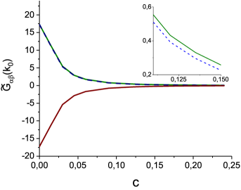
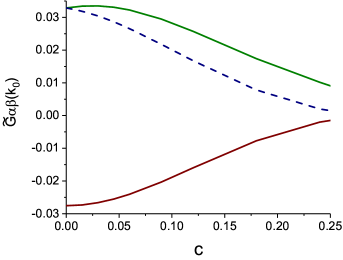
Figure 12: (Colour online) Left-hand panel: $\tilde{G}_{11}(k_{0})$ (upper solid line), $\tilde{G}_{22}(k_{0})$ (dashed line) and $\tilde{G}_{12}(k_{0})$ (lower solid line) in the MF approximation. The inset magnifies the region between $c=0.11$ and $c=0.15$. Right-hand panel: $\tilde{G}_{11}(k_{0})$ and $\tilde{G}_{22}(k_{0})$ with the effect of fluctuations taken into account. $T^{*}=2.5$, $\zeta=0.3$ and $c=\zeta_{1}-\zeta_{2}$.

In figure 12 (left-hand panel), we show the dependence of $\tilde{G}^{\text{co}}_{\alpha,\beta}(k_{0})$ on $c$. We see a monotonous dependence of the three correlation functions on $c$. At the same time, the difference in the peak heights of $\tilde{G}^{\text{co}}_{11}(k_{0})$ and $\tilde{G}^{\text{co}}_{22}(k_{0})$ increases a bit with an increase of $c$.

Now we consider the effect of fluctuations on the correlation functions. Like the ‘two mermaids and a peacock’ model considered in the previous section, $k_{0}$ in our model is not shifted when the fluctuations are included. For this model, $W^{\prime\prime}(k_{0})=-2\beta\tilde{V}_{12}^{\prime\prime}(k_{0})\tilde{C}_{12}(k_{0})$. As a result, equations (2.18) reduce to the form:

$$\tilde{C}_{\alpha\alpha}(k) =\tilde{C}_{\alpha\alpha}(k_{0}),\quad\alpha=1,2,$$

$$\tilde{C}_{12}(k) =\tilde{C}_{12}(k_{0})+\beta\Delta\tilde{V}_{12}(k),$$ (4.5)

where $\Delta\tilde{V}_{12}(k)=\tilde{V}_{12}(k)-\tilde{V}_{12}(k_{0})$. The correlation functions $\tilde{C}_{\alpha\beta}(k_{0})$ are obtained by solving equations (2.17). Finally, correlation functions $\tilde{G}_{\alpha\beta}(k)$ can be presented as follows:

$$\tilde{G}_{11}(k)=\frac{\tilde{C}_{22}(k_{0})}{D(k)}\,,\quad\tilde{G}_{22}(k)=\frac{\tilde{C}_{11}(k_{0})}{D(k)}\,,\quad\tilde{G}_{12}(k)=-\frac{\tilde{C}_{12}(k_{0})+\beta\Delta\tilde{V}_{12}(k)}{D(k)}\,,$$ (4.6)

where $D(k)=\tilde{C}_{11}(k_{0})\tilde{C}_{22}(k_{0})-[\tilde{C}_{12}(k_{0})+\beta\Delta\tilde{V}_{12}(k)]^{2}$. In the above equations, for $\Delta\tilde{V}_{12}(k)$ we use the approximation (3.6).

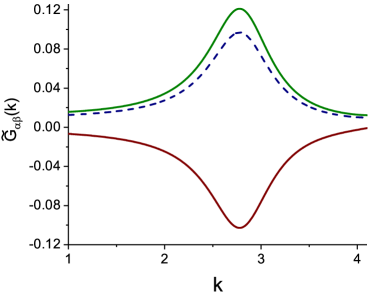
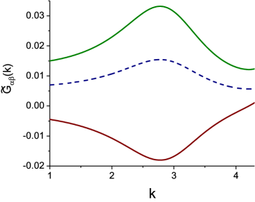
Figure 13: (Colour online) Correlation functions in Fourier representation for $T^{*}=0.8$ and $\zeta=0.3$ with the effect of fluctuations taken into account. Upper solid lines: $\tilde{G}_{11}(k)$, dashed lines: $\tilde{G}_{22}(k)$ and lower solid lines: $\tilde{G}_{12}(k)$. Left-hand panel: $c=0.06$. Right-hand panel: $c=0.18$.

Using equations (4.5)–(4.6) and taking into account (2.17), we calculate the correlation functions in Fourier representation for $\zeta=0.3$ and for the temperature above and below the $\lambda$-surface. In figure 11 (right-hand panel), $\tilde{G}_{\alpha\beta}(k)$ are compared with the MF result for the same values of the temperature, total volume fraction, and $c$. It is seen that the maxima (minimum) of the correlation functions for the temperature above the $\lambda$-surface become flat when the fluctuations are taken into account. We observe a nonmonotonous dependence of $\tilde{G}_{11}(k_{0})$ on $c$ with a maximum at $c\approx 0.03$ (see figure 12, right-hand panel) and this behaviour is kept above and below the $\lambda$-surface. The correlation functions $\tilde{G}_{22}(k_{0})$ and $\tilde{G}_{12}(k_{0})$ show a monotonous behaviour with an increasing $c$. In figure 13, we present $\tilde{G}_{\alpha\beta}(k)$ for $T^{*}=0.8$ and $c=0.06$ and $c=0.18$ (thermodynamic states below both the $\lambda$-surface and the gas-liquid spinodal). It is seen that the correlation functions have the same trend with an increase of $c$ as in the case of the ‘two mermaids and a peacock’ model: all correlations become weaker, especially the correlations between the particles of a minority component.

We should mention that the obtained extrema of the correlation functions in Fourier representation for $T^{*}=2.5$, $\zeta=0.3$ and $c=0.06$ as well as for $T^{*}=0.8$, $\zeta=0.3$ and $c=0.18$, are flat. However, we assumed that high, narrow peaks are present. Since the theory should be self-consistent, our findings signal that for these thermodynamic states our results cannot be accurate. For $T^{*}=0.8$, $\zeta=0.3$ and $c=0.06$, the extrema are more pronounced, and for this thermodynamic state better agreement with simulations can be expected.

In figure 14, the correlation functions in real space are presented. As is seen, $G_{\alpha\beta}(r)$ shows the qualitative behaviour similar to the behaviour of the corresponding correlation functions of the ‘two mermaids and a peacock’ model. The main difference is a period of oscillations which for this model is $\approx 2\sigma$.

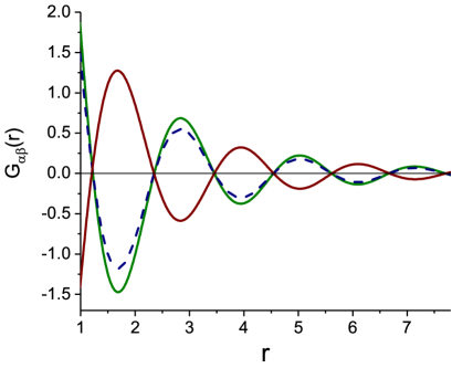
Figure 14: (Colour online) Correlation functions in real space for $T^{*}=0.8$, $\zeta=0.3$ and $c=0.06$ with the effect of fluctuations taken into account. $G_{11}(r)$ (green upper solid line on the left), $G_{22}(r)$ (dashed line) and $G_{12}(r)$ (red lower solid line on the left).

4.2 Simulations

A binary mixture of particles interacting with the potentials (4.1)–(4.2) was simulated using Monte Carlo technique in the $NVT$ ensemble. Particles ($N_{1}+N_{2}=15470$) are placed in a cubic box of the edge length $30\sigma$ with periodical boundary conditions in three directions. The volume fraction is $\zeta=0.3$. Particles of both species are of the same diameter ($\sigma_{1}=\sigma_{2}=\sigma=1.0$). A cut-off radius of $2\sigma$ is used, which is the interaction range of the square well potential. Each system has run $10^{6}$ Monte Carlo steps for equilibration and $10^{5}$ for production.

In figures 15–17, the pair distribution functions and representative configurations for $T^{*}=0.8$, $\zeta=0.3$ and for three values of $c$ are presented. The visualization suggests that for $c=0$ and $0.06$ the dilute gas phase coexists with the dense inhomogeneous liquid (figures 15–16). For the strongly asymmetric case ($c=0.18$), the dense inhomogeneous liquid with approximately equal densities of the two components coexists with the one-component, very dense gas (figure 17). In all cases, the inhomogeneous liquid phase mainly consists of stripes where the neighboring stripes are formed by the particles of different type. However, this picture is less pronounced for $c=0.18$.

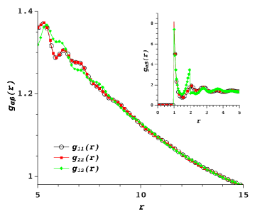
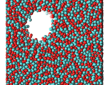
Figure 15: (Colour online) Pair distribution functions and a representative configuration for $T^{*}=0.8$, and volume fractions $\zeta_{1}=\zeta_{2}=0.15$ ($c=0$).

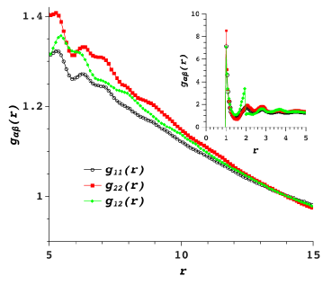
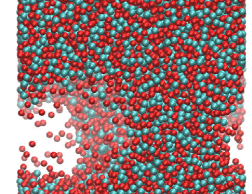
Figure 16: (Colour online) Pair distribution functions and a representative configuration for $T^{*}=0.8$, and volume fractions $\zeta_{1}=0.18$ and $\zeta_{2}=0.12$ ($c=0.06$).

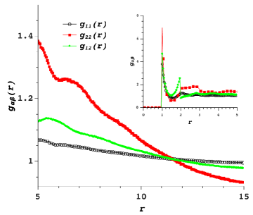
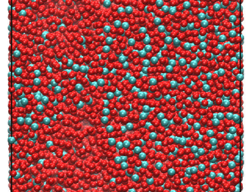
Figure 17: (Colour online) Pair distribution functions and a representative configuration for $T^{*}=0.8$, and volume fractions $\zeta_{1}=0.24$ and $\zeta_{2}=0.06$ ($c=0.18$).

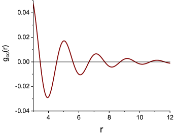
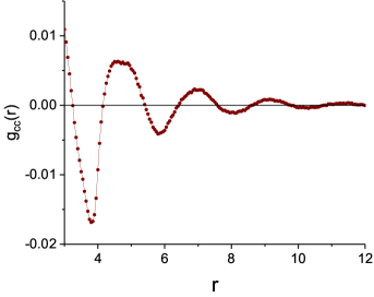
Figure 18: (Colour online) Concentration-concentration distribution function at $T^{*}=0.8$, $\zeta=0.3$ and $c=0.06$. Left-hand panel: theoretical results, right-hand panel: results of simulations.

It should be noted that the structure of the disordered inhomogeneous phase at $\zeta=0.3$ is affected by the packing of hard spheres. In order to separate the effect of hard-sphere packing we calculate the concentration-concentration distribution function $g_{cc}(r)=c_{1}^{2}c_{2}^{2}(g_{11}(r)+g_{22}(r)-2g_{12}(r))$, where $c_{i}=\zeta_{i}/\zeta$ [32]. The results are presented in figure 18. Here, we compare $g_{cc}(r)$ obtained from the theory (left-hand panel) and from the simulations (right-hand panel) for $T^{*}=0.8$, $\zeta=0.3$ and $c=0.06$. One can see a rather good agreement between the theoretical and simulation results: the distribution functions $g_{cc}(r)$ show an oscillatory decay around zero with the period of damped oscillations $\lambda\approx 2$, and the maxima and minima occur for very similar $r$ in theory and simulations. It is worth noting that in molten alkali halides, $g_{cc}(r)$ shows oscillations around zero, which extend over distances of at least 10 Å [33]. Since the simulation results for $g_{cc}(r)$ are well reproduced by equation (1.1), the corresponding structure factor takes a maximum for $k=k_{0}$, and the peak shape agrees with our predictions.

5 Conclusions

We have studied the effect of fluctuations on the correlation functions of a binary inhomogeneous mixture by using the mesoscopic density-functional theory. The theory is based on the Brazovskii-type approximation and allows one to take into account the fluctuation contribution. For a binary mixture in the disordered inhomogeneous phase, we have derived approximate equations for the partial correlation functions in Fourier representation. Using the above-mentioned approximations, we have calculated the correlation functions for several state points above and below the MF instability for two particular models of a binary mixture of species A and B. We have chosen models leading to a periodic structure on the length scale of the size of the particles, and on the length scale 10 times larger. We did so in order to compare the ordering and to verify the accuracy of the mesoscopic description for different length scales.

We have considered the two models in the MF and when the fluctuations are taken into account. In the two models, we have limited ourselves to an equal size of the hard cores of the particles of both species. In the first mixture, the particles of the same type interact with the ‘mermaid’ potential $V(r)$ (it has an attractive ‘head’ and a repulsive ‘tail’) while A and B particles interact with a ‘peacock’ potential $-V(r)$ which has an attractive ‘tail’ and a repulsive ‘head’. In the second mixture, there are only short-range attractive interactions between species A and B beyond the hard core which is chosen in the square-well form. In both models, the attractions lead to a periodic arrangement of alternating species A and B. However, the characteristic size of the regions rich in the particles of species A and B differ significantly in the two models. In addition, the gas-liquid phase separation can occur in the second model.

Despite different interaction potentials and different length scale of the local ordering, the correlation functions of the two models demonstrate similar properties. In order to verify the theoretical results and to visualize the structure for different state points, we have performed MC simulations. It is shown that the theoretical predictions are consistent with the simulation results.

Our results can be valid only for the case of well-defined inhomogeneities. Well developed short-range order occurs when the correlation functions in Fourier representation have high, narrow peaks at $k_{0}>0$. It is the case in the part of the phase diagram where the disordered phase looses stability in MF, but in reality it remains stable. Our theory agrees with simulations at a semiquantitative level for such state-points.

In the present paper, we have assumed equal size of the particles of different species. It is expected, however, that the periodic ordering should be enhanced when the size asymmetry increases. An increasing tendency for clustering with an increase of size asymmetry was observed in ionic systems in mesoscopic theory [25, 34] and in simulations [35, 36]. Further work is necessary for the study of the correlation functions in mixtures within the framework of the theory when the size asymmetry is taken into account.

Ukrainian 0

Âïëèâ ôëóêòóàöié íà êîðåëÿöiéíi ôóíêöi¿ ó íåîäíîðiäíèõ ñóìiøàõ À. Öÿõ${}^{\textsf{\footnotesize{\mbox{?}}}}$, Î. Ïàöàãàí${}^{\textsf{\footnotesize{\mbox{?}}}}$, À. Ìåéðà ${}^{\textsf{\footnotesize{\mbox{?},\penalty 1000\mbox{?}}}}$

             
${}^{\textsf{\footnotesize 1}}$ Iíñòèòóò ôiçèчíî¿ õiìi¿, Ïîëüñüêà àêàäåìiÿ íàóê, ì. Âàðøàâà, âóë. Êàñïøàêà, 44/32, Ïîëüùà ${}^{\textsf{\footnotesize 2}}$ Iíñòèòóò ôiçèêè êîíäåíñîâàíèõ ñèñòåì Íàöiîíàëüíî¿ àêàäåìi¿ íàóê Óêðà¿íè,
âóë. Ñâєíöiöüêîãî, 1, 79011 Ëüâiâ, Óêðà¿íà ${}^{\textsf{\footnotesize 3}}$ IFLYSIB (UNLP, CONICET), 59 No. 789, B1900BTE ì. Ëà-Ïëàòà, Àðãåíòèíà ${}^{\textsf{\footnotesize 4}}$ Íàöiîíàëüíèé òåõíîëîãiчíèé óíiâåðñèòåò - ðåãiîíàëüíèé ôàêóëüòåò Ëà-Ïëàòà, êàôåäðà ìàøèíîáóäóâàííÿ, ì. Ëà-Ïëàòà, Àðãåíòèíà

References

- [1] Leunissen M., Christova C., Hynninen A.P., Royal C., Campbell A., Imhof A., Dijkstra M., van Roji R., van Blaaderen A., Nature, 2005, 437, 235, doi:10.1038/nature03946.
- [2] Bartlett P., Campbell A.I., Phys. Rev. Lett., 2005, 95, No. 12, 128302, doi:10.1103/physrevlett.95.128302.
- [3] Shimizu K., Tariq M., Freitas A.A., Pádua A.A.H., Lopes J.N.C., J. Braz. Chem. Soc., 2015, 27, 349–362, doi:10.5935/0103-5053.20150274.
- [4] Hayes R., Warr G.G., Atkin R., Chem. Rev., 2015, 115, No. 13, 6357–6426, doi:10.1021/cr500411q.
- [5] Ciach A., Patsahan O., Phys. Rev. E, 2006, 74, 021508, doi:10.1103/PhysRevE.74.021508.
- [6] Patsahan O., Ciach A., J. Phys.: Condens. Matter, 2007, 19, 236203, doi:10.1088/0953-8984/19/23/236203.
- [7] Stradner A., Sedgwick H., Cardinaux F., Poon W., Egelhaaf S., Schurtenberger P., Nature, 2004, 432, 492, doi:10.1038/nature03109.
- [8] Campbell A.I., Anderson V.J., van Duijneveldt J.S., Bartlett P., Phys. Rev. Lett., 2005, 94, 208301, doi:10.1103/PhysRevLett.94.208301.
- [9] Sweatman M.B., Fartaria R., Lue L., J. Chem. Phys., 2014, 140, No. 12, 124508, doi:10.1063/1.4869109.
- [10] De Candia A., Gado E.D., Fierro A., Sator N., Tarzia M., Coniglio A., Phys. Rev. E, 2006, 74, 010403(R), doi:10.1103/PhysRevE.74.010403.
-
[11]
Santos A.P., Pȩkalski J., Panagiotopoulos A.Z., Soft Matter, 2017,
13, No. 44, 8055–8063,
doi:10.1039/C7SM01721A. - [12] Litniewski M., Ciach A., J. Chem. Phys., 2019, 150, 234702, doi:10.1063/1.5102157.
- [13] Royall C.P., Soft Matter, 2018, 14, 4020, doi:10.1039/c8sm00400e.
-
[14]
Bergman M., Garting T., Schurtenberger P., Stradner A., J. Phys. Chem. B, 2019,
123, 2432,
doi:10.1021/acs.jpcb.8b11781. - [15] Falus L.P., Fratini E., Chen W.R., Faraone A., Hong K., Baglioni P., Liu Y., J. Phys.: Condens. Matter, 2012, 24, 064114, doi:10.1088/0953-8984/24/6/064114.
- [16] Ciach A., Phys. Rev. E, 2008, 78, 061505, doi:10.1103/PhysRevE.78.061505.
- [17] Ciach A., Pękalski J., Góźdź W.T., Soft Matter, 2013, 9, 6301, doi:10.1039/C3SM50668A.
- [18] Edelmann M., Roth R., Phys. Rev. E, 2016, 93, 062146, doi:10.1103/PhysRevE.93.062146.
- [19] Pini D., Parola A., Soft Matter, 2017, 13, 9259, doi:10.1039/C7SM02125A.
-
[20]
Zhuang Y., Zhang K., Charbonneau P., Phys. Rev. Lett., 2016, 116,
098301,
doi:10.1103/PhysRevLett.116.098301. - [21] Brazovskii S.A., Sov. Phys. JETP, 1975, 41, 85.
- [22] Leibler L., Macromolecules, 1980, 13, 1602, doi:10.1021/ma60078a047.
- [23] Podneks V.E., Hamley I.W., JETP Lett., 1996, 64, 564, doi:10.1134/1.567271.
- [24] Ciach A., Soft Matter, 2018, 14, 5497, doi:10.1039/C8SM00602D.
- [25] Ciach A., Mol. Phys., 2011, 109, 1101, doi:10.1080/00268976.2010.548343.
- [26] Ciach A., J. Mol. Liq., 2018, 270, 138, doi:10.1016/j.molliq.2017.10.002.
- [27] Ciach A., Patsahan O., Condens. Matter Phys., 2012, 15, 23604, doi:10.5488/CMP.15.23604.
- [28] Otero-Mato J.M., Montes-Campos H., Cabeza O., Diddens D., Ciach A., Gallego L.J., Varela L.M., Phys. Chem. Chem. Phys., 2018, 20, 30412, doi:10.1039/C8CP05632C.
- [29] Ciach A., Adv. Biomembr. Lipid Self-Assembly, 2016, 23, 61, doi:10.1016/bs.abl.2015.12.004.
- [30] Ciach A., Góźdź W.T., Condens. Matter Phys., 2010, 13, 23603, doi:10.5488/CMP.13.23603.
- [31] Ciach A., Gozdz W.T., J. Phys.: Condens. Matter, 2016, 28, 414010, doi:10.1088/0953-8984/28/24/244004.
-
[32]
March N.H., Tosi M.P., Atomic Dynamics in Liquids, Macmillan Education, London, UK,
1976,
doi:10.1007/978-1-349-00929-9. - [33] March N.H., Tosi M.P., Introduction to Liquid State Physics, World Scientific Publishing, Singapore, 2002, doi:10.1142/4717.
- [34] Ciach A., Góźdź W.T., Stell G., Phys. Rev. E, 2007, 75, 051505, doi:10.1103/PhysRevE.75.051505.
- [35] Cheong D., Panagiotopoulos A., J. Chem. Phys., 2003, 119, 8526, doi:10.1063/1.1612473.
- [36] Spohr E., Hribar B., Vlachy V., J. Phys. Chem. B, 2002, 106, 2343, doi:10.1021/jp013811d.
Ukrainian \adddialect\l@ukrainian0 \l@ukrainian