Contribution of high risk groups’ unmet needs may be underestimated in epidemic models without risk turnover: a mechanistic modelling analysis

Abstract

Background. Epidemic models of sexually transmitted infections (STIs) are often used to characterize the contribution of risk groups to overall transmission by projecting the transmission population attributable fraction (tPAF) of unmet prevention and treatment needs within risk groups. However, evidence suggests that STI risk is dynamic over an individual’s sexual life course, which manifests as turnover between risk groups. We sought to examine the mechanisms by which turnover influences modelled projections of the tPAF of high risk groups. Methods. We developed a unifying, data-guided framework to simulate risk group turnover in deterministic, compartmental transmission models. We applied the framework to an illustrative model of an STI and examined the mechanisms by which risk group turnover influenced equilibrium prevalence across risk groups. We then fit a model with and without turnover to the same risk-stratified STI prevalence targets and compared the inferred level of risk heterogeneity and tPAF of the highest risk group projected by the two models. Results. The influence of turnover on group-specific prevalence was mediated by three main phenomena: movement of previously high risk individuals with the infection into lower risk groups; changes to herd immunity in the highest risk group; and changes in the number of partnerships where transmission can occur. Faster turnover led to a smaller ratio of STI prevalence between the highest and lowest risk groups. Compared to the fitted model without turnover, the fitted model with turnover inferred greater risk heterogeneity and consistently projected a larger tPAF of the highest risk group over time. Implications. If turnover is not captured in epidemic models, the projected contribution of high risk groups, and thus, the potential impact of prioritizing interventions to address their needs, could be underestimated. To aid the next generation of tPAF models, data collection efforts to parameterize risk group turnover should be prioritized.

Highlights

1. A new framework for parameterizing turnover in risk groups is developed

2. Mechanisms by which turnover influences STI prevalence in risk groups are examined

3. Turnover reduces the ratio of equilibrium STI prevalence in high vs low risk groups

4. Inferred risk heterogeneity is higher when fitting transmission models with turnover

5. Ignoring turnover in risk could underestimate the tPAF of high risk groups

Contents

1. 1 Introduction
2. 2 Methods
   1. 2.1 A unified framework for implementing turnover
   2. 2.2 Transmission model
   3. 2.3 Experiments
3. 3 Results
   1. 3.1 Experiment 1: Mechanisms by which turnover influences equilibrium prevalence
   2. 3.2 Experiment 2: Inferred risk heterogeneity with versus without turnover
      1. 3.3 Experiment 3: Influence of turnover on the tPAF of the high risk group
         1. 4 Discussion
            1. A Turnover Framework
               1. A.1 Notation
               2. A.2 Parameterization
               3. A.3 Previous Approaches
            2. B Supplemental Equations
               1. B.1 Model Equations
               2. B.2 Complete Example Turnover System
               3. B.3 Redundancy in specifying all elements of $\hat{e}$
               4. B.4 Factors of Incidence
            3. C Supplemental Results
               1. C.1 Equilibrium health states and rates of transition
      2. C.2 Equilibrium Prevalence Ratios
      3. C.3 Equilibrium Incidence
      4. C.4 Equilibrium prevalence and number of partners before and after model fitting
      5. C.5 Influence of turnover on the tPAF of the highest risk group before model fitting
         1. C.6 Effect of treatment rate on the influence of turnover on equilibrium prevalence

1 Introduction

Heterogeneity in transmission risk is a consistent characteristic of epidemics of sexually transmitted infections (STI) [2]. This heterogeneity is often demarcated by identifying specific populations whose risks of acquisition and onward transmission of STI are the highest, such that their specific unmet prevention and treatment needs can sustain local epidemics of STI [44]. Disproportionate risk can be conferred in several ways at the individual-level (higher number of sexual partners), partnership-level (reduced condom use within specific partnership types), or structural-level (stigma as a barrier to accessing prevention and treatment services) [4]. The contribution of high risk groups to the overall epidemic can then be used as an indicator in the appraisal of STI epidemics, helping to guide intervention priorities [39, 34].

Traditionally, contribution to an epidemic was quantified using either: the classic population attributable fraction (PAF) via the relative risk of incident infections within a risk group versus the rest of the population and the relative size of the risk group [17]; or the distribution of new infections across subsets of a population [8, 33]. So when small risk groups experience disproportionately higher rate of incident infections – e.g. 5 percent of a population acquire 30 percent of STI infections – contribution is interpreted as 5 percent of the population contributing to 30 percent of all infections [38]. However, the classic PAF does not account for chains of (indirect) transmission, and has been shown to underestimate the contribution of some higher-risk groups to cumulative STI infections, especially over time [33]. Thus, transmission models are increasingly being used to quantify contribution by accounting for indirect transmission and projecting the transmission population attributable fraction (tPAF). The tPAF is calculated by simulating counterfactual scenarios where transmission between specific subgroups is stopped, and the relative difference in cumulative infections in the total population over various time-periods is measured [33, 35]. Transmission can be stopped by setting susceptibility and/or infectiousness to zero in the model [33]. The tPAF is then interpreted as the fraction of all new infections that stem, directly and indirectly, from a failure to prevent acquisition and/or to provide effective treatment in a particular risk group [34, 35, 28].

There is limited evidence on how model structure might influence the tPAF of higher risk groups [34, 35, 28], especially movement of individuals between risk groups, an epidemiologic phenomenon that is well-described in the context of sexual behaviour [43]. Such movement is often referred to in the STI epidemiology literature as turnover [43]. For example, turnover may reflect entry into or retirement from formal sex work, or other periods associated with higher STI susceptibility and onward transmission due to more partners and/or vulnerabilities [30, 43]. Risk group turnover has been shown to influence the predicted equilibrium prevalence of an STI [40, 45]; the fraction of transmissions occurring during acute HIV infection [45]; the basic reproductive number $R_{0}$ [18]; and the coverage of antiretroviral therapy required to achieve HIV epidemic control [18]. Yet how, and the extent to which, turnover influences tPAF has yet to be examined.

There is variability in how turnover has been previously implemented [40, 23, 11, 7], in large part because of four main assumptions or epidemiologic constraints surrounding movement between risk groups. For example, in the context of turnover, the relative size of specific populations in the model may be constrained to remain constant over time [40, 23, 11], such as the proportion of individuals who sell sex. Second, some individuals may enter into high risk groups at an early age, and subsequently settle into lower risk groups; thus the distribution of risks among individuals entering into the transmission model may be assumed to be different from the distribution of risks among individuals already in the transmission model [11]. Third, turnover may be constrained to reflect the average duration of time spent within a given risk group [7], such as duration engaged in formal sex work [43]. Finally, turnover could reflect data on how sexual behaviour changes following exit from a given risk group [7]. Most prior models used some combination of these constraints, based on their specific data or research question, but to date there is no unified approach to modelling turnover.

In this study, we explored the mechanisms by which turnover may influence the tPAF of a high risk group using an illustrative STI model with treatment-induced immunity and without STI-attributable mortality. First, we developed a unified approach to implementing turnover based on epidemiologic constraints. We then sought the following objectives: 1) understand the mechanisms by which turnover influences group-specific STI prevalence and ratios of prevalence between risk groups; 2) examine how inclusion/exclusion of turnover in a model influences the level of risk heterogeneity inferred during model fitting; and 3) examine how inclusion/exclusion of turnover in a model influences the projected tPAF of the highest risk group after model fitting to a particular setting.

2 Methods

We developed a new, unified framework for implementing turnover. We then simulated a deterministic compartmental model of an illustrative STI, with turnover as per the framework, to conduct out experiments.

2.1 A unified framework for implementing turnover

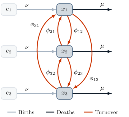
Figure 1: System of $G=3$ risk groups and turnover between them.

$x_{i}$: number of individuals in risk group $i$; $e_{i}$: number of individuals available to enter risk group $i$; $\nu$: rate of population entry; $\mu$: rate of population exit; $\phi_{ij}$: rate of turnover from group $i$ to group $j$.

We developed a framework for implementing turnover, as depicted in Figure 1 and detailed in Appendix A. In the framework, the simulated population is divided into $G$ risk groups. The number of individuals in group $i\in[1,\dots,G]$ is denoted $x_{i}$, and the relative size of each group is denoted $\hat{x}_{i}=x_{i}/N$, where $N$ is the total population size. Individuals enter the population at a rate $\nu$ and exit at a rate $\mu$ per year. The distribution of risk groups at entry into the model is denoted $\hat{e}_{i}$, which may be different from $\hat{x}_{i}$. The total number of individuals entering group $i$ per year is therefore given by $\nu\hat{e}_{i}N$. Turnover rates are collected in a $G\times G$ matrix $\phi$, where $\phi_{ij}$ is the proportion of individuals in group $i$ who move from group $i$ into group $j$ each year. The framework is independent of the disease model, and thus transition rates $\phi$ do not depend on health states.

The framework assumes that: 1) the relative sizes of risk groups $\bm{\hat{x}}=[\hat{x}_{1},\dots,\hat{x}_{G}]$ are known and should remain constant over time; and 2) the rates of population entry $\nu$ and exit $\mu$ are known, but that they may vary over time. An approach to estimate $\nu$ and $\mu$ is detailed in Appendix A.2.1. The framework then provides a method to estimate the values of the parameters $\bm{\hat{e}}$ and $\phi$, representing $G$ and $G(G-1)=G^{2}$ total unknowns. In the framework, $\bm{\hat{e}}$ and $\phi$ are collected in the vector $\bm{\theta}=\left[\bm{\hat{e}},\bm{y}\right]$, where $\bm{y}=\mathrm{vec}_{i\neq j}(\phi)$. To uniquely determine the elements of $\bm{\theta}$, a set of linear constraints are constructed. Each constraint $k$ takes the form $b_{k}=A_{k}\bm{\theta}$, where $b_{k}$ is a constant and $A_{k}$ is a vector with the same length as $\bm{\theta}$. The values of $\bm{\theta}$ are then obtained by solving:

$$\bm{b}=A\thinspace\bm{\theta}$$ (1)

using existing algorithms for solving linear systems [25].

The framework defines four types of constraints, which are based on assumptions, that can used to solve for the values of $\bm{\hat{e}}$ and $\phi$ via $\bm{\theta}$. The frameworks is flexible with respect to selecting and combining these constraints, guided by the availability of data. However, exactly $G^{2}$ non-redundant constraints must be specified to produce a unique solution, such that exactly one value of $\bm{\theta}$ satisfies all constraints. Table 1 summarizes the four types of constraints, with their underlying assumptions, and the types of data that can be used in each case. Additional details, including constraint equations, examples, and considerations for combining constraints, are in Appendix A.2.2.

Table 1: Summary of constraint types for defining risk group turnover

Constraint Assumption Parameters Types of data sources for parameterization 1. Constant group size the relative population sizes of groups are known or assumed, and assumed to not change over time $\hat{x}_{i}$ demographic health surveys [41], key population mapping and enumeration [1] 2. Specified elements the relative numbers of people entering into each group upon entry into the model or after leaving another group are known or assumed $\hat{e}_{i}$, $\phi_{ij}$ demographic health surveys [41], key population surveys [5] 3. Group duration the average durations of individuals in each group are known or assumed $\delta_{i}$ cohort studies of sexual behaviour over time [14], key population surveys [43, 5] 4. Turnover rate ratios ratios between different rates of turnover are known or assumed $\phi_{ij}$ demographic health surveys [41], key population surveys [5]

$\phi_{ij}$: rate of turnover from group $i$ to group $j$; $\hat{x}_{i}$: proportion of individuals in risk group $i$; $\hat{e}_{i}$: proportion of individuals entering into risk group $i$; $\delta_{i}$: average duration spent in risk group $i$.

2.2 Transmission model

We developed a deterministic, compartmental model of an illustrative sexually transmitted infection with 3 risk groups. We did not simulate a specific pathogen, but rather constructed a biological system that included susceptible, infectious, and treated (or recovered/immune) health states. The transmission model therefore was mechanistically representative of sexually transmitted infections like HIV, where effective antiretroviral treatment represents a health state where individuals are no longer susceptible nor infectious [27], or hepatitis B virus, where a large proportion of individuals who clear their acute infection develop life-long protective immunity [15].

The model is represented by a set of coupled ordinary differential equations (Appendix B.1) and includes three health states: susceptible $\mathcal{S}$, infectious $\mathcal{I}$, and treated $\mathcal{T}$ (Figure 2), and $G=3$ levels of risk: high $H$, medium $M$, and low $L$.

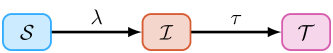
Figure 2: Modelled health states: $\mathcal{S}$: susceptible; $\mathcal{I}$: infected; $\mathcal{T}$: treated; and transitions: $\lambda$: force of infection; $\tau$: treatment.

Risk strata are defined by different number of partners per year, so that individuals in risk group $i$ are assumed to form partnerships at a rate $C_{i}$ per year. The probability of partnership formation $\rho_{ik}$ between individuals in group $i$ and individuals in risk group $k$ is assumed to be proportionate to the total number of available partnerships within each group [16]:

$$\rho_{ik}=\frac{C_{k}x_{k}}{\sum_{\mathrm{k}}C_{\mathrm{k}}x_{\mathrm{k}}}$$ (2)

The biological probability of transmission is defined as $\beta$ per partnership. Individuals transition from the susceptible $\mathcal{S}$ to infectious $\mathcal{I}$ health state via a force of infection $\lambda_{i}$ per year, per susceptible in risk group $i$:

$$\lambda_{i}=C_{i}\sum_{k}\rho_{ik}\thinspace\beta\thinspace\frac{\mathcal{I}_{k}}{x_{k}}$$ (3)

Individuals are assumed to transition from the infectious $\mathcal{I}$ to treated $\mathcal{T}$ health state at a rate $\tau$ per year, reflecting diagnosis and treatment. The treatment rate does not vary by risk group. Individuals in the treated $\mathcal{T}$ health state are neither infectious nor susceptible, and individuals cannot become re-infected.

2.2.1 Implementing turnover within the transmission model

As described in Section 2.1, individuals enter the model at a rate $\nu$, exit the model at a rate $\mu$, and transition from risk group $i$ to group $j$ at a rate $\phi_{ij}$, health state. The turnover rates $\phi$ and distribution of individuals entering the model by risk group $\bm{\hat{e}}$ were computed using the methods outlined in Appendix A.2.2, based on the following three assumptions. First, we assumed that the proportion of individuals entering each risk group $\bm{\hat{e}}$ was equal to the proportion of individuals across risk groups in the model $\bm{\hat{x}}$. Second, we assumed that the average duration of time spent in each risk group $\bm{\delta}$ was known. Third, we assumed that the absolute number of individuals moving between two risk groups in either direction was balanced, meaning that if 10 individuals moved from group $i$ to group $j$, then another 10 individuals moved from group $j$ to group $i$. These three assumptions were selected because they reflect the common assumptions underlying turnover in prior models [45, 18] and also to avoid any dominant direction of turnover. That is, we wanted to study the influence of movement between risk groups in general, as compared to no movement, and at various rates of movement, rather than movement predominantly from some groups to some other groups. The system of equations formulated from the above assumptions and constraints is given in Appendix B.2. To satisfy all three assumptions, there was only one possible value for each element in $\phi$ and $\bm{\hat{e}}$. That is, by specifying these three assumptions, we generated a unique set of $\phi$ and $\bm{\hat{e}}$.

Under the above three assumptions, we still needed to specify the particular values of the parameters $\bm{\hat{x}}$, $\bm{\delta}$, $\nu$, and $\mu$. Such parameter values could be derived from data as described in Appendix A.2.2. However, in all our experiments, we used the illustrative values summarized in Table 2. After resolving the system of equations Eq. (1) using these values, $\bm{\hat{e}}$ was equal to $\bm{\hat{x}}$ (assumed), and $\phi$ was:

$$\phi=\left[\begin{array}[]{ccc}*&0.0833&0.0867\\ 0.0208&*&0.0158\\ 0.0058&0.0042&*\end{array}\right]$$ (4)

Table 2: Default model parameters for experiments

Symbol Description Default value $\bm{\beta}$ transmission probability per partnership $0.03$ $\tau$ rate of treatment initiation among infected $0.1$ $N_{0}$ initial population size $1000$ $\bm{\hat{x}}$ proportion of system individuals by risk group $[0.05\enspace 0.20\enspace 0.75]$ $\bm{\hat{e}}$ proportion of entering individuals risk by risk group $[0.05\enspace 0.20\enspace 0.75]$ $\bm{\delta}$ average duration spent in each risk group $[5\enspace 15\enspace 25]$ $C$ number of partners per year by individuals in each risk group $[25\enspace 5\enspace 1]$ $\nu$ rate of population entry $0.05$ $\mu$ rate of population exit $0.03$

All rates have units $\mathrm{year}^{-1}$; durations are in $\mathrm{years}$; parameters stratified by risk group are written [high, medium, low] risk.

We then simulated epidemics using $\phi$ above and the parameters shown in Table 2. The transmission model was initialized with $N_{0}=1000$ individuals who were distributed across risk groups according to $\bm{\hat{x}}$. We seeded the epidemic with one infectious individual in each risk group at $t=0$ in an otherwise fully susceptible populatuon. We numerically solved the system of ordinary differential equations (Appendix B.1) in Python using Euler’s method with a time step of $dt=0.1$ years. Code for all aspects of the project is available at: https://github.com/mishra-lab/turnover.

2.3 Experiments

We designed three experiments to examine the influence of turnover on simulated epidemics. We analyzed all outcomes at equilibrium, defined as steady state at $t=500$ years with $<1\%$ change in incidence per year.

2.3.1 Experiment 1: Mechanisms by which turnover influences equilibrium prevalence

We designed Experiment 1 to explore the mechanisms by which turnover influences the equilibrium STI prevalence of infection, and the ratio of prevalence between risk groups (prevalence ratios). We defined prevalence as $\hat{\mathcal{I}}_{i}=\dfrac{\mathcal{I}_{i}}{x_{i}}$. Similar to previous studies [45, 18], we varied the rates of turnover using a single parameter. However, because our model had $G=3$ risk groups, multiplying a set of base rates $\phi$ by a scalar factor would change the relative population sizes of risk groups $\bm{\hat{x}}$. Instead of a scalar factor, we controlled the rates of turnover using the duration of time spent in the high risk group $\delta_{H}$, because of the practical interpretation of $\delta_{H}$ in the context of STI transmission, such as the duration in formal sex work [43]. A shorter $\delta_{H}$ yielded faster rates of turnover among all groups. The duration of time spent in the medium risk group $\delta_{M}$ was then defined as a value between $\delta_{H}$ and the maximum duration $\mu^{-1}$ which scaled with $\delta_{H}$ following: $\delta_{M}=\delta_{H}+\kappa\left(\mu^{-1}-\delta_{H}\right)$, with $\kappa=0.3$. The duration of time in the low risk group $\delta_{L}$ similarly scaled with $\delta_{H}$, but due to existing constraints, specification of $\delta_{H}$ and $\delta_{M}$ ensured only one possible value of $\delta_{L}$. Thus, each value of $\delta_{H}$ yielded a unique set of turnover rates $\phi$ whose elements all scaled inversely with the duration in the high risk group $\delta_{H}$.

We varied $\delta_{H}$ across a range of 33 to 3 years, reflecting a range from the full duration of simulated sexual activity $\mu^{-1}\approx 33$ years, through an average reported duration in sex work as low as 3 years [43]. The resulting duration of time spent in each group versus turnover in the high risk group $\delta_{H}^{-1}$ is shown in Figure 3.

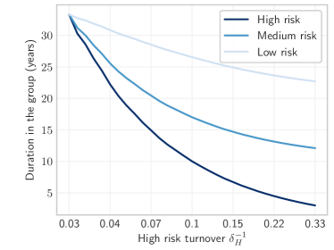
Figure 3: Average duration of time spent in each risk group versus turnover.

Turnover rate (log scale) is a function of the duration of time spent in the high risk group $\delta_{H}$, where shorter time spent in the high risk group yields faster turnover. No turnover is indicated by $\delta_{H}^{-1}=0.03$, due to population exit rate $\mu=0.03$.

For each set of turnover rates, we plotted the equilibrium prevalence in each risk group, and the prevalence ratios between high/low, high/medium, and medium/low risk groups. In order to understand the mechanisms by which turnover influenced prevalence and prevalence ratios (Objective 1), we additionally plotted the four components which contributed to gain/loss of infectious individuals in each risk group, based on Eq. (B.1b): 1) net gain/loss via turnover of infectious individuals, 2) gain via incident infections, 3) loss via treatment, and 4) loss via death. The influence of turnover on prevalence was only mediated by components 1 and 2, since components 3 and 4 were defined as constant rates which did not change with turnover; as such, our analysis focused on components 1 and 2. Finally, to further understand trends in incident infections versus turnover (component 1), we factored equation Eq. (3) for incidence $\lambda_{i}$ into constant and non-constant factors, and plotted the non-constant factors versus turnover.

2.3.2 Experiment 2: Inferred risk heterogeneity with vs without turnover

We designed Experiment 2 to examine how the inclusion versus exclusion of turnover influences the inference of transmission model parameters related to risk heterogeneity, specifically the numbers of partners per year $C_{i}$ across risk groups. The ratio of partner numbers $C_{H}~{}/~{}C_{L}$ is one way to measure of how different the two risk groups are with respect to acquisition and transmission risks. Indeed, ratios of partner numbers are often used when parameterizing risk heterogeneity in STI transmission models [32].

First, we fit the transmission model with turnover and without turnover, to equilibrium infection prevalence across risk groups. Specifically, we held all other parameters at their default values and fit the numbers of partners per year in each risk group $C_{i}$ to reproduce the following: 20% infection prevalence among the high risk group, 8.75% among the medium risk group, 3% among the low risk group, and 5% overall. To identify the set of parameters (i.e. partner numbers $C$ in each risk group) that best reproduced the fitting targets, we minimized the negative log-likelihood of group-specific and overall prevalence. Sample sizes of 500, 2000, 7500, and 10,000 were assumed to generate binomial distributions for the high, medium, low, and overall prevalence targets respectively, reflecting typical sample sizes in nationally representative demographic and health surveys [41], multiplied by the relative sizes of risk groups in the model $\bm{\hat{x}}$. The minimization was performed using the SLSQP method [24] from the SciPy Python minimize package. To address Objective 2, we compared the fitted (posterior) ratio of partners per year $C_{H}~{}/~{}C_{L}$ in the model with turnover versus the model without turnover.

2.3.3 Experiment 3: Influence of turnover on the tPAF of the high risk group

We designed Experiment 3 to examine how the tPAF of the high risk group varies when projected by a model with versus without turnover (Objective 3). We calculated the tPAF of risk group $i$ by comparing the relative difference in cumulative incidence between a base scenario, and a counterfactual where transmission from group $i$ is turned off, starting at the fitted equilibrium. That is, in the counterfactual scenario, infected individuals in the high risk group could not transmit the infection. The tPAF was calculated over different time-horizons (1 to 50 years) as [33]:

$$\textrm{tPAF}_{i}(t)=\frac{\displaystyle\int_{t_{eq}}^{t}I_{b}(\tau)\,d\tau-\displaystyle\int_{t_{eq}}^{t}I_{c}(\tau)\,d\tau}{\displaystyle\int_{t_{eq}}^{t}I_{b}(\tau)\,d\tau}$$ (5)

where $t_{eq}$ is the time corresponding to equilibrium, $I_{b}(t)$ is the rate of new infections at time $t$ in the base scenario, and $I_{c}(t)$ is the rate of new infections at time $t$ in the counterfactual scenario. We then compared the tPAF generated from the fitted model with turnover to the tPAF generated from the fitted model without turnover.

3 Results

3.1 Experiment 1: Mechanisms by which turnover influences equilibrium prevalence

Figure 4 shows the trends in equilibrium STI prevalence among the high (4(a)), medium (4(b)), and low (4(c)) risk groups, at different rates of turnover which are depicted on the x-axis, based on duration of time spent in the high risk group. Figure 4 reveals an inverted U-shaped relationship between STI prevalence and turnover in all three risk groups. That is, equilibrium STI prevalence was higher in systems with slow turnover versus those with no turnover (Figure 4, region A). Equilibrium STI prevalence then peaked at slightly faster turnover before declining in systems with even faster turnover (region B in Figure 4). Comparison of group-specific prevalence in Figure 4 shows that the threshold turnover rate at which group-specific prevalence peaked varied by risk group: prevalence in the high risk group peaked at the lower turnover threshold (Figure 4(a)), while prevalence in low risk group peaked at a higher turnover threshold (Figure 4(c)). To explain the inverted U-shape and different turnover thresholds by group, we examined the components contributing to prevalence, first in the high risk group, and then in the low risk group.

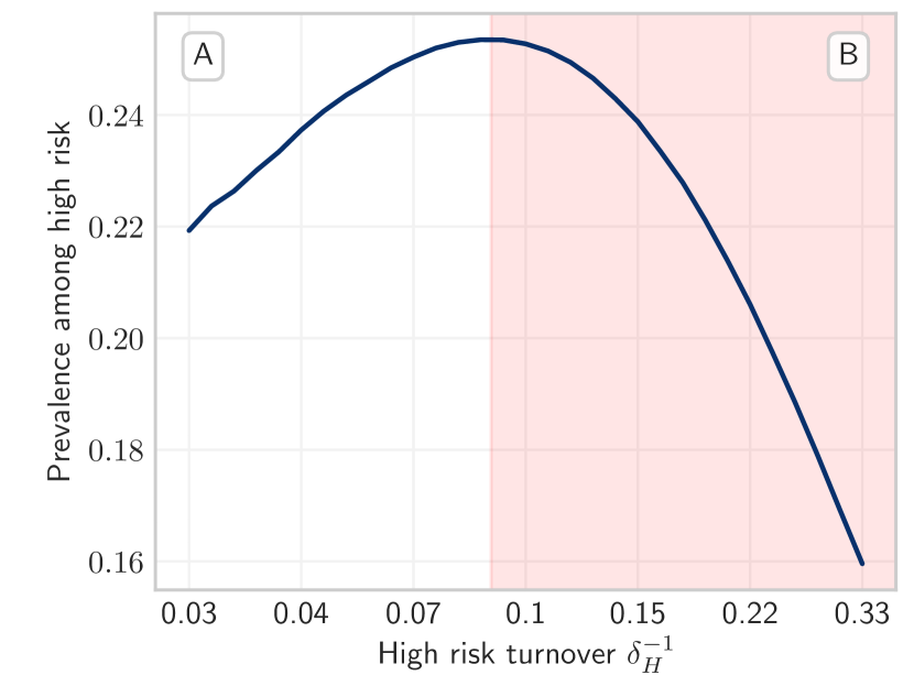
(a) High risk

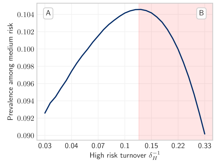
(b) Medium risk

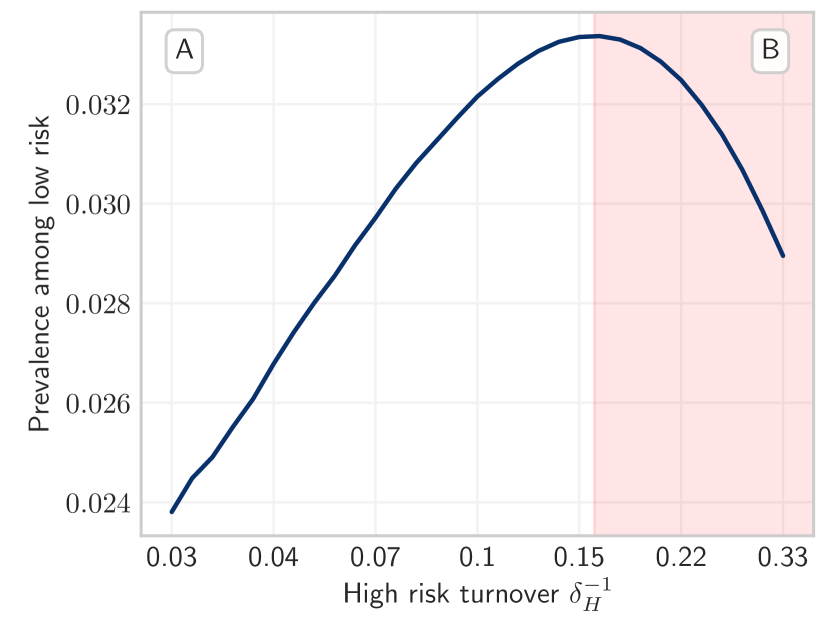
(c) Low risk

Figure 4: Relationship between equilibrium STI prevalence in high, medium, and low risk groups versus turnover rate. Regions A and B denote where equilibrium prevalence is increasing and decreasing with different rates of turnover, respectively.

Turnover rate (log scale) is a function of the duration of time spent in the high risk group $\delta_{H}$, where shorter time spent in the high risk group yields faster turnover. No turnover is indicated by $\delta_{H}^{-1}=0.03$, due to population exit rate $\mu=0.03$.

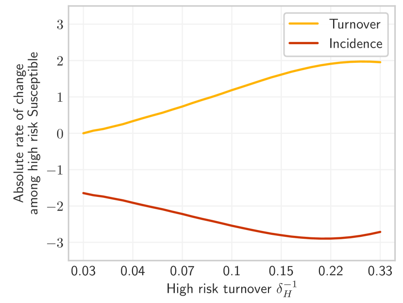
(a) High risk susceptible

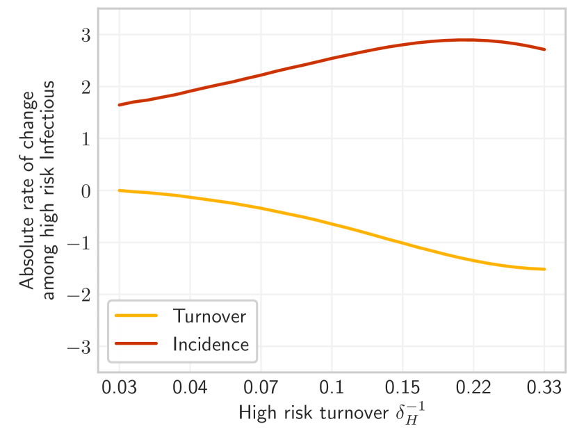
(b) High risk infectious

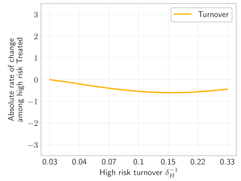
(c) High risk treated

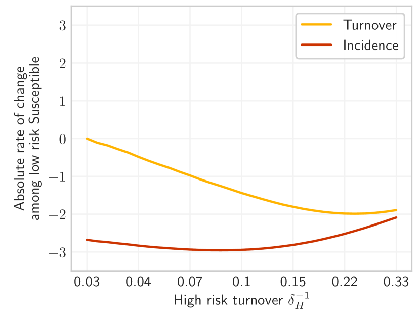
(d) Low risk susceptible

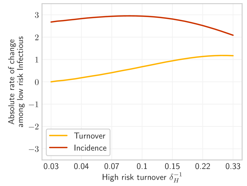
(e) Low risk infectious

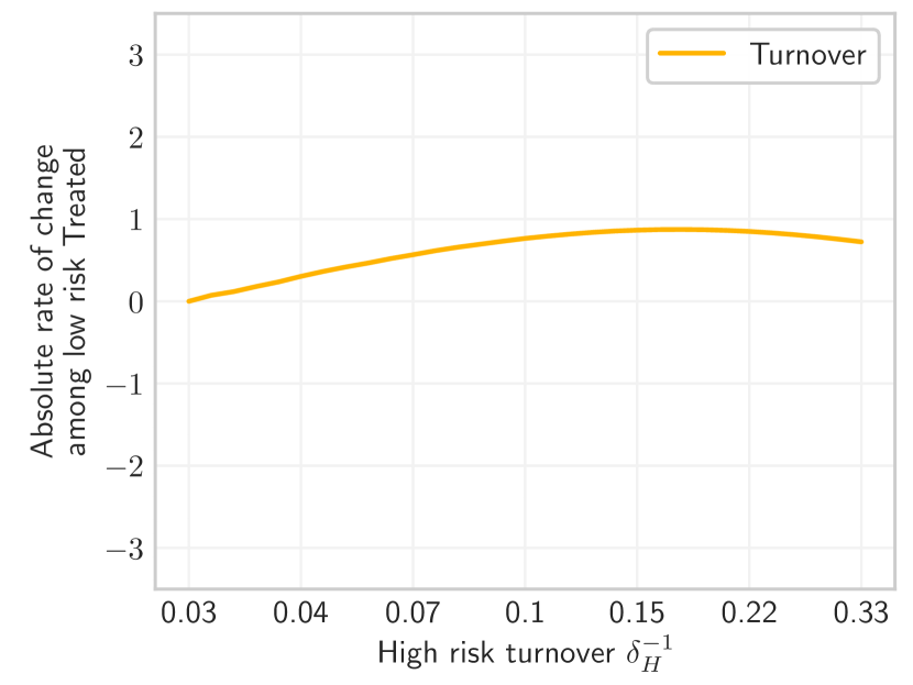
(f) Low risk treated

Figure 5: Absolute rates of change at equilibrium (number of individuals gained/lost per year) among individuals in each health state and risk group, due to: loss/gain via turnover (yellow), and loss/gain via incident infections (red). Based on Eq. (B.1). See Figure 3.2 for all derivative components.

Turnover rate (log scale) is a function of the duration of time spent in the high risk group $\delta_{H}$, where shorter time spent in the high risk group yields faster turnover. No turnover is indicated by $\delta_{H}^{-1}=0.03$, due to population exit rate $\mu=0.03$.

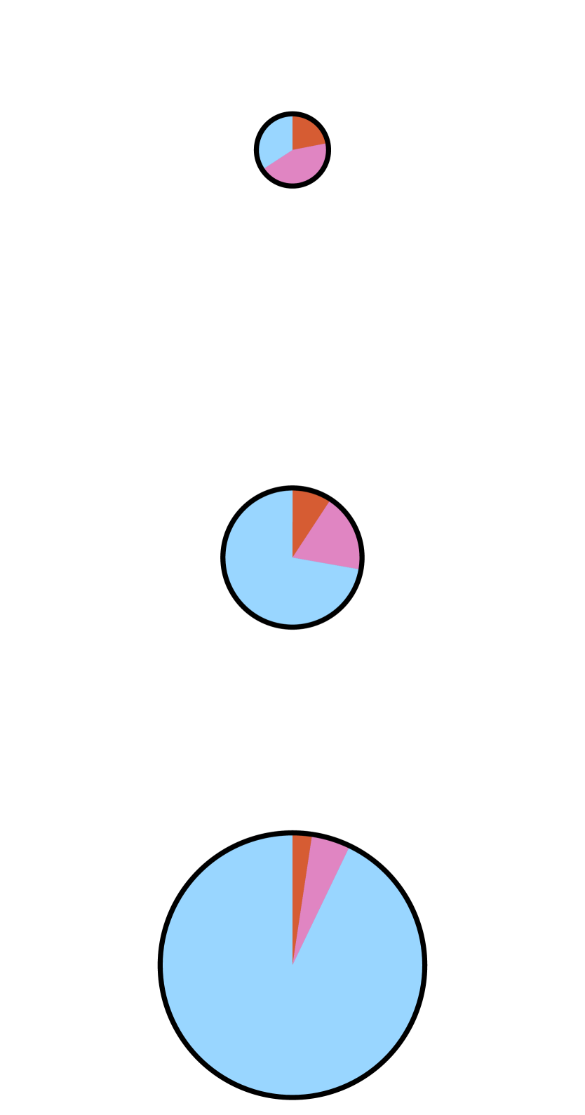
(a) No turnover

$\delta_{H}^{-1}=0.03$

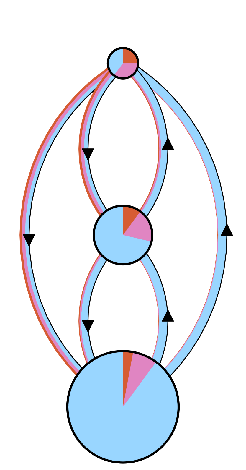
(b) Slow turnover

$\delta_{H}^{-1}=0.062$

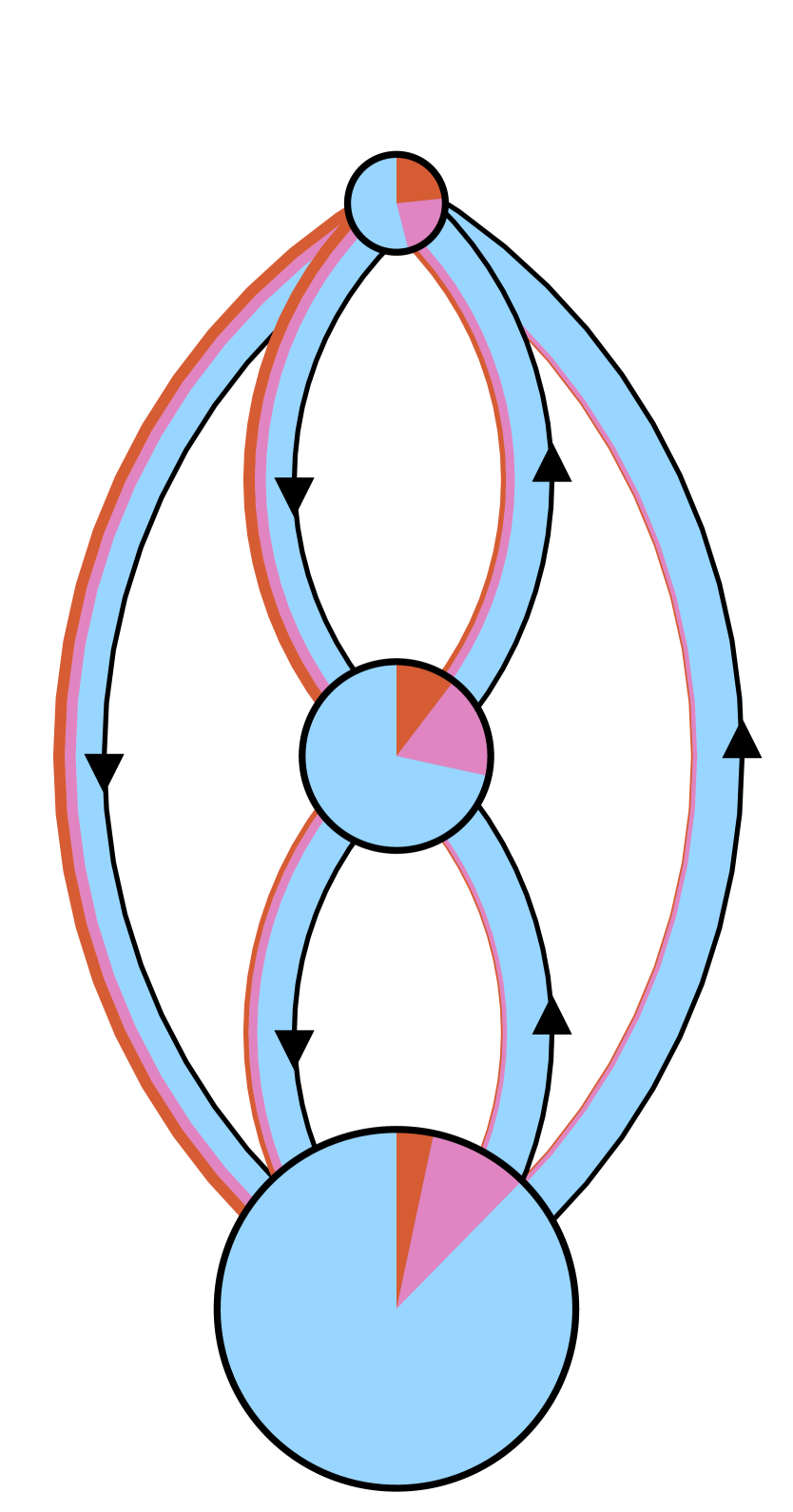
(c) Fast turnover

$\delta_{H}^{-1}=0.162$

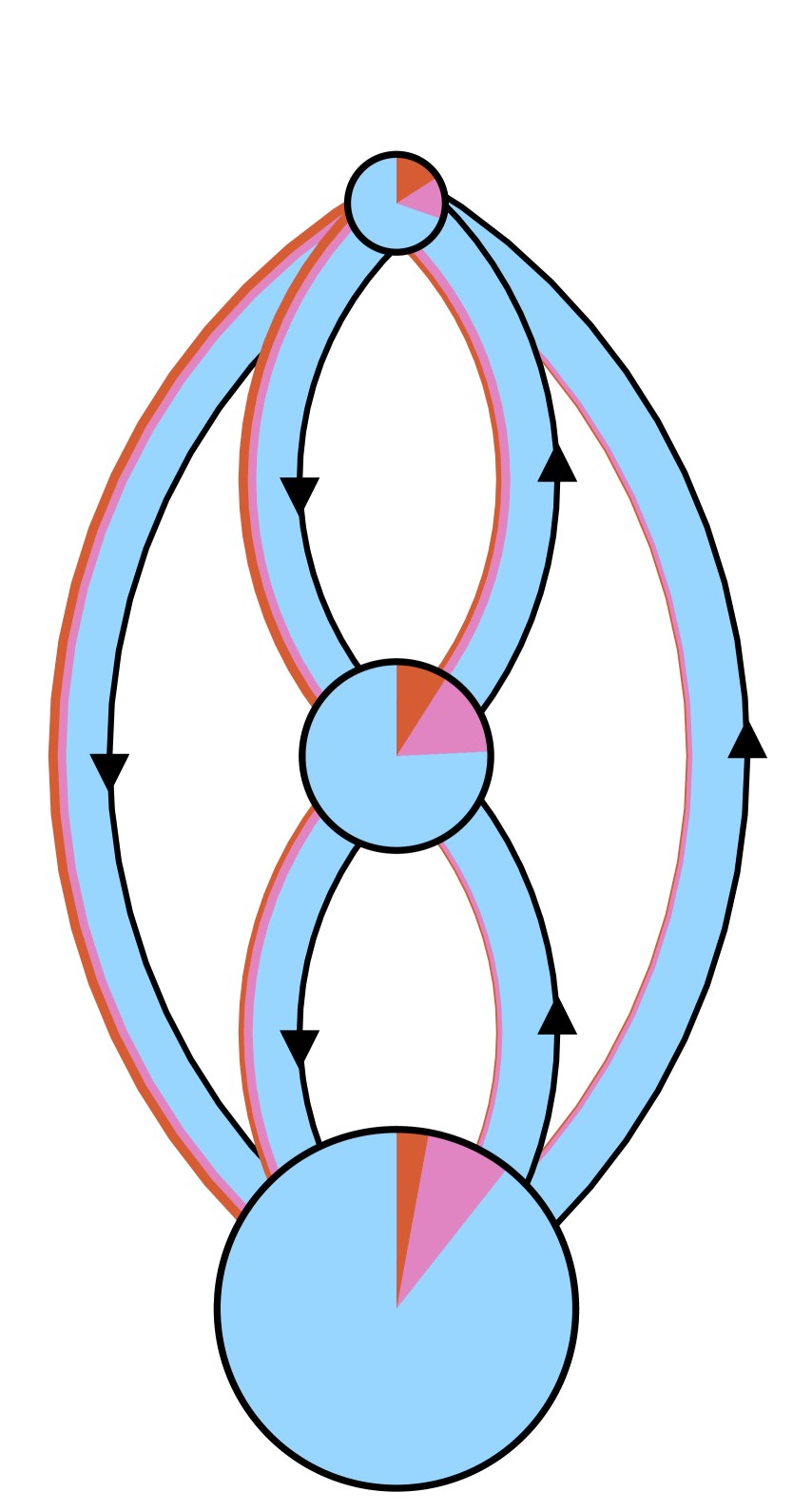
(d) Very fast turnover

$\delta_{H}^{-1}=0.333$

Figure 6: Depiction of health states of individuals in each risk group and of individuals moving between risk groups, obtained from models at equilibrium under four overall rates of turnover.

$\hbox{}\hskip 47.69846pt\underbrace{\hskip 190.79385pt}_{\textrm{Region~{}A}}\underbrace{\hskip 190.79385pt}_{\textrm{Region~{}B}}$ Circle sizes are proportional to risk group sizes. Circle slices and arrow widths are also proportional to the proportion of health states within risk groups and among individuals moving between risk groups, respectively. However, circle sizes and arrow widths do not have comparable scales. Appendix Figure 3.2 illustrates proportions of health states versus turnover in full.

Figure 5 shows the yearly gain/loss of individuals via turnover, and gain/loss via incident infections, in each health state and risk group, at equilibrium under different rates of turnover. Figure 6 also illustrates the distribution of health states in each risk group and among individuals moving between risk groups under four different rates of turnover.

3.1.1 Influence of turnover on equilibrium prevalence in the high risk group

As shown in Figure 6, at all four rates of turnover the proportion of individuals who were in the infectious state (STI prevalence) was largest in the high risk group. As infectious individuals left the high risk group via turnover, they were largely replaced by susceptible individuals from lower risk groups (Figure 6(b) and Figures 5(a) vs 5(b), yellow). The pattern of net outflow of infectious individuals from the high risk group via turnover persisted across the range of turnover rates (Figure 5(b), yellow). This net outflow of infectious individuals via turnover acted to reduce STI prevalence in the high risk group (phenomenon 1). Treated individuals were similarly replaced largely by susceptible individuals (Figure 6(b) and Figures 5(a) vs 5(c), yellow). The net replacement of both infectious and treated individuals with susceptible individuals in the high risk group acted to reduce herd immunity in that group. Reduced herd immunity then contributed to a rise in the number of incident infections in the high risk group, as the system moved from no turnover to slow turnover (Figure 5(b), red; phenomenon 2). Incidence was further influenced by a third phenomenon as systems moved from no turnover to higher rates of turnover: the net movement of infectious individuals from high to low risk (Figure 6(b)) reduced the average number of partners per year made available by individuals in the infectious state (Figure 7(a)). As shown in Appendix B.4, modelled incidence in all risk groups was proportional to the average number of partners per year among infectious individuals (Figure 7(a)), and overall prevalence (Figure 7(b)). Thus, as the average number of partners per year among infectious individuals fell with faster turnover, incidence decreased (Figure 7(c), region B; phenomenon 3).

Therefore, the inverted U-shaped relationship between turnover rate and equilibrium STI prevalence in the high risk group was mediated by the combination of the above three phenomena. When systems moved from no turnover to slow turnover, reduction in herd immunity (phenomenon 2) predominated, leading to increasing equilibrium prevalence with turnover (Figure 4(a), region A). When systems were modelled under faster and faster turnover, outflow of infectious individuals from the group via turnover (phenomenon 1) and reduction in the average number of partners per year among infectious individuals (phenomenon 3) predominated, leading to lower equilibrium prevalence at faster rates of turnover (Figure 4(a), region B).

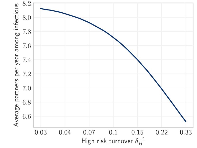
(a) Average number of partners per year among infectious individuals

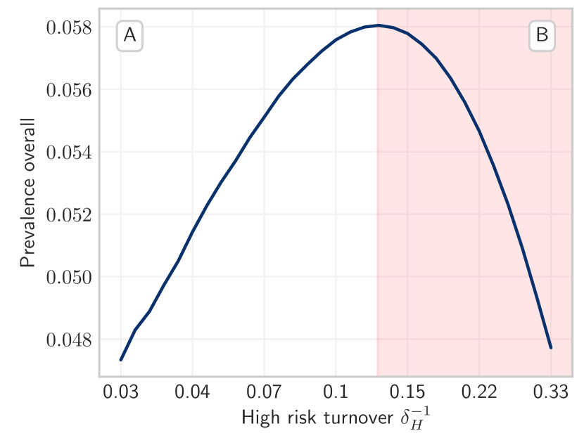
(b) Overall prevalence

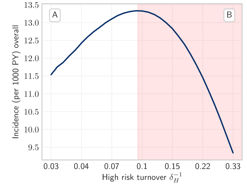
(c) Overall incidence

Figure 7: Overall incidence and the non-constant factors of incidence versus turnover. The product of factors (7(a)) and (7(b)) is proportional to (7(c)) overall incidence. See Appendix B.4 for proof.

Turnover rate (log scale) is a function of the duration of time spent in the high risk group $\delta_{H}$, where shorter time spent in the high risk group yields faster turnover. No turnover is indicated by $\delta_{H}^{-1}=0.03$, due to population exit rate $\mu=0.03$.

3.1.2 Influence of turnover on equilibrium prevalence in the low risk group

As shown in Figure 6, at equilibrium, the low risk group was composed mainly of susceptible individuals. Moving from a system no turnover to one with slow turnover lead to a net inflow of infectious and treated individuals (Figures 5(e) and 5(f), yellow), and a net removal of susceptible individuals (Figure 5(d), yellow). The net inflow of infectious individuals (Figure 5(e), yellow) contributed to higher equilibrium prevalence in the low risk group when the system moved from no turnover to slow turnover (phenomenon 1). The inflow of infectious and treated individuals only slightly reduced the already large proportion who were susceptible in the low risk group. Thus, there was little increase in herd immunity within the low risk group as turnover increased (phenomenon 2). However, incident infections still rose in the low risk group as the system moved from no turnover to slow turnover (Figure 5(e), red) due to higher incidence in the total population (Figure 7(c)) which was largely driven by reduced herd immunity in the high risk group (see Section 3.1.1; phenomenon 2). Under faster rates of turnover, incident infections declined in the low risk group (Figure 5(e), red) due to lower incidence in the total population (Figure 7(c)) which was driven by decreasing number of partners per year among infectious individuals (Figure 7(a); phenomenon 3), as described in Section 3.1.1.

Therefore, as in the high risk group, the inverted U-shaped relationship between turnover rate and equilibrium STI prevalence in the low risk group was mediated by the combination of the above three phenomena. Moving from no turnover to slow turnover, the net inflow of infectious individuals (phenomenon 1) and reduced herd immunity in the high risk group (phenomenon 2) predominated, leading to higher equilibrium prevalence (Figure 4(c), region A). At higher rates of turnover, a decreasing overall incidence due to a reduction in the number of partners among infectious individuals (phenomenon 3) predominated, leading to declining equilibrium prevalence (Figure 4(c), region B).

In sum, there were three phenomena that drove shifts in equilibrium STI prevalence across risk groups at variable rates of turnover: 1) net flows of infectious individuals from high risk groups into low risk groups; 2) changes to herd immunity, especially within the high risk group; and 3) changes to the number of partnerships available with infectious individuals.

3.1.3 Influence of turnover on STI prevalence ratio between high and low risk groups

As discussed in Sections 3.1.1 and 3.1.2, turnover caused a net outflow of infectious individuals from the high risk group (Figure 5(b), yellow) and a net inflow of infectious individuals into the low risk group (Figure 5(e), yellow). In contrast, the influence of turnover on the rate of incident infections followed a more similar pattern in both the high and low risk groups (Figures 5(b) and 5(e), red). Therefore, differences in the influence of turnover on prevalence between risk groups were driven by net movement of infectious individuals from high to low risk, causing prevalence in the high and low risk groups to come closer together with faster turnover. As shown in Figure 8, the ratio of equilibrium STI prevalence in the high versus low risk groups was thus reduced under faster turnover rates. For example, the prevalence ratio between high and low risk groups was: $6.7$ in the model under high turnover ($\delta_{H}=5$ years) versus $9.2$ in the model without turnover ($\delta_{H}=33$ years) (Table 3.2). Finally, the propensity for equilibrium STI prevalence to decrease in the high risk group and for prevalence to increase in the low risk group with faster turnover (due to net movement of infectious individuals from high to low risk) also explains why prevalence peaked at slower turnover in the high risk group (Figure 4(a)) and faster turnover in the low risk group (Figure 4(c)).

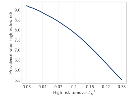
Figure 8: Equilibrium prevalence ratios between high and low risk groups under different rates of turnover.

Turnover rate (log scale) is a function of the duration of time spent in the high risk group $\delta_{H}$, where shorter time spent in the high risk group yields faster turnover. No turnover is indicated by $\delta_{H}^{-1}=0.03$, due to population exit rate $\mu=0.03$.

3.2 Experiment 2: Inferred risk heterogeneity with versus without turnover

After model fitting, our two STI transmission models (one with turnover and one without turnover) reproduced the target equilibrium STI prevalence values of 20%, 8.75%, 3%, and 5% in the high, medium, low risk groups, and total population, respectively (Table 3.2; Figure 3.2). When fitting the model with turnover to these group-specific prevalence targets, the fitted numbers of partners per year $C_{i}$ (the only non-fixed parameter) had to compensate for the reduction in STI prevalence ratio between high and low risk groups (Figure 8). As a result, the ratio of fitted partner numbers between high and low risk groups ($C_{H}~{}/~{}C_{L}$) had to be higher in the model with turnover compared to the model without turnover: $23.9$ vs $15.2$ (Table 3.2). That is, the inferred level of risk heterogeneity was higher in the model with turnover than in the model without turnover.

Table 3: Equilibrium partnership formation rates and prevalence among the high and low risk groups predicted by the models with and without turnover, before and after model fitting.

Number of Partners Prevalence Context High Low High/Low High Low High/Low Turnover & 1.0 25.0 21.6% 3.2% 6.7 No Turnover 25.0 1.0 25.0 21.9% 2.4% 9.2 Turnover [fit] 24.3 1.0 23.9 20.0% 3.0% 6.7 No Turnover [fit] 23.5 1.5 15.2 20.0% 3.0% 6.7

3.3 Experiment 3: Influence of turnover on the tPAF of the high risk group

Finally, we compared the tPAF of the high risk group projected by the fitted model with turnover and the fitted model without turnover (Figure 9). The tPAF projected by both models increased over longer and longer time horizons, indicating that unmet prevention and treatment needs of the high risk group were central to epidemic persistence in both fitted models. The model with turnover projected a larger tPAF at all time-horizons compared with the tPAF projected by the model without turnover. The larger tPAF projected by the model with turnover stemmed from more risk heterogeneity (Table 3.2) which led to more onward transmission from the unmet prevention and treatment needs of the high risk group.

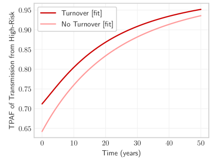
Figure 9: Transmission population attributable fraction (tPAF) of the high risk group in models with and without turnover, after fitting the number of partners per year to group-specific prevalence.

4 Discussion

Using a mechanistic modelling analysis, we found that turnover could be important when projecting the tPAF of high risk groups to the overall epidemic. Mechanistic insights include disentangling three key phenomena by which turnover alters equilibrium STI prevalence within risk groups, and thereby the level of inferred risk heterogeneity between groups via model fitting. Methodological contributions include a framework for modelling turnover which uses a flexible combination of data-driven constraints. Taken together, our explanatory insights and framework have mechanistic, public health, and methodological relevance for the parameterization and use of epidemic models to project intervention priorities for high risk groups.

Influence of turnover on prevalence

Building on prior work by Stigum et al. [40], Zhang et al. [45], Henry and Koopman [18] which similarly found an inverted U-shaped relationship between turnover and overall equilibrium STI prevalence, we identified three key phenomena that generated this relationship. These turnover-driven phenomena were: 1) a net flow of infectious individuals from higher risk groups to lower risk groups; 2) reduced herd immunity in the higher risk groups due to net gain of susceptible individuals; and 3) reduced incidence overall due to fewer partner numbers among infectious individuals. The above three phenomena contributed to the pattern of declining prevalence ratio between the highest and lowest risk groups for increasing rates of turnover. A decline in prevalence ratio due to turnover implies a reduction in risk heterogeneity. Since risk heterogeneity is associated with epidemic emergence and persistence [31] – i.e. the basic reproductive number – our findings are thus consistent with Henry and Koopman [18], who demonstrated that turnover reduces the basic reproductive number by reducing heterogeneity. Indeed, epidemiological and transmission modelling studies have shown that prevalence ratios are an important marker of risk heterogeneity, and in turn the impact of interventions focused on high risk groups [3, 32].

Implications for interventions

Our comparison of fitted models with and without turnover showed that if turnover exists in a given setting but is ignored in a model, the inferred heterogeneity in risk would be lower than in reality, while reproducing the same STI prevalence in each risk group. As a result, the projected tPAF of high risk groups could be systematically underestimated by models that ignore turnover. Although we examined a single parameter to capture risk (number of partners per year), the findings would hold for any combination of factors that alter the risk per susceptible individual (force of infection), including biological transmission probabilities and rates of partner change [2]. The public health implications of models ignoring turnover, and thereby underestimating risk heterogeneity and the tPAF of high risk groups, is that resources could potentially be misguided away from high risk groups. For example, epidemic models which fail to include or accurately capture turnover may underestimate the importance of addressing the unmet needs of key populations at disproportionate risk of HIV and other STIs, such as gay men and other men who have sex with men, transgender women, people who use drugs, and sex workers. In many HIV epidemic models of regions with high HIV prevalence, such as in Southern Africa, key populations have historically been subsumed into the overall modelled population; which meant, by design, less risk heterogeneity [12, 9, 34]. Our findings suggest that even when key populations are included, it is important to further capture within-person changes in risks over time (such as duration in sex work). Underestimating risk heterogeneity could also underestimate the resources required to achieve local epidemic control, as suggested by Henry and Koopman [18], Hontelez et al. [19]. Important next steps surrounding the potential bias in tPAF projections attributable to inclusion/exclusion of turnover include quantifying the magnitude of bias, and characterizing the epidemiologic conditions under which the bias would be meaningfully large in the context of public health programmes.

Turnover framework

We developed a unified framework to parameterize risk group turnover using available epidemiologic data and/or assumptions. There are four potential benefits of using the framework to model turnover. First, the framework defines how specific epidemiologic data and assumptions could be used as constraints to help define rates of turnover. Second, the framework allows flexibility in which constraints can be chosen and combined, so that the constraints best reflect locally available data and/or plausible assumptions. In fact, the framework can adequately reproduce several prior implementations of turnover in various epidemic models [40, 11, 18]. Third, this flexible approach also allows the framework to scale to any number of risk groups. Finally, the framework avoids the need for a burn-in period to establish a demographic steady-state before introducing infection, which was required in some previous models [7].

As noted above, one benefit of the unified framework for modelling turnover is clarifying data priorities for parameterizing turnover. Absolute or relative population size estimates across risk groups may be obtained from population-based sexual behaviour surveys [41], and from mapping and enumeration of marginalized persons such as sex workers [1]. The proportion of individuals who enter into each risk group may be available through sexual behaviour surveys: for example, among individuals who became sexually active for the first time in the past year, the proportion who also engaged in multiple partnerships within the past year. The average duration of time spent within each risk group, such as the duration in sex work, may be drawn from cross-sectional survey questions such as “for how many years have you been a sex worker?” albeit with the recognition that such data are censured [43]. Longitudinal, or cohort studies that track self-reported sexual behaviour over time can also provide estimates of duration of time spent within a given risk strata [14], or provide direct estimates of transition rates between risk strata.

Limitations

Our framework for modelling turnover was developed specifically to answer mechanistic questions about the tPAF; as such, there are two key limitations of the framework in its current form. First, the framework did not stratify the population by sex or age. In the context of real-world STI epidemics, the relative size of risk groups may differ by both sex and age, such as the often smaller number of females and/or males who sell sex, versus the larger number of males who pay for sex (clients of female or male sex workers). Second, the framework does not account for infection-attributable mortality, such as HIV-attributable mortality. However, modelling studies have shown that HIV-attributable mortality can reduce the relative size of higher risk groups who bear a disproportionate burden of HIV, which in turn can cause an HIV epidemic to decline [6]. As such, many models of HIV transmission that include very small ($<3\%$ of the population) high risk groups, such as female sex workers, often do not constrain the relative size of the sub-group populations to be stable over time [36]. By ignoring infection-attributable mortality, the proposed framework would similarly allow risk groups to change relative size in response to disproportionate infection-attributable mortality. Future modifications of the proposed framework include methods to optionally re-balance infection-attributable mortality, and relevant age-sex stratifications so that the framework can be applied more broadly to pathogen-specific epidemics.

Our analyses of turnover and tPAF also have several limitations. First, we did not capture the possibility that some individuals may become re-susceptible to infection after treatment – an important feature of many STIs such as syphilis and gonorrhoea [13]. As shown by Fenton et al. [13] and Pourbohloul et al. [37], the re-supply of susceptible individuals following STI treatment could fuel an epidemic, and so the influence of turnover on STI prevalence and tPAF may be different. Second, our analyses were restricted to equilibrium STI prevalence. The influence of turnover on prevalence and tPAF may vary within different phases of an epidemic – growth, mature, declining [42]. Finally, our analyses reflected an illustrative STI epidemic in a population with illustrative risk strata. Important next steps in the examination of the extent to which turnover influences the tPAF include pathogen- and population-specific modelling – such as the comparisons of model structures by Hontelez et al. [19], Johnson and Geffen [21] – and at different epidemic phases.

Conclusion

In conclusion, turnover may influence prevalence of infection, and thus influence inference on risk heterogeneity when fitting risk-stratified epidemic models. If models do not capture turnover, the projected contribution of high risk groups, and thus, the potential impact of prioritizing interventions to meet their needs, could be underestimated. To aid the next generation of epidemic models used to estimate the tPAF of high risk groups – including key populations – data collection efforts to parameterize risk group turnover should be prioritized.

Acknowledgements

We would like to thank Kristy Yiu (Unity Health Toronto) for logistical support, the Siyaphambili research team for helpful discussions, and Carly Comins (Johns Hopkins University) for facilitating the modelling discussions with the wider study team. SM is supported by an Ontario HIV Treatment Network and Canadian Institutes of Health Research New Investigator Award.

Contributions

JK and SM conceptualized the study and drafted the manuscript; JK designed the experiments with input from LW, HM, and SM. JK developed the unified framework and conducted the modelling, experiments, and analyses; conducted the literature review, and drafted the first version of the manuscript. LW, HM, SB, and SS led substantial structural revisions to the manuscript, including assessment of epidemiological constraints and assumptions; and provided critical discussion surrounding implications of findings. All authors contributed to interpretation of the results and manuscript revision.

Funding

The study was supported by the National Institutes of Health, Grant number: NR016650; the Center for AIDS Research, Johns Hopkins University through the National Institutes of Health, Grant number: P30AI094189.

Conflicts of Interest

Declarations of interest: none.

References

Appendix A Turnover Framework

We introduce a system of parameters and constraints to describe risk group turnover in deterministic epidemic models with heterogeneity in risk. We then describe how the system can be used in practical terms, based on different assumptions and data available for parameterizing turnover in risk. We conclude by framing previous approaches to this task using the proposed system.

A.1 Notation

Consider a population divided into $G$ risk groups. We denote the number of individuals in risk group $i\in[1,\dots,G]$ as $x_{i}$ and the set of all risk groups as $\bm{x}=\{x_{1},\dots,x_{G}\}$. The total population size is $N=\sum_{i}{x_{i}}$, and the relative population size of each group is denoted as $\hat{x}_{i}=x_{i}/N$. Individuals enter the population at a rate $\nu$ per year, and exit at a rate $\mu$ per year. We model the distribution of risk groups among individuals entering into the population as $\bm{\hat{e}}$, which may be different from individuals already in the population $\bm{\hat{x}}$. Thus, the total number of individuals entering into population $\bm{x}$ per year is given by $\nu N$, and the number of individuals entering into group $i$ specifically is given by $\hat{e}_{i}\nu N$.

Turnover transitions may then occur between any two groups, in either direction. Therefore we denote the turnover rates as a $G\times G$ matrix $\phi$. The element $\phi_{ij}$ corresponds to the proportion of individuals in group $i$ who move from group $i$ to group $j$ each year. An example matrix is given in Eq. (A.1), where we write the diagonal elements as $*$ since they represent transitions from a group to itself.

$$\phi=\left[\begin{array}[]{cccc}*&x_{1}\rightarrow x_{2}&\cdots&x_{1}\rightarrow x_{G}\\[4.5pt] x_{2}\rightarrow x_{1}&*&\cdots&x_{2}\rightarrow x_{G}\\[4.5pt] \vdots&\vdots&\ddots&\vdots\\[4.5pt] x_{G}\rightarrow x_{1}&x_{G}\rightarrow x_{2}&\cdots&*\end{array}\right]$$ (A.1)

Risk groups, transitions, and the associated rates are also shown for $G=3$ in Figure A.1.

Figure A.1: System of $G=3$ risk groups and turnover between them.

$x_{i}$: number of individuals in risk group $i$; $e_{i}$: number of individuals available to enter risk group $i$; $\nu$: rate of population entry; $\mu$: rate of population exit; $\phi_{ij}$: rate of turnover from group $i$ to group $j$.

A.2 Parameterization

Next, we present methods to illustrate how epidemiologic data can be used to parametrize turnover in epidemic models. We construct a system like the one above which reflects the risk group dynamics observed in a specific context. We assume that the relative sizes of the risk groups in the model ($\bm{\hat{x}}$) are already known, and should remain constant over time. Thus, what remains is to estimate the values of the parameters: $\nu$, $\mu$, $\bm{\hat{e}}$, and $\phi$, using commonly available sources of data.

A.2.1 Total Population Size

The total population size $N(t)$ is a function of the rates of population entry $\nu(t)$ and exit $\mu(t)$, given an initial size $N_{0}$. We allow the proportion entering the system to vary by risk group via $\bm{\hat{e}}$, while the exit rate has the same value for each group. We assume that there is no disease-attributable death. Because the values of $\nu$ and $\mu$ are the same for each risk group, they can be estimated independent of $\bm{\hat{x}}$, $\bm{\hat{e}}$, and $\phi$.

The difference between entry and exit rates defines the rate of population growth:

$$\mathcal{G}(t)=\nu(t)-\mu(t)$$ (A.2)

The total population may then be defined using an initial population size $N_{0}$ as:

$$N(t)=N_{0}\exp{\left(\int_{0}^{\,t}{\log\big{(}1+\mathcal{G}(\tau)\big{)}d\tau}\right)}$$ (A.3)

which, for constant growth, simplifies to the familiar expression [29]:

$$N(t)=N_{0}{(1+\mathcal{G})}^{t}$$ (A.4)

Census data, such as [10], can be used to source the total population size in a given geographic setting over time $N(t)$, thus allowing Eqs. (A.3) and (A.4) to be used to estimate $\mathcal{G}(t)$.

If the population size is assumed to be constant, then $\mathcal{G}(t)=0$ and $\nu(t)=\mu(t)$. If population growth occurs at a stable rate, then $\mathcal{G}$ is fixed at a constant value which can be estimated via Eq. (A.4) using any two values of $N(t)$, separated by a time interval $\tau$:

$$\mathcal{G}_{\tau}={\frac{N(t+\tau)}{N(t)}}^{\frac{1}{\tau}}-1$$ (A.5)

If the rate of population growth $\mathcal{G}$ varies over time, then Eq. (A.5) can be reused for consecutive time intervals, and the complete function $\mathcal{G}(t)$ approximated piecewise by constant values. The piecewise approximation can be more feasible than exact solutions using Eq. (A.3), and can reproduce $N(t)$ accurately for small enough intervals $\tau$, such as one year.

Now, given a value of $\mathcal{G}(t)$, either $\nu(t)$ must be chosen and $\mu(t)$ calculated using Eq. (A.2), or $\mu(t)$ must be chosen, and $\nu(t)$ calculated. Most modelled systems assume a constant duration of time that individuals spend in the model $\delta(t)$ [2] which is related to the rate of exit $\mu$ by:

$$\delta(t)=\mu^{-1}(t)$$ (A.6)

In the context of sexually transmitted infections, the duration of time usually reflects the average sexual life-course of individuals from age 15 to 50 years, such that $\delta=35$ years. The duration $\delta$ may also vary with time to reflect changes in life expectancy. The exit rate $\mu(t)$ can then be defined as $\delta^{-t}(t)$ following Eq. (A.6), and the entry rate $\nu(t)$ defined as $\mathcal{G}(t)-\mu(t)$ following Eq. (A.2).

A.2.2 Turnover

Next, we present methods for resolving the distribution of individuals entering the risk model $\bm{\hat{e}}(t)$ and the rates of turnover $\phi(t)$, assuming that entry and exit rates $\nu(t)$ and $\mu(t)$ are known. Similar to above, we first formulate the problem as a system of equations. Then, we explore the data and assumptions required to solve for the values of parameters in the system. The $(t)$ notation is omitted throughout this section for clarity, though time-varying parameters can be estimated by repeating the necessary calculations for each $t$.

The number of risk groups $G$ dictates the number of unknown elements in $\bm{\hat{e}}$ and $\phi$: $G$ and $G(G-1)$, respectively. We collect these unknowns in the vector $\bm{\theta}=\left[\bm{\hat{e}},\bm{y}\right]$, where $\bm{y}=\mathrm{vec}_{i\neq j}(\phi)$. For example, for $G=3$, the vector $\bm{\theta}$ is defined as:

$$\bm{\theta}=\left[\begin{array}[]{ccccccccc}\hat{e}_{1}&\hat{e}_{2}&\hat{e}_{3}&\phi_{12}&\phi_{13}&\phi_{21}&\phi_{23}&\phi_{31}&\phi_{32}\end{array}\right]$$ (A.7)

We then define a linear system of equations which uniquely determine the elements of $\bm{\theta}$:

$$\bm{b}=A\thinspace\bm{\theta}$$ (A.8)

where $A$ is a $M\times G^{2}$ matrix and $\bm{b}$ is a $M$-length vector. Specifically, each row in $A$ and $\bm{b}$ defines a constraint: an assumed mathematical relationship involving one or more elements of $\bm{\hat{e}}$ and $\phi$. For example, a simple constraint could be to assume the value $\hat{e}_{2}=0.20$. Each of the following four sections introduces a type of constraint, including: assuming a constant group size, specifying elements of $\bm{\theta}$ directly, assuming an average duration in a group, and specifying a relationship between two individual rates of turnover. Constraints may be selected and combined together based on availability of data and plausibility of assumptions. However, a total of $M=G^{2}$ constraints must be defined in order to obtain a “unique solution”: exactly one value of $\bm{\theta}$ which satisfies all constraints. The values of $\bm{\hat{e}}$ and $\phi$ can then be calculated algebraically by solving Eq. (A.8) with $\bm{\theta}=A^{-1}\bm{b}$, for which many algorithms exist [25].

1. Constant group size

One epidemiologic feature that epidemic models consider is whether or not the relative sizes of risk groups are constant over time [18, 7]. Assuming constant group size implies a stable level of heterogeneity over time. To enforce this assumption, we define the “conservation of mass” equation for group $i$, wherein the rate of change of the group is defined as the sum of flows in / out of the group:

$$\frac{d}{dt}x_{i}=\nu N\hat{e}_{i}+\sum_{j}{\phi_{ji}\thinspace x_{j}}-\mu\thinspace x_{i}-\sum_{j}{\phi_{ij}\thinspace x_{i}}$$ (A.9)

Eq. (A.9) is written in terms of absolute population sizes $\bm{x}$, but can be written as proportions $\bm{\hat{x}}$ by dividing all terms by $N$. If we assume that the proportion of each group $\hat{x}_{i}$ is constant over time, then the desired rate of change for risk group $i$ will be equal to the rate of population growth of the risk group, $\mathcal{G}x_{i}$. Substituting $\frac{d}{dt}x_{i}=\mathcal{G}x_{i}$ into Eq. (A.9), and simplifying yields:

$$\nu\thinspace x_{i}=\nu\thinspace N\hat{e}_{i}+\sum_{j}{\phi_{ji}\thinspace x_{j}}-\sum_{j}{\phi_{ij}\thinspace x_{i}}$$ (A.10)

Factoring the left and right hand sides in terms of $\bm{\hat{e}}$ and $\phi$, we obtain $G$ unique constraints. For $G=3$, this yields the following 3 rows as the basis of $\bm{b}$ and $A$:

$$\bm{b}=\left[\begin{array}[]{c}\nu x_{1}\\ \nu x_{2}\\ \nu x_{3}\end{array}\right];\qquad A=\left[\begin{array}[]{ccccccccc}\nu&\cdot&\cdot&-x_{1}&-x_{1}&x_{2}&\cdot&x_{3}&\cdot\\ \cdot&\nu&\cdot&x_{1}&\cdot&-x_{2}&-x_{2}&\cdot&x_{3}\\ \cdot&\cdot&\nu&\cdot&x_{1}&\cdot&x_{2}&-x_{3}&-x_{3}\end{array}\right]$$ (A.11)

These $G$ constraints ensure risk groups do not change size over time. However, a unique solution requires an additional $G(G-1)$ constraints. For $G=3$, this corresponds to 6 additional constraints.

2. Specified elements

The simplest type of additional constraint is to directly specify the values of individual elements in $\bm{\hat{e}}$ or $\phi$. Such constraints may be appended to $\bm{b}$ and $A$ as an additional row $k$ using indicator notation. That is, with $b_{k}$ as the specified value $v$, and $A_{k}$ as the indicator vector, with $1$ in the same position as the desired element in $\bm{\theta}$:

$$b_{k}=v;\qquad A_{k}=[0,\dots,1,\dots,0]$$ (A.12)

For example, for $G=3$, if it is known that 20% of individuals enter directly into risk group $2$ upon entry into the model ($\hat{e}_{2}=0.20$), then $\bm{b}$ and $A$ can be augmented with:

$$b_{k}=\left[\begin{array}[]{c}0.20\end{array}\right];\qquad A_{k}=\left[\begin{array}[]{ccccccccc}\cdot&1&\cdot&\cdot&\cdot&\cdot&\cdot&\cdot&\cdot\end{array}\right]$$ (A.13)

since $\hat{e}_{2}$ is the second element in $\bm{\theta}$. If the data suggest zero turnover from group $i$ to group $j$, then Eq. (A.13) can also be used to set $\phi_{ij}=0$.

The elements of $\bm{\hat{e}}$ must sum to one. Therefore, specifying all elements in $\bm{\hat{e}}$ will only provide $G-1$ constraints, as the last element will be either redundant or violate the sum-to-one rule. As shown in Appendix B.3, the sum-to-one rule is actually implicit in Eq. (A.11), so it is not necessary to supply a constraint like $1=\sum_{i}\hat{e}_{i}$.

3. Group duration

Type 1 constraints assume that the relative population size of each group remains constant. Another epidemiologic feature that epidemic models considered is whether or not the duration of time spent within a given risk group remains constant. For example, in STI transmission models that include formal sex work, it can be assumed that the duration in formal sex work work remains stable over time, such as in [33, 7]. The duration $\delta_{i}$ is defined as the inverse of all rates of exit from the group:

$$\delta_{i}={\bigg{(}\mu+\sum_{j}{\phi_{ij}}\bigg{)}}^{-1}$$ (A.14)

Estimates of the duration in a given group can be sourced from cross-sectional survey data where participants are asked about how long they have engaged in a particular practice – such as sex in exchange for money [43]. Data on duration may also be sourced from longitudinal data, where repeated measures of self-reported sexual behaviour, or proxy measures of sexual risk data, are collected [41, 20]. Data on duration in each risk group can then be used to define $\phi$ by rearranging Eq. (A.14) to yield: ${\delta_{i}}^{-1}-\mu=\sum_{j}{\phi_{ij}}$. For example, if for $G=3$, the average duration in group $1$ is known to be $\delta_{1}=5$ years, then $\bm{b}$ and $A$ can be augmented with another row $k$:

$$b_{k}=\left[\begin{array}[]{c}{5}^{-1}-\mu\end{array}\right];\qquad A_{k}=\left[\begin{array}[]{ccccccccc}\cdot&\cdot&\cdot&1&1&\cdot&\cdot&\cdot&\cdot\end{array}\right]$$ (A.15)

Similar to specifying all elements of $\bm{\hat{e}}$, specifying $\delta_{i}$ may result in conflicts or redundancies with other constraints. A conflict means it will not be possible to resolve values of $\phi$ which simultaneously satisfy all constraints, while a redundancy means that adding one constraint does not help resolve a unique set of values $\bm{\theta}$. For example, for $G=3$, if Type 2 constraints are used to specify $\phi_{12}=0.1$ and $\phi_{13}=0.1$, and $\mu=0.05$, then by Eq. (A.14), we must have $\delta_{1}=4$. Specifying any other value for $\delta_{1}$ will result in a conflict, while specifying $\delta_{1}=4$ is redundant, since it is already implied. There are innumerable situations in which this may occur, so we do not attempt to describe them all. Section A.2.2 describes how to identify conflicts and redundancies when they are not obvious.

4. Turnover rate ratios

In many cases, it may be difficult to obtain estimates of a given turnover rate $\phi_{ij}$ for use in Type 2 constraints. However, it may be possible to estimate relative relationships between rates of turnover, such as:

$$r\,\phi_{ij}=\phi_{i^{\prime}j^{\prime}}$$ (A.16)

where $r$ is a ratio relating the values of $\phi_{ij}$ and $\phi_{i^{\prime}j^{\prime}}$. For example, for $G=3$, let $T_{1}$ be the total number of individuals entering group $1$ due to turnover. If we know that 70% of $T_{1}$ originates from group $2$, while 30% of $T_{1}$ originates from group $3$, then $0.7\,T_{1}=\phi_{23}\,x_{2}$ and $0.3\,T_{1}=\phi_{13}\,x_{1}$, and thus: $\phi_{23}\left(\frac{0.3\,x_{2}}{0.7\,x_{1}}\right)=\phi_{13}$. This constraint can then be appended as another row $k$ in $\bm{b}$ and $A$ like:

$$b_{k}=\left[\begin{array}[]{c}0\end{array}\right];\qquad A_{k}=\left[\begin{array}[]{ccccccccc}\cdot&\cdot&\cdot&\cdot&\left(\frac{0.3\,x_{2}}{0.7\,x_{1}}\right)&\cdot&1&\cdot&\cdot\end{array}\right]$$ (A.17)

The example in Eq. (A.17) is based on what proportions of individuals entering a risk group $j$ came from which former risk group $i$, but similar constraints may be defined based on what proportions of individuals exiting a risk group $i$ enter into which new risk group $j$. It can also be assumed that the absolute number of individuals moving between two risk groups is equal, in which case the relationship is: $\phi_{ij}\left(\frac{x_{i}}{x_{j}}\right)=\phi_{ji}$. All constraints of this type will have $b_{k}=0$.

Solving the System

Table A.2.2 summarizes the four types of constraints described above. Given a set of sufficient constraints on $\bm{\theta}$ to ensure exactly one solution, the system of equations Eq. (A.8) can be solved using $\bm{\theta}=A^{-1}\bm{b}$. The resulting values of $\bm{\hat{e}}$ and $\phi$ can then be used in the epidemic model.

However, we may find that we have an insufficient number of constraints, implying that there are multiple values of the vector $\bm{\theta}$ which satisfy the constraints. An insufficient number of constraints may be identified by a “rank deficiency” warning in numerical solvers of Eq. (A.8) [25]. Even if $A$ has $G^{2}$ rows, the system may have an insufficient number of constraints because some constraints are redundant. In this situation, we can pose the problem as a minimization problem, namely:

$$\bm{\theta}^{*}={\arg\min}\thinspace f(\bm{\theta}),\quad\textrm{subject to:}\enspace\bm{b}=A\thinspace\bm{\theta};\enspace\bm{\theta}\geq 0$$ (A.18)

where $f$ is a function which penalizes certain values of $\bm{\theta}$. For example, $f={\left|\left|\,\cdot\,\right|\right|}_{2}$ penalizes large values in $\bm{\theta}$, so that the smallest values of $\bm{\hat{e}}$ and $\phi$ which satisfy the constraints will be resolved.

Similarly, we may find that no solution exists for the given constraints, since two or more constraints are in conflict. Conflicting constraints may be identified by a non-zero error in the solution to Eq. (A.8) [25]. In this case, the conflict should be resolved by changing or removing one of the conflicting constraints.

Table A.1: Summary of constraint types for defining risk group turnover

$\nu$: rate of population entry; $\phi_{ij}$: rate of turnover from group $i$ to group $j$; $\hat{x}_{i}$: proportion of individuals in risk group $i$; $\hat{e}_{i}$: proportion of individuals entering into risk group $i$; $\delta_{i}$: average duration spent in risk group $i$.

A.3 Previous Approaches

Few epidemic models of sexually transmitted infections with heterogeneity in risk have simulated turnover among risk groups, and those models which have simulated turnover have done so in various ways. In this section, we review three prior implementations of turnover and their assumptions. We then highlight how the approach proposed in Section A.2 could be used to achieve the same objectives.

Stigum et al. [40] simulated turnover among $G=2$ risk groups in a population with no exogenous entry or exit ($\nu=\mu=0$ and hence $\bm{\hat{e}}$ is not applicable). Turnover between the groups was balanced in order to maintain constant risk group sizes (Type 1 constraint), while the rate of turnover from high to low was specified as $\kappa$ (Type 2 constraint). Thus, the turnover system used by Stigum et al. [40] can be written in the proposed framework as:

$$\left[\begin{array}[]{c}0\\ \kappa\end{array}\right]=\left[\begin{array}[]{cc}\hat{x}_{1}&-\hat{x}_{2}\\ 1&\cdot\end{array}\right]\left[\begin{array}[]{c}\phi_{12}\\ \phi_{21}\end{array}\right],\qquad\hat{e}_{1}=\hat{e}_{2}=0$$ (A.19)

Henry and Koopman [18] also simulated turnover among $G=2$ risk groups, but considered exogenous entry and exit, both at a rate $\mu$. The authors used the notation $f_{i}$ for our $\hat{x}_{i}$, and assumed that the population of individuals entering into the modelled population had the same distribution of risk groups as the modelled population itself: $\hat{e}_{i}=f_{i}$ (Type 2 constraint). The authors further maintained constant risk group sizes (Type 1 constraint) by analytically balancing turnover between the two groups using: $\phi_{12}=\omega\hat{x}_{2};\enspace\phi_{21}=\omega\hat{x}_{1}$, where $\omega$ is a constant. However, it can be shown that this analytical approach is also the solution to the following combination of Type 1 and Type 2 constraints:

$$\left[\begin{array}[]{c}0\\ \omega f_{2}\end{array}\right]=\left[\begin{array}[]{cc}f_{1}&-f_{2}\\ 1&\cdot\end{array}\right]\left[\begin{array}[]{c}\phi_{12}\\ \phi_{21}\end{array}\right],\qquad\hat{e}_{i}=f_{i}$$ (A.20)

Eaton and Hallett [11] simulated turnover among $G=3$ risk groups, considering a distribution of risk among individuals entering into the modelled population $\bm{\hat{e}}$ which was different from $\bm{\hat{x}}$. Turnover was considered from high-to-medium, high-to-low, and medium-to-low risk, all with an equal rate $\psi$; the reverse transition rates were set to zero (six total Type 2 constraints). Given the unidirectional turnover, risk group sizes were maintained using the values of $\hat{e}_{i}$, computed using Type 1 constraints as follows:

$$\left[\begin{array}[]{l}\nu x_{1}+2x_{1}\psi\\ \nu x_{2}-x_{1}\psi+x_{2}\psi\\ \nu x_{3}-x_{1}\psi-x_{2}\psi\end{array}\right]=\left[\begin{array}[]{ccc}\nu&\cdot&\cdot\\ \cdot&\nu&\cdot\\ \cdot&\cdot&\nu\\ \end{array}\right]\left[\begin{array}[]{c}e_{1}\\ e_{2}\\ e_{3}\end{array}\right],\qquad\begin{array}[]{c}\phi_{12}=\phi_{13}=\phi_{23}=\psi\\ \phi_{21}=\phi_{31}=\phi_{32}=0\end{array}$$ (A.21)

In sum, the framework for modelling turnover presented in this section aims to generalize all previous implementations. In so doing, we hope to clarify the requisite assumptions, dependencies on epidemiologic data, and relationships between previous approaches.

Appendix B Supplemental Equations

Table B.1: Notation

Symbol	Definition
$i$	risk group index
$j$	risk group index for “other” group in turnover
$k$	risk group index for “other” group in incidence
$t$	time
$\mathcal{S}_{i}$	number of susceptible individuals in risk group $i$
$\mathcal{I}_{i}$	number of infectious individuals in risk group $i$
$\mathcal{T}_{i}$	number of treated individuals in risk group $i$
$N$	total population size
$\nu$	rate of population entry
$\mu$	rate of population exit
$\phi_{ij}$	rate of turnover from group $i$ to group $j$
$\lambda_{i}$	force of infection among susceptibles in risk group $i$
$\tau$	rate of treatment initiation among infected
$\hat{x}_{i}$	proportion of individuals in risk group $i$
$\hat{e}_{i}$	proportion of individuals entering into risk group $i$
$\delta_{i}$	average duration spent in risk group $i$
$C_{i}$	number of partners per year among individuals in risk group $i$
$\beta$	probability of transmission per partnership
$\rho_{ik}$	probability of partnership formation between risk groups $i$ and $k$

B.1 Model Equations

$$\frac{d}{dt}\mathcal{S}_{i}(t) =+\sum_{j}\phi_{ji}\mathcal{S}_{j}(t) -\sum_{j}\phi_{ij}\mathcal{S}_{i}(t) -\mu\mathcal{S}_{i}(t) +\nu\hat{e}_{i}N(t) -\lambda_{i}(t)\mathcal{S}_{i}(t)$$ (B.1a)

$$\frac{d}{dt}\mathcal{I}_{i}(t) =+\sum_{j}\phi_{ji}\mathcal{I}_{j}(t) -\sum_{j}\phi_{ij}\mathcal{I}_{i}(t) -\mu\mathcal{I}_{i}(t) +\lambda_{i}(t)\mathcal{S}_{i}(t) -\tau\mathcal{I}_{i}(t)$$ (B.1b)

$$\frac{d}{dt}\mathcal{T}_{i}(t) =+\sum_{j}\phi_{ji}\mathcal{T}_{j}(t) -\sum_{j}\phi_{ij}\mathcal{T}_{i}(t) -\mu\mathcal{T}_{i}(t) +\tau\mathcal{I}_{i}(t)$$ (B.1c)

$$\hphantom{=}\underbrace{\smash{\phantom{+\sum_{j}\phi_{ji}\mathcal{S}_{j}(t)}}}_{\textrm{turnover into}} \underbrace{\smash{\phantom{+\sum_{j}\phi_{ij}\mathcal{S}_{i}(t)}}}_{\textrm{turnover from}} \underbrace{\smash{\phantom{+\mu\mathcal{S}_{i}(t)}}}_{\textrm{death}} \underbrace{\smash{\phantom{+\nu\hat{e}_{i}N(t)}}}_{\textrm{birth}} \underbrace{\smash{\phantom{+\lambda_{i}(t)\mathcal{S}_{i}(t)}}}_{\textrm{incidence}} \underbrace{\smash{\phantom{+\tau\mathcal{I}_{i}(t)}}}_{\textrm{treatment}}$$

B.2 Complete Example Turnover System

$$\footnotesize\begin{array}[]{r}\left.\begin{array}[]{c}\\ \textrm{constant group size}\\ \\ \end{array}\right\{\\ \left.\begin{array}[]{c}\\ \textrm{specified $e$}\\ \\ \end{array}\right\{\\ \left.\begin{array}[]{c}\\ \textrm{group duration}\\ \\ \end{array}\right\{\\ \left.\begin{array}[]{c}\\ \textrm{turnover rate ratios}\\ \\ \end{array}\right\{\\ \end{array}\left[\begin{array}[]{c}\nu x_{1}\\ \nu x_{2}\\ \nu x_{3}\\ e^{*}_{1}\\ e^{*}_{2}\\ e^{*}_{3}\\ {\delta_{1}}^{-1}-\mu\\ {\delta_{2}}^{-1}-\mu\\ {\delta_{3}}^{-1}-\mu\\ 0\\ 0\\ 0\end{array}\right]=\left[\begin{array}[]{ccccccccc}\nu&\cdot&\cdot&-x_{1}&-x_{1}&x_{2}&\cdot&x_{3}&\cdot\\ \cdot&\nu&\cdot&x_{1}&\cdot&-x_{2}&-x_{2}&\cdot&x_{3}\\ \cdot&\cdot&\nu&\cdot&x_{1}&\cdot&x_{2}&-x_{3}&-x_{3}\\ 1&\cdot&\cdot&\cdot&\cdot&\cdot&\cdot&\cdot&\cdot\\ \cdot&1&\cdot&\cdot&\cdot&\cdot&\cdot&\cdot&\cdot\\ \cdot&\cdot&1&\cdot&\cdot&\cdot&\cdot&\cdot&\cdot\\ \cdot&\cdot&\cdot&1&1&\cdot&\cdot&\cdot&\cdot\\ \cdot&\cdot&\cdot&\cdot&\cdot&1&1&\cdot&\cdot\\ \cdot&\cdot&\cdot&\cdot&\cdot&\cdot&\cdot&1&1\\ \cdot&\cdot&\cdot&x_{1}&\cdot&-x_{2}&\cdot&\cdot&\cdot\\ \cdot&\cdot&\cdot&\cdot&x_{1}&\cdot&\cdot&-x_{3}&\cdot\\ \cdot&\cdot&\cdot&\cdot&\cdot&\cdot&x_{2}&\cdot&-x_{3}\end{array}\right]\left[\begin{array}[]{c}e_{1}\\ e_{2}\\ e_{3}\\ \phi_{12}\\ \phi_{13}\\ \phi_{21}\\ \phi_{23}\\ \phi_{31}\\ \phi_{32}\\ \end{array}\right]$$ (B.2)

B.3 Redundancy in specifying all elements of $\hat{e}$

Whenever it is assumed that risk groups do not change size, $G$ rows of the form shown in Eq. (A.11) are added to $\bm{b}$ and $A$:

$$\bm{b}=\left[\begin{array}[]{c}\nu x_{1}\\ \nu x_{2}\\ \nu x_{3}\end{array}\right];\qquad A=\left[\begin{array}[]{ccccccccc}\nu&\cdot&\cdot&-x_{1}&-x_{1}&x_{2}&\cdot&x_{3}&\cdot\\ \cdot&\nu&\cdot&x_{1}&\cdot&-x_{2}&-x_{2}&\cdot&x_{3}\\ \cdot&\cdot&\nu&\cdot&x_{1}&\cdot&x_{2}&-x_{3}&-x_{3}\\ \end{array}\right]$$ (A.11)

After multiplying by $\bm{\theta}$, these $G$ rows can be row-reduced by summing to obtain:

$$\left[\nu x_{1}+\nu x_{2}+\nu x_{3}\right] =\left[\nu e_{1}+\nu e_{2}+\nu e_{3}+0\,\phi_{12}+0\,\phi_{13}+0\,\phi_{21}+0\,\phi_{23}+0\,\phi_{31}+0\,\phi_{32}\right]$$ (B.3)

$$\nu\left[x_{1}+x_{2}+x_{3}\right] =\nu\left[e_{1}+e_{2}+e_{3}\right]$$

which therefore implies that $\sum_{i}x_{i}=\sum_{i}e_{i}$, or equivalently $\sum_{i}\hat{x}_{i}=\sum_{i}\hat{e}_{i}=1$. Thus, it is redundant to specify all $G$ elements of $\hat{e}$, as the final element will be dictated by constant group size constraints.

B.4 Factors of Incidence

Substituting the proportional mixing definition of $\rho_{ik}$ into the incidence equation, Eq. (3), we have:

$$\lambda_{i} =C_{i}\sum_{k}\rho_{ik}\beta\thinspace\frac{\mathcal{I}_{k}}{\mathcal{X}_{k}}$$

$$=C_{i}\beta\sum_{k}\frac{C_{k}\mathcal{X}_{k}}{\sum_{\mathrm{k}}C_{\mathrm{k}}\mathcal{X}_{\mathrm{k}}}\frac{\mathcal{I}_{k}}{\mathcal{X}_{k}}$$

$$=C_{i}\beta\underbrace{\frac{\sum_{k}C_{k}\mathcal{I}_{k}}{\sum_{\mathrm{k}}C_{\mathrm{k}}\mathcal{X}_{\mathrm{k}}}}_{f}$$ (B.4)

We can factor the term $f$ as:

$$f =\frac{\sum_{k}C_{k}\mathcal{I}_{k}}{\sum_{\mathrm{k}}C_{\mathrm{k}}\mathcal{X}_{\mathrm{k}}}$$

$$=\frac{\sum_{k}C_{k}\mathcal{I}_{k}}{\sum_{k}\mathcal{I}_{k}}\cdot\frac{\sum_{k}\mathcal{I}_{k}}{\sum_{k}\mathcal{X}_{k}}\cdot\frac{\sum_{k}\mathcal{X}_{k}}{\sum_{k}C_{k}\mathcal{X}_{k}}$$ (B.5)

which we recognize as the following terms:

$$=\hat{C}_{\mathcal{I}}\cdot\hat{\mathcal{I}}\cdot\hat{C}^{-1}$$ (B.6)

Namely,

1. $\hat{C}_{\mathcal{I}}$ is the average number of partners among infectious individuals

2. $\hat{\mathcal{I}}$ is the proportion of the population who are infectious (overall prevalence)

3. $\hat{C}$ is the average number of partners among all individuals (constant)

Therefore, only two non-constant factors control incidence per susceptible: 1) the average number of partners among infectious individuals $\hat{C}_{\mathcal{I}}$, and 2) overall prevalence $\hat{\mathcal{I}}$. The product of these factors $\hat{C}_{\mathcal{I}}\,\hat{\mathcal{I}}$, scaled by $\beta\,C_{i}/\hat{C}$, then gives $\lambda_{i}$. In fact, the incidence in each group individually is proportional to incidence overall, as $C_{i}$ is only factor depending on $i$.

Appendix C Supplemental Results

C.1 Equilibrium health states and rates of transition

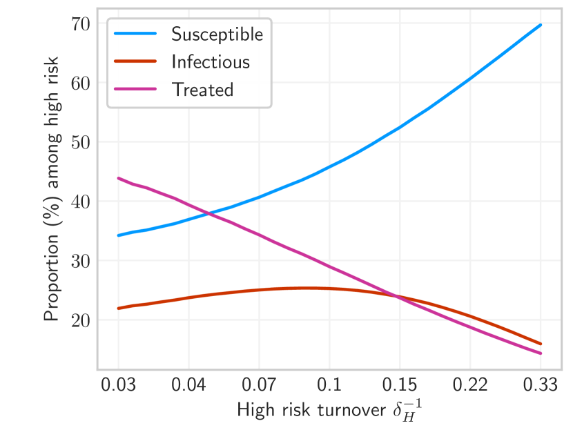
(a) High risk

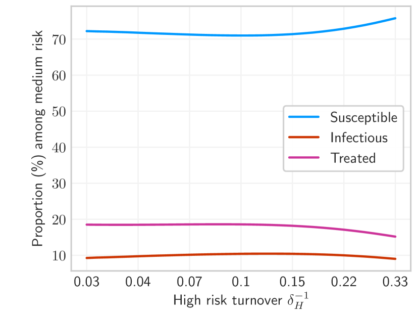
(b) Medium risk

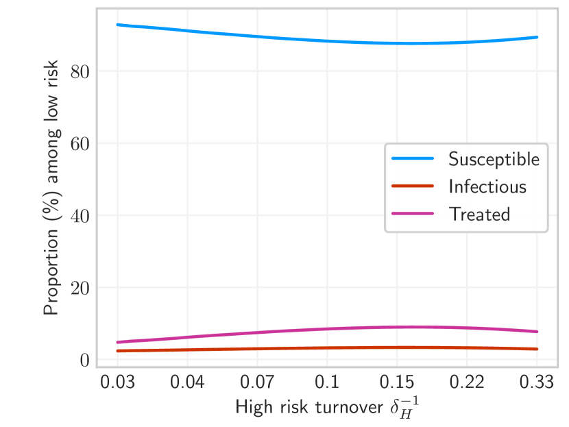
(c) Low risk

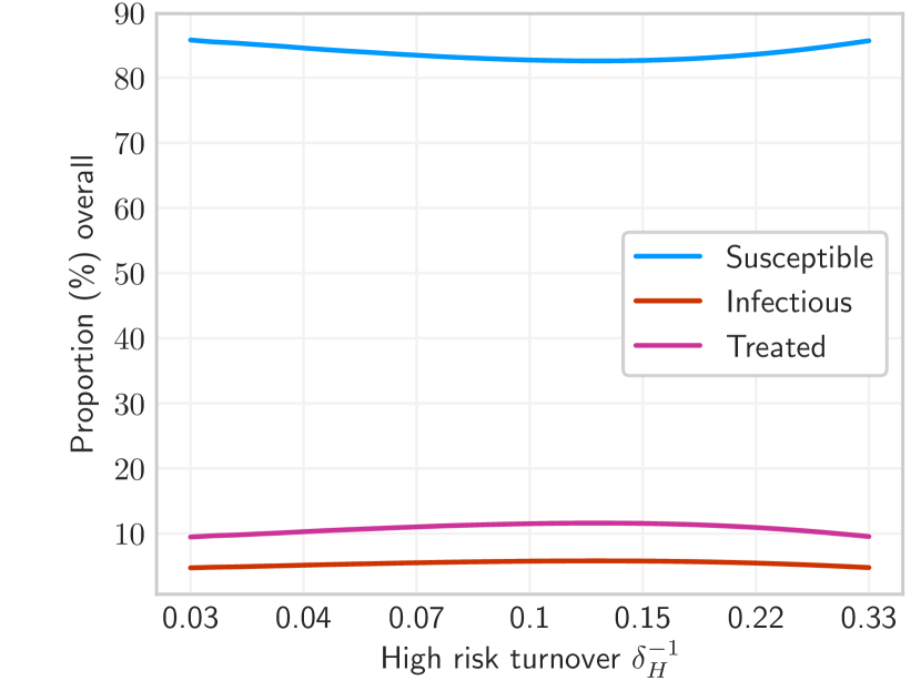
(d) Overall

Figure C.1: Equilibrium health state proportions under different rates of turnover.

Turnover rate (log scale) is a function of the duration of time spent in the high risk group $\delta_{H}$, where shorter time spent in the high risk group yields faster turnover. No turnover is indicated by $\delta_{H}^{-1}=0.03$, due to population exit rate $\mu=0.03$.

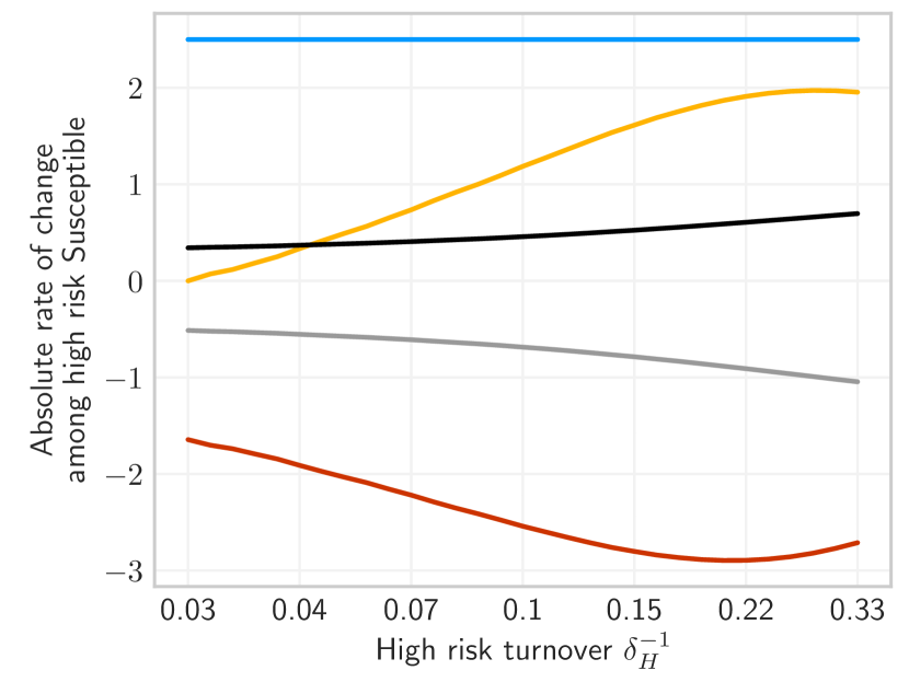
(a) High risk susceptible

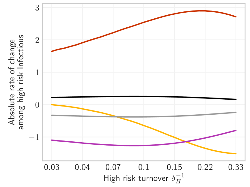
(b) High risk infectious

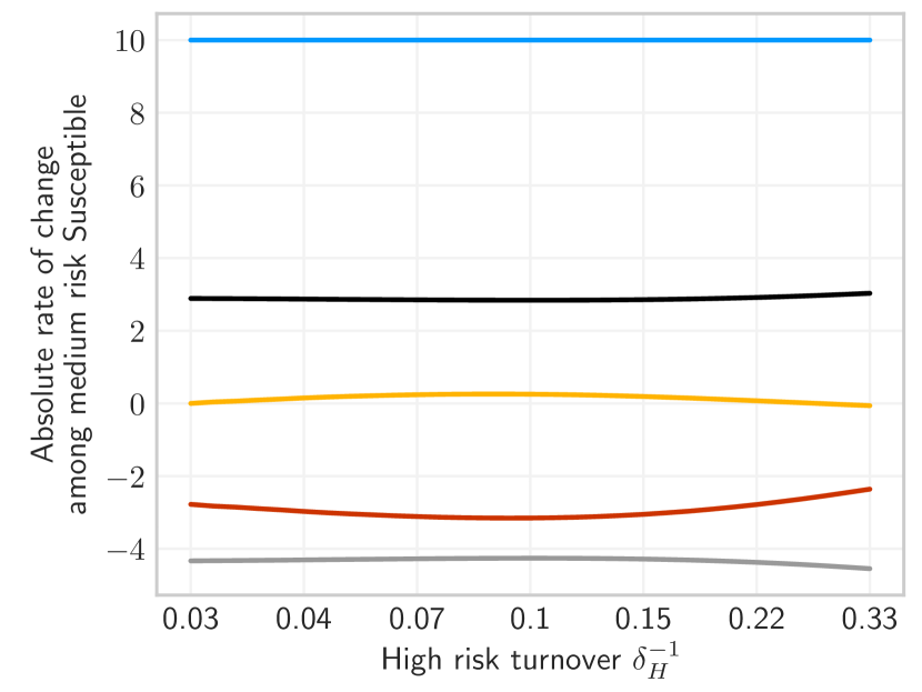
(d) Medium risk susceptible

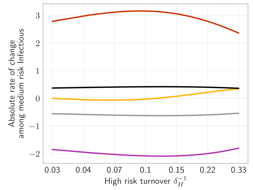
(e) Medium risk infectious

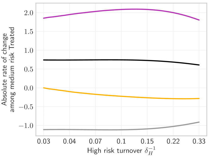
(f) Medium risk treated

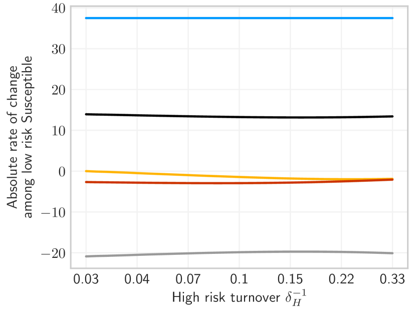
(g) Low risk susceptible

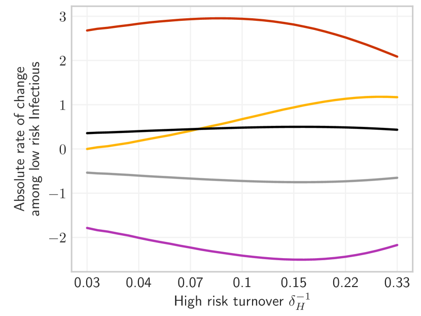
(h) Low risk infectious

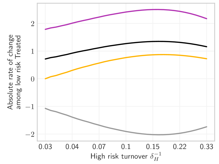
(i) Low risk treated

Figure C.2: Absolute rates of change at equilibrium (number of individuals gained/lost per year) among individuals in each health state and risk group, broken down by type of change: gain via births, loss/gain via incident infections, loss/gain via treatment, loss/gain via turnover, loss via death, and net change. Based on Eq. (B.1).

Turnover rate (log scale) is a function of the duration of time spent in the high risk group $\delta_{H}$, where shorter time spent in the high risk group yields faster turnover. No turnover is indicated by $\delta_{H}^{-1}=0.03$, due to population exit rate $\mu=0.03$. Rates of change do not sum to zero due to population growth.

Figure C.3: Proportion of new infectious individuals in each risk group which are from turnover of infectious individuals, as opposed to incident infection of susceptible individuals in the risk group.

C.2 Equilibrium Prevalence Ratios

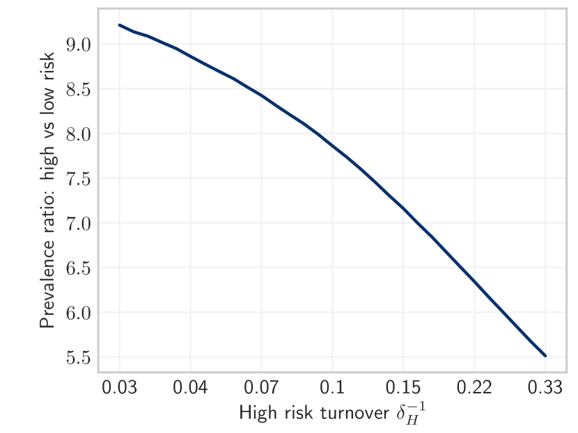
(a) High vs Low risk

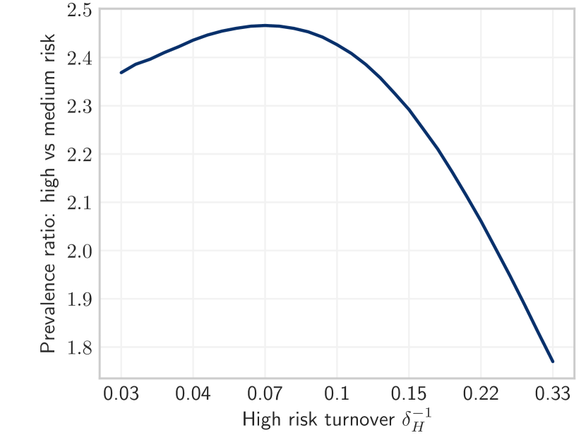
(b) High vs Medium Risk

Figure C.4: Equilibrium prevalence ratios between risk groups under different rates of turnover.

Turnover rate (log scale) is a function of the duration of time spent in the high risk group $\delta_{H}$, where shorter time spent in the high risk group yields faster turnover. No turnover is indicated by $\delta_{H}^{-1}=0.03$, due to population exit rate $\mu=0.03$.

C.3 Equilibrium Incidence

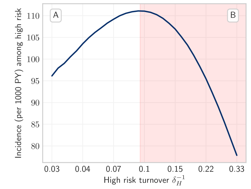
(a) High risk

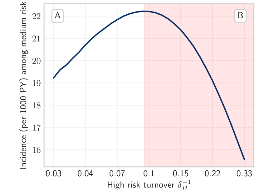
(b) Medium risk

Figure C.5: Equilibrium incidence among high, medium, and low risk groups under different rates of turnover.

Turnover rate (log scale) is a function of the duration of time spent in the high risk group $\delta_{H}$, where shorter time spent in the high risk group yields faster turnover. No turnover is indicated by $\delta_{H}^{-1}=0.03$, due to population exit rate $\mu=0.03$. Incidence in each risk group is proportional to overall incidence with $C_{i}$ as a scale factor.

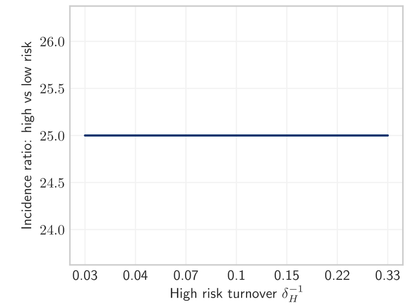
(a) High vs low risk

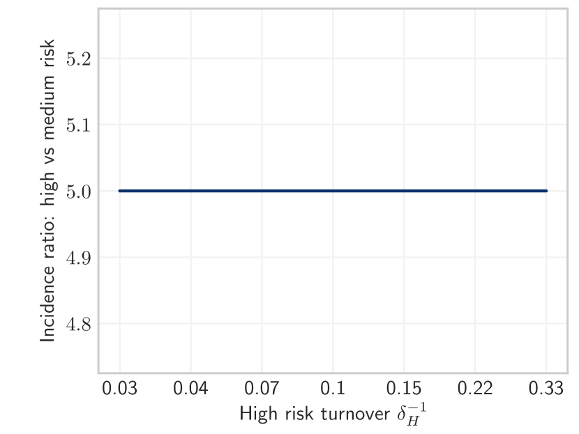
(b) High vs medium risk

(c) Medium vs low risk

Figure C.6: Equilibrium incidence ratios between risk groups under different rates of turnover. Incidence ratios do not depend on turnover.

Turnover rate (log scale) is a function of the duration of time spent in the high risk group $\delta_{H}$, where shorter time spent in the high risk group yields faster turnover. No turnover is indicated by $\delta_{H}^{-1}=0.03$, due to population exit rate $\mu=0.03$.

C.4 Equilibrium prevalence and number of partners before and after model fitting

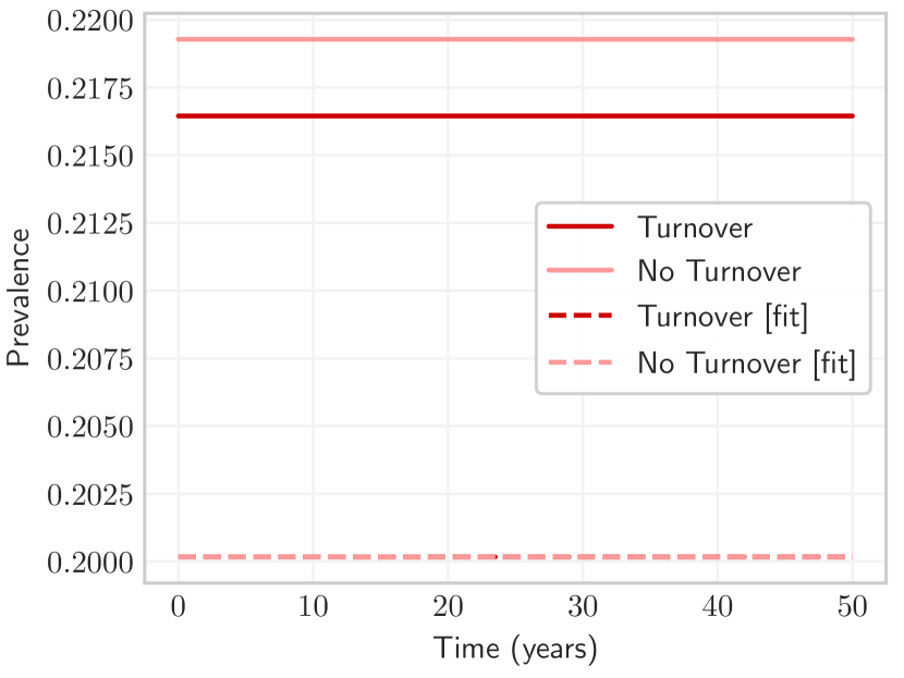
(a) High risk

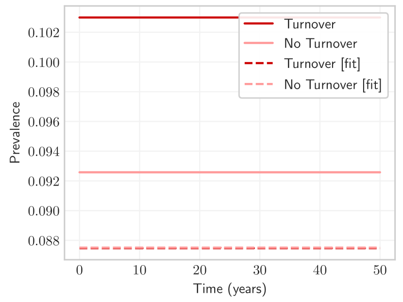
(b) Medium risk

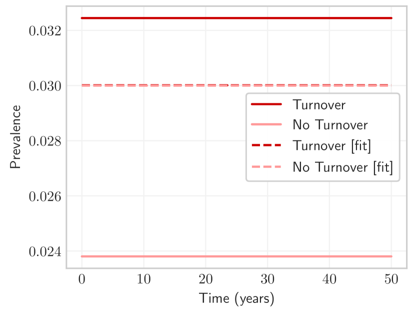
(c) Low risk

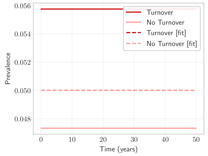
(d) Overall

Figure C.7: Equilibrium STI prevalence among high, medium, and low risk groups as well as overall, with and without turnover, and with and without fitted $C_{i}$ to group-specific prevalence.

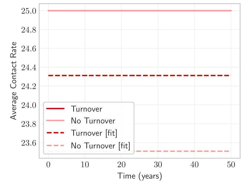
(a) High risk

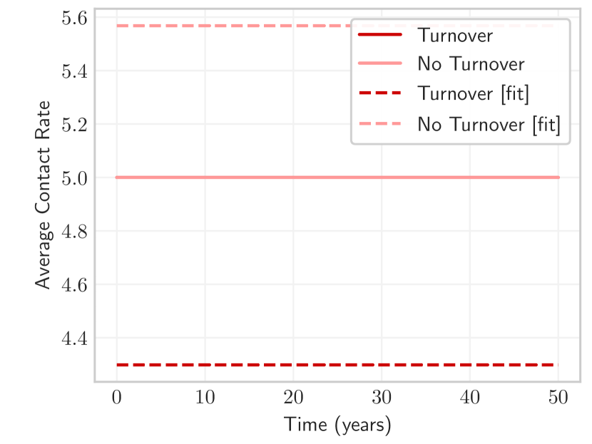
(b) Medium risk

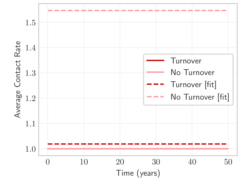
(c) Low risk

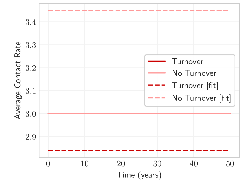
(d) Overall

Figure C.8: Numbers of partners $C_{i}$ among high, medium, and low risk groups as well as overall, with and without turnover, and with and without model fitting to group-specific prevalence.

C.5 Influence of turnover on the tPAF of the highest risk group before model fitting

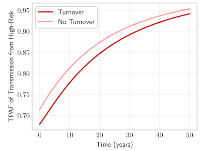
Figure C.9: Transmission population attributable fraction (tPAF) of the high risk group in models with and without turnover, before model fitting.

C.6 Effect of treatment rate on the influence of turnover on equilibrium prevalence

In order to examine the effect of treatment rate $\tau$ on the results of Experiment 1 – the influence of turnover on equilibrium prevalence – we recreated Figures 4 and 7 for a range of treatment rates $\tau\in[0.05,1.0]$. The results are shown in Figure C.10.

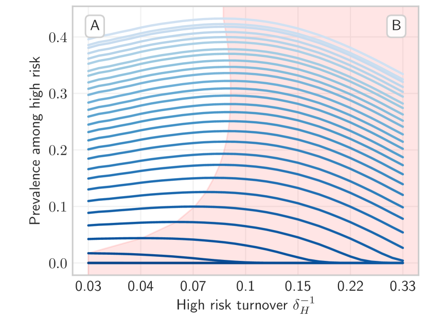
(a) Prevalence among high risk

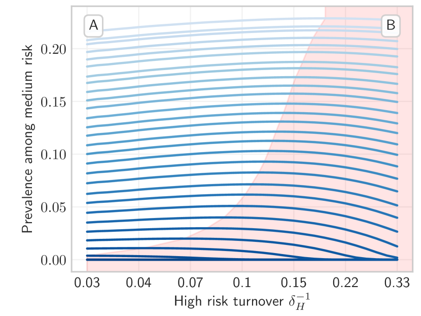
(b) Prevalence among medium risk

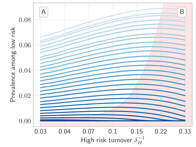
(c) Prevalence among low risk

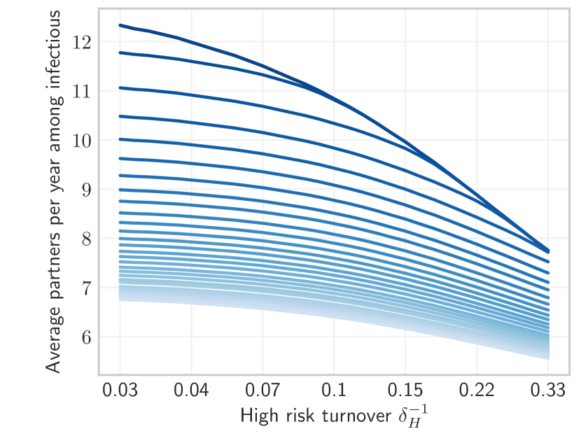
(d) Average $C$ among infectious individuals $\hat{C}_{\mathcal{I}}$

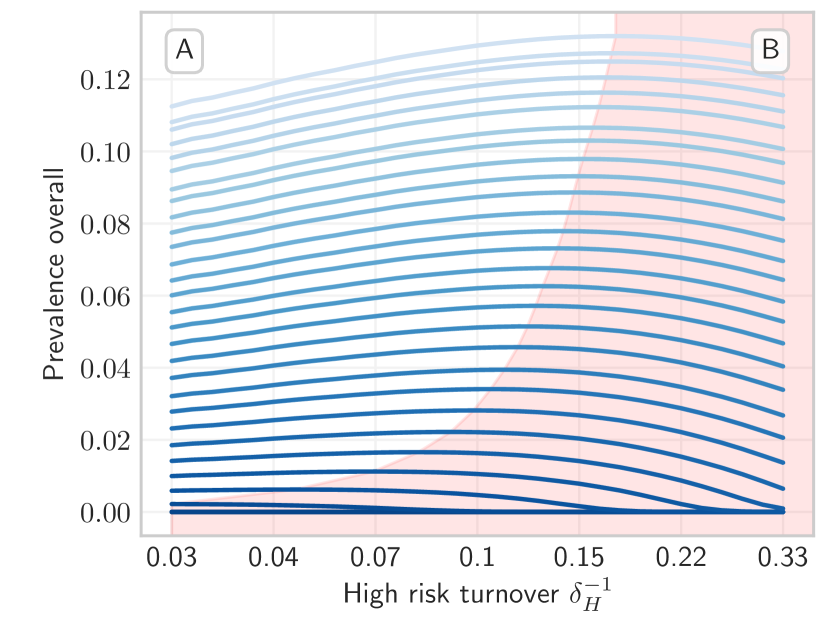
(e) Prevalence overall

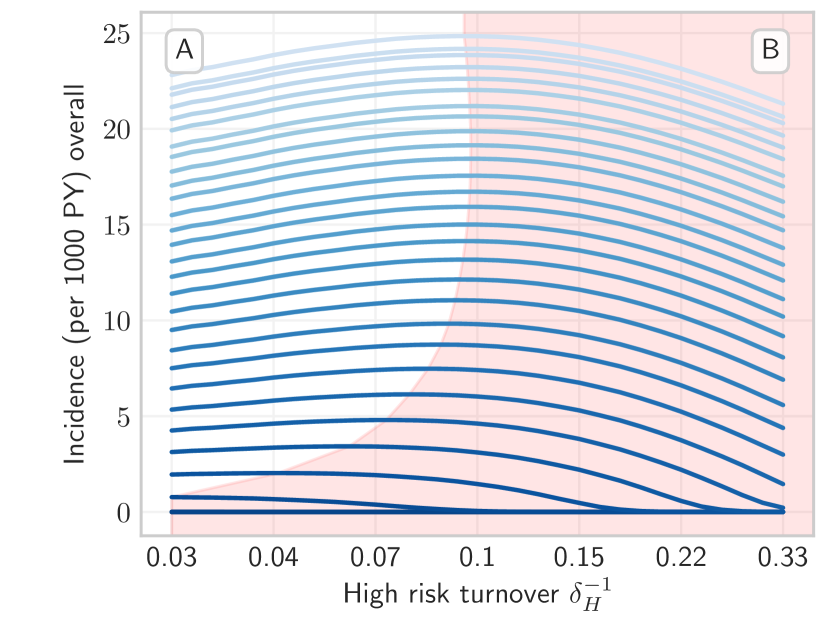
(f) Incidence overall $\lambda$

Figure C.10: Relationship between turnover rate and equilibrium STI prevalence in high, medium, and low risk groups, as well as overall STI prevalence and incidence, and average $C$ among infectious individuals, for a range of treatment rates $\tau$. Darker blue indicates higher treatment rate. The threshold turnover rate separating regions A and B decreases with treatment rate, meaning that increasing turnover becomes more likely to decrease equilibrium prevalence as treatment rate increases.

Turnover rate (log scale) is a function of the duration of time spent in the high risk group $\delta_{H}$, where shorter time spent in the high risk group yields faster turnover. No turnover is indicated by $\delta_{H}^{-1}=0.03$, due to population exit rate $\mu=0.03$.

References

- Abdul-Quader et al. [2014] Abu S Abdul-Quader, Andrew L Baughman, and Wolfgang Hladik. Estimating the size of key populations: Current status and future possibilities. 9(2):107–114, mar 2014. DOI 10.1097/COH.0000000000000041.
- Anderson and May [1991] Roy M Anderson and Robert M May. Infectious diseases of humans: dynamics and control. Infectious diseases of humans: dynamics and control., 1991.
- Baral et al. [2012] Stefan Baral, Chris Beyrer, Kathryn Muessig, Tonia Poteat, Andrea L Wirtz, Michele R Decker, Susan G Sherman, and Deanna Kerrigan. Burden of HIV among female sex workers in low-income and middle-income countries: A systematic review and meta-analysis. The Lancet Infectious Diseases, 12(7):538–549, jul 2012. DOI 10.1016/S1473-3099(12)70066-X. URL https://www.sciencedirect.com/science/article/pii/S147330991270066X?via{%}3Dihub.
- Baral et al. [2013] Stefan Baral, Carmen H Logie, Ashley Grosso, Andrea L Wirtz, and Chris Beyrer. Modified social ecological model: A tool to guide the assessment of the risks and risk contexts of HIV epidemics. BMC Public Health, 13(1):482, may 2013. DOI 10.1186/1471-2458-13-482.
- Baral et al. [2014] Stefan Baral, Sosthenes Ketende, Jessie L. Green, Ping-An An Chen, Ashley Grosso, Bhekie Sithole, Cebisile Ntshangase, Eileen Yam, Deanna Kerrigan, Caitlin E. Kennedy, and Darrin Adams. Reconceptualizing the HIV epidemiology and prevention needs of female sex workers (FSW) in Swaziland. PLoS ONE, 9(12):e115465, dec 2014. DOI 10.1371/journal.pone.0115465.
- Boily and Mâsse [1997] Marie Claude Boily and Benoît Mâsse. Mathematical models of disease transmission: A precious tool for the study of sexually transmitted diseases. Canadian Journal of Public Health, 88(4):255–265, 1997. DOI 10.1007/bf03404793.
- Boily et al. [2015] Marie Claude Boily, Michael Pickles, Michel Alary, Stefan Baral, James Blanchard, Stephen Moses, Peter Vickerman, and Sharmistha Mishra. What really is a concentrated HIV epidemic and what does it mean for West and Central Africa? Insights from mathematical modeling. Journal of Acquired Immune Deficiency Syndromes, 68:S74–S82, mar 2015. DOI 10.1097/QAI.0000000000000437.
- Case et al. [2012] Kelsey Case, Peter Ghys, Eleanor Gouws, Jeffery Eaton, Annick Borquez, John Stover, Paloma Cuchi, Laith Abu-Raddad, Geoffrey Garnett, and Timothy Hallett. Understanding the modes of tranmission model of new HIV infection and its use in prevention planning. Bulletin of the World Health Organization, 90(11):831–838, nov 2012. DOI 10.2471/blt.12.102574.
- Cori et al. [2014] Anne Cori, Helen Ayles, Nulda Beyers, Ab Schaap, Sian Floyd, Kalpana Sabapathy, Jeffrey W. Eaton, Katharina Hauck, Peter Smith, Sam Griffith, Ayana Moore, Deborah Donnell, Sten H. Vermund, Sarah Fidler, Richard Hayes, and Christophe Fraser. HPTN 071 (PopART): A cluster-randomized trial of the population impact of an HIV combination prevention intervention including universal testing and treatment: Mathematical model. PLoS ONE, 9(1):e84511, jan 2014. DOI 10.1371/journal.pone.0084511. URL https://dx.plos.org/10.1371/journal.pone.0084511.
- DataBank [2019] DataBank. Population estimates and projections, 2019. URL https://databank.worldbank.org/source/population-estimates-and-projections.
- Eaton and Hallett [2014] Jeffrey W. Eaton and Timothy B. Hallett. Why the proportion of transmission during early-stage HIV infection does not predict the long-term impact of treatment on HIV incidence. Proceedings of the National Academy of Sciences, 111(45):16202–16207, nov 2014. DOI 10.1073/pnas.1323007111.
- Eaton et al. [2012] Jeffrey W. Eaton, Leigh F. Johnson, Joshua A. Salomon, Till Bärnighausen, Eran Bendavid, Anna Bershteyn, David E. Bloom, Valentina Cambiano, Christophe Fraser, Jan A.C. Hontelez, Salal Humair, Daniel J. Klein, Elisa F. Long, Andrew N. Phillips, Carel Pretorius, John Stover, Edward A. Wenger, Brian G. Williams, and Timothy B. Hallett. HIV treatment as prevention: Systematic comparison of mathematical models of the potential impact of antiretroviral therapy on HIV incidence in South Africa. PLoS Medicine, 9(7):e1001245, jul 2012. DOI 10.1371/journal.pmed.1001245. URL https://dx.plos.org/10.1371/journal.pmed.1001245.
- Fenton et al. [2008] Kevin A. Fenton, Romulus Breban, Raffaele Vardavas, Justin T. Okano, Tara Martin, Sevgi Aral, and Sally Blower. Infectious syphilis in high-income settings in the 21st century. The Lancet Infectious Diseases, 8(4):244–253, apr 2008. DOI 10.1016/S1473-3099(08)70065-3.
- Fergus et al. [2007] Stevenson Fergus, Marc A Zimmerman, and Cleopatra H Caldwell. Growth trajectories of sexual risk behavior in adolescence and young adulthood. American Journal of Public Health, 97(6):1096–1101, jun 2007. DOI 10.2105/AJPH.2005.074609.
- Ganem and Prince [2004] Don Ganem and Alfred M. Prince. Hepatitis B Virus Infection — Natural History and Clinical Consequences. New England Journal of Medicine, 350(11):1118–1129, mar 2004. DOI 10.1056/NEJMra031087.
- Garnett and Anderson [1994] Geoffrey P. Garnett and Roy M. Anderson. Balancing sexual partnership in an age and activity stratified model of HIV transmission in heterosexual populations. Mathematical Medicine and Biology, 11(3):161–192, jan 1994. DOI 10.1093/imammb/11.3.161.
- Hanley [2001] J. A. Hanley. A heuristic approach to the formulas for population attributable fraction. Journal of Epidemiology and Community Health, 55(7):508–514, 2001. DOI 10.1136/jech.55.7.508.
- Henry and Koopman [2015] Christopher J. Henry and James S. Koopman. Strong influence of behavioral dynamics on the ability of testing and treating HIV to stop transmission. Scientific Reports, 5(1):9467, aug 2015. DOI 10.1038/srep09467.
- Hontelez et al. [2013] Jan A.C. C. Hontelez, Mark N. Lurie, Till Bärnighausen, Roel Bakker, Rob Baltussen, Frank Tanser, Timothy B. Hallett, Marie Louise Newell, and Sake J. de Vlas. Elimination of HIV in South Africa through Expanded Access to Antiretroviral Therapy: A Model Comparison Study. PLoS Medicine, 10(10):e1001534, oct 2013. DOI 10.1371/journal.pmed.1001534. URL http://dx.plos.org/10.1371/journal.pmed.1001534.
- ICAP [2019] ICAP. PHIA Project, 2019. URL https://phia.icap.columbia.edu.
- Johnson and Geffen [2016] Leigh F. Johnson and Nathan Geffen. A Comparison of two mathematical modeling frameworks for evaluating sexually transmitted infection epidemiology. Sexually Transmitted Diseases, 43(3):139–146, mar 2016. DOI 10.1097/OLQ.0000000000000412.
- Knight et al. [2019] Jesse Knight, Linwei Wang, Huiting Ma, Sheree Schwartz, Stefan Baral, and Sharmistha Mishra. The influence of risk group turnover in STI/HIV epidemics: mechanistic insights from transmission modeling. In STI & HIV 2019 World Congress, Vancouver, BC, Canada, 2019. URL https://sti.bmj.com/content/95/Suppl_1/A83.3.
- Koopman et al. [1997] J S Koopman, J A Jacquez, G W Welch, C P Simon, B Foxman, S M Pollock, D Barth-Jones, A L Adams, and K Lange. The role of early HIV infection in the spread of HIV through populations. Journal of Acquired Immune Deficiency Syndromes, 14(3):249–58, mar 1997. URL http://www.ncbi.nlm.nih.gov/pubmed/9117458.
- Kraft [1988] Dieter Kraft. A software package for sequential quadratic programming. Technical Report DFVLR-FB 88-28, DLR German Aerospace Center — Institute for Flight Mechanics, Koln, Germany, 1988.
- LAPACK [1992] LAPACK. LAPACK: Linear Algebra PACKage, 1992. URL http://www.netlib.org/lapack.
- Lawson and Hanson [1995] Charles L Lawson and Richard J Hanson. Solving least squares problems, volume 15. SIAM, 1995.
- Maartens et al. [2014] Gary Maartens, Connie Celum, and Sharon R. Lewin. HIV infection: Epidemiology, pathogenesis, treatment, and prevention. The Lancet, 384(9939):258–271, 2014. DOI 10.1016/S0140-6736(14)60164-1.
- Maheu-Giroux et al. [2017] Mathieu Maheu-Giroux, Juan F Vesga, Souleymane Diabaté, Michel Alary, Stefan Baral, Daouda Diouf, Kouamé Abo, and Marie Claude Boily. Changing Dynamics of HIV Transmission in Côte d’Ivoire: Modeling Who Acquired and Transmitted Infections and Estimating the Impact of Past HIV Interventions (1976-2015). Journal of Acquired Immune Deficiency Syndromes, 75(5):517–527, 2017. DOI 10.1097/QAI.0000000000001434.
- Malthus [1798] Thomas Robert Malthus. An Essay on the Principle of Population. 1798.
- Marston and King [2006] Cicely Marston and Eleanor King. Factors that shape young people’s sexual behaviour: a systematic review. Lancet, 368(9547):1581–1586, nov 2006. DOI 10.1016/S0140-6736(06)69662-1.
- May and Anderson [1988] R. M. May and R. M. Anderson. The transmission dynamics of human immunodeficiency virus (HIV)., 1988.
- Mishra et al. [2012] Sharmistha Mishra, Richard Steen, Antonio Gerbase, Ying Ru Lo, and Marie Claude Boily. Impact of High-Risk Sex and Focused Interventions in Heterosexual HIV Epidemics: A Systematic Review of Mathematical Models. PLoS ONE, 7(11):e50691, nov 2012. DOI 10.1371/journal.pone.0050691.
- Mishra et al. [2014] Sharmistha Mishra, Michael Pickles, James F Blanchard, Stephen Moses, and Marie Claude Boily. Distinguishing sources of HIV transmission from the distribution of newly acquired HIV infections: Why is it important for HIV prevention planning? Sexually Transmitted Infections, 90(1):19–25, feb 2014. DOI 10.1136/sextrans-2013-051250.
- Mishra et al. [2016] Sharmistha Mishra, Marie-Claude Boily, Sheree Schwartz, Chris Beyrer, James F. Blanchard, Stephen Moses, Delivette Castor, Nancy Phaswana-Mafuya, Peter Vickerman, Fatou Drame, Michel Alary, and Stefan D. Baral. Data and methods to characterize the role of sex work and to inform sex work programs in generalized HIV epidemics: evidence to challenge assumptions. Annals of Epidemiology, 26(8):557–569, aug 2016. DOI 10.1016/j.annepidem.2016.06.004.
- Mukandavire et al. [2018] Christinah Mukandavire, Josephine Walker, Sheree Schwartz, Marie-Claude Boily, Leon Danon, Carrie Lyons, Daouda Diouf, Ben Liestman, Nafissatou Leye Diouf, Fatou Drame, Karleen Coly, Remy Serge Manzi Muhire, Safiatou Thiam, Papa Amadou Niang Diallo, Coumba Toure Kane, Cheikh Ndour, Erik Volz, Sharmistha Mishra, Stefan Baral, and Peter Vickerman. Estimating the contribution of key populations towards the spread of HIV in Dakar, Senegal. Journal of the International AIDS Society, 21:e25126, jul 2018. DOI 10.1002/jia2.25126.
- Pickles et al. [2013] Michael Pickles, Marie Claude Boily, Peter Vickerman, Catherine M Lowndes, Stephen Moses, James F Blanchard, Kathleen N Deering, Janet Bradley, Banadakoppa M Ramesh, Reynold Washington, Rajatashuvra Adhikary, Mandar Mainkar, Ramesh S Paranjape, and Michel Alary. Assessment of the population-level effectiveness of the Avahan HIV-prevention programme in South India: A preplanned, causal-pathway-based modelling analysis. The Lancet Global Health, 1(5):e289–e299, nov 2013. DOI 10.1016/S2214-109X(13)70083-4.
- Pourbohloul et al. [2003] Babak Pourbohloul, Michael L. Rekart, and Robert C. Brunham. Impact of mass treatment on syphilis transmission: A mathematical modeling approach. Sexually Transmitted Diseases, 30(4):297–305, apr 2003. DOI 10.1097/00007435-200304000-00005.
- Prüss-Ustün et al. [2013] Annette Prüss-Ustün, Jennyfer Wolf, Tim Driscoll, Louisa Degenhardt, Maria Neira, and Jesus Maria Garcia Calleja. HIV Due to Female Sex Work: Regional and Global Estimates. PLoS ONE, 8(5):e63476, 2013. DOI 10.1371/journal.pone.0063476.
- Shubber et al. [2014] Zara Shubber, Sharmistha Mishra, Juan F. Vesga, and Marie Claude Boily. The HIV modes of transmission model: A systematic review of its findings and adherence to guidelines. Journal of the International AIDS Society, 17(1):18928, jan 2014. DOI 10.7448/IAS.17.1.18928.
- Stigum et al. [1994] Hein Stigum, W. Falck, and P. Magnus. The core group revisited: The effect of partner mixing and migration on the spread of gonorrhea, chlamydia, and HIV. Mathematical Biosciences, 120(1):1–23, mar 1994. DOI 10.1016/0025-5564(94)90036-1.
- The DHS Program [2019] The DHS Program. Data, 2019. URL https://www.dhsprogram.com.
- Wasserheit and Aral [1996] J. N. Wasserheit and S. O. Aral. The Dynamic Topology Of Sexually Transmitted Disease Epidemics: Implications For Prevention Strategies. Journal of Infectious Diseases, 174(Supplement 2):S201–S213, oct 1996. DOI 10.1109/ICPDS.2016.7756727. URL https://academic.oup.com/jid/article-lookup/doi/10.1093/infdis/174.Supplement{_}2.S201.
- Watts et al. [2010] C. Watts, C. Zimmerman, A. M. Foss, M. Hossain, A. Cox, and P. Vickerman. Remodelling core group theory: the role of sustaining populations in HIV transmission. Sexually Transmitted Infections, 86(Suppl 3):iii85–iii92, dec 2010. DOI 10.1136/sti.2010.044602.
- Yorke et al. [1978] James A Yorke, Herbert W Hethcote, and Annett Nold. Dynamics and control of the transmission of gonorrhea. Sexually Transmitted Diseases, 5(2):51–56, 1978. DOI 10.1097/00007435-197804000-00003.
- Zhang et al. [2012] Xinyu Zhang, Lin Zhong, Ethan Romero-Severson, Shah Jamal Alam, Christopher J Henry, Erik M Volz, and James S Koopman. Episodic HIV Risk Behavior Can Greatly Amplify HIV Prevalence and the Fraction of Transmissions from Acute HIV Infection. Statistical Communications in Infectious Diseases, 4(1), nov 2012. DOI 10.1515/1948-4690.1041.