Self-consistent quantum field theory for the characterization of complex random media by short laser pulses

Abstract

We present a quantum field theoretical method for the characterization of disordered complex media with short laser pulses in an optical coherence tomography setup (OCT). We solve this scheme of coherent transport in space and time with weighted essentially non-oscillatory methods (WENO). WENO is preferentially used for the determination of highly non-linear and discontinuous processes including interference effects and phase transitions like Anderson localization of light. The theory determines spatio-temporal characteristics of the scattering mean free path and the transmission cross section that are directly measurable in time-of-flight (ToF) and pump-probe experiments. The results are a measure of the coherence of multiple scattering photons in passive as well as in optically soft random media. Our theoretical results of ToF are instructive in spectral regions where material characteristics such as the scattering mean free path and the diffusion coefficient are methodologically almost insensitive to gain or absorption and to higher-order nonlinear effects. Our method is applicable to OCT and other advanced spectroscopy setups including samples of strongly scattering mono- and polydisperse complex nano- and microresonators.

I Introduction

The characterization of disordered media has been fascinating the community ever since, and groundbreaking analysis methods like coherent backscattering (CBS) Akkermans , dynamic light scattering (DLS) Pecora ; Goodman ; Provencher ; Schurtenberger ; Scheffold ; Baravian , diffusing wave spectroscopy (DWS) Pine and optical coherence tomography (OCT) OCT ; Drex ; OCTIEEE ; Zhang ; Zhou ; Dogariu2 have been developed on the basis of transport of classical electromagnetic waves in random media and photonic crystals Akkermans ; John1 ; John2 . Classical methods in the time (TD-OCT) and in the frequency domain (SD-OCT) have been generalized with great success for polarization-sensitive optical coherence tomography deBoer ; Yamanari ; Gosh ; Gompf1 , for applications in metrology Serpo1 ; Serpo2 ; Dogariu ; Gompf as well as for opto-medical imaging Vellekop_Aegerterimaging ; Mosk ; Lippok . Sub- and hyperdiffusive random media Isichenko have attracted great interest. Quantum-optical coherence tomography (QOCT) using entangled-photon-sources in a Hong-Ou-Mandel interferometer Mandel ; Ou has been demonstrated Teich1 ; Teich2 ; Teich3 . It yielded an improvement of the resolution of a factor of two compared to OCT. Probing the submicron scale characteristics of transport of light is a crucial aspect in the understanding of dynamic properties of disordered random media Amon ; Wuensche ; Torres . Many of these approaches however do not account for multiple scattering at all, thus self-interference effects which can yield up to a factor of two enhancement of coherently scattered light with respect to the incoming intensity in passive scatterers ensembles Akkermans , the CBS peak, are neglected. All these methods have in common that a systematic incorporation of multiple scattering processes of light by optically soft scatterers, so the decoherence of light due to light-matter interaction, absorption, all orders of non-linear processes Novitsky as well as scattering losses, are not incorporated in a systematic way Baravian ; Tearney ; Knuttel ; Zvyagin . The range from weakly to strongly scattering non-conserving media so far is not covered by a systematic methodology Alfano ; Nieuwenhuizen ; Rotter2 ; Rotter while quantitative fluorescence spectroscopy (QFS) in the time and the frequency regime is broadly investigated in turbid media and soft matter Mycek . Technological applications in solid state physics and soft matter such as novel light sources, random lasers and solar cells based on multiple scattering in disordered arrangements of active resonators may profit from such novel techniques CaoPNAS ; Chu ; Sun ; Erden . Non-invasive and non-destructive methods of optical analysis and medical imaging that can detect reflected signals as small as $10^{-10}$ of the incident intensity and beyond OCT ; OCTIEEE ; Zhang ; Zhou ; Dogariu2 might be improved again by orders of magnitude. Their application range could be systematically improved in the fields of dynamic and non-conserving media, nematic liquid crystals, semiconductors for telecom applications, glasses and tissue Amon ; Boccara ; Vignolini ; Garcia ; Scheffold2 .
In this article we develop a quantum field theory for photonic transport in dense multiple scattering complex random media, see Fig. 1(a). The Bethe-Salpeter equation, which governs the propagation of the intensity FrankPRB2006 ; Frank2011 , is solved for a propagating short laser pulse in random media with the help of a weighted essentially non-oscillatory solver (WENO) Shu ; Harten ; Osher ; Liu ; Shu2020 ; Lax in the space and time dependent framework Warburton , Fig. 1(c). We are going beyond the diffusion approximation by including interferences and repeated self-interferences in the sense of all orders of maximally crossed diagrams, the Cooperon VW1 ; VW2 . This is generally associated with the Anderson transition of electrons as well as of light, sound and matter waves in multiple scattering random media Anderson ; Chabanov ; PhysicsToday ; Fishman ; SegevChristodoulides ; Genack2 ; Shapiro1 ; Shapiro2 ; SAspect ; Sanchez2019 ; HuS ; Maret2012 ; WS ; NPHOT2013 , and thus with quantum effects VW1 ; VW2 . The random medium is assumed to be optically complex and we are including non-linearities, absorption and gain, which in consequence request the implementation of suitable conservation laws by means of the Ward-Takahashi identity for non-conserving media and resonators. The random medium can be comprised of ensembles of arbitrarily shaped particles as well as correlated disorder and glassy systems in principle Vardeny . We focus in this work on independent non-conserving Mie scatterers Genack ; DUALSYM in strongly scattering ensembles of a high filling fraction, for instance mono- and polydisperse complex TiO₂ powders Evans ; Chakravarthy . Such ensembles are well known for showing a pronounced Mie signature in their transport characteristics such as the scattering mean free path as it has been determined experimentally also by coherent backscattering for optically passive systems Alfano ; Akkermans ; John2 , Fig. 1(d).
We derive in what follows self-consistent results for conserving and for non-conserving random media and we show that absorption and gain or non-linearities can be characterized in a time-of-flight experiment (ToF) by the fraction of transmitted photons which experience a delay due to coherent multiple scattering. It will be shown that the deviation in the long time limit from the pure diffusive case provides fundamental knowledge about the subtle nature of the scattering ensemble and it’s complexity in the sense of the resonator properties of the single scatterer.

Fig1SETUP5.pdf

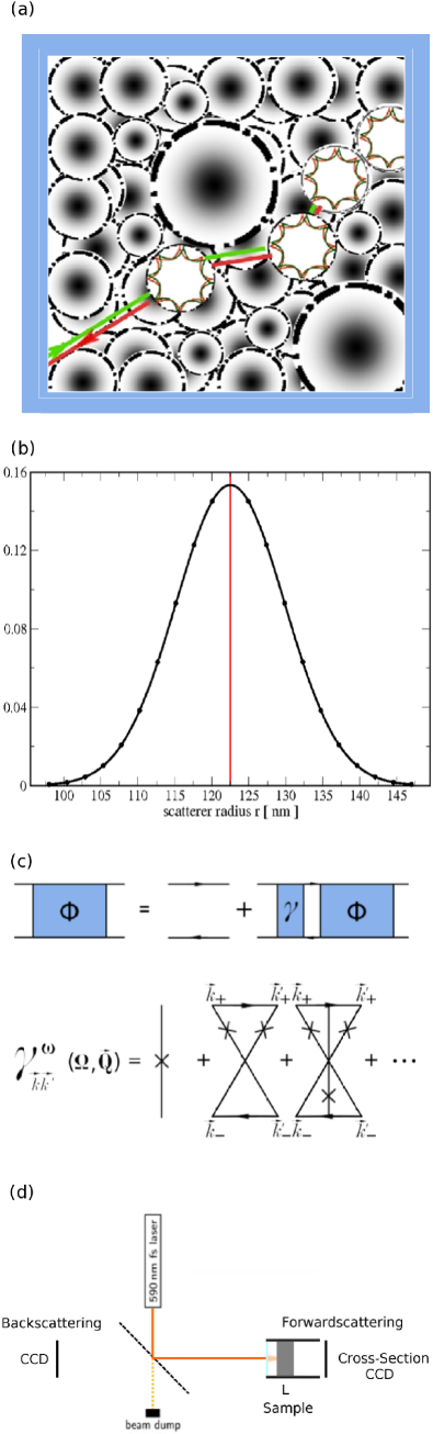
Figure 1: (a) Characterization of disordered random media, mono- and polydisperse Mie scatterers. (b) Gaussian distribution of scatterers radii. (c) Quantum field theoretical approach, self-consistent Bethe-Salpeter equation including the Cooperon. (d) Experimental setup, forward- and backscattering. The discussion is found in the introduction I.

II Quantum field theory for multiple scattering of photons

II.1 Nonlinear response

The electrodynamics for transport of light in random media is described basically by the wave equation

$$\Delta\vec{E}-\frac{1}{c^{2}}\frac{\partial^{2}\vec{E}}{\partial t^{2}}=\frac{1}{c^{2}\epsilon_{0}}\frac{\partial^{2}\vec{P}}{\partial t^{2}}.$$ (1)

where the polarizability in bulk matter $\vec{P}(\vec{E})$ can be decomposed in linear and non-linear part

$$\vec{P} = \epsilon_{0}[\chi^{(1)}\vec{E}+(\chi^{(2)}\vec{E})\vec{E}+((\chi^{(3)}\vec{E})\vec{E})\vec{E}+\,...]$$

$$= \vec{P}_{L}\,+\,\vec{P}_{NL}.$$

As opposed to the non-linear Schrödinger equation for matter waves Sanchez-PLewenstein , in the presented quantum field theoretical formalism the wave equation allows for the straightforward incorporation of the Mie resonance Mie as a classical geometrical effect in the sense of a whispering gallery resonance of the light wave at the inner surface of the complex scatterer Lubatsch05 . In general the polarizability is defined as $\vec{P}(\vec{E})=\epsilon_{0}(\epsilon_{1}-1)\vec{E}+\vec{P}_{NL}$. $\epsilon_{0}$ is the dielectric constant in free space, $\epsilon$ is defined in the literature as the material specific dielectric coefficient $\epsilon\,=\,1\,+\,\chi$, $c$ is the speed of light. Higher-order processes, for instance Kerr media Novitsky with the dielectric susceptibility $\chi^{(2)}$ Evans ; Chakravarthy , are in electrodynamics classified by the dependency of $\vec{P}$ to the electrical field $\vec{E}$ Wegener without loss of generality. It is well known that both the conductivity as well as the susceptibility contribute to the permittivity, so in general ${\rm Im}\epsilon\,=\,{\rm Im}(\chi)\,+\,{\rm Re}(\sigma/\omega)$ is given. Absorption and optical gain are represented by a finite positive or negative imaginary part of the dielectric function, so in general ${\rm Im}\epsilon\neq 0$ is assumed. We take into account the Mie scatterer Fig.(1) for the determination of the single particle self-energy contribution $\Sigma^{\omega}_{\vec{k}}$ of the quantum field-theoretical approach in what follows. The Mie scattering coefficients of n-th order are written as Mie ; Bohren

$$a_{n} = \frac{m\Psi_{n}(my)\Psi_{n}^{\prime}(y)-\Psi_{n}(y)\Psi_{n}^{\prime}(my)}{m\Psi_{n}(my)\xi_{n}^{\prime}(y)-\xi_{n}(y)\Psi_{n}^{\prime}(my)}$$ (3)

$$b_{n} = \frac{\Psi_{n}(my)\Psi_{n}^{\prime}(y)-m\Psi_{n}(y)\Psi_{n}^{\prime}(my)}{\Psi_{n}(my)\xi_{n}^{\prime}(y)-m\xi_{n}(y)\Psi_{n}^{\prime}(my)}.$$

where $m$ here denotes the complex refractive index, $y\,=\,2\pi\,r_{scat}/\lambda$ is the size parameter, $\lambda$ is the wavelength of light and $r_{scat}$ is the spheres radius. Prime denotes the derivative with respect to the argument of the function. $\Psi_{n}$ and $\xi_{n}$ are Riccati-Bessel functions defined in terms of the spherical Bessel function and in terms of the Hankel function Mie ; Bohren . The characteristics of the active scatterer and the active embedding matrix are described by ${\rm Im}\epsilon_{scat}$ and ${\rm Im}\epsilon_{b}$ in the following.

II.2 Self-consistent Bethe-Salpeter equation for inelastic multiple scattering of photons

For the theoretical description we may use any distribution and shape of particles which may be described in the form of a scattering matrix. Here we consider in our results monodisperse spheres as well as a Gaussian distribution of spherical scatterers located at random positions Stoerzer1 ; Stoerzer2 ; Buehrer ; Maret2012 ; WS ; NPHOT2013 ; WiersmaPRL2007 ; WiersmaPRA2008 ; WiersmaLevi2012 ; WiersmaFibonacci2005 ; WiersmaLAGPRE1996 , see Fig. (1). The scatterers and the background medium are described by the dielectric constants $\epsilon_{scat}$ and $\epsilon_{b}$, respectively. In this work we use unpolarized light and therefore we consider the scalar wave equation which has been Fourier transformed from time $t$ to frequency $\omega$ and reads

$$\frac{\omega^{2}}{c^{2}}\,\epsilon(\vec{r}\,)\Psi_{\omega}(\vec{r}\,)+\nabla^{2}\Psi_{\omega}(\vec{r}\,)=-i\omega\frac{4\pi}{c^{2}}j_{\omega}(\vec{r}\,)\ ,$$ (4)

where $c$ denotes the vacuum speed of light and $j_{\omega}(\vec{r}\,)$ the current. The current $j_{\omega}(\vec{r}\,)$ may be expanded in orders of $\omega$ Kubo1 ; Peterson . We do not take into account here a coupling to a microscopic model for dynamical feedback of the optically driven crystal in the non-equilibrium LubatschEPJB ; LubatschSymmetry ; LubatschAPPLSCI2020 , or to chaos modulations and chaotic systems Reichl . The dielectric constant is spatially dependent, $\epsilon(\vec{r}\,)=\epsilon_{b}+\Delta\epsilon\,V(\vec{r}\,)$, and the dielectric contrast is defined as $\Delta\epsilon=\epsilon_{scat}-\epsilon_{b}$. The dielectric contrast describes in principal the arrangement of scatterers through the function $V(\vec{r}\,)=\sum_{\vec{R}}S_{\vec{R}}\,(\vec{r}-\vec{R}\,)$, with $S_{\vec{R}}\,(\vec{r}\,)$ a localized shape function at random locations $\vec{R}$.

The intensity is related to the field-field correlation function $\langle\Psi(\vec{r},\,t\,)\Psi^{*}(\vec{r}\,^{\prime},t\,^{\prime}\,)\rangle$, where angular brackets $\langle\ldots\rangle$ denote the ensemble or disorder average. To calculate the field-field correlation the Green’s function formalism is used, the (single-particle) Green’s function is related to the (scalar) electrical field by

$$\Psi(\vec{r},\,t\,)=\left\lmoustache\!{\rm d}^{3}r\,^{\prime}\right.\!\!\left\lmoustache\!{\rm d}t\,^{\prime}\right.G(\vec{r}\,,\vec{r}\,^{\prime}\,;\,t\,,t^{\prime}\,)j(\vec{r}\,^{\prime}\,,t^{\prime}\,)\,.$$ (5)

The Fourier transform of the retarded, disorder averaged single-particle Green’s function of Eq. (4) reads,

$$G_{\vec{q}}^{\omega}=\frac{1}{\epsilon_{b}(\omega/c)^{2}-|\vec{q}|^{2}-\Sigma^{\omega}_{\vec{q}}}\ ,$$ (6)

where the retarded self-energy $\Sigma_{\vec{q}}^{\omega}$ arises from scattering of the random potential $-(\omega/c)^{2}(\epsilon_{scat}-\epsilon_{b})V(\vec{r}\,)$. Using Green’s functions the mode density, the local density of photonic states (LDOS), $N(\omega)$ may be expressed as $N(\omega)=-(\omega/\pi){\rm Im}G_{0}^{\omega}$, where we use the abbreviation $G_{0}^{\omega}\equiv\int d^{3}q/(2\pi)^{3}\,G_{\vec{q}}^{\omega}$. We study the transport of the already introduced field-field correlation by considering the four-point correlator, defined in terms of the non-averaged Green’s functions $\hat{G}$, $\hat{G}^{*}$ in momentum and frequency space as $\Phi^{\omega}_{\vec{q}\vec{q}^{\prime}\,\,}(\vec{Q},\Omega)=\langle\hat{G}^{\omega_{+}}_{{\vec{q}}_{+}{\vec{q}}_{+}^{\,\prime}}\hat{G}^{\omega_{-}\,*}_{{\vec{q}}_{-}^{\,\prime}{\vec{q}}_{-}}\rangle$. Here we introduced Lubatsch05 the center-of-mass and the relative frequencies ($\Omega$, $\omega$) and momenta ($\vec{Q}$, $\vec{q}$) with $\omega_{1,2}\,=\,\omega\pm\Omega/2$ and $\vec{q}_{1,2}\,=\,\vec{q}\pm\vec{Q}/2$. The variables $\Omega$, $\vec{Q}$ are associated with the time and the position dependence of the averaged energy density, with $\hat{Q}=\vec{Q}/|\vec{Q}|$, while $\omega_{\pm}=\omega\pm\Omega/2$ and $\vec{q}_{\pm}=\vec{q}\pm\vec{Q}/2$ etc. are the frequencies and momenta of in- and out-going waves, respectively. The intensity correlation, the disorder averaged particle-hole Green’s function, $\Phi^{\omega}_{\vec{q}\vec{q}^{\prime}}(\vec{Q},\Omega)$ is described by the Bethe-Salpeter equation

$$\!\!\!\!\!\!\!\!\!\!\!\!\!\!\!\!\!\!\!\!\!\!\!\!\!\!\!\!\!\!\!\!\!\!\!\!\Phi_{\vec{q}\vec{q}^{\prime}}\,=\,G^{R}_{q_{+}}(\omega_{+})G^{A}_{q_{-}}(\omega_{-}){\color[rgb]{1,1,1}0000000000000000}$$

$$\!\qquad{\color[rgb]{1,1,1}00000000}\left[\delta(\vec{q}-\vec{q}\prime)+\left\lmoustache\frac{{\rm d}^{3}q\,^{\prime\prime}\,}{(2\pi)^{3}}\right.\gamma_{q\,q\,^{\prime\prime}\,}\Phi_{\vec{q}\,^{\prime\prime}\,\vec{q}\,^{\prime}\,}\right]\,.$$ (7)

By utilizing the averaged single particle Green’s function, c.f. Eq. (6), on the left-hand side of Eq. (II.2) the Bethe-Salpeter equation may be rewritten as the kinetic equation, see, e.g., ref. Lubatsch05 ,

$$\left[\omega\Omega\frac{{\rm Re}{\epsilon_{b}}}{c^{2}}-Q\,(\vec{q}\cdot\hat{Q})+\frac{i}{c^{2}\tau^{2}}\right]\Phi^{\omega}_{\vec{q}\vec{q}^{\prime}} =$$ (8)

$$-i{\rm Im}G^{\omega}_{\vec{q}}\left[\delta(\vec{q}-\vec{q}\prime)+\left\lmoustache\frac{{\rm d}^{3}q^{\prime\prime}}{(2\pi)^{3}}\right.\gamma^{\omega}_{\vec{q}{\vec{q}^{\prime\prime}}}\Phi^{\omega}_{\vec{q}^{\prime\prime}\vec{q}^{\prime}}\right].$$

When we analyze the correlation function’s long-time ($\Omega\to 0$) and long-distance ($|\vec{Q}|\to 0$) behavior, terms of $O(\Omega^{2},Q^{3},\Omega Q)$ are neglected. Eq. (8) contains the total quadratic momentum relaxation rate $1/\tau^{2}=c^{2}\,{\rm Im}(\epsilon_{b}\omega^{2}/c^{2}-\Sigma^{\omega})$ due to absorption/gain and due to impurity scattering in the background medium as well as the irreducible two-particle vertex function $\gamma^{\omega}_{\vec{q}\vec{q}^{\,\prime}}(\vec{Q},\Omega)$. In order to solve this equation we expand it into moments.

The energy conservation is implemented in the solution of the Bethe-Salpeter equation by a Ward identity (WI) for the photonic case, see Ref. Lubatsch05 . The Ward identity is derived in the generalized form for the scattering of photons in non-conserving media. Non-linear effects, absorption and gain yield an additional contribution, and a form of the Ward-Takahashi identity for photons in complex matter Lubatsch05 ; WARD ; TAKAHASHI is derived. The additional contribution is not negligible and thus effectively present in all results of the transport characteristics of the self-consistent framework Lubatsch05 ; FrankPRB2006 ; Frank2011 . For scalar waves the Ward identity assumes the following exact form

$$\Sigma^{\omega_{+}}_{\vec{q}_{+}}-\Sigma^{\omega_{-}\,*}_{\vec{q}_{-}}\!\! - \!\!\left\lmoustache\!\!\frac{{\rm d}^{3}q^{\prime}}{(2\pi)^{3}}\right.\left[G^{\omega_{+}}_{{\vec{q}}_{+}^{\,\prime}}-G^{\omega_{-}\,*}_{{\vec{q}}_{-}^{\,\prime}}\right]\,{\gamma}^{\omega}_{{\vec{q}}^{\,\prime}{{\vec{q}}}}({\vec{Q}},\Omega)$$

$$= \!\!\!f_{\omega}(\Omega)\!\left[\!{\rm Re}{\Sigma}^{\omega}_{{\vec{q}}}\!+\!\!\left\lmoustache\!\!\frac{\rm d^{3}q^{\prime}}{(2\pi)^{3}}\right.{\rm Re}{G}^{\omega}_{{\vec{q}}^{\,\prime}}\,{\gamma}^{\omega}_{{\vec{q}}^{\,\prime}{{\vec{q}}}}({\vec{Q}},\Omega)\right]\!.$$

The right-hand side of Eq. (II.2) represents reactive effects (real parts), originating from the explicit $\omega^{2}$-dependence of the photonic random potential. In conserving media (${\rm Im}\epsilon_{b}={\rm Im}\epsilon_{scat}=0$) these terms renormalize the energy transport velocity $v_{\mbox{\tiny E}}$ relative to the average phase velocity $c_{p}$ without emphasizing the diffusive long-time behavior.Kroha ; Lubatsch05 In presence of loss or gain, additional effects are enhanced by the prefactor

$$f_{\omega}(\Omega)=\frac{(\omega\Omega{\rm Re}\Delta\epsilon+i\omega^{2}{\rm Im}\Delta\epsilon)}{(\omega^{2}{\rm Re}\Delta\epsilon+i\omega\Omega{\rm Im}\Delta\epsilon)},$$ (10)

which now does not vanish in the limit of $\Omega\to 0$.

II.3 Expansion of the two-particle Green’s function into moments

The solution of the Bethe-Salpeter equation is derived by rewriting it in the form of a kinetic equation and by deriving a continuity equation. For this aim we expand the intensity correlator into its moments and we extract a diffusion pole structure from the Bethe-Salpeter equation Eq. (II.2). The $\vec{q}\,^{\prime}\,$ integrated correlator

$$\Phi_{\vec{q}}=\left\lmoustache\!\!\frac{{\rm d}^{3}q\,^{\prime}\,}{(2\pi)^{3}}\right.\!\!\Phi_{\vec{q\,}\vec{q}\,^{\prime}\,}$$ (11)

is decoupled from the momentum dependent prefactors by some auxiliary approximation scheme. This approximation must obey the results of the ladder approximation and it must incorporate the set of physical relevant variables for the observed phenomena. In a first step we use the bare first two moments of the correlation function $\Phi_{\vec{q}}$ defined as

$$\Phi_{\rho\rho}(\vec{Q},\Omega) = \left\lmoustache\!\frac{{\rm d}^{3}q}{(2\pi)^{3}}\right.\!\!\left\lmoustache\!\frac{{\rm d}^{3}q\,^{\prime}}{(2\pi)^{3}}\right.\Phi_{\vec{q}\,\vec{q}\,^{\prime}\,}$$ (12)

$$\Phi_{j\rho}(\vec{Q},\Omega) = \left\lmoustache\!\frac{{\rm d}^{3}q}{(2\pi)^{3}}\right.\!\!\left\lmoustache\!\frac{{\rm d}^{3}q\,^{\prime}}{(2\pi)^{3}}\right.(\vec{q}\cdot\hat{Q})\Phi_{\vec{q}\,\vec{q}\,^{\prime}\,}.$$ (13)

These bare moments are related to physical quantities, the energy density correlation $P^{\omega}_{\mbox{\tiny E}}(\vec{Q},\Omega)$ and the current density correlation $J^{\omega}_{\mbox{\tiny E}}(\vec{Q},\Omega)$, by dimensional prefactors:

$$P^{\omega}_{\mbox{\tiny E}}(\!\vec{Q},\Omega)\!\! = \!\!\left[\!\frac{\omega}{c_{\mbox{\tiny p}}}\!\right]^{2}\!\!\!\Phi_{\rho\rho}\,\,\,\,\Leftrightarrow\Phi_{\rho\rho}\!=\!\left[\!\frac{c_{\mbox{\tiny p}}}{\omega}\!\right]^{2}\!\!P^{\omega}_{\mbox{\tiny E}}(\!\vec{Q},\Omega)$$ (14)

$$J^{\omega}_{\mbox{\tiny E}}(\!\vec{Q},\Omega)\!\! = \!\!\left[\!\frac{\omega v_{\mbox{\tiny E}}}{c_{\mbox{\tiny p}}}\!\right]\!\Phi_{j\rho}\Leftrightarrow\Phi_{j\rho}\!=\!\left[\!\frac{c_{\mbox{\tiny p}}}{\omega v_{\mbox{\tiny E}}}\!\right]\!J^{\omega}_{\mbox{\tiny E}}(\!\vec{Q},\Omega)\,.$$ (15)

The projection of the correlator $\Phi_{\vec{q}}$, Eq. (11), onto the bare moments $\Phi_{\rho\rho}(\vec{q},\Omega)$ as in Eq. (12), and $\Phi_{j\rho}(\vec{q},\Omega)$, as in Eq. (13), is therefore then by

$$\left\lmoustache\!\frac{{\rm d}^{3}q\,^{\prime}}{(2\pi)^{3}}\Phi_{\vec{q}\vec{q}\,^{\prime}}\right. \!\!=\!\! \frac{A(\vec{q}\,)}{\!\left\lmoustache\!\!\frac{{\rm d}^{3}q^{\prime}}{(2\pi)^{3}}\right.\!\!A(\vec{q}\,^{\prime})}\Phi_{\rho\rho}(\vec{Q},\Omega)$$

$$\!\!+\!\! \frac{B(\vec{q}\,)(\vec{q}\cdot\hat{Q})}{\!\left\lmoustache\!\!\frac{{\rm d}^{3}q^{\prime}}{(2\pi)^{3}}\right.\!\!B(\vec{q}\,^{\prime})(\vec{q}\,^{\prime}\cdot\hat{Q})^{2}}\Phi_{j\rho}(\vec{Q},\Omega).$$

The projection coefficients $A(\vec{q}\,)$ and $B(\vec{q}\,)$ are to be determined in the following. In this expansion the bare moments may be substituted by their physical counterparts, the energy density $P^{\omega}_{\mbox{\tiny E}}$ in Eq. (14) and the current density $J^{\omega}_{\mbox{\tiny E}}(\vec{Q},\Omega)$ from Eq. (15). The expansion coefficients $A(\vec{q}\,)$ and $B(\vec{q}\,)$ in Eq. (II.3) behave uncritically when the system localizes. Thus they can be determined by using the simple ladder approximation, where all expressions are known exactly. The ladder approximation of the two-particle vertex function is schematically explained in Lubatsch05 ; FrankPRB2006 ; Frank2011 .

In the following we use the approximation to obtain the expansion coefficients from it. In the ladder approximation the zeroth bare moment is given by

$$\Phi_{\rho\rho}^{L}(\vec{Q},\Omega) = \left\lmoustache\!\frac{{\rm d}^{3}q}{(2\pi)^{3}}\right.\!\!\left[G_{\vec{q}_{+}}(\vec{Q},\Omega)G^{*}_{\vec{q}_{-}}(\vec{Q},\Omega)\right]^{2}\Gamma_{L}$$ (17)

$$= \frac{1}{\tilde{\gamma}_{0}^{2}}\Gamma_{L},$$

the superscript $L$ refers to the ladder approximation. The product $\left\lmoustache\!\frac{{\rm d}^{3}q}{(2\pi)^{3}}\right.\!\!\left[G_{\vec{q}_{+}}(\vec{Q},\Omega)G^{*}_{\vec{q}_{-}}(\vec{Q},\Omega)\right]^{2}$ has been expanded up to linear order in $\vec{q}$. The renormalized vertex $\tilde{\gamma}_{0}$ is given by

$$\tilde{\gamma}_{0} \!\!=\!\! \gamma_{0}\!+\!f_{\omega}(\Omega)\frac{\left(\!{\rm Re\,}\gamma_{0}G_{0}\!+\!{\rm Re\,}\Sigma\!\right)}{{\rm Im\,}G_{0}}\!-\!\frac{\omega^{2}{\rm Im\,}\epsilon_{b}}{{\rm Im\,}G_{0}}$$ (18)

where $\gamma_{0}$ is the bare vertex. $f_{\omega}(\Omega)$ is arising from the Ward identity and has been defined in Eq. (II.2). Within the simple ladder approximation the bare moment $\Phi^{L}_{j\rho}(\vec{Q},\Omega)$ defined in Eq. (13) is thus given by

$$\Phi^{L}_{j\rho}(\!\vec{Q},\Omega)\!\!=\!\!\!\left\lmoustache\!\frac{{\rm d}^{3}q}{(2\pi)^{3}}\right.\!\!(\vec{q}\cdot\hat{Q})G_{\vec{q}_{+}}\!G^{*}_{\vec{q}_{-}}\!\!\left\lmoustache\!\frac{{\rm d}^{3}q\,^{\prime}\,}{(2\pi)^{3}}\right.\!\!G_{\vec{q}\,^{\prime}_{+}}\!G^{*}_{\vec{q}\,^{\prime}_{-}}\!\!\Gamma_{L}\,.$$ (19)

We follow this strategy again and by expanding the product $G_{\vec{q}\,^{\prime}_{+}}G^{*}_{\vec{q}\,^{\prime}_{-}}$ under the second integral up to first order in $\vec{q\,}^{\prime}$ we obtain the expression

$$\Phi^{L}_{j\rho}(\vec{Q},\Omega)=\frac{1}{\tilde{\gamma}_{0}}\Gamma_{L}\!\left\lmoustache\!\frac{{\rm d}^{3}q}{(2\pi)^{3}}\right.\!\!(\vec{q}\cdot\hat{Q})G_{\vec{q}_{+}}G^{*}_{\vec{q}_{-}}$$ (20)

By employing the same expansion to the remaining product of the Green’s function one eventually finds

$$\Phi^{L}_{j\rho}(\vec{Q},\Omega)=\frac{\Gamma_{L}}{\tilde{\gamma}_{0}}\!\left\lmoustache\!\frac{{\rm d}^{3}q}{(2\pi)^{3}}\right.\!\!(\vec{q}\cdot\hat{Q})\frac{1}{2}\frac{\Delta G_{\vec{q}}^{2}(\vec{q}\cdot\hat{Q})Q}{\tilde{\gamma}_{0}\Delta G_{0}},$$ (21)

where the abbreviation $\Delta G\equiv G-G^{*}$ has been introduced.

In the next step of determining the expansion coefficients $A(\vec{q}\,)$ and $B(\vec{q}\,)$, Eq. (II.3), we go back to the field-field correlation function $\Phi_{\vec{q}\vec{q}\,^{\prime}\,}$. In the uncritical ladder approximation the two particle Green’s function is given by

$$\!\left\lmoustache\!\frac{{\rm d}^{3}q\,^{\prime}}{(2\pi)^{3}}\right.\!\!\Phi_{\vec{q}\vec{q}\,^{\prime}}=\left[G_{\vec{q}_{+}}G^{*}_{\vec{q}_{-}}\right]\Gamma_{L}\!\left\lmoustache\!\frac{{\rm d}^{3}q\,^{\prime}}{(2\pi)^{3}}\right.\!\!G_{\vec{q}\,^{\prime}_{+}}G^{*}_{\vec{q}\,^{\prime}_{-}}.$$ (22)

Employing the momentum expansion again, the equation, Eq. (22) can be simplified to yield

$$\Phi_{\vec{q}}=\frac{\Delta G_{\vec{q}}}{\tilde{\gamma}_{0}^{2}\Delta G_{0}}\Gamma_{L}+\frac{1}{2}\frac{\Delta G_{\vec{q}}^{2}(\vec{q}\cdot\hat{Q})Q}{\tilde{\gamma}_{0}^{2}\Delta G_{0}}\Gamma_{L}.$$ (23)

By using the above given momentum expansion, Eq. (23), in combination with the expressions given in Eq. (21) and in Eq. (17) in connection with the described projection, or expansion into moments, Eq. (II.3), the following relation is eventually derived

$$\frac{\Delta G_{\vec{q}}}{\tilde{\gamma}_{0}^{2}\Delta G_{0}}\Gamma_{L}+\frac{1}{2}\frac{\Delta G_{\vec{q}}^{2}(\vec{q}\cdot\hat{Q})Q}{\tilde{\gamma}_{0}^{2}\Delta G_{0}}\Gamma_{L}$$ (24)

$$=\!\frac{A(\vec{q}\,)}{\!\left\lmoustache\!\!\frac{{\rm d}^{3}q^{\prime}}{(2\pi)^{3}}\right.\!\!A(\vec{q}\,^{\prime})}\frac{1}{\tilde{\gamma}_{0}^{2}}\Gamma_{L}$$

$$+\frac{B(\vec{q}\,)(\vec{q}\cdot\hat{Q})}{\!\left\lmoustache\!\!\frac{{\rm d}^{3}q^{\prime}}{(2\pi)^{3}}\right.\!\!B(\vec{q}\,^{\prime})(\vec{q}\,^{\prime}\cdot\hat{Q})^{2}}\frac{\Gamma_{L}}{\tilde{\gamma}_{0}}\!\left\lmoustache\!\frac{{\rm d}^{3}q}{(2\pi)^{3}}\right.\!\!(\vec{q}\cdot\hat{Q})\frac{1}{2}\frac{\Delta G_{\vec{q}}^{2}(\vec{q}\cdot\hat{Q})Q}{\tilde{\gamma}_{0}\Delta G_{0}}\,.$$

By comparison of coefficients in the relation, Eq. (24), the demanded coefficients $A({\vec{q}}\,)$ and $B({\vec{q}}\,)$ of the expansion into moments, Eq. (II.3), can now be determined as follows

$$A({\vec{q}}\,)=\Delta G_{\vec{q}}\qquad B({\vec{q}}\,)=\Delta G_{\vec{q}}^{2}.$$ (25)

Employing those expressions for the expansion coefficients, we can eventually express the two-particle correlator $\Phi_{\vec{q}\vec{q}\,^{\prime}}$ as follows

$$\!\left\lmoustache\!\frac{{\rm d}^{3}q^{\prime}}{(2\pi)^{3}}\right.\!\!\Phi_{\vec{q}\vec{q}\,^{\prime}} = \frac{\Delta G_{\vec{q}}}{\left(\frac{\omega}{c_{\mbox{\tiny p}}}\right)^{2}\!\left\lmoustache\!\!\frac{{\rm d}^{3}q\,^{\prime}}{(2\pi)^{3}}\right.\!\!\Delta G_{\vec{q}\,^{\prime}}}P^{\omega}_{\mbox{\tiny E}}(\vec{Q},\Omega)$$

$$+\frac{\Delta G_{\vec{q}}^{2}(\vec{q}\cdot\hat{Q})}{\left(\frac{\omega v_{\mbox{\tiny E}}}{c_{\mbox{\tiny p}}}\right)\!\left\lmoustache\!\!\frac{{\rm d}^{3}q\,^{\prime}}{(2\pi)^{3}}\right.\!\!\Delta G_{\vec{q}\,^{\prime}}^{2}(\vec{q}\,^{\prime}\cdot\hat{Q})^{2}}J^{\omega}_{\mbox{\tiny E}}(\vec{Q},\Omega).$$

The expression, Eq. (II.3), represents the complete expansion of the intensity correlator into its moments. This form is used now to decouple and therefore solve the Bethe-Salpeter equation.

II.4 General solution of the Bethe-Salpeter equation

We repeat the most important steps so far. The disorder averaged intensity correlation, the two-particle Green’s function, obeys the Bethe-Salpeter equation, see Eq. (II.2)

$$\Phi_{\vec{q}\,\vec{q}\,^{\prime}\,}\!\! = \!\!G_{q_{+}}^{\omega_{+}}G^{*\,\omega_{-}}_{q_{-}}\!\left[1\!\!+\!\!\!\left\lmoustache\!\!\frac{{\rm d}^{3}q\,^{\prime\prime}\,}{(2\pi)^{3}}\right.\!\!\gamma_{q\,q\,^{\prime\prime}\,}\Phi_{\vec{q}\,^{\prime\prime}\,\vec{q}\,^{\prime}}\right]$$ (27)

The Bethe-Salpeter equation may be rewritten into the kinetic or Boltzmann equation given in Eq. (8)

$$\!\!\!\!\!\!\!\!\!\!\!\!\!\!\!\!\!\!\!\left[(\omega\Omega)\,2{\rm Re\,}\epsilon-Q\left(\vec{q}\cdot\hat{Q}\right)+\Delta\Sigma-\omega^{2}\Delta\epsilon\right]\Phi_{\vec{q}}$$

$$\qquad=\Delta G_{\vec{q}}+\left\lmoustache\!\!\frac{{\rm d}^{3}q\,^{\prime}}{(2\pi)^{3}}\right.\!\!\Delta G_{\vec{q}}\gamma_{\vec{q}\vec{q}\,^{\prime}\,}\Phi_{\vec{q}\,^{\prime}\,}\,.$$ (28)

To find the solution of Eq. (II.4), we first sum in Eq. (II.4) over momenta $\vec{q}$, and we incorporate the generalized Ward identity as given in Eq. (II.2) and we expand the obtained result for small internal momenta $Q$ and internal frequencies $\Omega$. It is essential to employ the form of the two-particle correlator shown in Eq. (II.3). Eventually the generalized continuity equation for the energy density can be derived as

$$\Omega P^{\omega}_{\mbox{\tiny E}}+QJ^{\omega}_{\mbox{\tiny E}}=\frac{4\pi i\,\omega\,N(\omega)}{g^{(1)}_{\omega}\left[1+\Delta(\omega)\right]c_{p}^{2}}\!\! + \!\!\frac{i[g^{(0)}_{\omega}+\Lambda(\omega)]}{g^{(1)}_{\omega}\left[1+\Delta(\omega)\right]}P^{\omega}_{\mbox{\tiny E}}.$$

The generalized continuity equation represents energy conservation in the presence of optical gain and/or absorption.

As the standard solution procedure the next step is to obtain a linearly independent equation which relates the energy density $P^{\omega}_{\mbox{\tiny E}}$ and the current density $J^{\omega}_{\mbox{\tiny E}}$. This is realized in a similar way to above, one first multiplies the kinetic equation, Eq.(II.4), by the projector $\left[\vec{q}\cdot\hat{Q}\right]$ and then follows the already outlined steps to eventually obtain the wanted second relation. This is the current relaxation equation

$$\left[\omega\Omega\frac{{\rm Re}{\epsilon_{b}}}{c^{2}}+\frac{i}{c^{2}\tau^{2}}+iM(\Omega)\right]J^{\omega}_{\mbox{\tiny E}}\!\! + \!\!\tilde{A}\,QP_{\mbox{\tiny E}}^{\omega}=0\ ,$$ (30)

relating the energy density $P^{\omega}_{\mbox{\tiny E}}$ and the energy density current $J^{\omega}_{\mbox{\tiny E}}$. The memory function $M(\Omega)$ is introduced according to

$$M\!(\Omega)\!=\!\frac{i\!\!\left\lmoustache\!\!\frac{{\rm d}^{3}q}{(2\pi)^{3}}\right.\!\!\!\left\lmoustache\!\!\frac{{\rm d}^{3}q\,^{\prime}}{(2\pi)^{3}}\right.\!\![\vec{q}\!\cdot\!\hat{Q}]\Delta G_{\vec{q}}^{\omega}\gamma^{\omega}_{\vec{q}\vec{q}\,^{\prime}}(\Delta G_{\vec{q}\,^{\prime}}^{\omega})^{2}[\vec{q}\,^{\prime}\!\cdot\!\hat{Q}]}{\left\lmoustache\!\!\frac{{\rm d}^{3}q}{(2\pi)^{3}}\right.[\vec{q}\!\cdot\!\hat{Q}]^{2}(\Delta G_{\vec{q}}^{\omega})^{2}},$$ (31)

where $\gamma^{\omega}_{\vec{p}\vec{p}^{\prime}}\equiv\gamma^{\omega}_{\vec{p}\vec{p}^{\prime}}(\vec{Q},\Omega)$ is the total irreducible two-particle vertex, which will be discussed in detail in what follows.

So far, two independent equations, Eq. (LABEL:continuityL) and Eq. (30), have been obtained. Either of them is relating the current density $J^{\omega}_{\mbox{\tiny E}}$ with the energy density $P^{\omega}_{\mbox{\tiny E}}$. Now one can eliminate one of the two variables in this linear system of equations. The two equation are combined to find an expression for the energy density

$$P_{\mbox{\tiny E}}^{\omega}(Q,\Omega)=\frac{4\pi iN(\omega)/(g^{(1)}_{\omega}\left[1+\Delta(\omega)\right]c_{p}^{2})}{\Omega+iQ^{2}D+i\xi_{a}^{-2}D}\ ,$$ (32)

that exhibits the expected diffusion pole structure for non-conserving media. Precisely in the denominator of Eq. (32) there appears an additional term as compared to the case of conserving media. This is the term $\xi_{a}^{-2}D$, the mass term, accounting for loss (or gain) to the intensity not being due to diffusive relaxation. In Eq. (32) also the generalized, $\Omega$-dependent diffusion coefficient $D(\Omega)$ has been introduced by the relation

$$D(\Omega)\left[1-i\,\Omega\omega\tau^{2}{\rm Re}\epsilon_{b}\right]=D_{0}^{tot}-c^{2}\tau^{2}D(\Omega)M(\omega).$$ (33)

It shall be noted that Eq. (32) introduces the absorption or gain induced growth or absorption scale $\xi_{a}$ of the diffusive modes,

$$\xi_{a}^{-2} = \frac{r_{\epsilon}A_{\epsilon}-2\omega^{2}{\rm Im}\epsilon_{b}}{2{\rm Re}\epsilon_{b}-A_{\epsilon}B_{\epsilon}/\omega}\ \frac{1}{\omega D(\Omega)},$$ (34)

which is to be well distinguished from the single-particle or amplitude absorption or amplification length. The diffusion constant without memory effects in Eq. (33), $D_{0}^{tot}=D_{0}+D_{b}+D_{scat}$, consists of the bare diffusion constant Kroha ,

$$D_{0}=\frac{2v_{\mbox{\tiny E}}c_{p}}{\pi N(\omega)}\left\lmoustache\!\!\frac{{\rm d}^{3}q}{(2\pi)^{3}}\right.[\vec{q}\cdot\hat{Q}]^{2}({\rm Im}G_{\vec{q}}^{\omega})^{2}$$ (35)

and renormalizations from absorption or gain in the background medium ($D_{b}$) and in the scatterers ($D_{scat}$),

$$D_{b}=\left(\omega\tau\right)^{2}\,{\rm Im}\epsilon_{b}\,\tilde{D}_{0}/4\ ,\quad D_{scat}=r_{\epsilon}A_{\epsilon}\tau^{2}\tilde{D}_{0}/8\ ,$$ (36)

where $\tilde{D}_{0}$ is the same as in Eq. (35), with $\Delta G(Q,\Omega)=(G_{\vec{q}}^{\omega})^{A}-(G_{\vec{q}}^{\omega})^{R}$ replaced by $\Box G(Q,\Omega)=(G_{\vec{q}}^{\omega})^{A}+(G_{\vec{q}}^{\omega})^{R}$ FrankPRB2006 ; Frank2011 ; ApplSci , and $({\rm Im}G_{\vec{q}}^{\omega})^{2}$ replaced by ${(\rm Re}G_{\vec{q}}^{\omega})^{2}$, respectively. In the above Eqs. (34)-(36) the following short-hand notations have been introduced,

$$u_{\epsilon} = \frac{{\rm Im}(\Delta\epsilon\Sigma^{\omega})}{{\rm Im}(\Delta\epsilon G_{0}^{\omega})}\ ,\qquad\qquad r_{\epsilon}={{\rm Im}\Delta\epsilon}/{{\rm Re}\Delta\epsilon},$$

$$A_{\epsilon} = 2[u_{\epsilon}{\rm Re}G_{o}+{\rm Re}\Sigma_{o}]$$

$$B_{\epsilon} = \frac{({\rm Re}\Delta\epsilon)^{2}+({\rm Im}\Delta\epsilon)^{2}}{2\omega^{2}({\rm Re}\Delta\epsilon)^{2}}.$$

II.5 Vertex function and self-consistency

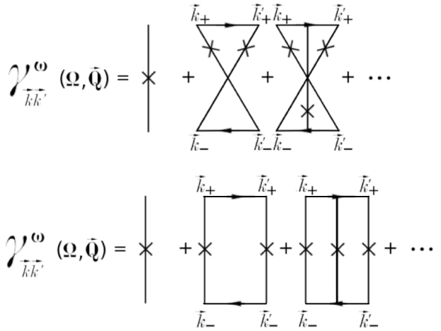
Figure 2: The upper panel shows a diagrammatic expansion of the irreducible two-particle vertex $\gamma$. The bottom panel displays the disentangled Cooperon with changed momentum arguments.

According to Eq. (31) and Eq. (33) the energy density, the two-particle function, given in Eq. (32) still depends on the full two-particle vertex $\gamma^{\omega}_{{\vec{q}}^{\,\prime}{{\vec{q}}}}$. Before discussing the vertex function, we briefly recall our arguments with regards to dissipation. Dissipation breaks the time reversal symmetry OnsagerI ; OnsagerII on the one hand side but on the other hand the dissipation rate itself is invariant under time reversal. As a general picture of this physics the damped harmonic oscillator can be mentioned, where the time reversed solution is still damped with the very same damping constant. Having this in mind we analyze the irreducible vertex $\gamma^{\omega}_{{\vec{q}}^{\,\prime}{{\vec{q}}}}$ for the self-consistent calculation of $M(\Omega)$, exploiting time reversal symmetry of propagation in the active medium. In the long-time limit ($\Omega\to 0$) the dominant contributions to $\gamma^{\omega}_{{\vec{q}}^{\,\prime}{{\vec{q}}}}$ are maximally crossed diagrams (Cooperons), which are valid as well as for conserving media, and they may be also disentangled.

In Fig. (2) the disentangling of the Cooperon into the ladder diagram is shown. The internal momentum argument of the disentangled irreducible vertex function in the second line of Fig. (2) is replaced by the new momentum $\vec{Q}=\vec{k}+\vec{k}^{\prime}$. Thus $\gamma^{\omega}_{{\vec{q}}^{\,\prime}{{\vec{q}}}}$ acquires now the absorption or gain-induced decay or growth rate $\xi_{a}^{-2}D$. Finally the memory kernel $M(\Omega)$ reads

$$M(\Omega) = -\frac{(2v_{\tiny E}c_{p})^{2}\ u_{\epsilon}\left[2\pi\omega u_{\epsilon}N(\omega)+r_{\epsilon}A_{\epsilon}-2\omega^{2}{\rm Im}\epsilon_{b}\right]}{\pi\omega N(\omega)D_{0}D(\Omega)}$$ (37)

$$\times\left\lmoustache\!\frac{{\rm d}^{3}q}{(2\pi)^{3}}\right.\left\lmoustache\!\frac{{\rm d}^{3}q^{\prime}}{(2\pi)^{3}}\right.\frac{[\vec{q}\cdot\hat{Q}]|{\rm Im}G_{q}|\left({\rm Im}G_{q^{\prime}}\right)^{2}[\vec{q}\,^{\prime}\cdot\hat{Q}]}{\frac{-i\Omega}{D(\Omega)}+\left(\vec{q}+\vec{q}\,^{\prime}\right)^{2}+\xi_{a}^{-2}}\,.$$

Eqs. (33)-(37) constitute the self-consistency equations for the diffusion coefficient $D(\Omega)$ including the growth/decay length scale $\xi_{a}$ in presence of dissipation or gain.

II.6 Length and time scales

Within disordered systems a multitude of length an d time scales are defined, that are related to the single or the two-particle quantities respectively. An important length scale which can be directly measured in the experiment is the scattering mean free path $l_{s}$ defined in the single particle Green’s function

$$G_{\vec{q}}(\omega)=\frac{1}{\frac{\omega^{2}}{c^{2}}\epsilon_{0}-q^{2}-\Sigma(\omega)}$$ (38)

where the imaginary part of the self-energy introduces the decay length $l_{s}$

$$q = \frac{\omega}{c}\sqrt{\epsilon_{0}}\longrightarrow{\rm Re}(q)+\frac{i}{2l_{s}}$$ (39)

$$l_{s} = \frac{1}{2{\rm Im}(\sqrt{q^{2}+i{\rm Im}\Sigma(\omega)})}$$ (40)

The decay length may equivalently be interpreted as the life time of the corresponding k-mode. In the case where the dielectric constant is purely real, so in the case of passive matter, the scattering mean free path $l_{s}$ describes the scale for determining the loss sole to scattering out of a given k-mode. In the other case, for gain and dissipation, the k-mode experiences amplification or absorption. In the case of gain this transport theory is valid for ${\rm Im}\Sigma(\omega)\,<\,0$ while the flip of ${\rm Im}\Sigma(\omega)$, ${\rm Im}\Sigma(\omega)\,=\,0$, defines the point of the phase transition, i.e. the laser threshold, for the pumped single scatterer Lagendijk_mie ; FrankPRB2006 ; Frank2011 ; NJP14 ; SREP15 ; ApplSci .

We discuss in what follows the transport of the intensity and the scales related to it. The two-particle Green’s function as given in Eq. (32 ) contains two obvious scales originating solely from finite values of the gain/absorption coefficient. These length scales may be defined by

$$\ell_{a}=\frac{2\pi}{{\rm Re}(\sqrt{1/\xi_{a}^{2}})}$$ (41)

$$\ell_{osc}=\frac{2\pi}{{\rm Im}(\sqrt{1/\xi_{a}^{2}})}$$ (42)

where $\ell_{a}$ represents the amplification or absorption length of the intensity and $\ell_{osc}$ marks the length over which the intensity oscillates, where $\xi_{a}^{2}$ has already been defined in Eq. (34 ). The corresponding time scales may then be defined as

$$\frac{1}{\tau_{a}} = \frac{D}{\xi_{a}^{2}}$$ (43)

$$\frac{1}{\tau_{osc}} = Q^{2}{\rm Im}D$$ (44)

Including the gain induced growth rate $\tau_{a}$ as defined in Eq. (43), the intensity Green’s function Eq. (32 ) may now be rewritten as

$$P(Q,\Omega)=\frac{\alpha}{-i\Omega+iQ^{2}{\rm Im}D+Q^{2}{\rm Re}D-1/{\tau_{a}}}$$ (45)

where the coefficient $\alpha$ may symbolically contain all the factors explicitly shown and discussed in Eq. (32).

Our aim in this article is to calculate the electrical field-field correlator at different positions and frequencies Eq. (II.2) eventually leading to the evaluation the two particle Green’s function given in Eq. (32). The momentum $Q$ appearing in Eq. (32) represents in Fourier space a relative position within the sample. In three dimensions the momentum $Q$ actually defines a volume unit within the sample. This volume is carefully to be distinguished from all other length scales e.g. the sample volume etc. It is merely the scale which determines the presence of correlation effects in photonic transport.

In analogy to the flip of the resonance, ${\rm Im}\Sigma=0$, in the single particle Green’s function the equivalent threshold condition for the energy density is found as follows

$$Q^{2}{\rm Re}D-1/{\tau_{a}} \geq 0$$ (46)

$$\Leftrightarrow\frac{4\pi^{2}}{R_{crit}^{2}}{\rm Re}D-1/{\tau_{a}} = 0.$$ (47)

It leads to the critical length scale

$$R_{crit}=2\pi\sqrt{\tau_{a}{\rm Re}D}.$$ (48)

This length describes the volume where photonic transport, i.e. the energy density or intensity, may compensate diffusive losses by amplification due to the presence of some finite optical gain.

II.7 Weighted essentially non-oscillatory solver (WENO)

For the time and space dependent solution of the diffusion equation, Eq. (45), including a coherent laser pulse, see Fig.(1), we use a weighted essentially non-oscillatory method (WENO) in time in combination with a fourth order Runge-Kutta method in space.

Like the discontinuous Galerkin method Warburton for hydrodynamic systems, the WENO method Shu has been specifically developed for discontinuous and rogue processes, shocks and steep gradients. Such procedures are well known to cause numerical problems or oscillations in the calculation of the first derivative. An efficient method is thus needed to refine the discretization of the problem locally in space and time. WENO is as such an upgrade of the essentially non-oscillatory method (ENO) Harten ; Osher which has been developed for the calculation of hyperbolic conservation laws. ENO replaces the calculation of higher-order difference quotients by the calculation of a bunch of lower order difference quotients which are of equal order. Whereas ENO incorporates only the difference quotient with the smallest approximation and thus always the influence of a part of the supporting points of a number of cells of the so-called stencil is neglected in the search for the stencil with the smoothest result for the interpolation, the WENO method is more sophisticated. It uses a convex combination of all candidates of lower order difference quotients of the stencil with an attributive weight $g_{i}$ Liu

$$g_{i}=\frac{1}{h+D_{i}^{2}}$$ (49)

where $D_{i}$ are the smoothness indicators of the stencil. The variable $h\,>\,0$ is defined as the machine accuracy which prohibits a division by $0$. All weights are normalized to unity.

$$\tilde{g}_{i}=\frac{g_{i}}{\sum_{j}g_{j}}$$ (50)

If the stencil contains a discontinuity the smoothness indicator should be essentially 0. The convergency of the stable solution is guaranteed by the Lax equivalence theorem Lax .

III Results and discussion

III.1 Scattering mean free path $l_{s}$ and diffusion constant $D$ for mono- and polydisperse passive and active scatterers

First we discuss here as results the scattering mean free path $l_{s}$, see Eq. (40), and the diffusion constant $D$, see Eq. (33), as the self-consistent material characteristics of the disordered sample of complex Mie scatterers Busch ; Tip1 ; Tip2 . As the materials initial parameters we refer in what follows to the literature value of the passive refractive index for titania TiO₂, $n\,=\,2.7$. The scatterers’ background is air, $\epsilon_{b}\,=\,1$.

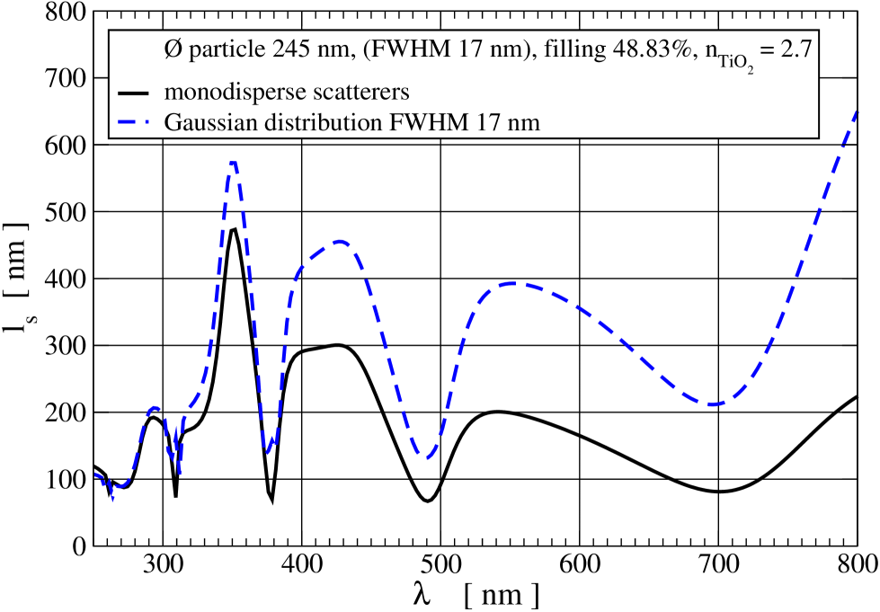
Figure 3: Scattering mean free path $l_{s}\,=\,\frac{1}{2{\rm Im}[{\sqrt{q^{2}+i{\rm Im}\Sigma(\omega)}}]}$ for two disordered samples of TiO₂ Mie spheres, the passive refractive index is $n\,=\,2.7$, the scatterers’ background is air, $\epsilon_{b}\,=\,1$. The blue dashed line shows the result for $l_{s}$ for a Gaussian distribution of scatterer sizes centered in the diameter $2\,r_{scat}\,=\,245.0\,nm$, full width half maximum is $17.0\,nm$, see Fig. (1). The filling fraction is $48.83\%$. The black line shows the result for $l_{s}$ for monodisperse Mie scatterers of the diameter of $2\,r_{scat}\,=\,245.0\,nm$, all other parameters are the same. We find that the scattering mean free path $l_{s}$ for the Gaussian distribution of scatterers is overall increased compared to the monodisperse scatterers, the quality of the results persists, however the very pronounced Mie resonances, the sharp dips of $l_{s}$, for $\lambda\,=\,310.0\,nm$ and $\lambda\,=\,380.0\,nm$ are reduced.

In Fig. (3) we show the scattering mean free path $l_{s}$ for a Gaussion distribution of Mie scatterers, see Fig. (1), which is centered at the radius of $r_{scat}\,=\,122.5\,nm$, the full width half maximum is $17.0\,nm$, and we compare it to results for monodisperse Mie scatterers of size $r_{scat}\,=\,122.5\,nm$. The description takes advantage of the fact that scattering matrices of independent scatterers are additive in general. We find that the principal Mie characteristics of the central particle size $r_{scat}\,=\,122.5\,nm$ is qualitatively conserved but quantitatively reduced. This is intuitively clear due to the additivity of scattering matrices in the independent scatterers approach since no additional structural effects, e.g. in the sense of a varying concentration of surface defects or the occurrence of correlated clusters and glass transitions, are considered so far to induce any additional dependencies. The exact Mie resonance positions, the minima of $l_{s}$, remain spectrally fixed for the Gaussian distribution of polydisperse scatterers ensembles compared to the monodisperse ensembles. What can be definitely deduced is that the scattering mean free path $l_{s}$ overall is prolonged for the Gaussian distribution which means that the scattering strength of the disordered sample is effectively reduced for polydisperse media. For wavelengths $\lambda\,=\,490.0\,nm$, $\lambda\,=\,540.0\,nm$, and $\lambda\,=\,700.0\,nm$ a reduction of the factor of 2 and more in the magnitude of the scattering mean free path $l_{s}$ is derived. The filling fraction for the result of Fig. (3) is kept constant at $48.83\,\%$. The scattering strength and thus also the probability to reach the regime of strong localization of light are significantly reduced for narrow peaked polydisperse scatterers distributions compared to monodisperse ensembles.

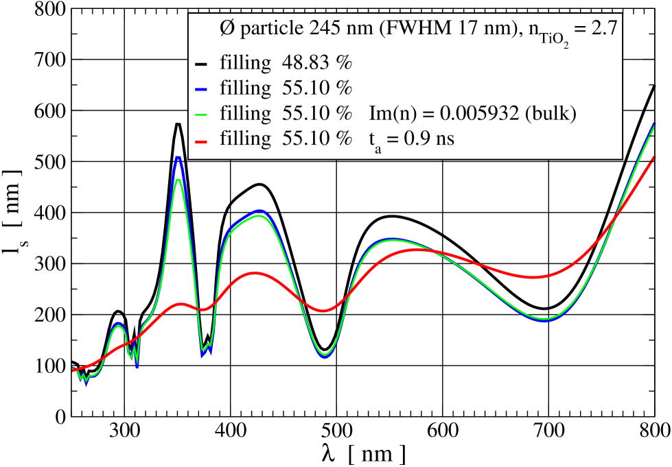
Figure 4: Scattering mean free path $l_{s}$ for disordered samples of TiO₂ Mie spheres, $n\,=\,2.7$, with a Gaussian distribution of scatterers peaked at $2\,r_{scat}\,=\,245.0\,nm$, full width half maximum is $17.0\,nm$, see Fig. (1). The scatterers’ background is air, $\epsilon_{b}\,=\,1$. We display results for the filling fractions of $48.83\,\%$ and $55.10\,\%$ of passive scatterers and we show for the filling fraction of $55.10\%$ results for active scatterers. The green line is the result for the literature value of absorption ${\rm Im}(n)\,=\,0.005932$ for bulk, the red line is a result for $\tau_{a}\,=\,0.9\,ns$ which is equivalent to ${\rm Im}(n)=0.3$. We find with an increasing filling fraction an overall decrease of $l_{s}$ while its qualitative behavior is conserved. We find that the increase of $\tau_{a}$, so the increase of loss, that the Mie resonances wash out. However it is already visible, that all results for one specific filling fraction cross in what can be mathematically identified as the inflection points. This behavior is confirmed by the behavior of the diffusion coefficient $D$, see Fig.5.

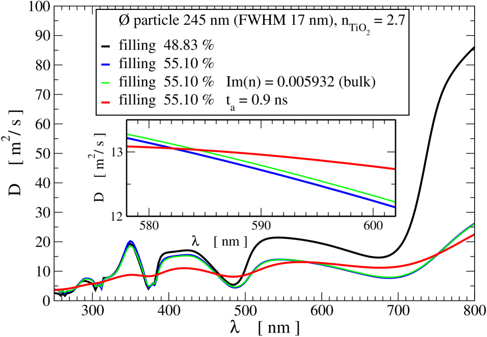
Figure 5: Real part of the diffusion coefficient $ReD$, see Eq. (33), for samples of disordered TiO₂ samples, parameters are equal to Fig.4. We find that the increase of the filling fraction rather moderately effects the quantitative behavior of ${\rm Re}D$ in the spectral region below $\lambda<490.0\,nm$, so $\lambda\,<\,4\cdot r_{scat}$, for $\lambda>490.0\,nm$ we find, that the influence of the filling increases. We find that the effect of the bulk value for absorption of ${\rm Im}(n)\,=\,0.005932$ on the diffusion coefficient for moderate excitation is peaked at $\lambda\,=\,350.0\,nm$ (green line), while it is almost undetectable in other spectral positions. The increase of absorption to $\tau_{a}\,=\,0.9\,ns$ results in the same crossing point as found for $l_{s}$ at the inflection points. Its physical meaning is rather important. Absorption or gain will rather hardly be measured at the inflection points. In the inset we show the crossing at $\lambda\,=\,583.0\,nm$ which has been confirmed in Maret2012 ; NPHOT2013 experimentally. It is found that a value of absorption, as it is commonly detected in experiments with TiO₂ powders Maret2012 ; NPHOT2013 can eliminate almost completely the size dependent influences of the scatterers geometry in the diffusion characteristics of random ensembles.

In Fig. (4) we show the results for the scattering mean free path $l_{s}$ for the Gaussian distribution of scatterers of the filling fractions $48.83\,\%$ and $55.10\,\%$ for passive Mie resonators as well as for absorbing scatterers. For the absorption we consider the literature value for TiO₂ bulk of ${\rm Im}(n)\,=\,0.005932$ as well as experimentally relevant absorption values for disordered granular arrangements. We find that the material characteristics of the scattering mean free path $l_{s}$ for an increase of the filling fraction from $48.83\,\%$ to $55.10\,\%$ is quantitatively reduced, whereas is is qualitatively confirmed. No crossover between both results is found all over the spectrum. For moderate absorption of a literature value for bulk titania, ${\rm Im}(n)\,=\,0.005932$, the magnitude of $l_{s}$ generally persists, however it is already visible for $\lambda\,=\,260.0\,nm$ to $\lambda\,=\,270.0\,nm$, $\lambda\,=\,305.0\,nm$ to $\lambda\,=\,320.0\,nm$, $\lambda\,=\,370.0\,nm$ to $\lambda\,=\,385.0\,nm$, and for $\lambda\,=\,485.0\,nm$ to $\lambda\,=\,495.0\,nm$ that the Mie resonances are washed out and $l_{s}$ is increasing. The peak positions of the characteristics at $\lambda\,=\,345.0\,nm$ to $\lambda\,=\,360.0\,nm$, $\lambda\,=\,430.0\,nm$ to $\lambda\,=\,445.0\,nm$ show a decrease of $l_{s}$ for moderate absorption. By increasing the absorption up to the value of ${\rm Im}(n)\,=\,0.3$ which is corresponding to $\tau_{a}\,=\,0.9\,ns$ we find that the Mie resonances are further reduced. For the filling fraction of $55.10\,\%$ there is a crossover of all results of $l_{s}$ found. It can be deduced that for one specific distribution of Mie scatterers sizes and varying loss parameters and identical parameters otherwise spectral points or at least narrow spectral regions exist where the loss is barely detectable by the coherent backscattering or the coherent forward scattering experiment. This loss-insensitive point is located approximately at the turning points of the results for $l_{s}$. In the dips and the peaks of $l_{s}$ loss and gain is most efficiently detected. Speaking in terms of the scattering strength of the disordered sample, it is interesting, that while absorption reduces the resonators influence in general and thus leads to the reduction of the scattering strength in the Mie resonance position, it leads to a remarkable increase of the scattering strength of the ensemble in all off-resonant cases, e.g. for $\lambda\,=\,270.0\,nm$ to $\lambda\,=\,300.0\,nm$, $\lambda\,=\,320.0\,nm$ to $\lambda\,=\,367.0\,nm$, $\lambda\,=\,390.0\,nm$ to $\lambda\,=\,470.0\,nm$, and for $\lambda\,=\,515.0\,nm$ to $\lambda\,=\,580.0\,nm$. This effect is pronounced for monodisperse samples.

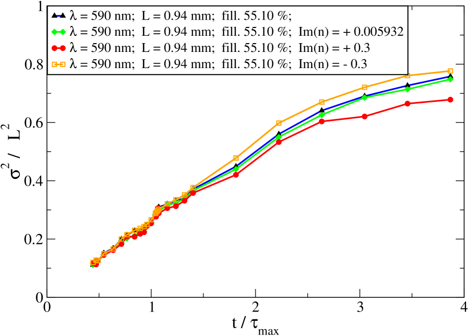
Figure 6: Temporal evolution of $\sigma^{2}(t)/L^{2}$, the cross section of the transmitted photon density (1/e). The samples extent is $L\,=\,0.94\,mm$, $n\,=\,2.7$, the samples filling is $55.10\%$. The Gaussian distribution of scatterers is centered at the diameter of $2\,r_{scat}\,=\,245.0\,nm$, full width half maximum is $17.0\,nm$. The scatterers’ background is air, $\epsilon_{b}\,=\,1$. The analysing pulse is characterized by it’s center, which is $\lambda\,=\,590.0\,nm$, full width half maximum is $250.0\,fs$, beam waist on the glass surface at focus is $100.0\,\mu m$, the pulse transition time is $\tau_{max}\,=\,2.42\,ns$, see Fig.(1). The result is normalized to the peak transition time. We display the passive complex system (black), the same arrangement including the literature value for absorption of TiO₂ bulk, ${\rm Im}\,(n)\,=\,0.005932$ (green), an experimentally relevant value for absorption of disordered random TiO₂ media ${\rm Im}\,(n)\,=\,+0.3$ (red), and the same scatterers arrangement with refractive index $n\,=\,2.7$ as it is pumped and gain assumes a value of ${\rm Im}\,(n)\,=\,-0.3$ (yellow). For all parameters a plateau in the temporal evolution of $\sigma^{2}(t)/L^{2}$ is found as a characteristics of the complex medium in the long time limit. Whereas for gain the spreading of the cross-section overall is increased, absorption generally seems to lead to an earlier inset of the plateau effect. Results for the passive system (black), ${\rm Im}\,(n)\,=\,0.005932$ (green) and ${\rm Im}\,(n)\,=\,+0.3$ (red) are to be compared to results of the scattering mean free path $l_{s}$ Fig. (3), and to the diffusion coefficient $D$, Fig. (5), at $\lambda\,=\,590.0\,nm$.

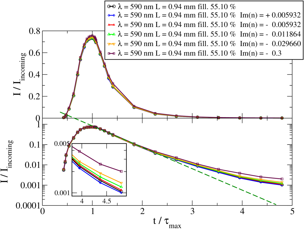
Figure 7: Temporal evolution of intensity transmission $I/I_{incoming}$. $I$ is the time-dependent, surface- and angle-integrated count rate at the detector. $I_{incoming}$ is the time-, surface- and angle-integrated count rate at the detector. The green line marks the behavior of purely diffusive transport, the deviation to coherent transport, see black line and circles, in the log-plot is significant. The result is normalized to the peak transition time $\tau_{max}\,=\,2.42\,ns$. The bottom panel shows the log-plot of the result where the green dashed line marks the diffusive limit. We display results for the passive case (black), and the same arrangement including the literature value for absorption of TiO₂ bulk, ${\rm Im}\,(n)\,=\,0.005932$, (blue). One finds that absorption is pulling the result in the long time limit towards the purely diffusive case. Gain on the other hand, ${\rm Im}\,(n)\,=\,-0.005932$, ${\rm Im}\,(n)\,=\,-0.005932$ (red), ${\rm Im}\,(n)\,=\,-0.011864$ (green), ${\rm Im}\,(n)\,=\,-0.029660$ (orange), and ${\rm Im}\,(n)\,=\,-0.3$ (maroon), yields a lift of the result in the long time limit.

The diffusion coefficient $D$ as it is formally derived in Eq. (33) can in principal be a complex quantity where the imaginary part ${\rm Im}D$ becomes of physical relevance for pumped active complex matter near or at the laser threshold. In coherent backscattering experiments and in coherent forwardscattering experiments the real part of the diffusion coefficient $ReD$ plays the crucial role Fig. (5). $ReD$ is commonly addressed in the literature as the diffusion constant $D$ and it can be implicitly measured. For an absorbing polydisperse sample, $\tau_{a}\,=\,0.9\,ns$ and ${\rm Im}(n)\,=\,0.3$, we find that almost any Mie characteristics is washed out due to the absorptive character of the single scatterer. A destructive interplay between absorption characteristics and the resonator properties is developed all over the electromagnetic excitation spectrum. Extremely pronounced is the difference in the magnitude of the diffusion coefficient $D$ for wavelengths larger than $\lambda\,=\,700.0\,nm$. When the filling is enhanced from $48.83\,\%$ to $55.10\,\%$ the diffusion coefficient $D$ at $\lambda\,=\,800.0\,nm$ is reduced from $85\,m^{2}/s$ to $25\,m^{2}/s$ so approximately to $30\,\%$. Is shall be pointed out here that there is no transition to an ordered sample considered and all results are derived for homogeneous disordered but polydisperse samples of the mentioned Gaussian distribution of scatterer radii. We display one of the crossover points in the inset of Fig. (5) the diffusion coefficient $D$ which is in the vicinity of the wavelength $\lambda\,=\,583.0\,nm$.

When we discuss these results for $l_{s}$ and $D$, in terms of the Ioffe-Regel criterium with the benchmark of strong localization of light, we find $kl\,<\,1$ could be experimentally derived for the monodisperse case, see Fig. (3), e.g. in the Mie resonance at $\lambda\,=\,490.0\,nm$, whereas for the polydisperse ensemble $kl\,=\,1.67$ the condition is not strictly fulfilled and interference effects will play a subtle role. It can thus be concluded that the probability to find Anderson localized photons will be enhanced in the monodisperse ensemble where a factor of 2 enhancement with respect to the incoming intensity could be detected. The increase of the volume filling fraction for polydisperse samples will only have a moderate impact in the search for Anderson localized photons, whereas absorption, which is enhanced in disordered granular media as compared to the bulk case, is a crucial and limiting factor, see Fig. (4). Thus it is important to find a systematic theoretical method to distinguish micro- and macroscopic structural effects in the signal which is a mix of both.

III.2 Temporal evolution of the transmission cross section and the transmitted intensity

In section Quantum Field Theory for Multiple Scattering of Photons II we presented the theory to study the propagation and the localization of a laser pulse through a disordered ensemble of complex scatterers. The solution of this framework in the sense of the simulation of detectable scattered intensity is not restricted to a dimension or a direction. Transmission optical coherence tomography based measurements of optical material properties is one experimental platform for our methodology Hee ; Zaccanti ; Trull . Here we present results for the temporal evolution of the transmission cross section $\sigma$, and the mean square width $\sigma^{2}$ respectively, Fig. (6), and the temporal dependency of the transmitted photonic intensity, Fig. (7). Our results are derived for homogeneous disordered samples with a Gaussian distribution of scatterer diameters centered at $d\,=\,245.0\,nm$ and $55.10\,\%$ volume filling. This is the strongly scattering and strongly disordered regime. We display results for the excitation laser frequency of $\lambda\,=\,590.0\,nm$, where we know $kl_{s}\,=\,3.62$ from previous results, see Fig. (4). In terms of the Ioffe-Regel criterium this case should be far off any case of the Anderson localization regime, thus the aim of our considerations is to determine the number of coherently interfering photons as the deviation from the purely diffusive case. The mean square width Buehrer ; Maret2012 ; NPHOT2013

$$\sigma^{2}(t)\,=\,\frac{\int r^{2}P_{E}(r,t)\,d^{2}r}{\int P_{E}(r,t)\,d^{2}r}$$ (51)

is defined as the square of the up to the full-width-half-maximum (FWHM) limit integrated area $\sigma$ of the transmitted transverse intensity distribution at the ensemble surface, see Fig.(1). We display this characteristics in Fig. (6) normalized to the square of the samples length $L^{2}$.

We find that the transmission cross section, the mean square width, Fig. (6), is definitely depending on absorption and gain of the complex random medium, and it is a very sensitive measure. In Fig. (6) we display results for the temporal evolution of $\sigma^{2}/L^{2}$ for the wavelength of the incident pulse of $\lambda\,=\,590.0\,nm$. The case of $\lambda\,=\,590.0\,nm$ is extremely close to the crossing point or turning point of the scattering mean free path $l_{s}$, Fig. (4), and the corresponding diffusion coefficient $D$, Fig. (5). While the characteristics $l_{s}$ and $D$ are almost insensitive to absorption at $\lambda\,=\,590.0\,nm$, a clear deviation of $\sigma^{2}/L^{2}$ for the case of ${\rm Im}(n)\,=\,+0.3$ from the passive case of about $12\,\%$ is found in the temporal limit of $t/\tau_{max}\,=\,4$. In Fig. (7) we show the results for the transmitted intensity $I/I_{incident}$ in the long time limit. The purely diffusive case is marked in the log-plot as the dashed green line. It can be concluded for the strictly passive case (black line) that the increase of the transmission in the long-time limit in comparison to the diffusive case with the exponential decay is the number of localized photons, that have been multiply and coherently scattering and interfering in the disordered medium in the sense of the maximally crossed processes, represented diagrammatically by the Cooperon, see Fig. (1). It is further derived that absorption, incorporated by the literature value for bulk TiO₂, ${\rm Im}(n)\,=\,+0.005932$ (blue line), reduces the number of localized photons, and the long time behavior of $P_{E}$ retrogrades towards the diffusive limit. This result as such has been expected. By comparison of the relative magnitude of the results for $\sigma^{2}/L^{2}$ with the transmitted intensity $P_{E}$, Fig. (7), it is however interesting to note, that the plateau effect for the case of absorption is enhanced, precisely it shows an earlier onset. Thus the plateau as such seems not to be a signature of localization, however the magnitude of the deviation of the transmitted intensity $P_{E}$ from the diffusive limit can be interpreted as a sign of enhanced coherent multiple scattering and thus as an enhancement of interference effects in principle. The influence of the single Mie scatterer is noteworthy when we discuss the influence of gain. Gain as the negative imaginary part of the complex refractive index and as a negative part of the complex permittivity is a microscopic material characteristics equivalent to absorption. Whereas absorption however is a microscopic interaction where the life-times of light-matter bound states in first instance do not play a crucial role, this is different for the case of gain. Gain is achieved by an enhanced life-time of light matter bound states leading to an increase of the photon number in the incident wavelength. Gain and absorption are as such in our theory properties of the single complex Mie scatterer, and the microscopic materials characteristics is interacting with the resonator. In the case of strong external laser pulses the local density of states and thus the refractive index of TiO₂ bulk can be shifted and this effect will lead to a shift of the overall characteristics of the disordered granular medium $l_{s}$, Fig. (4), and $D$, Fig. (5). When non-linear effects, e.g. higher-order harmonics of the incident wavelength $\omega$, play a role, this processes might contribute to an enhancement of multiple scattering and of interference effects. These enhancements can result in time of flight experiments is a variety of observations, such as off-centered peak in the integrated spectrum. In this article we discuss gain in the central wavelength of the incident pulse, which can originate from light-matter bound states of higher harmonics, so non-linear effects play a role even though the system is far below any laser threshold. The gain is visible on the one hand side as a delayed onset of the plateau of $\sigma^{2}/L^{2}$ on the one hand, see Fig. (6) (yellow line), on the other hand we find an increase in the transmitted coherent photon intensity in the long-time limit, Fig. (7). The variation of $P_{E}$ due to enhanced multiple scattering and interference effects due to an increased filling of due to enhanced resonator properties of the geometrical scatterer can thus be well determined and distinguished by comparing the characteristics of $l_{S}$, $D$, $\sigma^{2}/L^{2}$ and $P_{E}$ from effects incorporating gain and absorption.

IV Conclusions

We have presented in this article an innovative method for characterizing disordered complex random media based on a quantum-field theoretical approach, the Vollhardt-Wölfle theory, for photonic transport including interference effects in multiple scattering processes. Our theory incorporates the Ward-Takahashi identity for photonic transport and thus enables us to determine self-consistent results for the material characteristics of disordered granular complex media. We solve the theory in three dimensions space- and time-dependent with a weighted essentially non-oscillatory solver method (WENO). The solution with the WENO solver enables us to determine results for ultrashort analyzing pulses and pump-probe experiments, since we can deal with highly non-linear processes and discontinuities. We have presented here a systematic study of the scattering mean free path $l_{s}$ and the diffusion coefficient $D$. These characteristics can be compared directly to experimental results derived in a coherent backscattering experiment. They show that the resonator characteristics, e.g. the Mie resonance, plays a crucial role which is even more important, when non-linear effects, gain and absorption, are minimized by the choice of the scattering matter. It has also been shown that a polydispersity of the scatterers reduces the probability to reach an Anderson transition with transport of light. The incorporation of gain and absorption reveals, that all materials characteristics are very sensitive to such properties of complex matter. It has been shown that so called absorption-free measurements are bound to spectrally narrow areas where the resonator characteristics of the single scatterer leads to a minimized sensitivity with respect to a change of the complex refractive index and the complex permittivity. Our results for ab initio simulations of time of flight experiments yield the characteristics of the normalized transmission or reflection cross section and the absolute as well as the normalized number of coherently scattered photons. We presented results random mono- and polydisperse ensembles of TiO₂ Mie scatterers in a transmission optical coherence tomography setup. It has been demonstrated that these characteristics offer an increased sensitivity to any microscopic and the macroscopic structural modification compared to the coherent backscattering experiment. The underlying theory paves a way towards the detection of subtle interference effects due to multiple scattering events in OCT setups that may lead to an increase of the sensitivity of OCT of orders of magnitude, and furthermore it may improve the analysis of other methods of advanced spectroscopy like DWS, DLS and QFS. This effect can be enhanced by the scatterers resonances. We conclude that our combinatory analysis of underlying transport theory and its results, the scattering mean free path, the diffusion constant, and the derived characteristics in the temporal evolution is suitable to distinguish between perfectly coherent multiple scattering and interferences and on the other hand between influences of the complex random medium in the full spectrum of the analysis. We provide a consistent method, which is able to characterize disordered media in the weakly and the strongly scattering regime, the approach is suitable to incorporate ultrashort and intense light pulses and the resulting subtle local and non-local light-matter interactions on a broad temporal range. The method is ab initio not limited to light, it can be performed with the full spectrum of electromagnetic excitations and it can be transferred to any other type of wave propagation as matter waves and sound. It will be subject of subsequent work to investigate further influences of multiple scattering and higher-order non-linear effects in ensembles of clusters and composite scatterers such as shells, as well as of macromolecules that can be random or quasi-ordered and may form so called meta glasses.

Authors contributions: All authors were equally involved in the preparation of the manuscript. All the authors have read and approved the final manuscript.

Acknowledgment: The authors thank S. Fishman, L. Sanchez-Palencia, B. A. van Tiggelen, R. v. Baltz, W. Bührer, G. Maret, K. Busch and J. Kroha for highly valuable discussions.

References

- (1) E. Akkermans, P. E. Wolf, R. Maynard, Phys. Rev. Lett. 56 14, 1471-1474 (1986).
- (2) R. Pecola, J. Chem. Phys. 40, 1604 (1964).
- (3) J. W. Goodman, JOSA 66, 11, 1145-1150 (1976).
- (4) S. W. Provencher, Makromol. Chem. 180, 201-209 (1979).
- (5) C. Urban, P. Schurtenberger, J. Colloid. Interface Sci. 207 (1), 150-158 (1998).
- (6) I. Block, F. Scheffold, Rev. Sci. Instruments. 81, 12, 123107-123107-7 (2010).
- (7) C. Baravian, F. Caton, J. Dillet, J. Mougel, Phys. Rev. E 71, 066603 (2005).
- (8) D. J. Pine, D. A. Weitz, P. M. Chaikin, E. Herbolzheimer, Phys. Rev. Lett. 60 12 1134-1137 (1988).
- (9) D. Huang, E. A. Swanson, C. P. Lin, J. S. Schuman, W. G. Stinson, W. Chang, M. R. Hee, T. Flotte, K. Gregory, C. A. Puliafito, J. G. Fujimoto, Science 254 (5035) 1178-1181 (1991).
- (10) A. F. Fercher, W. Drexler, C. K. Hitzenberger, T. Lasser, Rep. Prog. Phys. 66, 239-303 (2003).
- (11) J. M. Schmitt, IEEE Journal of Selected Topics in Quantum Electronics, 5, No. 4, 1205-1214 (1999).
- (12) A. Zhang, Q. Zhang, Ch.-L. Chen, R. K. Wang, Journal of Biomedical Optics 20(10), 100901 (2015).
- (13) K. C. Zhou, R. Qian, S. Degan, S. Farsiu, J. A. Izatt, Nature Phot. doi:10.1038/s41566-019-0508-1 (2019).
- (14) A. Podoleanu, I. Charalambous, L. Plesea, A. Dogariu, R. Rosen, Phys. Med. Biol. 49, 1277 (2004).
- (15) S. John, Phys. Rev. Lett. 58, 23, 2486-2489 (1987).
- (16) F. C. MacKintosh, S. John, Phys. Rev. B 37, 4, 1884-1897 (1988).
- (17) J. F. de Boer, T. E. Milner, J. S. Nelson, Opt. Lett. 24, 300-302 (1999).
- (18) M. Yamanari, S. Tsuda, T. Kokubun, Y. Shiga, K. Omodaka, N. Aizawa, Y. Yokoyama, N. Himori, S. Kunimatsu-Sanuki, K. Maruyama, H. Kunikata, T. Nakazawa, Biomed. Opt. Express 7, 3551-3573 (2016).
- (19) N. Gosh, M. F. G. Wood, A. Vitkin, J. Biomed. Opt. 13, 044036 (2008).
- (20) B. Gompf, M. Gill, M. Dressel, A. Berrier, JOSA 35 (2) 301-308 (2018).
- (21) H. Roychowdhury, S. A. Ponomarenko, E. Wolf, J. Mod. Opt. 52(11), 1611-1618 (2005).
- (22) S.A. Ponomarenko, Opt. Lett. 40(4), 566-568 (2015).
- (23) O. Korotkova, M. Salem, A. Dogariu, E. Wolf, Waves in Random Complex Media 15(3), 353-364 (2005).
- (24) I. Voloshenko, B. Gompf, A. Berrier, M. Dressel, G. Schnoering, M. Rommel, J. Weis, Appl. Phys. Lett. 115, 063106 doi:10.1063/1.5094409 (2019).
- (25) I. M. Vellekop, C. M. Aegerter, Optics Letters 35 8, 1245 (2010).
- (26) A. P. Mosk, A. Lagendijk, G. Lerosey, M. Fink, Nature Photonics 6, 283-292 (2012).
- (27) N. Lippok, M. Siddiqui, B. J. Vakoc, B. E. Bouma, Phys. Rev. Applied 11, 014018 (2019).
- (28) M.B. Isichenko, Rev. Mod. Phys., 64, 4, 961 (1992).
- (29) Z. Y. Ou, L. J. Wang, X. Y. Zou, L. Mandel, Phys. Rev. A 41, 1597 (1990).
- (30) M. V. Chekhova, Z. Y. Ou, Adv. Opt. Photon. 8, 104 (2016).
- (31) A. F. Abouraddy, M. B. Nasr, B. E. A. Saleh, A. V. Sergienko, M. C. Teich, Phys. Rev. A 65, 053817 (2002).
- (32) M. B. Nasr, B. E. A. Saleh, A. V. Sergienko, M. C. Teich, Optics Express 12 (7), 1353-1362 (2004).
- (33) M. B. Nasr, B. E. A. Saleh, A. V. Sergienko, M. C. Teich, Phys. Rev. Lett. 91, 083601 (2003).
- (34) A. Amon, A. Mikhailovskaya, J. Crassous, Review of Scientific Instruments 88, 051804 (2017).
- (35) S. Fuchs, C. Rödel, A. Blinne, U. Zastrau, M. Wünsche, V. Hilbert, L. Glaser, J. Viefhaus, E. Frumker, P. Corkum, E. Förster, and G. G. Paulus, Sci. Rep. 6, 20658 (2016).
- (36) A. Valles, G. Jimenez, L. J. Salazar-Serrano, J. P. Torres, Phys. Rev A 97, 023824 (2018).
- (37) D.V. Novitsky, EPL, 99 44001 (2012).
- (38) G. J. Tearney, M. E. Brezinski, J. F. Southern, B. E. Bouma, M. R. Hee, and J. G. Fujimoto, Opt. Lett. 20, 2258-2260 (1995).
- (39) A. Knuttel, M. Boehlau-Godau, J. Biomed. Opt. 5, 83-92 (2000).
- (40) A. V. Zvyagin, K. K. M. B. D. Silva, S. A. Alexandrov, T. R. Hillman, J. J. Armstrong, T. Tsuzuki, D.D. Sampson, Opt. Express 11, 3503-3517 (2003).
- (41) B. B. Das, F. Liu, R. R. Alfano, Rep. Prog. Phys. 60, 227-292 (1997).
- (42) M. C. W. van Rossum, Th. M. Nieuwenhuizen, Rev. Mod. Phys. 71, 313 (1999).
- (43) R. Savo, R. Pierrat, U. Najar, R. Carminati, S. Rotter, S. Gigan, Science, 358 (6364), 765-768 (2017).
- (44) S. Rotter, S. Gigan, Rev. Mod. Phys. 89, 015005 (2017).
- (45) K. Vishwanath, B. Pogue, M.-A. Mycek, Phys. Med. Biol. 47, 3387-3405 (2002).
- (46) B. Redding, A. Cerjan, X. Huang, M. Larry Lee, A. D. Stone, M. A. Choma, H. Cao, PNAS 112 (5) 1304-1309 (2015).
- (47) O. Liba, M. D. Lew, E. D. SoRelle, R. Dutta, D. Sen, D. M. Moshfeghi, S. Chu, A. de la Zerda, Nat. Comm. 8:15845 (2017).
- (48) T.-M. Sun, C.-S. Wang, C.-S. Liao, S.-Y. Lin, P. Perumal, C.-W. Chiang, Y.-F. Chen, ACS Nano 9(12), 12436-12441 (2015).
- (49) K. V. Chellappan, E. Erden, H. Urey, Appl. Opt. 49, F79-F98 (2010).
- (50) A. Badon, D. Li, G. Lerosey, A. C. Boccara, M. Fink, A. Aubry, Sci. Adv. 2016; 2 : e1600370 (2016).
- (51) G. Jacucci, J. Bertolotti, S. Vignolini, Adv. Optical Mater. 1900980 (2019).
- (52) P.D. Garcia, R. Sapienza, A. Blanco, C. Lopez, Adv. Mater. 19:2597-2602 (2007).
- (53) N. Senbil, M. Gruber, C. Zhang, M. Fuchs, F. Scheffold, Phys. Rev. Lett. 122, 108002 (2019).
- (54) R. Frank, A. Lubatsch, J. Kroha, Phys. Rev. B 73, 245107 (2006).
- (55) R. Frank, A. Lubatsch, Phys. Rev. A 84, 013814 (2011).
- (56) Chi-Wang Shu, NASA/CR-97-206253. ICASE Report 97-65, (1997).
- (57) A. Harten, B. Engquist, S. Osher, S. R. Chakravarthy, Journal of Computational Physics 71, 231-303 (1987).
- (58) C.-W. Shu, S. Osher, Journal of Computational Physics 77, 439-471 (1988).
- (59) X. Liu, S. Osher, T. Chan, Journal of Computational Physics 115, 200-212 (1994).
- (60) Y.-T. Zhang, J. Shi, C.-W. Shu, Y. Zhou, Phys. Rev E 68, 046709 (2003).
- (61) P. D. Lax, R. D. Richtmyer, Comm. Pure Appl. Math. 9, 267-293 (1956).
- (62) J. S. Hesthaven, T. Warburton, Philosophical Transactions of the Royal Society A: Mathematical, Physical and Engineering Sciences, 362 (1816), 493-524 (2004).
- (63) D. Vollhardt, P. Wölfle, Phys. Rev. Lett. 45, 842 (1980);
- (64) D. Vollhardt, P. Wölfle, Phys. Rev. B 22, 4666 (1980).
- (65) P. W. Anderson, Phys. Rev. 109, 1492 (1958).
- (66) A. A. Chabanov, M. Stoytchev, A. Z. Genack, Nature 404, 850–853 (2000).
- (67) A. Lagendijk, B. v. Tiggelen, D. S. Wiersma, Physics Today 62 (8), 24 (2009).
- (68) T. Schwartz, G. Bartal, S. Fishman, M. Segev, Nature 446, 52-55 (2007).
- (69) J. W. Fleischer, M. Segev, N. K. Efremidis, D. N. Christodoulides, Nature 422, 147-150 (2003).
- (70) N. Garcia, A. Z. Genack, Phys. Rev. Lett. 66 1850-1853 (1991).
- (71) P. Henseler, J. Kroha, B. Shapiro Phys. Rev. B 78, 235116 (2008).
- (72) C. A. Müller, D. Delande, B. Shapiro, Phys. Rev. A 94, 033615 (2016).
- (73) J. Billy, V. Josse, Z. Zuo, A. Bernard, B. Hambrecht, P. Lugan, D. Clement, L. Sanchez-Palencia, O. Bouyer, A. Aspect, Nature 453 (7197), 891-894 (2008).
- (74) H. Hu, A. Strybulevych, J.H. Page, S.E. Skipetrov, B.A. van Tiggelen, Nat. Phys. 4, 945 (2008).
- (75) T. Sperling, W. Bührer, C. M. Aegerter, G. Maret, Nature Photon. 7, 48-52 (2013).
- (76) F. Scheffold, D. Wiersma, Nature Photon. 7 (12), 934 doi: 10.1038/nphoton.2013.210 (2013).
- (77) G. Maret, T. Sperling, W. Bührer, A. Lubatsch, R. Frank, C.M. Aegerter, Nature Photon. 7 (12), 934-935 doi:10.1038/nphoton.2013.281 (2013).
- (78) J. Richard, L.-K. Lim, V. Denechaud, V. V. Volchkov, B. Lecoutre, M. Mukhtar, F. Jendrzejewski, A. Aspect, A. Signoles, L. Sanchez-Palencia, V. Josse, Phys. Rev. Lett. 122, 100403 (2019).
- (79) Z. V. Vardeny, A. Nahata, A. Agrawal, Nature Phot. 7, 177-187 (2013).
- (80) J.I. Gersten, D.A. Weitz, T.J. Gramila, A. Z. Genack, Phys. Rev. B 22, 10, 4562-4571 (1980).
- (81) J. C. J. Paasschens, T. Sh. Misirpashaev, C. W. J. Beenakker, Phys. Rev. B 54, 11887 (1996).
- (82) C. C. Evans, J. D. B. Bradley, E. A. Marti-Panameno, E. Mazur, Optics Express 20, 3, 3118 (2012).
- (83) G. Chakravarthy, S. R. Allam, A. Sharan, J. Nonlinear Optic. Phys. Mat. 25, 2, 1650019 (2016).
- (84) L. Sanchez-Palencia, M. Lewenstein, Nat. Phys. 6, 81 (2010).
- (85) G. Mie, Ann. Phys. (Leipzig) 330, 377 (1908).
- (86) A. Lubatsch, J. Kroha, K. Busch, Phys. Rev. B 71, 184201 (2005).
- (87) M. Wegener, Extreme Nonliner Optics, ISBN 3-540-22291-X, Springer (2004).
- (88) G.F. Bohren, D.R. Huffman, Absorption and scattering of light by small particles. John WileySons (1983).
- (89) M. Störzer, C. M. Aegerter, G. Maret, Phys. Rev. Lett. 96, 063904 (2006).
- (90) M. Störzer, C. M. Aegerter, G. Maret, Phys. Rev. E 73, 065602(R) (2006).
- (91) W. Bührer, Anderson Localization of Light in the Presence of Non-linear Effects, Dissertation, http://nbn-resolving.de/urn:nbn:de:bsz:352-207872 (2012).
- (92) R. Sapienza, P.D. Garcia, J. Bertolotti, M. D. Martin, A. Blanco, L. Vina, C. Lopez, D.S. Wiersma, Phys. Rev. Lett. 99 233902 (2007).
- (93) P. D. Garcia, R. Sapienza, J. Bertolotti, M. D. Martin, A. Blanco, A. Altube, L. Vina, D. S. Wiersma, C. Lopez, Phys. Rev. A 78, 023823 (2008).
- (94) M. Burresi, V. Radhalakshmi, R. Savo, J. Bertolotti, K. Vynck, D. S. Wiersma, Phys. Rev. Lett. 108, 110604 (2012).
- (95) M. Ghulinyan, C. J. Olton, L. Dal Negro, L. Pavesi, R. Sapienza, M. Colocci, D.S. Wiersma, Phys. Rev. B 71 09204 (2005).
- (96) D.S. Wiersma, A. Lagendijk, Phys. Rev. E 54, 4256-4265 (1996).
- (97) R. Kubo, J. Phys. Soc. Japan 12, 570 (1957). See also R. Kubo, in Lectures in Theoretical Physics, W. E. Brittin and L. G. Dunham, Eds. (Interscience Publishers, Inc. , York, 1959), Vol. I, p. 120.
- (98) R. L. Peterson, Rev. Mod. Phys. 39, 1, 69-77 (1967).
- (99) A. Lubatsch, R. Frank, Eur. Phys. J. B, 92: 215 (2019).
- (100) A. Lubatsch, R. Frank, Symmetry 11, 1246 (2019).
- (101) A. Lubatsch, R. Frank, Appl. Sci. 10(5), 1836 (2020).
- (102) L. E. Reichl, M. D. Porter, Phys. Rev. E, 97 (4) 042206 (2018).
- (103) J. C. Ward, Phys. Rev. 78, 2, 182 (1950).
- (104) Y. Takahashi, Il Nuovo Cimento Vol. VI, 2, 371-375 (2231 - 2235) (1957).
- (105) J. Kroha, Physica A: Statistical Mechanics and its Applications, Vol. 167, issue 1, 231-252 (1990).
- (106) L. Onsager, Phys. Rev. 37, 405-426 (1931).
- (107) L. Onsager, Phys. Rev. 38, 2265 (1931).
- (108) K. L. van der Molen, P. Zijlstra, A. Lagendijk, A. P. Mosk, Opt. Lett. 31, 1432 (2006).
- (109) A. Lubatsch, R. Frank, New J. Phys. 16, 083043 (2014).
- (110) A. Lubatsch, R. Frank, Scientific Reports 5, 17000 (2015).
- (111) A. Lubatsch, R. Frank Appl. Sci. 9, 2477 (2019).
- (112) K. Busch, C.M. Soukoulis, Phys. Rev. Lett. 75, 3442 (1995); Phys. Rev. B 54, 893 (1996).
- (113) B. A. van Tiggelen, A. Lagendijk, M. P. van Albada, A. Tip, Phys. Rev. B 45, 12233 (1992).
- (114) B. A. van Tiggelen, A. Lagendijk, A. Tip, Phys. Rev. Lett. 71, 1284 (1993).
- (115) M. R. Hee, J. A. Izatt, J. M. Jacobson, J. G. Fujimoto, Opt. Lett. 18, (12), 950-952 (1993).
- (116) G. Zaccanti, S. D. Bianco, and F. Martelli, Applied Optics 42, (19) 4023 (2003).
- (117) A. K. Trull, J. van der Horst, J. G. Bijster, J. Kalkman, Optix Express 23, (26) 33550 (2015).