A Geometric Interpretation of the Quadratic Formula

Abstract

This article provides a simple geometric interpretation of the quadratic formula. The geometry helps to demystify the formula’s complex appearance and casts it into a much simpler existence, thus potentially benefits early algebra students.

1 Introduction

This work came from a note I wrote down several years back. Motivated by the recent coverage of Po-Shen Lo’s work [1], I decide it could worth sharing. It is my hope that this short article will add yet another pleasant aspect to the time-honored quadratic formula. To keep it short, the author will not review the rich history behind the quadratic formula, and instead highly recommend readers to consult Lo’s article [1] and references therein.

2 Derivation

The quadratic formula gives the roots to the algebraic equation $ax^{2}+bx+c=0$. Without loss of generality, we set $a=1$ and assume $b>0$ and $c>0$. So we are left with

$$x^{2}+bx+c=0$$ (1)

to solve. Let us first start with a simpler function (or curve)

$$y=x^{2}+bx.$$ (2)

Algebraically, its roots are solutions to the equation $y=x^{2}+bx=0$, which are clearly $x_{1}=0$ and $x_{2}=-b$. Geometrically, its roots are the intersection of the curve with the $x$-axis, which are marked by the two red dots in Fig. 1.

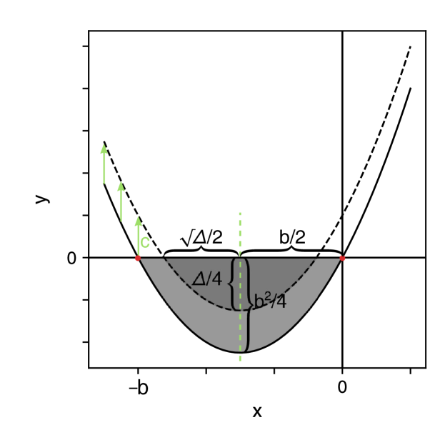
Figure 1: The curves $y=x^{2}+bx$ (solid, associated with the light-shaded region) and $y=x^{2}+bx+c$ (dashed, associated with the dark-shaded region). The green arrows indicate how the two curves are related: by a vertical shift.

Before adding $c$ back, we should realize two geometric properties of curve 2 (see Fig. 1).

1. Both the curve and its two roots are symmetric about $x=-b/2$ (the vertical dashed line in green). This property is quite intuitive from Fig. 1 and can be shown by averaging the two roots. When we add $c$ back, we merely lift the curve vertically upward. Thus, the symmetry is respected.

2. For easy reference, we refer to the region between the $x$-axis and the part of curve below it as the “valley”. They are shaded in Fig. 1. The “half-width” of this valley is $b/2$, and the “depth” of this valley is $b^{2}/4$. While the depth can be found by directly substituting $x=-b/2$ into the equation, a better way is to use the quadratic nature of the curve: as one travels along the curve from its very bottom, the vertical shift equals the square of the horizontal shift by definition. Naturally, the depth of the valley (here the vertical shift) equals the square of the half width of the valley (here the horizontal shift). Conversely, the half-width of the valley equals the square root of the valley depth.

Now we add $c$ back. By item 1, adding $c$ lifts $y=x^{2}+bx$ vertically upward by an amount of $c$, so the valley is shallower and its new depth is $\frac{b^{2}}{4}-c$. By item 2, we know that the half width of the new valley is $\sqrt{\frac{b^{2}}{4}-c}$. Because the two new roots are still symmetric about $x=-b/2$, we have the roots

$$-\frac{b}{2}\pm\sqrt{\frac{b^{2}}{4}-c},$$ (3)

or in the more familiar form:

$$\frac{-b\pm\sqrt{b^{2}-4c}}{2}.$$ (4)

3 Discussion

3.1 Alternative split

In this article, the author splits Eq. 1 into $x^{2}+bx=0$ and $+c$ to derive the geometric interpretation. He also tried other ways of splitting. For example, $x^{2}+c$ and $bx$, or $x^{2}$ and $bx+c$. They failed to work due to that the term $bx$ or $bx+c$ represents a slanted line, making it hard to proceed. It is likely that the split used by this article is the easiest one that yields to clear geometric interpretations.

3.2 The discriminant

An interesting observation is that the discriminant of the quadratic equation $\Delta=b^{2}-4c$ is nothing but the full width of the valley squared. Certainly, there will be no roots when this value is negative. Yet another interpretation is that the depth of the valley is $\frac{1}{4}\Delta=\frac{b^{2}}{4}-c$. When it is negative, the valley is non-existent, the curve is above the $x$-axis (by an amount of $-\frac{1}{4}\Delta$), and there are no roots.

At this point, it is clear that a positive $c$ always tries to eliminate the valley and roots. Whereas $b$, regardless of its sign, always creates two roots. In this sense, the two coefficients compete against each other.

3.3 Pedagogy

For the students to follow this article, it is vital that they first comprehend the geometry of quadratic curves. The part likely needs the most explanation is item 2 of the previous section, which relates the horizontal and vertical changes of the curve, as one travels along it from its very bottom.

As a final comment. Eq. 3 seems to have clearer meaning than Eq. 4. In the author’s opinion, there are clear geometric interpretations of each value and operator in Eq. 3; a heavily annotated version of which is shown in Fig. 2. Much of these interpretations are lost in Eq. 4, leaving a lifeless instruction waiting to be executed mechanically.

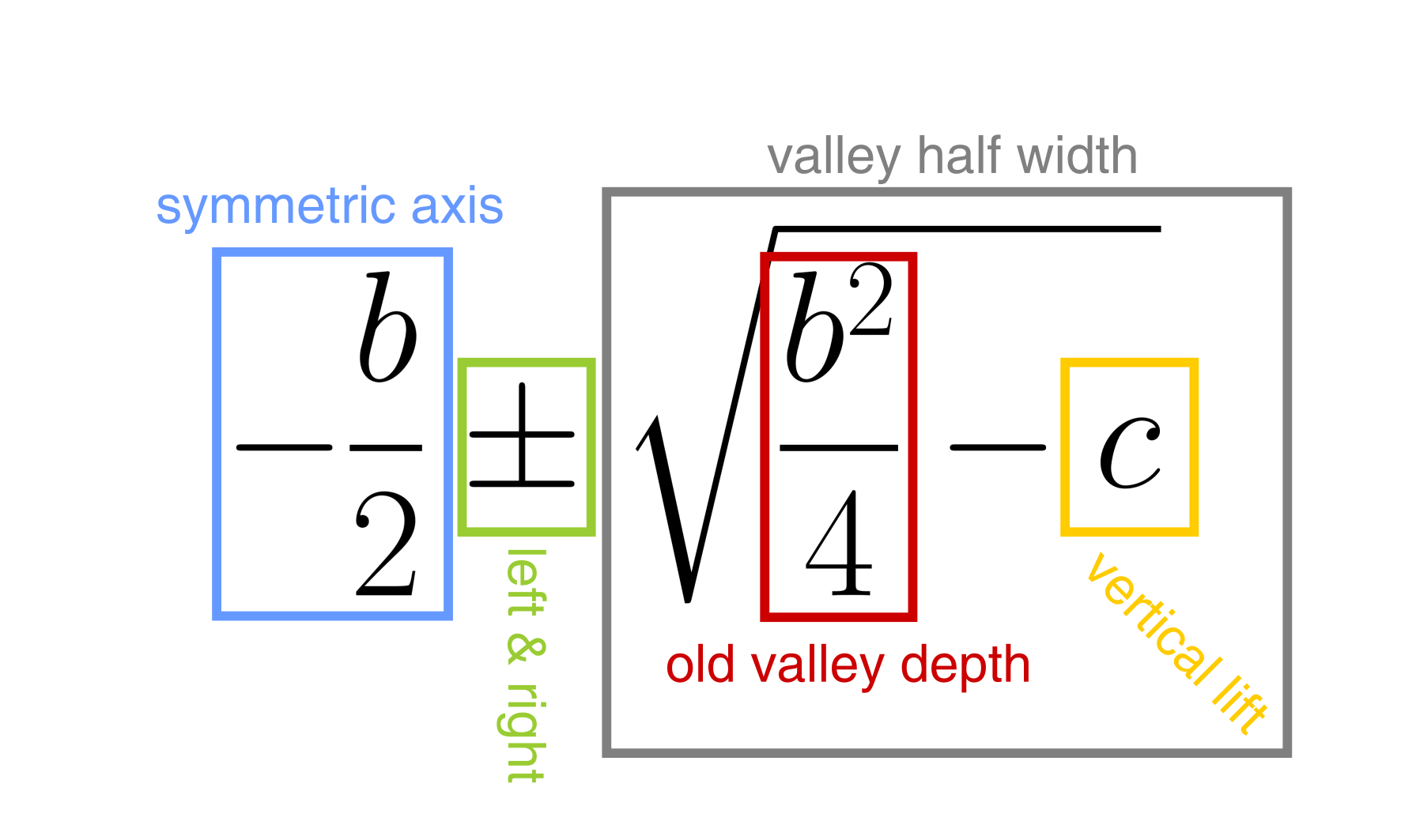
Figure 2: Eq. 3, with each term annotated by its geometric meaning .

References

- [1] Loh, Po-Shen. (2019). A Simple Proof of the Quadratic Formula. arXiv preprint arXiv:1910.06709.