A physically motivated definition for the size of galaxies in an era of ultra-deep imaging

Abstract

Present-day multi-wavelength deep imaging surveys allow to characterise the outskirts of galaxies with unprecedented precision. Taking advantage of this situation, we define a new physically motivated measurement of size for galaxies based on the expected location of the gas density threshold for star formation. Employing both theoretical and observational arguments, we use the stellar mass density contour at 1 $M_{\rm\odot}$ pc^-2 as a proxy for this density threshold for star formation. This choice makes our size definition operative. With this new size measure, the intrinsic scatter of the global stellar mass ($M_{\rm\star}$) - size relation (explored over five orders of magnitude in stellar mass) decreases to $\sim$0.06 dex. This value is 2.5 times smaller than the scatter measured using the effective radius ($\sim$0.15 dex) and between 1.5 and 1.8 times smaller than those using other traditional size indicators such as $R_{\rm 23.5,i}$ ($\sim$0.09 dex), the Holmberg radius $R_{\rm H}$ ($\sim$0.09 dex) and the half-mass radius $R_{\rm e,M_{\star}}$ ($\sim$0.11 dex). Moreover, galaxies with 10⁷ $M_{\rm\odot}<$ $M_{\star}<10^{11}$ $M_{\rm\odot}$ increase monotonically in size following a power-law with a slope very close to 1/3, equivalent to an average stellar mass 3D density of $\sim$4.5$\times$10^-3 $M_{\rm\odot}$ pc^-3 for galaxies within this mass range. Galaxies with $M_{\rm\star}$$>$10¹¹ $M_{\rm\odot}$ show a different slope with stellar mass, which is suggestive of a larger gas density threshold for star formation at the epoch when their star formation peaks.

1 Introduction

The sizes of galaxies play a pivotal role in our understanding of how they form and evolve. While the size of an everyday object is quite an intuitive concept, in the case of galaxies where there are no clear edges, measuring their extent is a non-trivial task. The absence of a clear border leads to two different ways of measuring the size of galaxies in the astronomical literature. The first and today’s most popular approach is identifying the size of a galaxy as the radial distance containing half of its light (i.e. its effective radius $R_{\rm e}$). A second and fairly common approach to indicate galaxy size is the location of a fixed surface brightness isophote.

The effective radius has been used to characterise the size of galaxies since at least the publication by de Vaucouleurs (1948). Obviously, using half of the light of a galaxy to indicate its size is an arbitrary definition. Other fractions of light could be and in fact have been used as well for this task, for example the radial distance containing 90% of the light of the galaxy ($R_{90}$) or the Petrosian and Kron radii (Petrosian, 1976; Kron, 1980, for a review on how the Petrosian and Kron radii relate to the commonly used surface brightness distribution provided by the Sérsic (1968) model and how such size definitions are affected by the depth of images see Graham & Driver (2005)).

One of the reasons for the popularity of $R_{\rm e}$ is its robustness against many observational issues. In particular, as the surface brightness profiles of the vast majority of galaxies decline very rapidly (with a steepness equal to or larger than an exponential), the effective radius is barely affected by the depth of the images (Trujillo et al., 2001). This robustness makes $R_{\rm e}$ quite appealing as a measurement for galaxy size as different authors using different datasets can reach an agreement on the size. However, despite its undeniable value, $R_{\rm e}$ is incapable of describing the global (luminous) size of galaxies (see an in-depth discussion in Graham, 2019). This limits our use of $R_{\rm e}$ as a direct measurement of galaxy size because $R_{\rm e}$ measures light concentration and strongly depends on the shape of the light profile. Consider, for example, two disc galaxies with similar appearance but with bulges of very different brightness. The global $R_{\rm e}$ of the galaxy with a prominent bulge will be significantly smaller than that of the one with a faint bulge. For this reason, and as we will show in this work, galaxies with the same extension can have very different effective radii. This is not a minor issue and has serious consequences when one wants to address or infer the nature of galaxies (Chamba et al., 2020). In addition, the $R_{\rm e}$ of a galaxy can vary significantly with wavelength (see e.g. Kennedy et al., 2015).

The second approach for measuring galaxy size is based on the radial location of a given isophote. The two most common size definitions are $R_{25}$ (also known as the de Vaucouleurs radius) based on the radial location of the isophote at $\mu_{B}$=25 mag/arcsec² and the Holmberg radius ($R_{\rm H}$) defined as the radial distance of the isophote at $\mu_{B}$=26.5 mag/arcsec² (Holmberg, 1958). $R_{25}$ was popularised in the famous Second Reference Catalogue of Bright Galaxies by de Vaucouleurs et al. (1976). The authors of the catalogue refer to Redman (1936) as the first to propose $R_{25}$ and to Liller (1960) as the first to adopte it. These two surface brightness values correspond roughly to 10% and 3% (respectively) of the brightness of the (darkest) night sky in the B-band in ground-based observatories. $R_{25}$ and $R_{\rm H}$ were motivated by the typical depth of optical images 60 years ago, and created to measure the maximum extension of galaxies visible at that time (de Vaucouleurs et al., 1976). In this sense, measuring galaxy size using such a definition was not motivated by any particular physical reason and both $R_{25}$ and $R_{\rm H}$ simply reflect the technological limitation in the 1960s. Such isophotal size definitions are not limited to the optical bands only. For example, Muñoz-Mateos et al. (2015) characterised the global extensions of the galaxies in the infrared Spitzer Survery of Stellar Structure in Galaxies (S⁴G) survey (Sheth et al., 2010) using $\mu_{3.6}$=25.5 mag/arcsec² as a size indicator. In the context of exploring the scaling relations between size, luminosity and velocity of late-type galaxies, Saintonge & Spekkens (2011) and Hall et al. (2012) found that the use of $R_{\rm 23.5,i}$ (i.e. the radial location of the isophote $\mu_{i}$=23.5 mag/arcsec²) yields the smallest scatter in the size-luminosity relation.

In contrast to $R_{\rm e}$ and the isophotal size measures, there has also been some effort to characterise galaxy size using physically motivated parameters. An example of such a size parameter is the exponential scale length $r_{\rm d}$ which is connected with the angular momentum of dynamically stable discs (see e.g. Mo et al., 1998, 2010). However, in practice, due to the complexity of galactic discs (which include bars, spiral arms, etc) the use of $r_{\rm d}$ has been shown to be complicated to reproduce by different authors. In fact, for the same galaxies, $r_{\rm d}$ has been measured with a scatter of $\sim$25% (see e.g. Knapen & van der Kruit, 1991; Möllenhoff, 2004).

All the above size measures were introduced using relatively shallow imaging surveys. More recently, however, a revolution in the limiting depth of new astronomical imaging surveys has happened. As we will propose in this paper, image depth is no longer the limitation it once was to find a more representative and physically motivated definition for galaxy size. While the most commonly used astronomical survey, the Sloan Digital Sky Survey (SDSS; Abazajian et al., 2003), reaches a comparable depth that obtained in photographic plates (i.e. $\sim$26.5 mag/arcsec² in the g-band, which is equivalent to a 3$\sigma$ fluctuation with respect to the background of the image measured in an area of 10$\times$10 arcsec²; Kniazev et al., 2004; Pohlen & Trujillo, 2006), surveys conducted a decade later (i.e. Martínez-Delgado et al., 2010; Ferrarese et al., 2012; Merritt et al., 2014; Capaccioli et al., 2015; Duc et al., 2015; Koda et al., 2015; Fliri & Trujillo, 2016; Mihos et al., 2017) are regularly observing 2-3 mag deeper than SDSS. The current observational limit taken from ground-based telescopes is 31.5 mag/arcsec² in the r-band, (equivalent to a 3$\sigma$ fluctuation with respect to the background of the image in an area of 10$\times$10 arcsec²; Trujillo & Fliri, 2016) and a similar depth is expected to be achieved with ultra-deep surveys that are currently in operation such as the Hyper Suprime Cam Survey (Aihara et al., 2018) and the future Large Synoptic Survey Telescope (LSST; Ivezic et al., 2008) survey. Going beyond this depth has been only possible with ultra-deep imaging taken from space (see e.g. Borlaff et al., 2019).

In this paper we propose a physically motivated definition to measure the size of galaxies. We suggest using the location of the gas density threshold for star formation in galaxies as a natural size indicator, where by natural we mean a size indicator that is connected with the intuitive concept of an edge. In other words, a size indicator that can be linked to a sharp contrast or change in the properties of the objects we explore. In practical terms, we will show that using the radial location of the contour at a stellar mass density of 1 M_⊙/pc² ($R_{\rm 1}$) corresponds roughly to the location of the gas density threshold for star formation. This definition is innately linked to the separation of the majority of stars that were born in-situ from stars that were mostly accreted throughout a galaxy’s history, potentially extending its use to define the stellar halo (N. Chamba et al. in prep). In addition, as we will show below, $R_{\rm 1}$ provides a more direct association to what an observer recognises as the total extension of a galaxy than $R_{\rm e}$. While measuring $R_{\rm 1}$ would have been difficult using past imaging surveys due to the required level ($\mu_{r}$>26 mag/arcsec²) to identify isophotes with a low mass density around 1 M_⊙/pc², we will see that current surveys are able to reach such depth without much difficulty.

Finally, using a physically motivated definition for measuring the size of galaxies is not just another way of measuring the extensions of these objects such as $R_{\rm H}$, $R_{25}$ or their variants. In fact, the use of $R_{\rm 1}$ substantially modifies the scaling relations where galaxy size is an important parameter. This is particularly the case compared to $R_{\rm e}$. We will show that the use of $R_{\rm 1}$ significantly decreases the scatter of the stellar mass-size relation by a factor of 2.5. Moreover, using $R_{\rm 1}$, galaxies with stellar masses from 10⁷ M_⊙ to 10¹¹ M_⊙ share the same stellar mass-size trend. The overall decrease in scatter essentially tightens the observed correlation between galaxy size and stellar mass, thus allowing us to gain insight about the size of an object if its stellar mass is known or viceversa. We will discuss whether these findings indicate a more fundamental meaning of the new size estimator $R_{\rm 1}$ compared to the more arbitrary effective radius. We will also explore how $R_{\rm 1}$ compares with other size indicators such as the radius enclosing half of the stellar mass ($R_{\rm e,M_{\star}}$), the Holmberg radius and $R_{\rm 23.5,i}$.

This paper is structured as follows. In Section 2, we motivate the new size definition based on the location of the gas density threshold for star formation in galaxies. In Sections 3 and 4, we describe the data used and the selection of targets. The methodology is described in Section 5 and our results presented in Section 6. Section 7 discusses the results obtained and they are summarised in Section 8. Through the paper we assume a standard $\Lambda$CDM cosmology with $\Omega_{m}$=0.3, $\Omega_{\Lambda}$=0.7 and H₀=70 km s^-1 Mpc^-1.

2 Towards a physically motivated definition for the size of galaxies

When defining a new way to measure the size of galaxies, it is important to select a physical criterion intimately linked to the way galaxies increase in extension. Galaxies are expected to grow both in stellar mass and size by two different phenomena. The first is based on the transformation of gas into stars and the second is due to the accretion of new stars by merging and tidal interactions with other galaxies. While the merging process is stochastic and difficult to model, the transformation of gas into stars is strongly connected with the gas density of these systems.

Above a given gas density threshold, gas is transformed into stars. Consequently, the position of these newborn stars is encircled by the location of such a critical gas density (Spitzer, 1968; Quirk, 1972; Fall & Efstathiou, 1980; Kennicutt, 1989). The radial location of this gas density threshold is thus suggestive of a natural way to define the size of galaxies. This is the expectation for the vast majority of galaxies, i.e. those whose main channel of stellar mass growth is the transformation of gas into stars. This includes almost all the dwarf galaxies and the majority of disc galaxies where growth by merging activity with other minor objects is (see e.g. Toth & Ostriker, 1992). The critical gas surface density for star formation is theoretically estimated to be $\Sigma_{c}\sim$3-10 $M_{\rm\odot}$ pc^-2 (see e.g. Schaye, 2004). If the efficiency of transforming gas into stars is not 100%, a reasonable way of defining the size of a galaxy would be to locate a stellar mass isocontour at $\Sigma_{\star}\sim$1-3 $M_{\rm\odot}$ pc^-2. Such a range in surface density corresponds to an efficiency of gas-to-star transformation between $\sim$10-30%. A way to test whether such a definition is reliable and a better proxy for the global luminous extension of galaxies compared to other size indicators such as $R_{\rm e}$ is to explore the stellar mass density at which the edges of disc galaxies appear (i.e. the location of their truncations). To the best our knowledge, such work has not been conducted exhaustively yet. However, we have some examples where this has been done in detail. For instance, in UGC00180, a galaxy with similar properties to M31, the truncation is located at $\sim$2.5 $M_{\rm\odot}$ pc^-2 (this is an upper limit as the projection effect has not been taken into account; Trujillo & Fliri, 2016). For another two edge-on nearby galaxies (NGC4565 and NGC5907), the stellar mass density at their truncation radii is between 1-2 $M_{\rm\odot}$ pc^-2 (Martínez-Lombilla et al., 2019). The fact that the fraction of stars beyond the truncation of NGC4565 and NGC5907 declines to 0.1-0.2% reinforces the idea that such a stellar mass density is a good proxy for defining the luminous size of a galaxy. This number is compatible with a tiny fraction of stars that migrated from a region within the truncation radius to the outskirts. Unlike $R_{\rm e}$, an added value to the physically motivated size definition we are proposing is that the measurement corresponds to what the human eye identifies as the border of an object.

In what follows, we propose the radial location of the gas density threshold for star formation as our size definition. Based on theoretical arguments and observational evidence of Milky Way-like galaxies, we suggest an operative way to estimate this density threshold for star formation by using a stellar mass density isocontour at $\Sigma_{\star}\sim$1 $M_{\rm\odot}$ pc^-2. We refer to the radial position of such an isomass contour as $R_{\rm 1}$. Obviously, the choice of 1 $M_{\rm\odot}$ pc^-2, instead of, for example, 0.5, 2 or 3 $M_{\rm\odot}$ pc^-2, depends on the exact efficiency of star formation among different galaxies. Therefore, depending on the galaxies’ characteristics other values could perhaps better enclose the location of in-situ star formation. In this paper, we have preferred to adopt a relatively low efficiency in transforming gas into stars to be as inclusive as possible. In this regard, if anything, our measure for the size of galaxies could lead to slightly larger sizes where the efficiency of forming stars is higher than what we assume in this work (see Appendix A). On the contrary, if the star formation were very inefficient (as may well be the case for dwarf galaxies), our measure of size will be biased towards smaller sizes (see Chamba et al., 2020). In Appendix B, we discuss the use of alternative proxies to locate the radial location of the gas density threshold for star formation.

In the previous paragraphs, we have motivated the use of the radial location of the stellar mass isocontour at $\Sigma_{\star}\sim$1 $M_{\rm\odot}$ pc^-2 as an operative method to locate the gas density threshold for star formation and thus characterise a physical size for galaxies. This size measure should work particularly well for galaxies whose main growth channel is the transformation of gas into stars. What would be the plight of such a definition for spheroidal galaxies? Those galaxies are thought to form a significant fraction of their stars in an early-on intense starburst and later on add new stars (mostly to their periphery) through merging with other (satellite) galaxies. Most of this secondary growth is produced by dry minor mergers (see e.g. Trujillo et al., 2011). As a matter of fact, we will show in this paper that the proposed size definition is useful to separate the core of spheroidal galaxies (predominantly formed by an intense star formation burst) from the material that is later on accreted by minor merging. A discussion of the limits of the new size measure is given in Appendix C.

3 Imaging Data: the IAC Stripe82 Legacy Project

To estimate the location of the density threshold for star formation through the position of the 1 $M_{\rm\odot}$ pc^-2 isomass contour, a survey with multi-wavelength colour information is necessary. As we will explain in Sec. 5, the stellar mass density profiles of the objects can be estimated using different combinations of optical bands. In this work, we have used the IAC Stripe82 Legacy Project (hereafter IAC Stripe82) data set (Fliri & Trujillo, 2016; Román & Trujillo, 2018) as our deep imaging survey. This dataset is a co-addition of the SDSS Stripe82 data (Frieman et al., 2008) with the goal of retaining the faintest surface brightness structures. The average seeing is 1 arcsec and the pixel scale is 0.396 arcsec. The total area of the survey is 275 square degrees. To conduct the present work we have used publicly available rectified images from this data set (http://research.iac.es/proyecto/stripe82/). In addition to the imaging data, the public release also includes photometric catalogues (Fliri & Trujillo, 2018). The mean limiting surface brightness of the survey are $\mu_{g}$=29.1, $\mu_{r}$=28.6, and $\mu_{i}$=28.1 mag arcsec² (equivalent to a 3$\sigma$ fluctuation with respect to the background of the image in an area of 10$\times$10 arcsec²).

4 Target selection

Having introduced a new size definition based on the radial location of the gas density threshold for star formation, we will now explore its use across a galaxy mass range as large as possible and how it performs for different morphological types. This is relevant as the star formation history could be very different depending on the galaxy’s characteristics. The cosmological volume covered by the Stripe82 data, together with its depth, thus allows us to collect a relatively large sample of galaxies with a wide range of stellar masses and morphologies.

We have selected 1005 galaxies with z$<$0.09 spanning five orders of magnitude in stellar mass (10⁷$M_{\rm\odot}$$<$$M_{\rm\star}$$<$10¹²$M_{\rm\odot}$). This collection of galaxies extends from the dwarf galaxies regime up to giant spirals and ellipticals. All the galaxies with M${}_{\star}>10^{9}$ $M_{\rm\odot}$ were selected from the Nair & Abraham (2010) catalogue, which includes a detailed visual classification of about 14000 galaxies in the SDSS footprint. We have selected all the galaxies listed in this catalogue that are within the Stripe82 area (i.e. 1010 objects). Unfortunately, the Nair & Abraham (2010) catalogue lacks objects with stellar masses below 10⁹ $M_{\rm\odot}$. For this reason, to increase our sample towards less massive galaxies (10⁷$M_{\rm\odot}$$<$$M_{\rm\star}$$<$3$\times$10⁹$M_{\rm\odot}$), we retrieve them directly from the Maraston et al. (2013) catalogue. For the dwarf sample we lack morphological information. In order to have enough spatial resolution for our size analysis, we select only nearby dwarf galaxies, i.e. with 0.002$<$z$<$0.018. Within such a redshift range and the Stripe82 area we find 323 galaxies from the Maraston et al. (2013) catalogue.

Of the total 1333 initially selected galaxies, 1005 were used for the final analysis, and 328 galaxies removed for multiple reasons. In some cases, the galaxies are located very close to a bright star or galaxy (152 objects), making the retrieval of their surface brightness profile unreliable. In other cases (103 objects) the galaxies are dramatically affected by dust contamination from Galactic cirri or several neighbouring objects that crowd the outskirts of the galaxy. 48 galaxies that have an axis ratio smaller than 0.3 were also removed (See 5.2). 22 galaxies for which the TType was classified as ‘unknown’ in the Nair & Abraham (2010) catalogue were discarded. And finally, 3 galaxies were removed as they appeared at the edge of the Stripe82 footprint and only part of the galaxy was visible in the images.

The sample of massive galaxies was separated into two morphological groups depending on the TType classification by Nair & Abraham (2010). Those galaxies with TType$>-$1 (in total 464 objects) were called “spiral galaxies” and contain morphologies from S0/a to Im, while those with TType$<-$1 (in total 279 objects) are dubbed “ellipticals” and contain the morphological classes E0 to S0+. After the cleaning process, the remaining “dwarfs” comprise 262 galaxies in our final sample. For completeness, in the table where we provide the properties of these galaxies, the TType for dwarf galaxies is indicated as -99 (see Sec. 6).

5 Methodology

As explained in the Introduction, in this paper we explore the stellar mass - size relation of galaxies using our new size definition. In addition, we compare this mass - size relation with those resulting from the use of traditional size measurements such as the effective radius, the half-mass radius and the Holmberg and $\mu_{i}$=23.5 mag/arcsec² isophotal radii. In order to estimate the structural parameters necessary for this analysis we need to conduct a number of steps that are explained in the following subsections. For all galaxies, we create images in the g and r filters of 600 kpc $\times$ 600 kpc in size in the rest-frame of each galaxy and centred on the object of interest. The pipeline developed for this work is written using Python v. 3.6.5.

5.1 Removal of scattered light from point sources and masking

The scattered light from bright stars was modelled and subtracted using the procedure of Trujillo & Fliri (2016). This is a key step that is necessary to explore low surface brightness features with confidence (see e.g. Uson et al., 1991; Slater et al., 2009). All stars brighter than 17 mag were identified using the $G$-band reported in the GAIA DR 1 catalogue (Gaia Collaboration, 2016). To produce the scattered light field, we use the extended (radial size of $\sim$8 arcmin) point spread function (PSF) models in all the SDSS bands created by Infante-Sainz et al. (2020). The pipeline to remove the scattered light from point sources in the IAC Stripe82 fields will be fully described in a future publication and applied to the full IAC Stripe82 survey (N. Chamba et al. in prep.).

Once the scattered light is removed from the images, it is necessary to mask all remaining sources that are affecting the light distribution of the galaxy we are exploring. To conduct this task, we used a Python implementation of MTOBjects (Teeninga et al., 2016), a tree-based detection scheme which is robust against false positives, especially important for the identification of extended low signal-to-noise structures in deep imaging (C. Haigh et al. submitted). For this work, the algorithm parameter move_up = 0.3 and the $\alpha$ parameter for statistical testing was set to its default value.

5.2 The effect of inclination

The surface brightness of galaxies (particularly those following a disc-like configuration) are strongly affected by the inclination of the object. The larger the inclination of a galaxy, the brighter it appears to an observer as the number of stars along the line of sight increases. As our proposed size definition requires a proper estimation of the flux in the outer regions of galaxies, we correct the brightness of galaxies by the effect of its inclination. This is not straightforward and has been investigated in-depth in multiple papers (see e.g. Holmberg, 1958, 1975; Tully & Fouque, 1985; Giovanelli et al., 1994). To estimate the correction we need to apply to the data, we build a 3D disc model assuming an exponential decline for the radial light distribution (de Vaucouleurs, 1959; Freeman, 1970) and a sech² in the vertical $z$ direction. This is expected for an isothermal population in a plane-parallel system (Spitzer, 1942; Camm, 1950). The luminosity distribution of the model is:

$$L(R,z)=L_{0}\exp\bigg{(}\frac{-R}{h}\bigg{)}sech^{2}\bigg{(}\frac{z}{2z_{0}}\bigg{)}$$ (1)

where $L_{0}$ is the central luminosity density, $h$ is the scale length and $z_{0}$ is the scale height. The model was created using IMFIT (we used the model ExponentialDisk3D with n=1; Erwin, 2015). We probe three different models with $z_{0}/h$=0.08, 0.12 and 0.17. The ratio of these parameters covers the values measured for the thin disc of our own Milky Way and its uncertainties (Bland-Hawthorn & Gerhard, 2016). This model is an idealised version of discs. Real discs are much more complex, containing clumps, dust, warps, etc. In addition, we have not considered possible corrections due to internal dust. Therefore, any dependence of the model on wavelength is neglected (for a detailed analysis of this issue see Kourkchi et al., 2019).

Since we are mostly interested in the effect of inclination on the brightness of the intermediate-outer regions of galaxies, we calculate the difference in surface brightness ($\Delta\mu$) at a given inclination $i$ ($\mu_{\rm inc}$) compared to the face-on orientation ($\mu_{\rm face-on}$) at a radial distance of $R=5h$ (i.e. $\Delta\mu$=$\mu_{\rm face-on}$-$\mu_{\rm inc}$). The difference $\Delta\mu$ was estimated at all inclinations along the semi-major axis of the model galaxy (see Fig. 1).

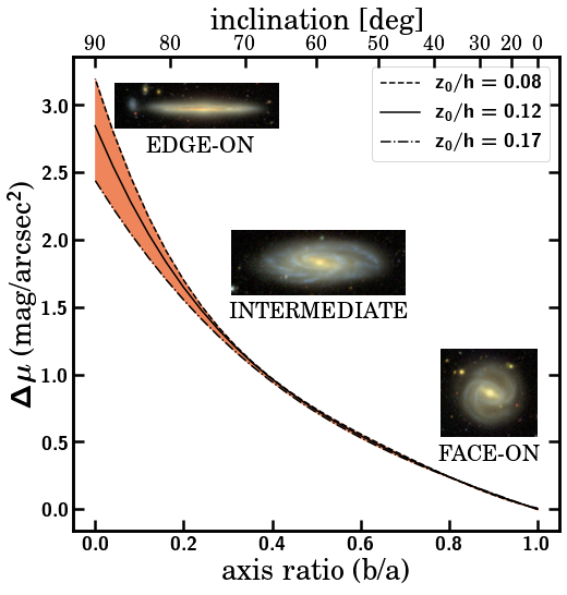
Figure 1: Difference in surface brightness $\Delta\mu=\mu_{\rm face-on}-\mu_{\rm inc}$ between the face-on orientation and a given inclination for a disc-like galaxy. The figure shows $\Delta\mu$ along the semi-major axis of a galaxy model at a radial distance $R=5h$ and is explored for three different disc thicknesses (shown in the legend) parameterized using $z_{0}/h$.

Figure 1 shows that the difference in brightness $\Delta\mu$ produced by different disc thicknesses (as parameterized by $z_{0}/h$) is only noticeable at very large inclinations (i.e. $i>$70 degrees). For this reason, we remove any galaxy with an axis ratio smaller than 0.3 from the sample (Sec 4). To facilitate the reader with the application of this inclination correction, we provide in Table 1 the values of the coefficients of a polynomial fit to the different models shown in Fig. 1:

$$\Delta\mu=\sum_{j=0}^{4}\alpha_{j}(b/a)^{j}$$ (2)

with $b/a$=cos($i$), the ratio of the semi-minor to the semi-major axis of the isophote used to measured the inclination of galaxies. The polynomial fit we provide is very accurate, with an error in $\Delta\mu<0.01$ mag. In the next Section, we explain how to apply this correction to real data. In this work, we have used the correction corresponding to the ratio $z_{0}/h$=0.12.

Table 1: Values of the polynomial coefficients to correct the surface brightness profiles of disc-like galaxies for the inclination effect. The coefficients have been calculated for three different disc thicknesses which are parameterised by the ratio $z_{0}/h$. As we are interested in the effect of inclination on the intermediate and outer regions of galaxies, this correction has been estimated at a distance $R=5h$ (see text for details).

$z_{0}/h$	$\alpha_{0}$	$\alpha_{1}$	$\alpha_{2}$	$\alpha_{3}$	$\alpha_{4}$
0.08	3.195	-10.396	17.584	-16.033	5.657
0.12	2.845	-7.833	10.792	-8.482	2.679
0.17	2.440	-5.273	4.577	-1.932	0.185

5.3 Stellar mass density profiles

After the removal of scattered light and masking the images, we extract the surface brightness profiles of the galaxies in the g and r bands to obtain their stellar mass density profiles. The surface brightness profiles are obtained using elliptical apertures with a fixed centre, axis ratio $q$ and position angle (PA). As a first guess for the centre of the galaxies, we use the R.A. and Dec information provided by the SDSS catalogues.

To determine the axis ratio and PA, for each galaxy we use those pixels where the surface brightness is between 25 and 26 mag/arcsec² in the $g$-band. The spatial distribution of these pixels were fit to an ellipse. The PA (in degrees) is the angle between the semi-major axis and the horizontal axis, measured in the counter clockwise direction from the horizontal axis. The fit parameters (centre, axis ratio and PA) of the ellipses were then visually checked to ensure the outermost parts of the galaxies were characterised properly. If not, they are corrected accordingly. Once fixed, surface brightness profiles of the galaxies are extracted by averaging their flux over annuli parameterised by the fit ellipse. These profiles are extracted up to a radial distance of 200 arcsec which is well beyond the visual extension of our galaxies. This is crucial in order to retrieve a sensible characterisation of the outer part of galaxies, particularly when the criterion we are proposing in this work is based on the location of a low stellar mass density contour such as 1 $M_{\rm\odot}$ pc^-2.

Another important effect that must be accounted for when obtaining surface brightness profiles is defining the level of the background. Although the IAC Stripe82 images we have used are background subtracted, in some occasions the subtraction was not precise enough to be a reliable representation of the (local) surrounding background value of the galaxies (i.e. a slight under- or overestimation). For this reason, in order to have the most accurate background subtraction as possible, we followed the procedure developed by Pohlen & Trujillo (2006). The radial distance up to which the profiles have been extracted (i.e. 200 arcsec) is about two times the location of the isophote at 26.5 mag/arcsec² (r-band) in the case of ellipticals and three times for the spiral and dwarf galaxies. This allows us to determine the background brightness in regions very close to the galaxies by identifying the asymptotic value in the number of counts around the object. We fit that value, subtract/add it to the images and obtain the profile once more.

We then correct the surface brightness profiles for Galactic extinction. The extinction corrections A_g and A_r are obtained from NED taking into account the location of each galaxy on the sky (https://ned.ipac.caltech.edu/forms/calculator.html). Following this, the effect of the inclination (see Section 5.2) is corrected for spiral and dwarf galaxies as follows. For each galaxy we measure its inclination based on the axis ratio we have determined before. The inclination correction, $\Delta\mu$, is then directly applied to the derived surface brightness profiles. The same inclination correction is applied for both g and r profiles, therefore the colour radial profile of galaxies remains unaffected. Due to our limited photometric information, we do not attempt any correction for internal dust.

The final step is to obtain the stellar mass-to-light ratio ($M/L$) profile. Once the $M/L$ is known, the following equation (see e.g. Bakos et al., 2008):

$$\log\Sigma_{\star}=\log(M/L)_{\lambda}-0.4(\mu_{\lambda}-\mu_{\rm abs,\odot,\lambda})+8.629$$ (3)

where $\mu_{\rm abs,\odot,\lambda}$ is the absolute magnitude of the Sun at wavelength $\lambda$, is used to obtain the stellar mass density (in $M_{\rm\odot}$ pc^-2) as a function of the surface brightness.

To compute $M/L$, we followed the procedure described by Roediger & Courteau (2015). As a basis for our estimation, we used the $g-r$ colour and the surface brightness in the g-band. We use the parameters provided by Roediger & Courteau (2015) that correspond to the Bruzual & Charlot (2003, BC03) models and a Chabrier IMF (Chabrier, 2003).

Despite the obvious advantage of decreasing the effect of galactic dust by using the i-band instead of the bluer g and r bands, we prefer to use the latter filters to estimate our size indicator for two main reasons. Firstly, the sky brightness in the i-band is around two magnitudes brighter than in the g-band (see e.g. Fig. 1 in Hall et al., 2012). This effect is not compensated by the brighter emission of the stellar populations towards the red (which is typically between g-i=0.5 to 1 mag for spiral galaxies). As a result, the redder SDSS bands are noisier at a given surface brightness because all the SDSS bands have the same integration time. Secondly, as our size indicator is estimated through a colour combination, the effect of the PSF on the surface brightness profiles should not be very different from band to band. This applies for g and r, but in the case of the i-band, the SDSS PSF is significantly different for those in g and r, as can be seen in de Jong (2008, Figure 2) and Infante-Sainz et al. (2020, Figure 8).

5.4 Estimating the structural parameters of galaxies

Once the stellar mass density profiles of the galaxies are created, it is straightforward to obtain the total stellar mass and the location of $R_{\rm 1}$, the proxy for the location of the gas density threshold for star formation we have adopted as a measure of size in this work. This procedure has been performed for all the galaxies in our sample. In order to get a homogeneous determination of the total stellar mass of all our galaxies, we have integrated their mass density profiles. The integration takes into account the axis ratio of the galaxy and therefore assumes an elliptical symmetry for the distribution of light, from the central position of the object up to the radial location provided by the 29 mag/arcsec² isophote (g-band). This estimate of the total stellar mass is a lower limit to the total mass of the object. However, the limiting isophote we are using is extremely faint, therefore the amount of stellar mass beyond such an isophote is expected to be very low ($<$3%; Trujillo et al., 2001). We prefer to use this approach for estimating the total stellar mass instead of assuming a shape for the light distribution (i.e. exponential, de Vaucouleurs, etc) and extrapolating the stellar mass density profiles to infinity. In Appendix D, we compare our stellar mass determination with that of the Portsmouth Spectro-Photometric Stellar Mass computation (Maraston et al., 2013) and find that both mass determinations are similar. Finally, we determine the location of $R_{\rm 1}$ directly using the stellar mass density profiles. Estimates of the half-mass radii are done using the cumulative mass density profiles.

The effective radii of galaxies are determined from the g-band images (our deepest data). We use the growth curve in g to obtain the radial location within which half of the total light of the galaxy is contained. As we have done for the total stellar mass, the total light of the galaxy is measured as the light enclosed by the observed 29 mag/arcsec² isophote (g-band). By definition, $R_{\rm e}$ is not affected by Galactic extinction nor the inclination correction of the profiles except indirectly for the location of the 29 mag/arcsec² isophote (g-band). In addition, we also estimate the Holmberg Radius ($R_{\rm H}$) for all our galaxies. Lacking the B-band in our survey, the location of the observed isophote at $\mu_{g}$=26 mag/arcsec² was considered as a proxy for $R_{\rm H}$. Using the i-band profiles, we also determine the radial location of the isophote corresponding to 23.5 mag/arcsec² (i.e. $R_{\rm 23.5,i}$). Both isophotal sizes were estimated after correcting the profiles for Galactic extinction and cosmological dimming. All these structural parameters of our galaxies are provided in Table 2.

Table 2: Characteristics of the galaxies used in this work. Unless explicitly stated otherwise, the quantities provided in this table have been derived in this work. This table includes the name of the galaxies (Abolfathi et al., 2018), their spatial location (Abolfathi et al., 2018), their axis ratio ($q$) and the position angle of the ellipses (PA) used to extract the surface brightness profiles (measured counter-clockwise starting from the horizontal axis), Galactic extinctions in the g, r and i bands (from NED), spectroscopic redshift ($z$) (Abolfathi et al., 2018), morphological type (Nair & Abraham, 2010, TType=-99 corresponds to dwarf galaxies), effective radius $R_{\rm e}$ (measured in the g-band), the half-mass radius ($R_{\rm e,M_{\star}}$), the radius corresponding to the location of the isophote with $\mu_{i}$=23.5 mag/arcsec² (i.e. $R_{\rm 23.5,i}$), the Holmberg Radius ($R_{\rm H}$), the radial location $R_{\rm 1}$ of the isomass contour at 1 $M_{\rm\odot}$ pc ^-2 and the stellar mass of galaxies (assuming a Chabrier IMF). The quantities are given showing only the significant figures up to which the values can be regarded reliable. The table shows those galaxies in Fig. 2 and 3, in order of appearance. The complete table is available in the online version of the paper.

JID	R.A.	Dec	$q$	PA	Ag	Ar	Ai	$z$	TType	$R_{\rm e}$	$R_{\rm e,M_{\star}}$	$R_{\rm 23.5,i}$	$R_{\rm H}$	$R_{\rm 1}$	Log(M⋆/$M_{\rm\odot}$)
	(deg)	(deg)		(deg)	(mag)	(mag)	(mag)			(kpc)	(kpc)	(kpc)	(kpc)	(kpc)
J010301.72-010639.46	15.75723	-1.11113	0.88	95.0	0.134	0.093	0.069	0.0175	-2	2.45	3.67	7.94	11.67	18.56	10.38
J005753.69-004852.90	14.47382	-0.81479	0.96	120.0	0.094	0.065	0.048	0.0419	-2	2.78	4.47	12.41	17.27	25.08	11.03
J000150.32+010155.24	0.45973	1.03172	0.49	179.0	0.085	0.059	0.044	0.0862	-5	24.99	29.13	46.05	71.98	148.12	11.82
J003934.82+005135.83	9.89529	0.85979	0.71	61.0	0.066	0.046	0.034	0.0146	5	8.64	7.70	16.39	20.87	23.01	10.37
J012223.77-005230.73	20.59913	-0.87523	0.44	42.0	0.169	0.117	0.087	0.0271	4	16.17	9.65	32.27	44.35	44.04	10.96
J021219.69-004841.46	33.08210	-0.81153	0.89	37.0	0.097	0.067	0.050	0.0408	0	9.18	5.90	23.68	32.61	37.17	11.24
J021808.12+004529.8	34.53385	0.75830	0.64	133.0	0.130	0.090	0.067	0.0092	-99	1.00	1.49	1.79	2.86	2.97	8.05
J233646.86+003724.2	354.19526	0.62341	0.86	88.0	0.113	0.078	0.058	0.0088	-99	2.13	2.38	2.58	4.44	5.44	8.65
J010607.19+004633.5	16.52997	0.77599	0.84	48.0	0.084	0.058	0.043	0.0174	-99	5.43	5.21	4.14	10.87	10.91	9.10
J235618.80-001820.17	359.07860	-0.30583	0.71	99.0	0.124	0.086	0.064	0.0241	-3	4.11	5.08	16.70	26.56	48.39	11.15
J024331.30+001824.49	40.88040	0.30676	0.36	108.0	0.124	0.086	0.064	0.0267	3	8.82	5.72	22.89	30.75	29.43	10.57

6 Results

Figure 2 shows a few representative galaxies in our sample to illustrate the difference between the location of their $R_{\rm 1}$ and $R_{\rm e}$ contours. The size based on the location of the gas density threshold for star formation much better represents the intuitive concept of the size of galaxies, such as its edge or boundary compared to $R_{\rm e}$. Expanding on this point, Fig. 3 shows the location of $R_{\rm 1}$ and $R_{\rm e}$ for two galaxies with clear signatures of on-going stellar accretion. In these examples, the location of $R_{\rm 1}$ may serve as a marker to separate the stellar material which is in the form of streams (formed ex-situ) from those stars which are located in the bulk (in-situ) of the main galaxy. An in-depth analysis of the use of $R_{\rm 1}$ (and its variants) for this purpose will be presented in a future publication (N. Chamba et al. in prep).

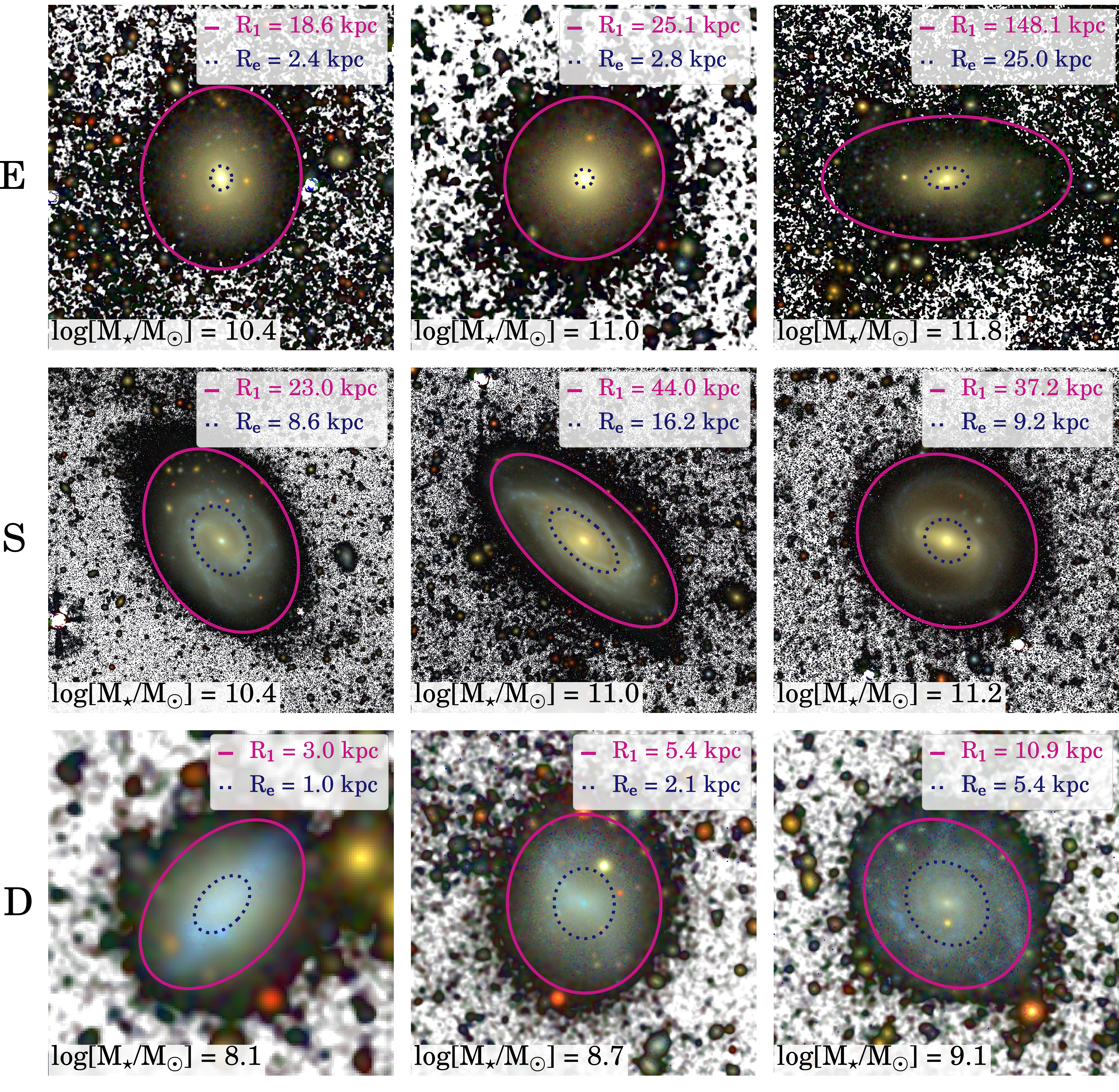
Figure 2: Collection of galaxy images showing the location of their $R_{\rm e}$ and $R_{\rm 1}$, the isomass contour at 1 $M_{\rm\odot}$ pc^-2. The top row shows galaxies which have been classified as ellipticals (E0-S0+), the middle row shows spiral (S0/a-Sm) galaxies, and the lower row shows dwarf galaxies. The galaxies are displayed with increasing stellar mass from left to right. This figure clearly illustrates how the proxy for the gas density threshold for star formation ($R_{\rm 1}$) nicely encloses the bulk of the stellar mass of galaxies. The coloured regions of the images are the IAC Stripe82 g, r and i band composite, while the black and white background is the sum of the 3 bands. The background level of these images is $\sim$29.1 mag/arcsec² (3$\sigma$ 10$\times$10 arcsec²; r-band). Table 2 lists details of the galaxies shown.

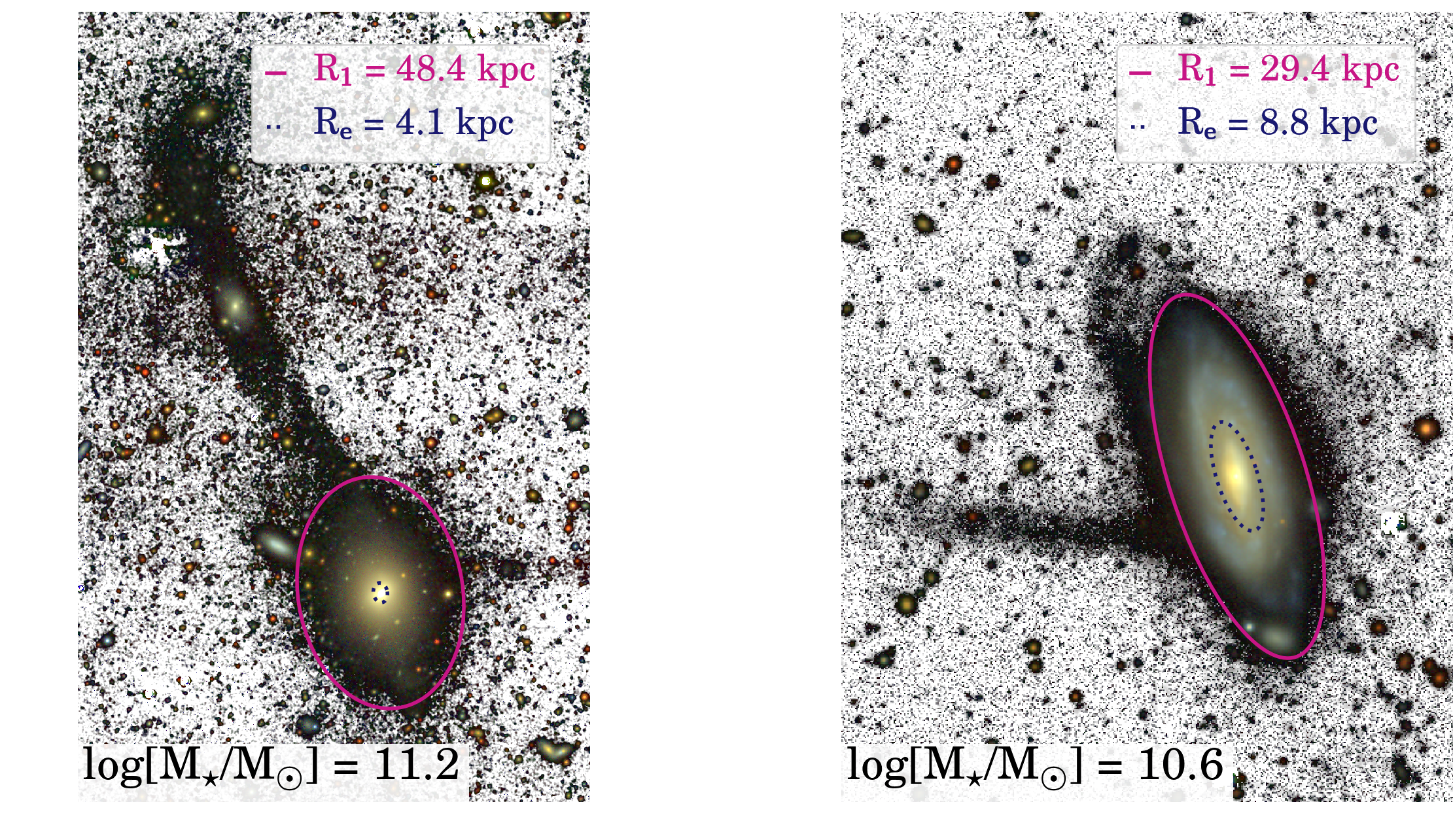
Figure 3: Separating in-situ star formation from ex-situ stellar accretion using our size measure (see N. Chamba et al. in prep. for further details). The two images show how the isomass contour at 1 $M_{\rm\odot}$ pc^-2 (i.e. $R_{\rm 1}$ or the proxy for the location of the gas density threshold for star formation) nicely divides the structure of galaxies into two different parts: the inner region where the bulk of the stars is contained and where in-situ star formation is or has been taking place and the external region where streams of on-going accretion are clearly visible. The left panel shows a massive elliptical and the right panel corresponds to a spiral galaxy with similar stellar mass to the Milky Way. See Table 2 for details on the galaxies shown.

6.1 The properties of the $R_{\rm 1}$ - mass relation

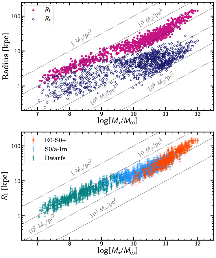
Figure 4: Stellar mass - size relation for the galaxies in our sample. Upper panel: The observed $R_{\rm 1}$ - mass and $R_{\rm e}$ - mass relations, where $R_{\rm e}$ has been measured using the g-band. The scatter of the relation using $R_{\rm 1}$ is significantly smaller compared to that with $R_{\rm e}$. Lower panel: The same $R_{\rm 1}$ - mass relation after splitting our sample into three categories: ellipticals (E0-S0+), spirals (S0/a-Im) and dwarfs as labelled in the legend. Spiral and dwarf galaxies follow the same trend, while massive ellipticals with $M_{\star}$>10¹¹ $M_{\rm\odot}$ show a tilt with respect to less massive galaxies. The grey dashed lines correspond to locations in the plane with constant (projected) stellar mass density.

The main result of this paper is shown in Fig. 4: the mass - size relation spanning over five orders of magnitude in stellar mass (10⁷-10¹² $M_{\rm\odot}$). The figure illustrates how the mass - size relation changes when using $R_{\rm 1}$ instead of $R_{\rm e}$ as a size measurement of galaxies. To extract both the slope and dispersion of the relations, we used a Huber Regressor (Huber, 1964), which is a linear regression model that is robust to outliers. We list a number of enlightening results:

• $R_{\rm 1}$ is a factor of 5 to 10 larger than $R_{\rm e}$ in all galaxies.

• The observed scatter of the stellar mass - size relation is significantly lower by a factor of $\sim$2 (from $\sigma_{\rm R_{e}}$$\sim$0.17 dex to $\sigma_{R_{1}}$$\sim$0.09 dex) compared to the scatter using $R_{\rm e}$ as a size indicator. As we will show in the next section, once the observational and methodological uncertainties are accounted for, the scatter of the stellar mass - size relation drops even more to a tiny 0.06 dex (i.e. a factor of $\sim$2.5 smaller than the intrinsic scatter using $R_{\rm e}$). The observed global scatter of the R1 - mass size relation is also lower than the observed one found using other popular size estimators ($\sigma_{R_{e,M_{\star}}}$$\sim$0.12 dex, $\sigma_{R_{H}}$$\sim$0.11 dex and $\sigma_{R_{23.5,i}}$$\sim$0.11 dex; see Table 3).

• The average 2D stellar density (as measured within $R_{\rm 1}$) changes from $\sim$10 $M_{\rm\odot}$ pc^-2 for the less massive galaxies to $\sim$100 $M_{\rm\odot}$ pc^-2 for the most massive spiral galaxies. Above 10¹¹ $M_{\rm\odot}$, the average 2D stellar density of the galaxies decreases again.

• From 10⁷ to 10¹¹ $M_{\rm\odot}$ all galaxies are located on the same mass - size relation following a power law, $R_{\rm 1}$$\propto$M_⋆^β, with $\beta$=0.35$\pm$0.01. This value is compatible with the one found by Hall et al. (2012) who compared the disc scale lengths of spiral galaxies with their luminosities and found $\beta$=0.377$\pm$0.007. Interestingly, $\beta\sim$1/3 would correspond to almost the same 3D stellar mass density ($\sim$4.5$\times$10^-3 $M_{\rm\odot}$ pc^-3) if all the stars were distributed in a sphere of radius $R_{\rm 1}$.

• Above 10¹¹ $M_{\rm\odot}$, the slope of the relation rises to $\beta$=0.58$\pm$0.02. This likely indicates that the most massive galaxies have formed or gained their stars very differently compared to galaxies with lower masses.

In Table 3 we show the best-fit parameters to a power law of the form R$\propto$M${}_{\star}^{\beta}$ using all the galaxies in the size - stellar mass relation as well as separate fits using each subsample (i.e. dwarfs, S0/a-Sm and E0-S0+). We have performed our analysis using the new size indicator $R_{\rm 1}$ as well as other popular size indicators: $R_{\rm e}$, $R_{\rm e,M_{\star}}$, $R_{\rm H}$ and $R_{\rm 23.5,i}$. The uncertainties in the best fit slope $(\beta)$ and dispersion of the observed relations ($\sigma_{\rm R_{obs}}$) are computed using a simple bootstrap method. One third of the measured points on the relation were randomly selected and fit at each iteration, for 1000 iterations. The spread in the distribution of the fits from this exercise is what is reported as the uncertainty in $\beta$ and $\sigma$. As we mentioned above, the observed global scatter of the $R_{\rm 1}$ - mass relation is significantly smaller than the one observed using $R_{\rm e}$ and lower than the observed scatter with all other size estimators, i.e. $R_{\rm e,M_{\star}}$, $R_{\rm H}$ and $R_{\rm 23.5,i}$. The values of the scatter in the size - mass relations are, however, affected by uncertainties in estimating the stellar mass and the background around the galaxies. In order to quantify how these uncertainties affect the observed scatter of the different relations and therefore compare the intrinsic scatter of the relation using $R_{\rm 1}$ with the other size indicators, we have conducted a number of tests which we describe in the next subsection.

Table 3: Best fit power law slope $\beta$ and the observed dispersion of different size - mass relations. We provide the values for the entire sample as well as for the different families of galaxies. The third column corresponds to the Pearson r correlation coefficient. We also calculate the contribution to the observed scatter produced by the uncertainty in the background of the images ($\sigma_{\rm R_{back}}$) and in our stellar mass estimation ($\sigma_{\rm R_{mass}}$). The last column shows the intrinsic scatter of the size - mass relation ($\sigma_{\rm R_{int}}$) after accounting for the uncertainty in the background and the stellar mass of the objects.

Galaxy Type	$\beta$	$\sigma_{\rm R_{obs}}$	r	$\sigma_{\rm R_{back}}$	$\sigma_{\rm R_{mass}}$	$\sigma_{\rm R_{int}}$
			$R_{\rm 1}$-stellar mass
All	0.365$\pm$0.005	0.089$\pm$0.005	0.971	0.045$\pm$0.003	0.047$\pm$0.003	0.061$\pm$0.005
E0-S0+	0.580$\pm$0.022	0.090$\pm$0.006	0.936	0.060$\pm$0.004	0.054$\pm$0.004	0.040$\pm$0.006
S0/a-Sm	0.332$\pm$0.014	0.089$\pm$0.005	0.881	0.045$\pm$0.003	0.035$\pm$0.002	0.068$\pm$0.005
Dwarfs	0.362$\pm$0.016	0.088$\pm$0.006	0.931	0.020$\pm$0.003	0.056$\pm$0.006	0.065$\pm$0.006
			$R_{\rm e}$-stellar mass
All	0.247$\pm$0.011	0.168$\pm$0.009	0.811	$\sim$0.001	0.067$\pm$0.005	0.154$\pm$0.009
E0-S0+	0.553$\pm$0.032	0.108$\pm$0.009	0.894	$\sim$0.001	0.092$\pm$0.006	0.057$\pm$0.009
S0/a-Sm	0.225$\pm$0.026	0.162$\pm$0.009	0.556	$\sim$0.001	0.047$\pm$0.002	0.155$\pm$0.009
Dwarfs	0.283$\pm$0.040	0.221$\pm$0.012	0.621	$\sim$0.001	0.064$\pm$0.004	0.212$\pm$0.012
			$R_{\rm e,M_{\star}}$-stellar mass
All	0.204$\pm$0.006	0.117$\pm$0.008	0.854	$\sim$0.001	0.052$\pm$0.003	0.105$\pm$0.008
E0-S0+	0.509$\pm$0.021	0.086$\pm$0.007	0.918	$\sim$0.001	0.075$\pm$0.006	0.042$\pm$0.007
S0/a-Sm	0.196$\pm$0.022	0.120$\pm$0.009	0.595	$\sim$0.001	0.040$\pm$0.002	0.113$\pm$0.009
Dwarfs	0.175$\pm$0.027	0.139$\pm$0.008	0.638	$\sim$0.001	0.038$\pm$0.003	0.134$\pm$0.008
			$R_{\rm H}$-stellar mass
All	0.304$\pm$0.007	0.109$\pm$0.005	0.940	0..003$\pm$0.001	0.056$\pm$0.004	0.094$\pm$0.005
E0-S0+	0.478$\pm$0.017	0.065$\pm$0.005	0.950	0.004$\pm$0.001	0.026$\pm$0.003	0.059$\pm$0.005
S0/a-Sm	0.266$\pm$0.014	0.105$\pm$0.005	0.783	0.003$\pm$0.001	0.035$\pm$0.004	0.099$\pm$0.005
Dwarfs	0.307$\pm$0.028	0.148$\pm$0.008	0.790	0.002$\pm$0.001	0.095$\pm$0.014	0.113$\pm$0.008
			$R_{\rm 23.5,i}$-stellar mass
All	0.330$\pm$0.006	0.106$\pm$0.006	0.944	0.002$\pm$0.001	0.062$\pm$0.005	0.086$\pm$0.005
E0-S0+	0.443$\pm$0.013	0.056$\pm$0.005	0.956	0.002$\pm$0.001	0.021$\pm$0.002	0.052$\pm$0.005
S0/a-Sm	0.285$\pm$0.016	0.104$\pm$0.006	0.804	0.003$\pm$0.001	0.052$\pm$0.005	0.090$\pm$0.006
Dwarfs	0.354$\pm$0.026	0.143$\pm$0.010	0.836	0.001$\pm$0.001	0.097$\pm$0.012	0.105$\pm$0.010

6.2 The intrinsic scatter of the $R_{\rm 1}$ - mass relation

There are two main sources of uncertainty which affect the observed scatter in the size - mass relations. The first is the accuracy in measuring the background level around the galaxies. For some galaxies (particularly the massive ellipticals or those with red stellar populations) the surface brightness at which $R_{\rm 1}$ is measured is very faint ($\mu_{g}\sim$28 mag/arcsec²) and therefore, a slight under- or over- subtraction of the background would bend the surface brightness profiles of these objects and move the location of $R_{\rm 1}$. To quantify how this can affect the position of $R_{\rm 1}$ and the rest of the size indicators, we have taken all our observed surface brightness profiles and randomly subtracted/added a number of counts compatible with the uncertainty in the background level around each galaxy. This variation of the background allows us to measure the variation in size for each galaxy which can then be used to estimate its contribution to the total observed dispersion in the size-mass plane. This contribution ($\sigma_{\rm R_{back}}$) is shown in Table 3. The background determination affects the size determination for massive ellipticals more than for spirals and/or small dwarfs. This is because the latter are mainly star-forming objects and therefore the surface brightness at which $R_{\rm 1}$ is located is brighter ($\mu_{g}$$\sim$26-27 mag/arcsec²). This explanation also applies for the isophotal sizes $R_{\rm H}$ and $R_{\rm 23.5,i}$. However, for $R_{\rm e}$ and $R_{\rm e,M_{\star}}$, the scatter due to the background correction is negligible.

The other significant source of scatter in the size - mass plane is the uncertainty in measuring the total stellar mass of galaxies from the integrated stellar mass density profile of the objects. As explained in Sect. 5.4, we measure our total stellar mass by integrating the stellar mass density profiles. To quantify how the uncertainty in the total stellar mass affects our results, we have assumed the following uncertainties in measuring the stellar mass: $\delta_{mass}$=0.24$\pm$0.01 dex (for the entire sample), $\delta_{mass}$=0.19$\pm$0.01 dex (for the E0-S0+ subsample), $\delta_{mass}$=0.24$\pm$0.01 dex (for the S0/a-Sm subsample) and $\delta_{mass}$=0.25$\pm$0.03 dex (for the Dwarfs subsample). These values were computed by an analysis of the differences between the Portsmouth stellar masses of our galaxies (Maraston et al., 2013) and those we measured using the g-r colour profile (Roediger & Courteau, 2015, see Appendix D for further details). To model the effect of the mass uncertainty ($\sigma_{\rm R_{mass}}$) on the scatter of the scaling relationship, all the observed stellar mass profiles were either scaled up or down in mass to place the galaxies on the best fit line through the observed stellar mass plane. This has been performed self-consistently, i.e. taking into account the change in the location of $R_{\rm 1}$ due to the scaling of the profile. Once all the galaxies are located exactly on top of the best-fit stellar mass - size relation (i.e. with zero scatter), we randomly scale the stellar mass density profiles up or down again, this time by a quantity compatible with a Gaussian distribution whose standard deviation is given by the above $\delta_{mass}$ values. We repeat this procedure 1000 times and on each occasion we measure the scatter of the stellar mass - size plane produced by the uncertainty in measuring the stellar mass. We show an illustration of the scatter of the stellar mass - size relation caused by the uncertainty in stellar mass in Fig. 10. The scatter in the stellar mass - size plane generated by the uncertainty in mass is shown in Table 3. Interestingly, for $R_{\rm 1}$, $R_{\rm H}$ and $R_{\rm 23.5,i}$, we find that the dwarfs are the most affected by the uncertainty due to our mass determination. This is once again expected as the star formation activity of dwarf galaxies is, on average, more stochastic (Kauffmann, 2014) and complicated to model than that of massive spirals and ellipticals. Therefore, a single colour is not a good proxy for the M/L ratio of dwarfs as it is in the case for more gentle star formation histories.

Once the scatter produced by both the uncertainty in the background and the stellar mass determination have been characterised, we can calculate the intrinsic scatter of the stellar mass-size relations. To do this, we have taken the observed scatter and removed in quadrature the two scatters generated by the background level and stellar mass uncertainty. Obviously, the exact intrinsic scatter of the mass - size relation is difficult to measure as there is some ambiguity in choosing the uncertainty in stellar mass. Here we have used the above uncertainty values in the stellar mass motivated by what we find comparing the Portsmouth stellar masses (Maraston et al., 2013) with the ones we retrieve using the g-r colour (Roediger & Courteau, 2015). We acknowledge that our intrinsic scatter values are an approximation, but do estimate that the intrinsic scatter of the $R_{\rm 1}$ - mass relation is about a factor of 1.5 smaller than the observed one (i.e. $\sim$0.06 dex), as a crude evaluation. This implies that the intrinsic stellar mass - $R_{\rm 1}$ relation is, indeed, very tight. In future work, we will address this issue in much more detail. This will be possible as a result of deeper data and therefore a decrease in the uncertainty in measuring the image background level. In addition, we plan to explore the stellar mass - $R_{\rm 1}$ relation using 3.6$\mu$m images (S. Díaz-García et al, in prep.) from Spitzer, where the uncertainty in measuring the stellar mass is smaller. In particular, we will use the S⁴G survey (Sheth et al., 2010) analysis where images have been corrected by the contamination from young stars (Querejeta et al., 2015) and the depth is enough to reach 1 $M_{\rm\odot}$ pc^-2 (Muñoz-Mateos et al., 2015).

Finally, it is worth mentioning how the intrinsic scatter of the new mass - size relation compares with the intrinsic scatter of the other popular size - mass relations. In the case of $R_{\rm e}$ and $R_{\rm e,M_{\star}}$, the uncertainty produced by an incorrect background determination is almost negligible. We have found for these cases that $\sigma_{R_{back}}\sim$0.001 dex. This is because our images are very deep and therefore the effect of the uncertainty in our background estimation on the surface brightness profiles barely affects the location of $R_{\rm e}$ and $R_{\rm e,M_{\star}}$ which are found at relatively high surface brightness values. Therefore, we do not expect a large contribution to the observed scatter of these size - mass relations from incorrect background level measurements. In the case of the uncertainty in stellar mass, the first thing to note is given that $R_{\rm e}$ ($R_{\rm e,M_{\star}}$) is defined as the location where half of the total light (stellar mass) is enclosed, its measurement is not affected by an incorrect mass determination of the object. This is because the only effect any uncertainty in mass could transfer to the shape of the profile is a scaling factor towards higher or lower stellar density. However, although the scatter in the size axis is negligible, the uncertainty in the mass axis will play a role in the total scatter of the size - mass plane. Nonetheless, there are two reasons why such an uncertainty will play a minor role in the observed scatter of these relations. Firstly, the slope of the $R_{\rm e}$ ($R_{\rm e,M_{\star}}$) - mass relation is rather flat in the region 10⁹ to 10¹¹ $M_{\rm\odot}$, therefore the contribution from an uncertainty in the mass to enlarge the scatter of the relationships in this region would be close to zero (for example, in spirals and $R_{\rm e}$, the observed scatter is $\sigma_{\rm R_{e}}$=0.162$\pm$0.009 while the intrinsic scatter is almost the same $\sigma_{\rm R_{e,int}}$=0.155$\pm$0.009). Secondly, as the observed scatters of the $R_{\rm e}$ ($R_{\rm e,M_{\star}}$) - mass relations are already larger than in the case of $R_{\rm 1}$ ($\sigma_{\rm R_{obs}}$), the contribution of a similar uncertainty in mass to the intrinsic scatter is very small. In the case of the $R_{\rm e}$-mass relation, as can be seen in Table 3, the global observed scatter is only reduced by 9% after accounting for the mass uncertainty, giving an intrinsic scatter of $\sigma_{\rm R_{e,int}}$=0.154$\pm$0.009. Therefore, it is reasonable to compare the scatter of the observed $R_{\rm e}$-mass relation with the intrinsic $R_{\rm 1}$-mass relation. As shown in Table 3, the decrease in scatter from $R_{\rm 1}$ to $R_{\rm e}$ ranges from a factor of 2.5 (comparing both intrinsic scatters) to 2.75 (comparing the intrinsic scatter using $R_{\rm 1}$ with the observed scatter using $R_{\rm e}$). We illustrate in Fig. 5 how the $R_{\rm 1}$ - mass relation would be observed without the scatter produced by the background level and the stellar mass determination. Finally, for the isophotal sizes $R_{\rm H}$ and $R_{\rm 23.5,i}$, the main contributor to the observed scatter is also the uncertainty in measuring the global mass of galaxies. In these cases, the intrinsic scatter for the global size - mass relation decreases by 15-20% compared to the observed values. Compared to the $R_{\rm 1}$ - mass relation, the intrinsic scatter of the global size - mass relations using $R_{\rm H}$ and $R_{\rm 23.5,i}$ is a factor of 1.5 and 1.4 larger, respectively. In Sec. 7.1, we expand on these results by comparing the scatter of the size - mass relations as a function of galaxy morphology.

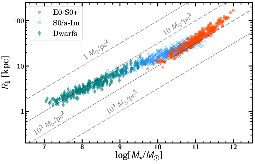
Figure 5: Similar to Fig. 4 (bottom panel), this figure shows the $R_{\rm 1}$–stellar mass relation as it would be observed without any uncertainty in measuring the background level of the images and the stellar mass of galaxies. The intrinsic scatter of the relation (0.06 dex) is a factor of 2.5 smaller than the scatter of the $R_{\rm e}$ - mass relation.

7 Discussion

The results of this paper show that the use of a physically motivated definition for the size of galaxies based on the location of the gas density threshold for star formation produces a global stellar mass - size relation with a very narrow intrinsic scatter (0.06 dex). In the following subsections, we compare the characteristics of the new size parameter $R_{\rm 1}$ as well as the $R_{\rm 1}$ - mass relation with other popular size measurements.

7.1 $R_{\rm 1}$ compared to other popular size definitions

In this paper we have used $R_{\rm 1}$ as a proxy for the location of the gas density threshold for star formation in galaxies. Nonetheless, the use of $R_{\rm 1}$ as a size indicator is reminiscent of definitions based on the B-band isophote at 25 mag/arcsec², at 26.5 mag/arcsec² (i.e. the Holmberg radius) or in the i-band such as $R_{\rm 23.5,i}$. Although our size definition is not based on the depth of current surveys (as was the case for the size parameters that were defined using photographic plates), it is worth exploring the stellar mass - size plane with popular isophotal size definitions. In this work we lack the B-band filter. As a compromise, we thus decided to use g-band imaging (the closest filter to the B-band with enough depth) available to us to show the stellar mass - size plane when using the position of the 26 mag/arcsec² (g-band) isophote as a size indicator. It is this isophote to which we refer to as the Holmberg radius ($R_{\rm H}$). We also include a comparison with size based on the location of the i-band isophote 23.5 mag/arcsec² ($R_{\rm 23.5,i}$). The results of this exercise are shown in Fig. 6.

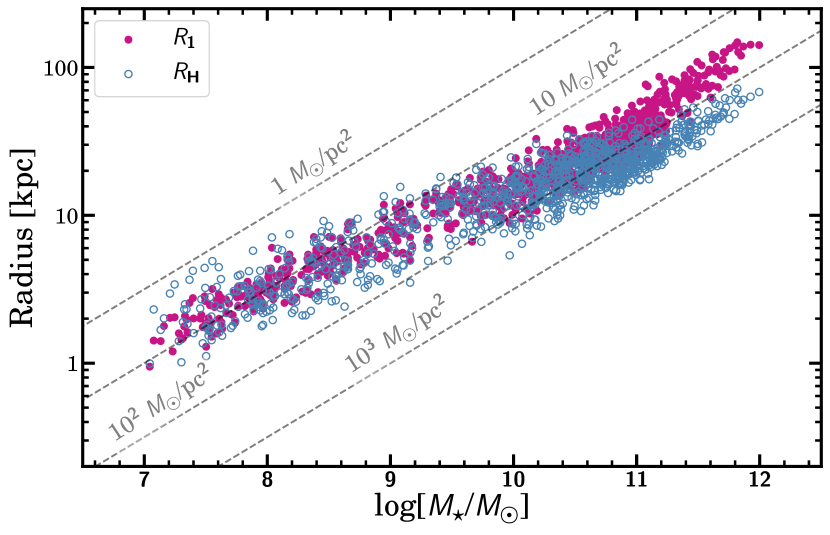
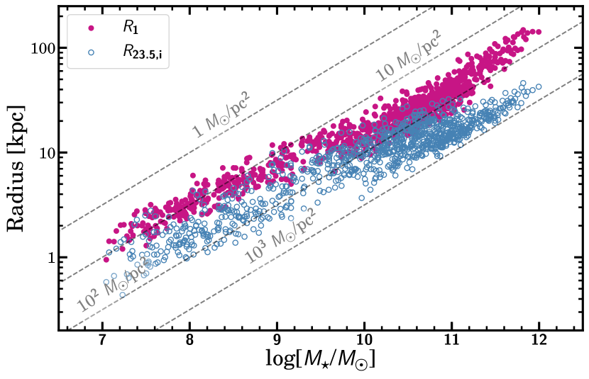
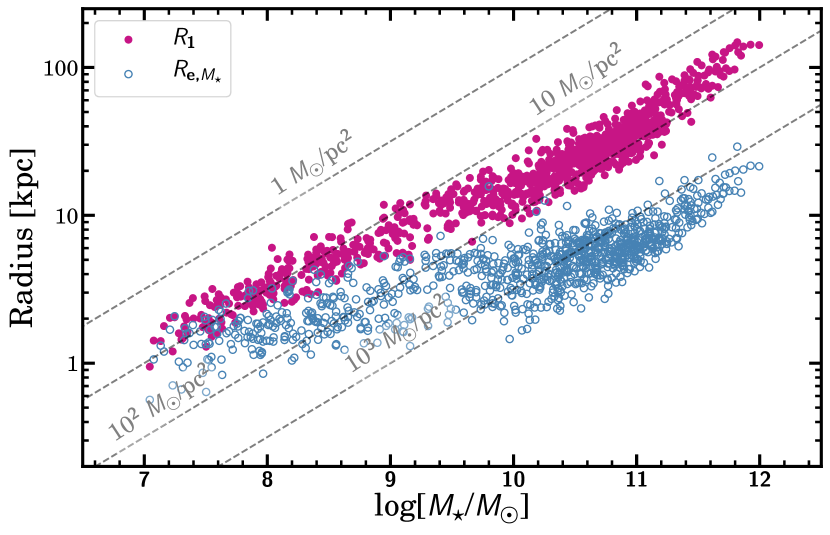
Figure 6: Comparing the $R_{\rm 1}$ - mass relation with other size - mass relations using: Holmberg Radius, $R_{\rm H}$ defined in this work as the 26 mag/arcsec^-2 isophote in SDSS g-band (upper panel), $R_{\rm 23.5,i}$, the radial location of the $\mu_{i}$=23.5 mag/arcsec² isophote (middle panel) and $R_{\rm e,M_{\star}}$, the half mass radius (lower panel).

The observed scatter of the global stellar mass - $R_{\rm H}$ relation is 0.109 $\pm$ 0.005. This value is larger than the one observed for $R_{\rm 1}$ (0.089$\pm$0.005). Interestingly, the scatter is particularly larger for the dwarfs and spirals than for the massive ellipticals. This is understandable as the variability in star formation activity among the less massive galaxies is larger than for the most massive ellipticals. Different star formation levels produce different $g$-band luminosities for the same stellar mass density, and therefore the scatter is larger when using size indicators based on blue bands (as is the case of $R_{\rm H}$). A potential way to decrease the scatter using a single photometric band would be to use a redder band (i.e. one less affected by recent star formation activity). For instance, one would expect the use of the i-band to decrease the scatter of the stellar mass - size relation. This is in fact the case. The observed scatter of the global stellar mass - $R_{\rm 23.5,i}$ relation is a bit lower (0.106 $\pm$ 0.006 dex) than in the case of $R_{\rm H}$ using the g-band.

While the observed scatter of the $R_{\rm 1}$-mass relation is predominantly affected by the uncertainty in background and mass estimation, in the case of the $R_{\rm H}$-mass and $R_{\rm 23.5,i}$-mass relations, the main contributor to the scatter is the mass uncertainty. This is because the 26 mag/arcsec² isophote in the g-band and the 23.5 mag/arcsec² in the i-band are brighter than the typical brightness of the isomass contour 1 $M_{\rm\odot}$ pc^-2 (see Sec. 6.2). Consequently, the contribution of the uncertainty in the background to the estimation of the location of $R_{\rm H}$ (and $R_{\rm 23.5,i}$) is not very important. Therefore, while the intrinsic scatter of the $R_{\rm 1}$-mass relation is around 0.06 dex, for $R_{\rm H}$-mass (and $R_{\rm 23.5,i}$ - mass) the global intrinsic scatter decreases to $\sim$0.09 dex. We discuss our findings in the context of the Hi - mass relation of galaxies in Appendix E.

Although the global size - mass relation using $R_{\rm 1}$ produces the smallest scatter, it is worth checking whether this is also the case for different galaxy families. The family of galaxies that consistently shows both the lowest observed and intrinsic scatter values in the stellar mass - size plane is the E0-S0+ group. This applies to all the size indicators explored, including the effective and half-mass radii. It is particularly remarkable that the observed scatter using $R_{\rm 23.5,i}$ (0.056$\pm$0.005 dex) is almost comparable to the lowest intrinsic scatter values obtained for this galaxy type using $R_{\rm 1}$ and the half-mass radius ($\sim$0.04 dex). The small scatter of the elliptical galaxies is a direct consequence of their low level of internal structure compared to other galaxies. This fact makes the members of this family almost homologous. Therefore, if one is interested in a relative comparison between the size of galaxies within such a family, any size indicator already suggested in the literature is useful.

In the case of the S0/a-Sm family, i.e. those galaxies with very complex internal structure consisting of bars, rings, spiral arms, etc, the difference in scatter among the size indicators is much larger than for the ellipticals. As expected, the size indicators showing the larger scatter for this galaxy type are those which better reflect the light concentration of the objects: i.e. the effective and the half-mass radii. However, those size measurements that are closer to a characterisation of the boundaries of the galaxies (e.g. $R_{\rm 1}$, $R_{\rm H}$ and $R_{\rm 23.5,i}$) are the ones with lower scatter. A similar result is found for the dwarf galaxies.

In addition to the above results, we also quantitatively compare the scatters found here for spiral galaxies with those measured in the literature. Similar to Saintonge & Spekkens (2011) and Hall et al. (2012), we divide our spiral galaxy sample into three categories: Sa-Sab, Sb-Sbc and Sc-Sd. In Fig. 7 we show the stellar mass - size relations for these types using $R_{\rm 1}$ and R_23.5i as size indicators. We find a similar stratification as the one reported by Saintonge & Spekkens (2011), Hall et al. (2012) and Muñoz-Mateos et al. (2015), i.e. at fixed stellar mass (or luminosity), those galaxies having later types are the largest. This is especially manifested at the low mass end. Saintonge & Spekkens (2011) has a sample mostly composed of Sc galaxies. Using R_23.5i and the luminosity in the i-band, they found an observed scatter of 0.05 dex. For the same morphological type, we find here (this time using the stellar mass) an observed scatter of 0.101$\pm$0.007 dex. The larger scatter is connected to the fact that we use the stellar mass instead of the luminosity. The observed scatter using $R_{\rm 1}$ for Sc-Sd galaxies is 0.082$\pm$0.007 dex. As our main source of the scatter is the determination of the stellar mass, it is worth giving the intrinsic scatter values: 0.096$\pm$0.007 dex (R_23.5i) and 0.066$\pm$0.007 dex ($R_{\rm 1}$). Within the common mass range 10^9.5-10¹¹ $M_{\rm\odot}$ for all the spiral galaxy types, the observed scatters for the Sc-Sd galaxies are: 0.095$\pm$0.008 dex (R_23.5i) and 0.077$\pm$0.008 dex ($R_{\rm 1}$). The scatter reported by Saintonge & Spekkens (2011) is extraordinarily tight. Using a similar sample, Hall et al. (2012) found an observed scatter value for the R_23.5i-mass relation which ranges from 0.070 dex (for their higher quality sample) to 0.096 dex (their entire sample), which is in closer agreement with our observed value.

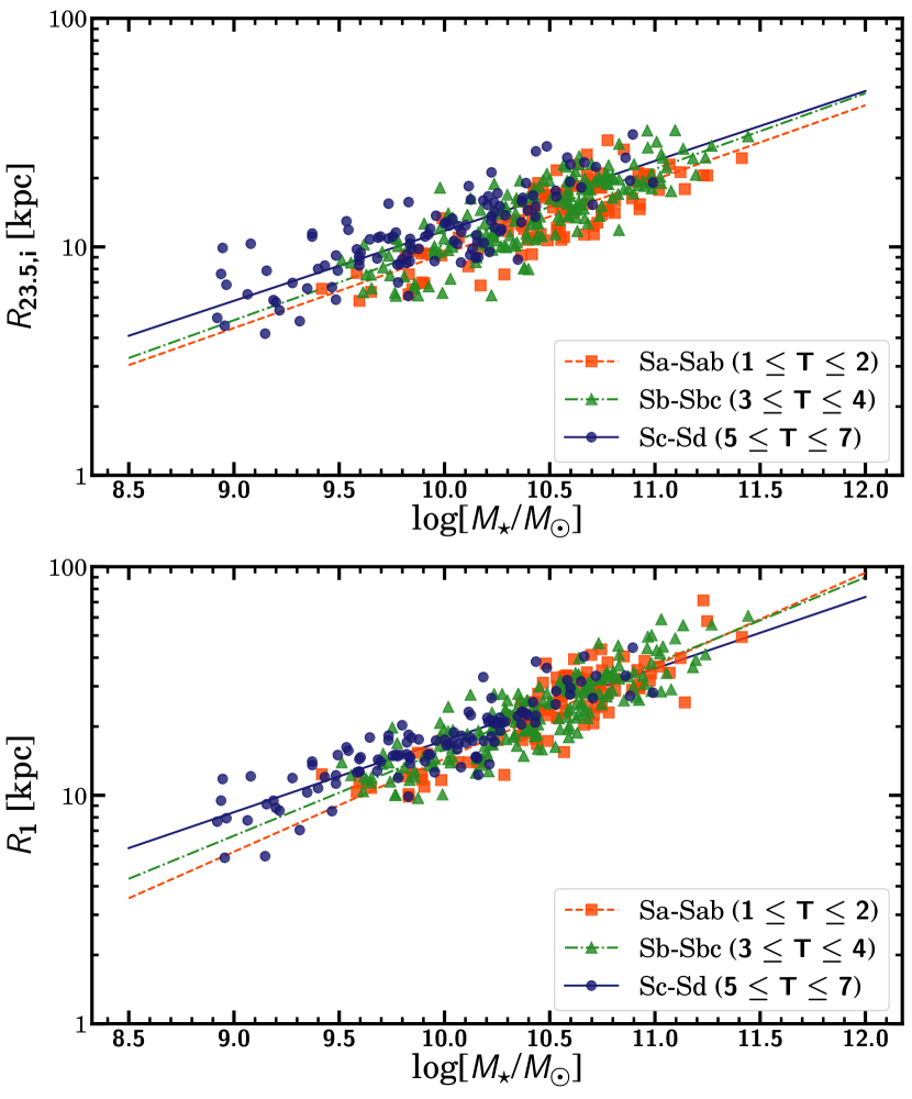
Figure 7: Stellar mass - size relation for three morphological groups within our spiral galaxy sample: Sa-Sab (orange squares), Sb-Sbc (green triangles) and Sc-Sd (blue dots). The top panel shows the relation using $R_{\rm 23.5,i}$ while the bottom panel shows the same relation using $R_{\rm 1}$ as the size indicator. Similar to Saintonge & Spekkens (2011), Hall et al. (2012) and Muñoz-Mateos et al. (2015), we find that spiral galaxies are stratified, with the largest ones at fixed stellar mass being those of later morphological types.

Another aspect to highlight is the change in the global slope of the stellar mass - size relation as a function of the size indicators we have explored. Using $R_{\rm 1}$, we find a slope a bit above 1/3 between 10⁷ to 10¹¹ $M_{\rm\odot}$. This value is in line with the one found using isophotal radii ($R_{\rm H}$ abd $R_{\rm 23.5,i}$) as a size measure. The slopes, however, decrease significantly when using the effective and half-mass radii. We expand on the potential meaning of the slope we measure using $R_{\rm 1}$ in subsection 7.2.

7.2 The slope of the stellar mass - size relation

The slope of the stellar mass - size relation we report for galaxies within the mass range 10⁷ to 10¹¹ $M_{\rm\odot}$ is very close to 1/3. A straightforward calculation shows that if all the stars within $R_{\rm 1}$ were located within a sphere of such radius, the stellar mass density (in 3D) of all the galaxies in this mass range will be equivalent to $\sim$4.5$\times$10^-3 $M_{\rm\odot}$ pc^-3. Obviously, the spatial configuration of both dwarf and spiral galaxies is not spherical but disc-like. Nonetheless, it is suggestive to think that the gas that originally formed all these objects was in a spherical-like configuration at an early galaxy phase before its collapse to form the disc configuration. In other words, it is worth speculating whether the currently observed 3D stellar density for all the galaxies in our sample is a reflection of a common 3D gas density at an early phase (before collapsing) of our objects. In fact, this constant 3D stellar density could be linked with the expected constant density of dark matter haloes which formed at a given age of the Universe (see e.g. Mo et al., 1998).

It is also worth indicating that while we see a monotonic increase in the size of galaxies with stellar mass using $R_{\rm 1}$ (as well as for $R_{\rm H}$ and $R_{\rm 23.5,i}$), the same is not true for $R_{\rm e}$ or $R_{\rm e,M_{\star}}$. This is particularly manifested in the interval 10⁹ to 10¹¹ $M_{\rm\odot}$ in stellar mass where the increase in effective (or in the half-mass) radius of the (mostly) spiral galaxies is very modest. This mass range is where the bulges of spiral galaxies appear. What we are witnessing here is the enormous impact of using $R_{\rm e}$ (or $R_{\rm e,M_{\star}}$) for measuring sizes when a significant amount of the light (or stellar mass) of galaxies can be concentrated in the inner parts of galaxies with a bulge. This small increase in $R_{\rm e}$ (or $R_{\rm e,M_{\star}}$) between 10⁹ to 10¹¹ $M_{\rm\odot}$ is not a minor issue. As the vast majority of works aiming to understand the connection between the galaxy size and the dark matter halo properties use $R_{\rm e}$ as a size indicator (see e.g. Kravtsov, 2013; Jiang et al., 2019; Zanisi et al., 2020), the small increase in the effective radius in this mass range can hide a potential connection between the dark and the luminous component of the galaxies. In a companion paper (C. Dalla Vecchia et al. in prep.), we show that the use of $R_{\rm 1}$ permits the connection of both galaxy components directly, ultimately facilitating our understanding about how these objects form.

7.3 The tilt of the stellar mass - size relation at 10¹¹ $M_{\rm\odot}$

A notable feature of the new stellar mass - size relation is the change in slope observed at $\sim$10¹¹ $M_{\rm\odot}$. The slope changes from $\sim$1/3 to $\sim$3/5 (see Table 3) for the most massive galaxies. The abrupt change in slope is found in all the size indicators probed in this work. This $\sim$10¹¹ $M_{\rm\odot}$ stellar mass value marks the shift between objects with disc-like configuration to objects with a spherical symmetry. In addition, this is the stellar mass where the transition from rotationally to pressure-supported systems has been reported (see e.g. Emsellem et al., 2011).

As mentioned in Appendix A, we speculate that this change in slope is a manifestation of different gas density threshold values for star formation in galaxies that formed at high-$z$ could have had. Observational evidence has shown that the most massive galaxies underwent a huge burst of star formation at high-z with star formation rates reaching values $\gtrsim$1000 $M_{\rm\odot}$ yr^-1 (see e.g. Riechers et al., 2013). The high star formation rates these galaxies have undergone could have injected a lot of energy into the gas, thereby preventing the star formation at low mass densities and consequently increasing the gas density threshold for star formation. A remnant of this huge star formation burst is the core of these massive galaxies that later undergo important merger activity, creating their envelopes (see e.g. Trujillo et al., 2011; Ferreras et al., 2014; Buitrago et al., 2017).

In short, we speculate that the tilt we observe at $\sim$10¹¹ $M_{\rm\odot}$ in the new stellar mass - size plane is a reflection of a change in the gas density threshold for star formation when the bulk of the most massive galaxies originated.

8 Conclusions

We introduce a new approach to define the luminous size of galaxies, aiming to link size with the region where galaxies form stars. In order to make such a physically motivated size definition operative, we propose using the average radial location of the gas density threshold for star formation to measure this quantity. We suggest the use of the radial position of the isomass contour at 1 $M_{\rm\odot}$ pc^-2 (here referred to as $R_{\rm 1}$) as a proxy for measuring this threshold. This value is motivated by both theoretical and observational arguments. In particular, the density value found at the location of the truncation in galaxies similar to our own Milky Way.

When using $R_{\rm 1}$ as a size indicator for galaxies, the global scatter of the stellar mass - size relation explored over five orders of magnitude in stellar mass drops significantly, reaching a value of $\sim$0.06 dex. This value is 2.5 times smaller than the scatter measured using the effective radius ($\sim$0.15 dex) and 1.5 to 1.8 times smaller than those using other traditional sizes indicators such as $R_{\rm 23.5,i}$ ($\sim$0.09 dex), $R_{\rm H}$ ($\sim$0.09 dex) and $R_{\rm e,M_{\star}}$ ($\sim$0.11 dex).

Between 10⁷ and 10¹¹ $M_{\rm\odot}$, the slope of the stellar mass - size relation is very close to 1/3. In a 3D spherical distribution, this corresponds to a constant stellar density of $\sim$4.5$\times$10^-3 $M_{\rm\odot}$ pc^-3, which could be a reflection of a common gas density when the primordial gas collapsed to form stars. Beyond 10¹¹ $M_{\rm\odot}$, the stellar mass - size relation gets steeper, reaching a slope of $\sim$3/5. We speculate that this drastic increase in size of the most massive galaxies could be linked to its different star formation histories, reflecting that the gas density threshold for star formation was higher at the epoch of their main formation burst.

Appendix A Is 1 $M_{\rm\odot}$ pc^-2 a good proxy for the location of the gas density threshold for star formation along the 10⁷ to 10¹² $M_{\rm\odot}$ mass range?

In this paper we propose the radial position of the isomass contour at 1 $M_{\rm\odot}$ pc^-2 as a size indicator motivated by its proximity to the location of the gas density threshold for star formation in galaxies found theoretically (see e.g. Schaye, 2004) and because this value is representative of the location of the disc truncation in galaxies similar to the Milky Way (Martínez-Lombilla et al., 2019). However, this value is not guaranteed to be representative of the gas density threshold for star formation in galaxies with very different stellar mass (like dwarfs) or those who were formed during an enormous burst of star formation at high-$z$ (as is the case of the most massive ellipticals). In fact, there are some hints in our data indicating that a running gas density threshold for star formation could be more representative of the size of galaxies. Looking at Fig. 2, we can appreciate that while 1 $M_{\rm\odot}$ pc^-2 very well represents the size of spiral galaxies, the use of this value does not fully enclose the extension of dwarf galaxies. A potential explanation for this is that in the case of dwarf galaxies the gas density threshold for star formation is lower than in the case of more massive spirals, and therefore using, for instance, 0.3-0.5 $M_{\rm\odot}$ pc^-2 instead of 1 $M_{\rm\odot}$ pc^-2 could be a better proxy for measuring the size of these small systems. This idea of a lower gas density threshold for star formation for dwarf galaxies is observationally supported as on average their amount of H₂ compared to Hi (and therefore their star-forming efficiency) is lower than for larger mass systems (see e.g. Leroy et al., 2008; Huang et al., 2012).

On the other hand, the situation would be reversed in the case of massive elliptical galaxies where $R_{\rm 1}$ is a bit larger than the visual extent of these galaxies. The gas density threshold for star formation during its high-z formation could be larger than whatit is currently for the spiral galaxies. In the local Universe, for instance, it has been found that starburst galaxies have significantly enhanced star formation (Jaskot et al., 2015). In this case, using an isomass contour with a larger density value (i.e. $>$1 $M_{\rm\odot}$ pc^-2) as size could be a better option for these very massive galaxies. In fact, one of the most notable features of the stellar mass - size relation we have analysed is the change in slope of the relation for galaxies above 10¹¹ $M_{\rm\odot}$ in stellar mass (Sec 7.3). We believe that this could be an indication that the proxy we are using to calculate the location of the gas density threshold for star formation for galaxies (i.e. the isomass contour at 1 $M_{\rm\odot}$ pc^-2) can be slightly different for galaxies where the bulk of star formation occurred at high-$z$. For this reason, we have explored how the relation changes when we use an isomass contour at 3 $M_{\rm\odot}$ pc^-2 for the size of the most massive objects. We show the result of doing such an exercise in Fig. 8.

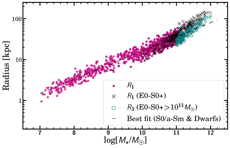
Figure 8: Stellar mass - size relation using different stellar mass densities as proxies for indicating the size of the most massive galaxies: $R_{\rm 1}$ and $R_{\rm 3}$. As can be seen, the size of the most massive objects changes depending on the isomass contour used to measure its size. The figure shows that most of the galaxies from 10⁷ to 10¹² could be allocated in the same stellar mass-size relation (i.e. with a similar slope) if $R_{\rm 3}$ were used for measuring the size of the galaxies for objects with stellar mass larger than 10¹¹ $M_{\rm\odot}$.

Using $R_{\rm 3}$ instead of $R_{\rm 1}$ for the most massive galaxies decreases the size of these objects and thus follows the trend observed in $R_{\rm 1}$ for the less massive galaxies (M${}_{\star}<10^{11}$ $M_{\rm\odot}$) as marked by the best fit dashed line in Fig. 8. Beyond 10^11.4 $M_{\rm\odot}$, however, even with $R_{\rm 3}$ the galaxies are above this trend in $R_{\rm 1}$. This is suggestive of an even larger gas density threshold for star formation in these ultra massive objects. In Chamba et al. (2020), we describe the opposite exercise using the dwarf galaxies.

Appendix B Other potential size indicators based on the location of the gas density threshold for star formation

Intimately linked to the gas density threshold for star formation is the drop-off of galaxy profiles, both in the optical and in H${\sc\alpha}$. The position of a sharp decline in the optical profile, often referred to in the literature as breaks or truncations (see a discussion about this in Martín-Navarro et al., 2012), has been used to explore the cosmic size evolution of galaxies (Trujillo & Pohlen, 2005; Azzollini et al., 2008). Unfortunately, not all galaxies show a clear deviation from the exponential decline in their profiles that can be used to trace their sizes (Pohlen & Trujillo, 2006). In this paper, we have used the fact that for Milky Way-like galaxies, the truncation is found near a stellar mass density of $\sim$1 $M_{\rm\odot}$ pc^-2. However, we do not know whether this result also holds for galaxies of different stellar mass (see Appendix A). In a future paper, we will explore this issue with our sample by identifying the location of the truncations in the profiles of our galaxies and determining the values of the stellar mass densities at those positions.

In addition to the drop-off in the optical profile, many disc galaxies show a sharp decline in their H${\sc\alpha}$ profiles. The location of this truncation in H${\sc\alpha}$ is also considered a good indicator of the radial position of the gas density threshold for star formation in actively star forming galaxies (see e.g. Martin & Kennicutt, 2001). The H${\sc\alpha}$ emission is directly linked to the presence of massive O stars and therefore the presence of recent star formation. In this sense, the location of the truncation radius in H${\sc\alpha}$ could be a direct indicator of the position of the gas density threshold for star formation and consequently, a very good proxy for galaxy size.

Despite the obvious advantages of using H${\sc\alpha}$ profiles to derive the size of galaxies, there are a number of practical limitations to a massive use of this technique. First, to the best of our knowledge, there are currently no deep H${\sc\alpha}$ surveys covering a large area of the sky that allow us to make this analysis on all kinds of galaxies. Second, contrary to the use of a stellar mass isocontour as we have done in this paper, the use of H${\sc\alpha}$ will be restricted to only those galaxies that are currently forming stars. In addition, as is also the case in the optical, not all the disc galaxies show a clear feature in their profiles that can be associated to a sharp decline in on-going star formation (see e.g. Koopmann et al., 2006). Nonetheless, in those cases where the break radii of H${\sc\alpha}$ surface brightness profiles have been measured, a bimodal distribution has been found, with the majority of the galaxies showing breaks at 0.7 or 1.1 $R_{25}$ (Christlein et al., 2010). It remains to be explored whether the breaks in H${\sc\alpha}$ are at the same location as that of the truncations in the optical for large samples of galaxies.

Finally, though the presence of H${\sc\alpha}$ is a clear indication of recent star formation, the H${\sc\alpha}$ line is connected with the presence of stars massive enough to generate a Stroemgren sphere. However, it is easy to imagine (particularly in the outer parts of galaxies where the density is very low) star formation occurring at low levels without the formation of very massive stars. In such a case, where H${\sc\alpha}$ is no longer present, the UV emission could be used as an indicator of recent star formation. As mentioned before, it would be necessary to search for a clear feature that can be associated to a gas density threshold for star formation in a large number of galaxies and thus approach the issue of galaxy size and star formation activity from multiple perspectives.

Appendix C The limits of the new size definition

Our size definition is motivated by the location of the gas density threshold for star formation in galaxies. This definition is rather general and there is no reason why this could not be applied to any galaxy where in-situ star formation is present. However, in order to make our size definition operative, we have used the position of the stellar mass density contour at 1 $M_{\rm\odot}$ pc^-2. By taking this specific value, we are limiting ourselves to characterise only the size of objects whose maximum stellar mass density is $\gtrsim$1 $M_{\rm\odot}$ pc^-2. Therefore, we quantify the brightness of objects that can not be characterised with such a specific prescription.

Some old and metal-poor galaxies with central surface brightness $\mu_{g}(0)>$27 mag/arcsec² would have a maximum stellar mass density $<$1 $M_{\rm\odot}$ pc^-2 and therefore, they would be unable to have a size estimation based on our proposed isomass contour. As the surface brightness of galaxies is not usually reported by their central value but as the brightness averaged within their effective radius (i.e. $<\mu>_{e}$), we compute which $<\mu>_{e}$ limits our size measure $R_{\rm 1}$. This is done by using the relation between central surface brightness and the average surface brightness according to a Sérsic profile:

$$<\mu>_{e}=\mu(0)-2.5\log\frac{n\Gamma(2n)}{b_{n}^{2n}}$$ (4)

where $n$ is the Sérsic index of the model. For 0.5$<n<$2 (a typical range of variation of the Sérsic index for galaxies with very low surface brightness; see e.g. Román & Trujillo, 2017), this would imply that the use of $R_{\rm 1}$ is limited to galaxies with $<\mu>_{e}\lesssim$ 28-29 mag/arcsec². This surface brightness is extremely low, nonetheless the current faintest galaxies detected in our Local Group (see e.g. Fig. 7 in McConnachie, 2012) have such extreme brightness. This again reinforces the idea we mentioned in Appendix A that low mass systems have very low star formation efficiency and therefore a lower gas density threshold for star formation. Future ultra-deep imaging surveys would allow us to better calibrate the gas density threshold for star formation values for low dense systems. Nevertheless, our size definition could be readily adjusted to these extreme objects by using a lower mass density contour for characterising their sizes.

Appendix D Stellar mass determination

As explained in the main body of the paper, stellar masses of all galaxies were calculated using their stellar mass density profiles which were derived using the g-r colour profiles (Roediger & Courteau, 2015). In order to evaluate the reliability of this mass estimate, we have compared our stellar mass estimations with those obtained by the Portsmouth group (Maraston et al., 2013). To do that we have retrieved the stellar masses from the Portsmouth Spectro-Photometric Model Fitting catalogue available on the SDSS webpage. The Portsmouth stellar masses are calculated using the BOSS spectroscopic redshift, $Z_{\rm NOQSO}$ and u, g, r, i, z photometry by means of broad-band SED fitting of stellar population models. Two separate stellar mass calculations were conducted: one assuming a passive template and the other a star-forming template. The version we have used here is the star-forming template with a Kroupa IMF.

In Fig. 9, we show the comparison between the stellar masses estimated in this work and those obtained by the Portsmouth group (when available). The ratio of these two mass estimates is approximately described by a Gaussian distribution. We find a systematic offset in our mass estimates by a factor of 1.6 with respect to the Portsmouth masses. This offset could be due to multiple reasons - we are not using the same IMF nor the same aperture to estimate the total flux of the objects. However, for our paper, the most relevant aspect is not the offset but the scatter in the difference between the two mass measurements. We calculate this scatter by measuring the r.m.s. of the ratio between the two masses. For the total sample, the r.m.s. of this distribution is 0.24 dex. In addition to showing the distribution of the ratio between the two masses of the entire sample, we also overplot the distribution of the same ratio for the different galaxy subsamples defined in this work. We find that the r.m.s. of the subsample distributions are: 0.19 dex (E0-S0+), 0.24 dex (S0/a-Sm) and 0.25 (Dwarfs).

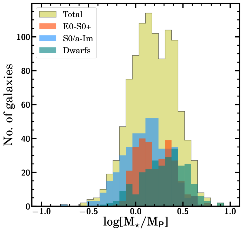
Figure 9: Uncertainty in measuring the stellar masses of galaxies used in our sample. $M_{\rm P}$ corresponds to the stellar mass of the objects reported by the Portsmouth group (Maraston et al., 2013) and $M_{\rm\star}$ is the mass we have estimated in this work using the g-r colour profile (Roediger & Courteau, 2015). We show the ratio of these two estimates for the full sample (yellow) and the different galaxy subsamples labelled in the legend.

In our analysis, we have used the above r.m.s. of the subsample distributions as a way of estimating the uncertainty in the stellar mass - size relation. In Fig. 10, we illustrate how the $R_{\rm 1}$ - mass relation with an intrinsic scatter equal to zero would look with only the uncertainty contribution from the stellar mass estimate. In other words, this plot shows the contribution of the mass uncertainty to the observed scatter of the mass - size relation. The scatter of the $R_{\rm 1}$-mass size relation plotted in Fig. 10, which is the scatter simply produced by the uncertainty in measuring the stellar mass, is $\sigma_{R_{1,mass}}$=0.047 dex. That is the contribution of the mass uncertainty to the total observed scatter of the $R_{\rm 1}$-mass size relation (i.e. $\sigma_{R_{1}}$=0.089 dex).

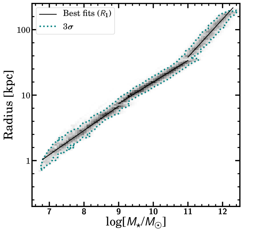
Figure 10: Scatter in the $R_{\rm 1}$-mass relation produced by the uncertainty in stellar mass. The figure shows how galaxies spread over the size - mass plane simply due to effect of the uncertainty in measuring the stellar mass of each galaxy. To build this plot we have assumed that the intrinsic scatter of the size - mass relation is exactly zero and follow how the uncertainty in measuring the mass will spread around the best fit lines to the observed measurements. The contour shows the 3 $\sigma$ distribution of the final sample.

Appendix E Comparing the $R_{\rm 1}$-stellar mass relation with the Hi size -mass relation of galaxies

An extremely tight scaling relation for galaxies is the one which links their total Hi mass with the diameter of their Hi discs defined by the location of the gas surface density at 1 $M_{\rm\odot}$ pc^-2 (Broeils & Rhee, 1997). This relation spans over five orders of magnitude in Hi mass. A subsequent analysis of this relation has shown that its scatter is extremely low: 0.06 dex and the slope almost exactly 1/2, i.e. 0.506$\pm$0.003 (Wang et al., 2016). These values are suggestive of a uniform characteristic Hi surface density of $\sim$5 $M_{\rm\odot}$ pc^-2.

In the case of the Hi size -mass relation of galaxies, the use of 1 $M_{\rm\odot}$ pc^-2 is a subjective choice and, contrary to the present work, there is no a priory physical motivation to select this value. Interestingly though, the scatter of the Hi size -mass relation is minimised when the Hi size is measured at surface densities between 1 to 2 $M_{\rm\odot}$ pc^-2.

The reason we cite this relation here is because of its potential connection to the size-mass relation we are exploring in this paper. In galaxy formation models (see e.g. Lagos et al., 2011), the Hi surface density is regulated by the conversion process from atomic to molecular hydrogen, i.e. Hi-to-H₂. Observationally, it is found that the Hi surface density saturates at $\sim$9 $M_{\rm\odot}$ pc^-2, and gas at higher surface densities are converted to molecular gas (Bigiel et al., 2008). As H₂ and star formation are closely linked (Krumholz et al., 2011), the Hi-to-H₂ process should be reflected in the star formation activity and, therefore, in the location of the gas density threshold for star formation in galaxies. As galaxies observationally have a very similar average Hi surface density of $\sim$5 $M_{\rm\odot}$ pc^-2 (as reflected by the tight Hi size - mass relation of galaxies), it seems reasonable to assume that the gas density threshold for star formation is also similar among very different galaxies. For this reason, we speculate that the small intrinsic scatter of the stellar mass - size relation we have explored in this work (based on the location of the gas density threshold for star formation) could be connected with or be a reflection of the tight Hi size - mass relation of galaxies.

References

- Abazajian et al. (2003) Abazajian K., et al., 2003, AJ, 126, 2081
- Abolfathi et al. (2018) Abolfathi B., et al., 2018, ApJS, 235, 42
- Aihara et al. (2018) Aihara H., et al., 2018, PASJ, 70, S4
- Azzollini et al. (2008) Azzollini R., Trujillo I., Beckman J. E., 2008, ApJ, 684, 1026
- Bakos et al. (2008) Bakos J., Trujillo I., Pohlen M., 2008, ApJ, 683, L103
- Bertin (2010) Bertin E., 2010, SWarp: Resampling and Co-adding FITS Images Together, Astrophysics Source Code Library (ascl:1010.068)
- Bigiel et al. (2008) Bigiel F., Leroy A., Walter F., Brinks E., de Blok W. J. G., Madore B., Thornley M. D., 2008, AJ, 136, 2846
- Bland-Hawthorn & Gerhard (2016) Bland-Hawthorn J., Gerhard O., 2016, ARA&A, 54, 529
- Borlaff et al. (2019) Borlaff A., et al., 2019, A&A, 621, A133
- Broeils & Rhee (1997) Broeils A. H., Rhee M. H., 1997, A&A, 324, 877
- Bruzual & Charlot (2003) Bruzual G., Charlot S., 2003, MNRAS, 344, 1000
- Buitrago et al. (2017) Buitrago F., Trujillo I., Curtis-Lake E., Montes M., Cooper A. P., Bruce V. A., Pérez-González P. G., Cirasuolo M., 2017, MNRAS, 466, 4888
- Camm (1950) Camm G. L., 1950, MNRAS, 110, 305
- Capaccioli et al. (2015) Capaccioli M., et al., 2015, A&A, 581, A10
- Chabrier (2003) Chabrier G., 2003, PASP, 115, 763
- Chamba et al. (2020) Chamba N., Trujillo I., Knapen J. H., 2020, A&A, 633, L3
- Christlein et al. (2010) Christlein D., Zaritsky D., Bland-Hawthorn J., 2010, MNRAS, 405, 2549
- Duc et al. (2015) Duc P.-A., et al., 2015, MNRAS, 446, 120
- Emsellem et al. (2011) Emsellem E., et al., 2011, MNRAS, 414, 888
- Erwin (2015) Erwin P., 2015, ApJ, 799, 226
- Fall & Efstathiou (1980) Fall S. M., Efstathiou G., 1980, MNRAS, 193, 189
- Ferrarese et al. (2012) Ferrarese L., et al., 2012, ApJS, 200, 4
- Ferreras et al. (2014) Ferreras I., et al., 2014, MNRAS, 444, 906
- Fliri & Trujillo (2016) Fliri J., Trujillo I., 2016, MNRAS, 456, 1359
- Fliri & Trujillo (2018) Fliri J., Trujillo I., 2018, VizieR Online Data Catalog, 745
- Freeman (1970) Freeman K. C., 1970, ApJ, 160, 811
- Frieman et al. (2008) Frieman J. A., et al., 2008, AJ, 135, 338
- Gaia Collaboration (2016) Gaia Collaboration 2016, VizieR Online Data Catalog, 1337
- Giovanelli et al. (1994) Giovanelli R., Haynes M. P., Salzer J. J., Wegner G., da Costa L. N., Freudling W., 1994, AJ, 107, 2036
- Graham (2019) Graham A. W., 2019, Publ. Astron. Soc. Australia, 36, e035
- Graham & Driver (2005) Graham A. W., Driver S. P., 2005, Publ. Astron. Soc. Australia, 22, 118
- Hall et al. (2012) Hall M., Courteau S., Dutton A. A., McDonald M., Zhu Y., 2012, MNRAS, 425, 2741
- Holmberg (1958) Holmberg E., 1958, Meddelanden fran Lunds Astronomiska Observatorium Serie II, 136, 1
- Holmberg (1975) Holmberg E., 1975, Magnitudes, Colors, Surface Brightness, Intensity Distributions Absolute Luminosities, and Diameters of Galaxies. p. 123
- Huang et al. (2012) Huang S., Haynes M. P., Giovanelli R., Brinchmann J., 2012, ApJ, 756, 113
- Huber (1964) Huber P. J., 1964, Ann. Math. Statist., 35, 73
- Hunter (2007) Hunter J. D., 2007, Computing in Science & Engineering, 9, 90
- Infante-Sainz et al. (2020) Infante-Sainz R., Trujillo I., Román J., 2020, MNRAS, 491, 5317
- Ivezic et al. (2008) Ivezic Z., et al., 2008, Serbian Astronomical Journal, 176, 1
- Jaskot et al. (2015) Jaskot A. E., Oey M. S., Salzer J. J., Van Sistine A., Bell E. F., Haynes M. P., 2015, ApJ, 808, 66
- Jiang et al. (2019) Jiang F., et al., 2019, MNRAS, p. 1977
- Jones et al. (2001) Jones E., Oliphant T., Peterson P., et al., 2001, SciPy: Open source scientific tools for Python, http://www.scipy.org/
- Kauffmann (2014) Kauffmann G., 2014, MNRAS, 441, 2717
- Kennedy et al. (2015) Kennedy R., et al., 2015, MNRAS, 454, 806
- Kennicutt (1989) Kennicutt Jr. R. C., 1989, ApJ, 344, 685
- Kluyver et al. (2016) Kluyver T., et al., 2016, in Loizides F., Schmidt B., eds, Positioning and Power in Academic Publishing: Players, Agents and Agendas. pp 87 – 90
- Knapen & van der Kruit (1991) Knapen J. H., van der Kruit P. C., 1991, A&A, 248, 57
- Kniazev et al. (2004) Kniazev A. Y., Grebel E. K., Pustilnik S. A., Pramskij A. G., Kniazeva T. F., Prada F., Harbeck D., 2004, AJ, 127, 704
- Koda et al. (2015) Koda J., Yagi M., Yamanoi H., Komiyama Y., 2015, ApJ, 807, L2
- Koopmann et al. (2006) Koopmann R. A., Haynes M. P., Catinella B., 2006, AJ, 131, 716
- Kourkchi et al. (2019) Kourkchi E., Tully R. B., Neill J. D., Seibert M., Courtois H. M., Dupuy A., 2019, arXiv e-prints, p. arXiv:1909.01572
- Kravtsov (2013) Kravtsov A. V., 2013, ApJ, 764, L31
- Kron (1980) Kron R. G., 1980, ApJS, 43, 305
- Krumholz et al. (2011) Krumholz M. R., Leroy A. K., McKee C. F., 2011, ApJ, 731, 25
- Lagos et al. (2011) Lagos C. D. P., Baugh C. M., Lacey C. G., Benson A. J., Kim H.-S., Power C., 2011, MNRAS, 418, 1649
- Leroy et al. (2008) Leroy A. K., Walter F., Brinks E., Bigiel F., de Blok W. J. G., Madore B., Thornley M. D., 2008, AJ, 136, 2782
- Liller (1960) Liller M. H., 1960, ApJ, 132, 306
- Maraston et al. (2013) Maraston C., et al., 2013, MNRAS, 435, 2764
- Martin & Kennicutt (2001) Martin C. L., Kennicutt Robert C. J., 2001, ApJ, 555, 301
- Martín-Navarro et al. (2012) Martín-Navarro I., et al., 2012, MNRAS, 427, 1102
- Martínez-Delgado et al. (2010) Martínez-Delgado D., et al., 2010, AJ, 140, 962
- Martínez-Lombilla et al. (2019) Martínez-Lombilla C., Trujillo I., Knapen J. H., 2019, MNRAS, 483, 664
- McConnachie (2012) McConnachie A. W., 2012, AJ, 144, 4
- Merritt et al. (2014) Merritt A., van Dokkum P., Abraham R., 2014, ApJ, 787, L37
- Mihos et al. (2017) Mihos J. C., Harding P., Feldmeier J. J., Rudick C., Janowiecki S., Morrison H., Slater C., Watkins A., 2017, ApJ, 834, 16
- Mo et al. (1998) Mo H. J., Mao S., White S. D. M., 1998, MNRAS, 295, 319
- Mo et al. (2010) Mo H., van den Bosch F. C., White S., 2010, Galaxy Formation and Evolution
- Möllenhoff (2004) Möllenhoff C., 2004, A&A, 415, 63
- Muñoz-Mateos et al. (2015) Muñoz-Mateos J. C., et al., 2015, ApJS, 219, 3
- Nair & Abraham (2010) Nair P. B., Abraham R. G., 2010, ApJS, 186, 427
- Oliphant (2006) Oliphant T., 2006, NumPy: A guide to NumPy, USA: Trelgol Publishing, http://www.numpy.org/
- Pedregosa et al. (2011) Pedregosa F., et al., 2011, Journal of Machine Learning Research, 12, 2825
- Petrosian (1976) Petrosian V., 1976, ApJ, 209, L1
- Pohlen & Trujillo (2006) Pohlen M., Trujillo I., 2006, A&A, 454, 759
- Price-Whelan et al. (2018) Price-Whelan A., et al., 2018, The Astronomical Journal, 156, 123
- Querejeta et al. (2015) Querejeta M., et al., 2015, ApJS, 219, 5
- Quirk (1972) Quirk W. J., 1972, ApJ, 176, L9
- Redman (1936) Redman R. O., 1936, MNRAS, 96, 588
- Riechers et al. (2013) Riechers D. A., et al., 2013, Nature, 496, 329
- Robitaille et al. (2013) Robitaille T. P., et al., 2013, Astronomy & Astrophysics, 558, A33
- Roediger & Courteau (2015) Roediger J. C., Courteau S., 2015, MNRAS, 452, 3209
- Román & Trujillo (2017) Román J., Trujillo I., 2017, MNRAS, 468, 703
- Román & Trujillo (2018) Román J., Trujillo I., 2018, Research Notes of the American Astronomical Society, 2, 144
- Saintonge & Spekkens (2011) Saintonge A., Spekkens K., 2011, ApJ, 726, 77
- Schaye (2004) Schaye J., 2004, ApJ, 609, 667
- Sersic (1968) Sersic J. L., 1968, Atlas de Galaxias Australes. Observatorio Astronomico, Universidad Nacional de Cordoba, 1968
- Sheth et al. (2010) Sheth K., et al., 2010, PASP, 122, 1397
- Slater et al. (2009) Slater C. T., Harding P., Mihos J. C., 2009, PASP, 121, 1267
- Smithsonian Astrophysical Observatory (2000) Smithsonian Astrophysical Observatory 2000, SAOImage DS9: A utility for displaying astronomical images in the X11 window environment, Astrophysics Source Code Library (ascl:0003.002)
- Spitzer (1942) Spitzer Jr. L., 1942, ApJ, 95, 329
- Spitzer (1968) Spitzer L., 1968, Diffuse matter in space. Interscience Publication, 1968
- Taylor (2005) Taylor M. B., 2005, in Shopbell P., Britton M., Ebert R., eds, Astronomical Society of the Pacific Conference Series Vol. 347, Astronomical Data Analysis Software and Systems XIV. p. 29
- Teeninga et al. (2016) Teeninga P., Moschini U., C. Trager S., Wilkinson M., 2016, 1
- Toth & Ostriker (1992) Toth G., Ostriker J. P., 1992, ApJ, 389, 5
- Trujillo & Fliri (2016) Trujillo I., Fliri J., 2016, ApJ, 823, 123
- Trujillo & Pohlen (2005) Trujillo I., Pohlen M., 2005, ApJ, 630, L17
- Trujillo et al. (2001) Trujillo I., Graham A. W., Caon N., 2001, MNRAS, 326, 869
- Trujillo et al. (2011) Trujillo I., Ferreras I., de La Rosa I. G., 2011, MNRAS, 415, 3903
- Tully & Fouque (1985) Tully R. B., Fouque P., 1985, ApJS, 58, 67
- Uson et al. (1991) Uson J. M., Boughn S. P., Kuhn J. R., 1991, ApJ, 369, 46
- Walt et al. (2011) Walt S. v. d., Colbert S. C., Varoquaux G., 2011, Computing in Science & Engineering, 13, 22
- Wang et al. (2016) Wang J., Koribalski B. S., Serra P., van der Hulst T., Roychowdhury S., Kamphuis P., Chengalur J. N., 2016, MNRAS, 460, 2143
- Zanisi et al. (2020) Zanisi L., et al., 2020, MNRAS, 492, 1671
- de Jong (2008) de Jong R. S., 2008, MNRAS, 388, 1521
- de Vaucouleurs (1948) de Vaucouleurs G., 1948, Annales d’Astrophysique, 11, 247
- de Vaucouleurs (1959) de Vaucouleurs G., 1959, Handbuch der Physik, 53, 275
- de Vaucouleurs et al. (1976) de Vaucouleurs G., de Vaucouleurs A., Corwin J. R., 1976, in Second reference catalogue of bright galaxies, Vol. 1976, p. Austin: University of Texas Press..