Coherent Quantum Channel Discrimination

Abstract

This paper introduces coherent quantum channel discrimination as a coherent version of conventional quantum channel discrimination. Coherent channel discrimination is phrased here as a quantum interactive proof system between a verifier and a prover, wherein the goal of the prover is to distinguish two channels called in superposition in order to distill a Bell state at the end. The key measure considered here is the success probability of distilling a Bell state, and I prove that this success probability does not increase under the action of a quantum superchannel, thus establishing this measure as a fundamental measure of channel distinguishability. Also, I establish some bounds on this success probability in terms of the success probability of conventional channel discrimination. Finally, I provide an explicit semi-definite program that can compute the success probability.

I Introduction

Quantum channel discrimination is a fundamental information-processing task in quantum information theory [1, 2, 3, 4, 5, 6, 7, 8]. There are at least two ways of thinking about it: one in terms of quantifying error between an ideal channel and an experimental approximation of it [1, 2] and another in terms of symmetric hypothesis testing [5, 6]. In both scenarios, the diamond distance between channels [1] arises as the fundamental metric quantifying the distinguishability of two quantum channels. These interpretations of diamond distance are the main reason that it is employed as the primary theoretical quantifier of channel distance in applications such as fault-tolerant quantum computation [9], quantum complexity theory [10], and quantum Shannon theory [11].

To expand upon the first way of thinking about channel discrimination from [1, 2], suppose that the ideal channel to be implemented is $\mathcal{N}_{A\rightarrow B}^{0}$ (a completely positive, trace-preserving map taking operators for a system$~{}A$ to operators for a system$~{}B$). Suppose further that the experimental approximation is $\mathcal{N}_{A\rightarrow B}^{1}$. To interface with these channels and obtain classical data, the most general way for doing so is to prepare a state $\rho_{RA}$ of a reference system $R$ and the channel input system $A$, feed system $A$ into the unknown channel, and then perform a quantum measurement $\{\Lambda_{RB}^{x}\}_{x\in\mathcal{X}}$ on the channel output system $B$ and the reference system $R$. To be a legitimate quantum measurement, the set $\{\Lambda_{RB}^{x}\}_{x\in\mathcal{X}}$ of operators should satisfy $\sum_{x\in\mathcal{X}}\Lambda_{RB}^{x}=I_{RB}$ and $\Lambda_{RB}^{x}\geq 0$ for all $x\in\mathcal{X}$. The result of this procedure (preparation, channel evolution, and measurement) is a classical outcome $x\in\mathcal{X}$ that occurs with probability $\operatorname{Tr}[\Lambda_{RB}^{x}\mathcal{N}_{A\rightarrow B}^{0}(\rho_{RA})]$ if the channel $\mathcal{N}_{A\rightarrow B}^{0}$ is applied, while the outcome $x\in\mathcal{X}$ occurs with probability $\operatorname{Tr}[\Lambda_{RB}^{x}\mathcal{N}_{A\rightarrow B}^{1}(\rho_{RA})]$ if the channel $\mathcal{N}_{A\rightarrow B}^{1}$ is applied. The error or difference between these probabilities is naturally quantified by the absolute deviation

$$\left|\operatorname{Tr}[\Lambda_{RB}^{x}\mathcal{N}_{A\rightarrow B}^{0}(\rho_{RA})]-\operatorname{Tr}[\Lambda_{RB}^{x}\mathcal{N}_{A\rightarrow B}^{1}(\rho_{RA})]\right|.$$ (1)

We can then quantify the maximum possible error between the channels $\mathcal{N}_{A\rightarrow B}^{0}$ and $\mathcal{N}_{A\rightarrow B}^{1}$ by optimizing (1) with respect to all preparations and measurements:

$$\sup_{\rho_{RA},\{\Lambda_{RB}^{x}\}_{x}}\left|\operatorname{Tr}[\Lambda_{RB}^{x}\mathcal{N}^{0}(\rho_{RA})]-\operatorname{Tr}[\Lambda_{RB}^{x}\mathcal{N}^{1}(\rho_{RA})]\right|\\ =\sup_{\begin{subarray}{c}\rho_{RA},\\ 0\leq\Lambda_{RB}\leq I_{RB}\end{subarray}}\left|\operatorname{Tr}[\Lambda_{RB}\mathcal{N}^{0}(\rho_{RA})]-\operatorname{Tr}[\Lambda_{RB}\mathcal{N}^{1}(\rho_{RA})]\right|,$$ (2)

where it is implicit that the channels $\mathcal{N}^{0}$ and $\mathcal{N}^{1}$ above have input system $A$ and output system $B$. Mathematically, this has the effect of removing the dependence on the preparation and measurement such that the error is a function solely of the two channels $\mathcal{N}_{A\rightarrow B}^{0}$ and $\mathcal{N}_{A\rightarrow B}^{1}$. It is a fundamental and well known result in quantum information theory [1, 2] that the error in (2) is equal to the normalized diamond distance:

$$\text{Eq.}~{}\eqref{eq:ch-error}=\frac{1}{2}\left\|\mathcal{N}^{0}-\mathcal{N}^{1}\right\|_{\diamond},$$ (3)

where the diamond distance $\left\|\mathcal{N}^{0}-\mathcal{N}^{1}\right\|_{\diamond}$ is defined as

$$\left\|\mathcal{N}^{0}-\mathcal{N}^{1}\right\|_{\diamond}:=\sup_{\psi_{RA}}\left\|\mathcal{N}_{A\rightarrow B}^{0}(\psi_{RA})-\mathcal{N}_{A\rightarrow B}^{1}(\psi_{RA})\right\|_{1}.$$ (4)

In (4), the optimization is with respect to all pure bipartite states $\psi_{RA}$ with system $R$ isomorphic to the channel input system $A$, and the trace norm of an operator $X$ is given by $\left\|X\right\|_{1}=\operatorname{Tr}[\left|X\right|]$, where $\left|X\right|:=\sqrt{X^{{\dagger}}X}$. This interpretation of normalized diamond distance as error between channels is the main reason that it is employed in applications like fault-tolerant quantum computation [9].

The other setting in which diamond distance arises is in the context of symmetric hypothesis testing of quantum channels [5, 6]. We can also refer to this as “incoherent quantum channel discrimination,” a name that shall become clear later. This can be thought of as a guessing game between a prover and a verifier [5, 12], and here we describe the game with fully quantum-mechanical notation. Let us call it the “channel guessing game.” The game begins with the verifier flipping a fair coin described by the state $\frac{1}{2}\left(|0\rangle\langle 0|_{R_{1}}+|1\rangle\langle 1|_{R_{1}}\right)$. Meanwhile the prover prepares a pure state $\psi_{RA}$ and sends system $A$ to the verifier. The verifier then performs the conditional channel

$$\sum_{i\in\left\{0,1\right\}}|i\rangle\langle i|_{R_{1}}(\cdot)|i\rangle\langle i|_{R_{1}}\otimes\mathcal{N}_{A\rightarrow B}^{i}(\cdot)$$ (5)

on systems $R_{1}$ and $A$, so that the resulting global state is $\frac{1}{2}\sum_{i\in\left\{0,1\right\}}|i\rangle\langle i|_{R_{1}}\otimes\mathcal{N}_{A\rightarrow B}^{i}(\psi_{RA})$. The verifier sends the channel output system $B$ to the prover, whose task it is to guess which channel was applied by the verifier. The prover can act on the systems in his possession, which are $R$ and $B$. The prover performs a quantum-to-classical channel $\sum_{j\in\left\{0,1\right\}}\operatorname{Tr}[\Lambda_{RB}^{j}(\cdot)]|j\rangle\langle j|_{F}$, where $\Lambda_{RB}^{j}\geq 0$ for $j\in\left\{0,1\right\}$ and $\sum_{j\in\left\{0,1\right\}}\Lambda_{RB}^{j}=I_{RB}$, and sends the system $F$ back to the verifier. Finally, the verifier performs the measurement

$$\left\{|00\rangle\langle 00|_{R_{1}F}+|11\rangle\langle 11|_{R_{1}F},|01\rangle\langle 01|_{R_{1}F}+|10\rangle\langle 10|_{R_{1}F}\right\}$$ (6)

and declares “success” if the first outcome of the measurement occurs. If success occurs, we interpret this outcome as meaning that the prover is able to distinguish the channels. Running through the calculation, the probability that the prover wins (verifier declares “success”) is equal to

$$\frac{1}{2}\sum_{i\in\left\{0,1\right\}}\operatorname{Tr}[\Lambda_{RB}^{i}\mathcal{N}_{A\rightarrow B}^{i}(\psi_{RA})].$$ (7)

Figure 1 depicts the channel guessing game (in order to understand it fully, it is necessary to read the next section).

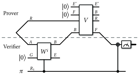
Figure 1: In quantum channel discrimination, the prover prepares a pure state $|\psi\rangle_{RA}$ and the verifier a mixed state $\pi:=\left(|0\rangle\langle 0|+|1\rangle\langle 1|\right)/2$. The verifier performs the controlled unitary in (11) that implements the conditional channel in (5). The prover acts on the channel output system $B$ and the reference system $R$ and sends back a single bit. The final controlled-NOT and computational basis measurement implement the measurement in (6).

The prover can optimize over all input states $\psi_{RA}$ and measurements $\{\Lambda_{RB}^{j}\}_{j\in\left\{0,1\right\}}$, and a well known result in quantum information [5] is that the optimal success probability of incoherent channel discrimination is given by

$$p_{s}^{\text{inc}}(\mathcal{N}^{0},\mathcal{N}^{1}) :=\sup_{\begin{subarray}{c}\psi_{RA},\\ \{\Lambda_{RB}^{j}\}_{j\in\left\{0,1\right\}}\end{subarray}}\frac{1}{2}\sum_{i\in\left\{0,1\right\}}\operatorname{Tr}[\Lambda_{RB}^{i}\mathcal{N}^{i}(\psi_{RA})]$$

$$=\frac{1}{2}\left(1+\frac{1}{2}\left\|\mathcal{N}^{0}-\mathcal{N}^{1}\right\|_{\diamond}\right),$$ (8)

thus endowing the normalized diamond distance $\frac{1}{2}\left\|\mathcal{N}^{0}-\mathcal{N}^{1}\right\|_{\diamond}$ with another operational meaning as the relative bias away from random guessing in a channel guessing game of the above form. That is, a random guessing strategy leads to a success probability of $1/2$ and can be employed when the channels are the same or indistinguishable. However, when the channels have some distinguishability so that $\frac{1}{2}\left\|\mathcal{N}^{0}-\mathcal{N}^{1}\right\|_{\diamond}\in(0,1]$, then the success probability changes as a linear function of the normalized diamond distance and reaches its peak value when the channels are orthogonal to each other (perfectly distinguishable). This guessing game is a basic channel discrimination task in quantum information theory and has found application in the setting of quantum illumination [7, 8, 13].

A useful fact about the diamond distance is that it can be computed by means of a semi-definite program [14]:

$$\frac{1}{2}\left\|\mathcal{N}^{0}-\mathcal{N}^{1}\right\|_{\diamond}=\inf_{\mu,Z_{RB}\geq 0}\left\{\begin{array}[c]{c}\mu:Z_{RB}\geq\Gamma_{RB}^{\mathcal{N}^{0}}-\Gamma_{RB}^{\mathcal{N}^{1}},\\ \mu I_{R}\geq\operatorname{Tr}_{B}[Z_{RB}]\end{array}\right\},$$ (9)

where $\Gamma_{RB}^{\mathcal{N}}:=\mathcal{N}_{A\rightarrow B}(\Gamma_{RA})$ is the Choi operator of the channel $\mathcal{N}_{A\rightarrow B}$, with $\Gamma_{RA}:=|\Gamma\rangle\langle\Gamma|_{RA}$ and $|\Gamma\rangle_{RA}:=\sum_{i}|i\rangle_{R}|i\rangle_{A}$, for orthonormal bases $\{|i\rangle_{R}\}_{i}$ and $\{|i\rangle_{A}\}_{i}$. Thus, calculating the diamond distance is efficient in the dimensions of the input $A$ and output $B$.

II Coherent Quantum Channel Discrimination

The main aim of the present paper is to introduce and analyze a fully quantum or coherent version of the channel guessing game presented above. Let us call it coherent quantum channel discrimination, in contrast to the incoherent channel discrimination task presented above. The primary modification that I make to it is to replace all classical steps of the verifier with their coherent counterparts, much like what was done previously in [15] to produce coherent versions of basic protocols in quantum information such as superdense coding and teleportation (see also [16] in this context). The resulting protocol is related to the fully quantum reading protocol from [17]. A recent series of works have considered coherent control of quantum channels [18, 19, 20, 21], but coherent quantum channel discrimination is different from the protocols considered in these prior works.

I now briefly summarize coherent channel discrimination. The main idea is to replace the initial state of the verifier with $|+\rangle_{R_{1}}:=\left(|0\rangle_{R_{1}}+|1\rangle_{R_{1}}\right)/\sqrt{2}$, the conditional channel of the verifier with a controlled unitary, and the final measurement with a projection onto the Bell state $|\Phi\rangle_{R_{1}F}:=\left(|00\rangle_{R_{1}F}+|11\rangle_{R_{1}F}\right)/\sqrt{2}$ (here and throughout the rest of the paper, we refer to both state vectors and density operators as states, as is conventional in the quantum information literature). Later, we shall see that it is sensible to include an uncomputing step to uncompute the controlled channel at the end before performing the Bell projection.

The modifications of the guessing game presented here could potentially have applications in quantum computation, where gates are often promoted to controlled gates and used in superposition. In particular, some works have recently investigated the question of compiling quantum circuits on quantum computers [22, 23]. The coherent games presented here could be used as benchmarks to assess how well an approximate implementation of a circuit could be used instead of the ideal one, even when it is employed in superposition (i.e., in controlled form). We do not investigate this particular application here but instead leave it for future work.

Before presenting details of the coherent version of the channel guessing game, let us recall some fundamental facts about quantum channels (see, e.g., [24]). First, every quantum channel $\mathcal{N}_{A\rightarrow B}$ has a Kraus representation as $\mathcal{N}_{A\rightarrow B}(\rho_{A})=\sum_{j}N^{j}\rho N^{j{\dagger}}$, where $\left\{N^{j}\right\}_{j}$ is a set of Kraus operators satisfying $\sum_{j}N^{j{\dagger}}N^{j}=I_{A}$. Another fundamental fact is that every quantum channel $\mathcal{N}_{A\rightarrow B}$ has an isometric extension. That is, to every quantum channel $\mathcal{N}_{A\rightarrow B}$, there exists an isometry $U_{A\rightarrow BE}$ (satisfying $U^{{\dagger}}U=I_{A}$) such that $\mathcal{N}_{A\rightarrow B}(\rho_{A})=\operatorname{Tr}_{E}[U_{A\rightarrow BE}(\rho_{A})(U_{A\rightarrow BE})^{{\dagger}}]$ for all input states $\rho_{A}$. Equivalently, there exists an environment system $G$ and a unitary $W_{AG\rightarrow BE}$ such that

$$\mathcal{N}_{A\rightarrow B}(\rho_{A})=\operatorname{Tr}_{E}[W_{AG\rightarrow BE}(\rho_{A}\otimes|0\rangle\langle 0|_{G})(W_{AG\rightarrow BE})^{{\dagger}}].$$ (10)

Thus, we can set $U_{A\rightarrow BE}=W_{AG\rightarrow BE}|0\rangle_{G}$. Any two isometric extensions of the original channel are related by an isometry acting on the environment system $E$.

The coherent version of the channel guessing game proceeds as follows. The verifier prepares the state $|+\rangle_{R_{1}}$ and the prover prepares $|\psi\rangle_{RA}$. The prover sends the system $A$ to the verifier. The verifier then adjoins the state $|0\rangle_{G}$ and performs the controlled unitary

$$\sum_{i\in\left\{0,1\right\}}|i\rangle\langle i|_{R_{1}}\otimes W_{AG\rightarrow BE}^{i},$$ (11)

where $W_{AG\rightarrow BE}^{i}$ is a unitary that extends the channel $\mathcal{N}_{A\rightarrow B}^{i}$ as in (10). Let $U_{A\rightarrow BE}^{i}:=W_{AG\rightarrow BE}^{i}|0\rangle_{G}$ be the corresponding isometric extension. The resulting state is then

$$\frac{1}{\sqrt{2}}\sum_{i\in\left\{0,1\right\}}|i\rangle_{R_{1}}W_{AG\rightarrow BE}^{i}|\psi\rangle_{RA}|0\rangle_{G}.$$ (12)

The verifier transmits system $B$ to the prover, who then adjoins an environment system $E^{\prime}$ in the state $|0\rangle_{E^{\prime}}$, a qubit system $F$ in the state $|0\rangle_{F}$, and performs a unitary $V_{RBE^{\prime}F}$. The resulting state is then

$$\frac{1}{\sqrt{2}}\sum_{i\in\left\{0,1\right\}}|i\rangle_{R_{1}}V_{RBE^{\prime}F}W_{AG\rightarrow BE}^{i}|\psi\rangle_{RA}|000\rangle_{GE^{\prime}F}.$$ (13)

The prover sends systems $B$ and $F$ back to the verifier, who uncomputes the controlled unitary in (11) by performing

$$\sum_{i\in\left\{0,1\right\}}|i\rangle\langle i|_{R_{1}}\otimes W_{AG\rightarrow BE}^{i{\dagger}}.$$ (14)

The state at this point is then

$$\frac{1}{\sqrt{2}}\sum_{i\in\left\{0,1\right\}}|i\rangle_{R_{1}}W^{i{\dagger}}VW^{i}|\psi\rangle_{RA}|000\rangle_{GE^{\prime}F},$$ (15)

where we omit system labels for brevity. The verifier finally performs the measurement

$$\left\{\Phi_{R_{1}F}\otimes|0\rangle\langle 0|_{G},I_{R_{1}FG}-\Phi_{R_{1}F}\otimes|0\rangle\langle 0|_{G}\right\}$$ (16)

on systems $R_{1}FG$, where $\Phi_{R_{1}F}\equiv|\Phi\rangle\langle\Phi|_{R_{1}F}$, and declares “success” (or “prover wins!”) if the first outcome occurs. The probability of success is equal to

$$p_{s}^{\text{coh}}(\mathcal{N}^{0},\mathcal{N}^{1},|\psi\rangle_{RA},V_{RBE^{\prime}F})\\ :=\frac{1}{2}\left\|\langle\Phi|_{R_{1}F}\langle 0|_{G}\sum_{i\in\left\{0,1\right\}}|i\rangle_{R_{1}}W^{i{\dagger}}VW^{i}|\psi\rangle_{RA}|000\rangle_{GE^{\prime}F}\right\|_{2}^{2}\\ =\frac{1}{2}\left\|\langle\Phi|_{R_{1}F}\sum_{i\in\left\{0,1\right\}}|i\rangle_{R_{1}}U^{i{\dagger}}VU^{i}|\psi\rangle_{RA}|00\rangle_{E^{\prime}F}\right\|_{2}^{2},$$ (17)

where the second expression follows from the fact that $U_{A\rightarrow BE}^{i}=W_{AG\rightarrow BE}^{i}|0\rangle_{G}$. Figure 2 depicts coherent quantum channel discrimination.

Figure 2: In coherent quantum channel discrimination, the prover prepares a pure state $|\psi\rangle_{RA}$ and the verifier the state $|+\rangle$. The verifier performs the controlled unitary in (11). The prover acts on the channel output system $B$ and reference system $R$ and sends $B$ back along with a single qubit. The verifier uncomputes the controlled unitary and finally implements the measurement in (16).

We can already observe that the success probability in (17) is independent of the particular isometric extension $U^{i}$ of the original channel $\mathcal{N}_{A\rightarrow B}^{i}$ for both $i=0$ and $i=1$. It is thus solely a function of the channels $\mathcal{N}_{A\rightarrow B}^{0}$ and $\mathcal{N}_{A\rightarrow B}^{1}$, as well as the particular strategy $\left\{|\psi\rangle_{RA},V_{RBE^{\prime}F}\right\}$ of the prover (as indicated by the notation in (17)). This follows because the unitary $V_{RBE^{\prime}F}$ that the prover performs does not act on the environment system $E$. Thus, letting $\widetilde{U}^{i}$ be some other isometric extension of $\mathcal{N}_{A\rightarrow B}^{i}$, it follows that $\widetilde{U}^{i{\dagger}}V\widetilde{U}^{i}=U^{i{\dagger}}VU^{i}$ by employing the previously stated fact that there exists an isometry $T_{E^{\prime}}$ (satisfying $T^{{\dagger}}T=I_{E^{\prime}}$) such that $\widetilde{U}^{i}=T_{E^{\prime}}U^{i}$.

Just as in the guessing game presented in Section I, the prover can optimize the success probability in (17) with respect to all possible strategies $\left\{|\psi\rangle_{RA},V_{RBE^{\prime}F}\right\}$. Let us denote the resulting success probability as follows:

$$p_{s}^{\text{coh}}(\mathcal{N}^{0},\mathcal{N}^{1}):=\sup_{|\psi\rangle,V}p_{s}^{\text{coh}}(\mathcal{N}^{0},\mathcal{N}^{1},|\psi\rangle_{RA},V_{RBE^{\prime}F}).$$ (18)

The main goal of this paper is to understand this quantity in more detail and relate it to the success probability in other forms of channel discrimination.

III Example

As a very simple example to demonstrate the task of coherent channel discrimination, suppose that the first channel $\mathcal{N}^{0}$ is the identity channel and the second $\mathcal{N}^{1}$ is the deterministic bit-flip channel, i.e., $\mathcal{N}^{1}(\cdot)=X(\cdot)X^{{\dagger}}$, where $X=\begin{bmatrix}0&1\\ 1&0\end{bmatrix}$ is the Pauli flip operator. These channels are orthogonal to each other, and a simple strategy for distinguishing them perfectly in incoherent channel discrimination is to input the state $|0\rangle$ and perform a computational basis measurement $\{|0\rangle\langle 0|,|1\rangle\langle 1|\}$. If the first channel is applied, the output state is $|0\rangle$, while if the second channel is applied, then the output state is $|1\rangle$, and these two states are perfectly distinguishable.

For coherent channel discrimination, the same input state is optimal. To see this, consider that the initial state of the verifier and prover’s systems is $|+\rangle_{R_{1}}|0\rangle_{A}$ (there is no reference system $R$ needed in this case). The controlled unitary in (11), implemented by the verifier, is then a controlled-NOT gate $|0\rangle\langle 0|\otimes I+|1\rangle\langle 1|\otimes X$, and there is no environment system $E$ because the channels are unitary channels. The resulting state after the controlled unitary is $|\Phi\rangle_{R_{1}B}$. The prover can then perform a controlled-NOT gate from system $B$ to system $F$, and the resulting state is a GHZ state: $(|000\rangle_{R_{1}BF}+|111\rangle_{R_{1}BF})/\sqrt{2}$. The verifier then performs the inverse of the controlled-NOT gate (itself a controlled-NOT), and the resulting state is $|\Phi\rangle_{R_{1}F}|0\rangle_{B}$, so that the Bell projection at the end succeeds with probability one; we thus arrive at the sensible conclusion that these channels are perfectly distinguishable in coherent channel discrimination.

This key example illustrates the necessity and sensibility of the uncomputing step in coherent channel discrimination. Without it, in this example, the final Bell projection would succeed only with probability $1/2$, leading to the unreasonable conclusion that these channels would not be perfectly distinguishable in coherent channel discrimination. Uncomputing is commonly employed in reversible and quantum computation as a “clean-up” step [25, 26, 27], and it serves the same purpose here.

IV Results

All proofs of the ensuing results appear in appendices.

IV-A Alternate expression

Proposition 1

For quantum channels $\mathcal{N}_{A\rightarrow B}^{0}$ and $\mathcal{N}_{A\rightarrow B}^{1}$, the success probability in (18) is equal to

$$p_{s}^{\text{coh}}(\mathcal{N}^{0},\mathcal{N}^{1})=\\ \left[\frac{1}{2}\sup_{\begin{subarray}{c}\left\{P^{i}\right\}_{i\in\left\{0,1\right\}}:\\ \sum_{i}P^{i{\dagger}}P^{i}=I_{RB}\end{subarray}}\left\|\sum_{i\in\left\{0,1\right\}}(\mathcal{N}_{A\rightarrow B}^{i})^{{\dagger}}(P_{RB\rightarrow RBE^{\prime}}^{i})\right\|_{\infty}\right]^{2}.$$ (19)

The operators $P_{RB\rightarrow RBE^{\prime}}^{i}$ act on the Hilbert space for $RB$ and take them to the Hilbert space for $RBE^{\prime}$. The dimension of $E^{\prime}$ need not be any larger than $2\left|A\right|\left|B\right|^{2}$.

In the above, the $\infty$-norm of an operator $X$ is defined as $\left\|X\right\|_{\infty}=\sup_{|\varphi\rangle\neq 0}\frac{\left\|X|\varphi\rangle\right\|_{2}}{\left\||\varphi\rangle\right\|_{2}}$ and the adjoint $\mathcal{N}^{{\dagger}}$ of a quantum channel $\mathcal{N}$ is defined to be the unique linear map satisfying $\operatorname{Tr}[[\mathcal{N}^{{\dagger}}(Y)]^{{\dagger}}X]=\operatorname{Tr}[Y^{{\dagger}}\mathcal{N}(X)]$ for all operators $X$ and $Y$.

It is interesting to contrast the expression in (19) with the following expression for the success probability of incoherent channel discrimination:

$$p_{s}^{\text{inc}}(\mathcal{N}^{0},\mathcal{N}^{1})=\frac{1}{2}\sup_{\left\{\Lambda_{RB}^{i}\right\}_{i\in\left\{0,1\right\}}}\left\|\sum_{i\in\left\{0,1\right\}}(\mathcal{N}_{A\rightarrow B}^{i})^{{\dagger}}(\Lambda_{RB}^{i})\right\|_{\infty},$$ (20)

where $\sum_{i\in\left\{0,1\right\}}\Lambda_{RB}^{i}=I_{RB}$ and $\Lambda_{RB}^{i}\geq 0$. This expression comes about from that in (8) by employing the definition of the $\infty$-norm and the adjoint of a quantum channel. Even by examining these expressions, we can see how (19) is a coherent version of (20). The expression in (19) is like the square of a probability amplitude (the latter being the expression inside the $\infty$-norm), and it involves operators for which the sum of their squares is equal to the identity instead of their sums being equal to the identity.

IV-B Bounds on success probability

Proposition 2

The following bounds hold for the success probability in (18):

$$1/2\leq p_{s}^{\text{coh}}(\mathcal{N}^{0},\mathcal{N}^{1})\leq 1.$$ (21)

The upper bound is saturated if and only if the channels are orthogonal (i.e., there exists a pure state $\psi_{RA}$ such that $\mathcal{N}_{A\rightarrow B}^{0}(\psi_{RA})\mathcal{N}_{A\rightarrow B}^{1}(\psi_{RA})=0$). The lower bound is saturated if the channels are identical (i.e., indistinguishable).

The upper bound is obvious since $p_{s}^{\text{coh}}$ is a probability, and the necessary and sufficient condition for saturation follows by employing the bounds

$$p_{s}^{\text{coh}}(\mathcal{N}^{0},\mathcal{N}^{1})\leq p_{s}^{\text{inc}}(\mathcal{N}^{0},\mathcal{N}^{1})\leq\sqrt{p_{s}^{\text{coh}}(\mathcal{N}^{0},\mathcal{N}^{1})},$$ (22)

discussed later. The lower bound follows by setting $P^{i}=\sqrt{1/2}I_{RB}\otimes|0\rangle_{E^{\prime}}$ for $i\in\left\{0,1\right\}$ in (19), which corresponds to “not even trying to distinguish,” and the sufficient saturation condition follows by direct evaluation.

IV-C Non-increase under a superchannel

A key property of the success probability $p_{s}^{\text{coh}}(\mathcal{N}^{0},\mathcal{N}^{1})$ in (18) is that it does not increase under the action of a quantum superchannel. This is a basic property expected of any channel distinguishability measure, and it was recently shown that the diamond distance (and thus the success probability in (8)) satisfies this property [28].

To expand upon this statement, recall from [29] that a quantum superchannel is a physical mapping of a quantum channel to a quantum channel, and it should be this way even when acting on one share of an arbitrary bipartite channel. In more detail, a superchannel $\Theta_{\left(A\rightarrow B\right)\rightarrow(C\rightarrow D)}$ is a linear map that completely preserves the properties of complete positivity and trace preservation. Then for an arbitrary input bipartite channel $\mathcal{M}_{RA\rightarrow RB}$, the output $\Theta_{\left(A\rightarrow B\right)\rightarrow(C\rightarrow D)}(\mathcal{M}_{RA\rightarrow RB})$ is a bipartite channel from systems $RC$ to systems $RD$. The fundamental theorem of superchannels is that any superchannel has a physical realization in terms of a pre-processing channel $\mathcal{E}_{C\rightarrow AM}$ and a post-processing channel $\mathcal{D}_{BM\rightarrow D}$ [29]:

$$\Theta_{\left(A\rightarrow B\right)\rightarrow(C\rightarrow D)}(\mathcal{M}_{RA\rightarrow RB})=\\ \mathcal{D}_{BM\rightarrow D}\circ\mathcal{M}_{RA\rightarrow RB}\circ\mathcal{E}_{C\rightarrow AM}.$$ (23)

With the fundamental theorem of superchannels in hand, we can arrive at an operational proof that the success probability in (18) does not increase under the action of a superchannel. To see this, consider that a particular strategy of the prover for coherently distinguishing the channels $\mathcal{N}^{0}$ and $\mathcal{N}^{1}$ is to prepare a state $|\psi\rangle_{RC}$ and act with an isometric extension $U_{C\rightarrow AMM_{1}}^{\mathcal{E}}$ of the pre-processing $\mathcal{E}_{C\rightarrow AM}$ on system $C$. Then the verifier performs the controlled unitary in (11), and the prover performs an isometric extension $U_{BM\rightarrow DM_{2}}^{\mathcal{D}}$ of the post-processing $\mathcal{D}_{BM\rightarrow D}$, the unitary $V_{RBE^{\prime}F}$, and the adjoint of $U_{BM\rightarrow DM_{2}}^{\mathcal{D}}$ (the last being implemented by a unitary and a projection). The verifier finally performs the inverse of (11) and the projective measurement in (16). Since the success probability does not increase under the action of the adjoint of $U_{C\rightarrow AMM_{1}}^{\mathcal{E}}$ and since this is a particular strategy for coherent discrimination of $\mathcal{N}^{0}$ and $\mathcal{N}^{1}$, while being a general strategy for coherent discrimination of $\Theta(\mathcal{N}^{0})$ and $\Theta(\mathcal{N}^{1})$, we conclude that the success probability does not increase under the action of a superchannel:

Theorem 1

Let $\mathcal{N}_{A\rightarrow B}^{0}$ and $\mathcal{N}_{A\rightarrow B}^{1}$ be quantum channels, and let $\Theta_{\left(A\rightarrow B\right)\rightarrow(C\rightarrow D)}$ be a quantum superchannel. Then the success probability of coherent channel discrimination in (18) does not increase under the action of $\Theta_{\left(A\rightarrow B\right)\rightarrow(C\rightarrow D)}$:

$$p_{s}^{\text{coh}}(\mathcal{N}^{0},\mathcal{N}^{1})\geq p_{s}^{\text{coh}}(\Theta(\mathcal{N}^{0}),\Theta(\mathcal{N}^{1})).$$ (24)

A strictly mathematical proof of (24) is to employ (19), the fundamental theorem of superchannels in (23), and the fact that the $\infty$-norm does not increase under the action of a completely positive unital map or a projection.

IV-D Computable by semi-definite programming

The success probability in (18) can be computed by means of the following semi-definite program:

$$\sup_{\begin{subarray}{c}\sigma_{R_{1}FBE},\\ \rho_{A}\end{subarray}}\left\{\operatorname{Tr}[Y_{R_{1}FBE}\sigma_{R_{1}FBE}]:\operatorname{Tr}_{BF}[\sigma_{R_{1}FBE}]=Z_{R_{1}E}^{\rho}\right\},$$ (25)

where $\sigma_{R_{1}FBE}$ and $\rho_{A}$ are density operators and

$$Y_{R_{1}FBE} :=\frac{1}{2}\sum_{i,j\in\left\{0,1\right\},k,\ell}|ii\rangle\langle jj|_{R_{1}F}\otimes N_{k}^{i}N_{\ell}^{j{\dagger}}\otimes|k\rangle\langle\ell|_{E},$$

$$Z_{R_{1}E}^{\rho} :=\frac{1}{2}\sum_{i,j\in\left\{0,1\right\},k,\ell}\operatorname{Tr}[N_{\ell}^{j{\dagger}}N_{k}^{i}\rho_{A}]|i\rangle\langle j|_{R_{1}}\otimes|k\rangle\langle\ell|_{E},$$

with $\{N_{k}^{i}\}_{k}$ a set of Kraus operators for the channel $\mathcal{N}_{A\rightarrow B}^{i}$ for $i\in\left\{0,1\right\}$. This follows from the observation that coherent channel discrimination is a quantum interactive proof, and the acceptance probability of any quantum interactive proof can be calculated by means of a semi-definite program [30, 10]. In the above semi-definite program, the density operator $\rho_{A}$ can be understood as the reduction of the initial state of the prover on system $A$, and the density operator $Z_{R_{1}E}^{\rho}$ is the reduced state from (12) on systems $R_{1}E$. The projection $Y_{R_{1}FBE}$ corresponds to the concatenation of the inverse unitary in (14) followed by the projection in (16) onto the accepting subspace. The equality constraint in (25) corresponds to the fact that the state of the verifier on systems $R_{1}$ and $E$ should be the same before and after the prover acts with the unitary $V_{RBE^{\prime}F}$.

The dual semi-definite program is given by

$$\inf_{\lambda,W_{R_{1}E}}\lambda$$ subject to (26)

$$W_{R_{1}E}\otimes I_{BF} \geq Y_{R_{1}EBF},$$ (27)

$$\lambda I_{A} \geq\frac{1}{2}\sum_{i,j\in\left\{0,1\right\},k,\ell}w_{R_{1}E}^{ikj\ell}N_{k}^{i{\dagger}}N_{\ell}^{j},$$ (28)

where $\lambda\in\mathbb{R}$, the operator $W_{R_{1}E}$ is Hermitian, and $w_{R_{1}E}^{ikj\ell}:=\langle i|_{R_{1}}\langle k|_{E}W_{R_{1}E}|j\rangle_{R_{1}}|\ell\rangle_{E}$. This follows by the standard Lagrange multiplier method.

V Incoherent Channel Discrimination with Uncomputing

Another variation of channel discrimination is to follow the same protocol for coherent channel discrimination but have the initial state be the maximally mixed state and the final measurement be as in (6), with the first outcome indicating success. So this is the main difference with coherent channel discrimination, and the main difference with incoherent channel discrimination is that we include a step for uncomputing. Let $p_{s}^{\text{inc,unc}}(\mathcal{N}^{0},\mathcal{N}^{1})$ denote the success probability for this case. We then have the following bounds, implying (22):

$$p_{s}^{\text{coh}}\leq p_{s}^{\text{inc,unc}}\leq p_{s}^{\text{inc}}\leq\sqrt{p_{s}^{\text{coh}}},$$ (29)

where the channel arguments are left implicit for brevity.

VI Conclusion

This paper has introduced a coherent version of quantum channel discrimination and investigated various aspects of the success probability. I have proven an alternate expression for it in Proposition 1, some bounds in Proposition 2 and Eq. (29), that it does not increase under the action of a quantum superchannel, and that it can be calculated by means of a semi-definite program. An intriguing open question is to determine if $p_{s}^{\text{coh}}-1/2$ is a metric on quantum channels. Consider that $p_{s}^{\text{inc}}-1/2$ is, as is clear from (8).

Appendix A Proof of Proposition 1

Let us begin with the expression in (17) for the unoptimized success probability:

$$\frac{1}{2}\left\|\langle\Phi|_{R_{1}F}\sum_{i\in\left\{0,1\right\}}|i\rangle_{R_{1}}U^{i{\dagger}}VU^{i}|\psi\rangle_{RA}|00\rangle_{E^{\prime}F}\right\|_{2}^{2}$$

$$=\frac{1}{4}\left\|\sum_{i,j\in\left\{0,1\right\}}\langle jj|_{R_{1}F}|i\rangle_{R_{1}}U^{i{\dagger}}VU^{i}|\psi\rangle_{RA}|00\rangle_{E^{\prime}F}\right\|_{2}^{2}$$ (30)

$$=\frac{1}{4}\left\|\sum_{i\in\left\{0,1\right\}}\langle i|_{F}U^{i{\dagger}}VU^{i}|\psi\rangle_{RA}|00\rangle_{E^{\prime}F}\right\|_{2}^{2}$$ (31)

$$=\frac{1}{4}\left\|\sum_{i\in\left\{0,1\right\}}\langle i|_{F}\mathcal{N}^{i{\dagger}}(V)|\psi\rangle_{RA}|00\rangle_{E^{\prime}F}\right\|_{2}^{2},$$ (32)

where we used the fact that $U^{i{\dagger}}VU^{i}$ can be expressed in terms of the channel adjoint as $\mathcal{N}^{i{\dagger}}(V)$ [24]. Let us write

$$V_{RBE^{\prime}F}=\sum_{j,k\in\left\{0,1\right\}}Q_{RBE^{\prime}}^{j,k}\otimes|j\rangle\langle k|_{F},$$ (33)

where the operators $Q_{RBE^{\prime}}^{j,k}$ satisfy

$$Q_{RBE^{\prime}}^{0,0{\dagger}}Q_{RBE^{\prime}}^{0,0}+Q_{RBE^{\prime}}^{1,0{\dagger}}Q_{RBE^{\prime}}^{1,0} =I_{RBE^{\prime}},$$ (34)

$$Q_{RBE^{\prime}}^{0,1{\dagger}}Q_{RBE^{\prime}}^{0,0}+Q_{RBE^{\prime}}^{1,1{\dagger}}Q_{RBE^{\prime}}^{1,0} =0,$$ (35)

$$Q_{RBE^{\prime}}^{0,0{\dagger}}Q_{RBE^{\prime}}^{0,1}+Q_{RBE^{\prime}}^{1,0{\dagger}}Q_{RBE^{\prime}}^{1,1} =0,$$ (36)

$$Q_{RBE^{\prime}}^{0,1{\dagger}}Q_{RBE^{\prime}}^{0,1}+Q_{RBE^{\prime}}^{1,1{\dagger}}Q_{RBE^{\prime}}^{1,1} =I_{RBE^{\prime}},$$ (37)

in order for $V_{RBE^{\prime}F}$ to be unitary. Then we find that

$$\langle i|_{F}\mathcal{N}^{i{\dagger}}(V)|\psi\rangle_{RA}|00\rangle_{E^{\prime}F}$$

$$=\sum_{j,k\in\left\{0,1\right\}}\langle i|_{F}\left[\mathcal{N}^{i{\dagger}}(Q_{RBE^{\prime}}^{j,k})\otimes|j\rangle\langle k|_{F}\right]|\psi\rangle_{RA}|00\rangle_{E^{\prime}F}$$

$$=\mathcal{N}^{i{\dagger}}(Q_{RBE^{\prime}}^{i,0})|\psi\rangle_{RA}|0\rangle_{E^{\prime}}$$

$$=\mathcal{N}^{i{\dagger}}(Q_{RBE^{\prime}}^{i,0}|0\rangle_{E^{\prime}})|\psi\rangle_{RA}$$ (38)

which leads to

$$\text{Eq.}~{}\eqref{eq:pf-simpler-exp-1}=\frac{1}{4}\left\|\sum_{i\in\left\{0,1\right\}}\mathcal{N}^{i{\dagger}}(Q_{RBE^{\prime}}^{i,0}|0\rangle_{E^{\prime}})|\psi\rangle_{RA}\right\|_{2}^{2}.$$ (39)

Now optimizing over all input states $|\psi\rangle_{RA}$ and unitaries $V_{RBE^{\prime}F}$, while setting

$$P_{RB\rightarrow RBE^{\prime}}^{i}:=Q_{RBE^{\prime}}^{i,0}|0\rangle_{E^{\prime}},$$ (40)

we find that

$$p_{s}^{\text{coh}}(\mathcal{N}^{0},\mathcal{N}^{1})=\\ \sup_{{}_{\begin{subarray}{c}\left\{P^{i}\right\}_{i\in\left\{0,1\right\}}:\\ \sum_{i}P^{i{\dagger}}P^{i}=I_{RB}\end{subarray}}}\frac{1}{4}\left\|\sum_{i\in\left\{0,1\right\}}\mathcal{N}^{i{\dagger}}(P_{RB\rightarrow RBE^{\prime}}^{i})\right\|_{\infty}^{2}.$$ (41)

Also, note that to any set $\left\{P^{i}\right\}_{i\in\left\{0,1\right\}}$ satisfying $\sum_{i}P^{i{\dagger}}P^{i}=I_{RB}$, we can complete it to a unitary $V_{RBE^{\prime}F}$.

Since the unitary $V_{RBE^{\prime}F}$ implements a quantum channel from systems $RB$ to $BF$, and since the dimension of the environment of any quantum channel need not be larger than the product of the input and output dimensions, it suffices to take $\left|E^{\prime}\right|=\left|R\right|\left|B\right|^{2}\left|F\right|$. Since $\left|R\right|=\left|A\right|$ and $\left|F\right|=2$, it suffices to take $\left|E^{\prime}\right|=2\left|A\right|\left|B\right|^{2}$ as claimed.

Appendix B Proof of Proposition 2

The upper bound in (21) trivially follows because $p_{s}^{\text{coh}}(\mathcal{N}^{0},\mathcal{N}^{1})$ is a probability. The lower bound in (21) follows by picking $P_{RB\rightarrow RBE^{\prime}}^{i}=\sqrt{1/2}I_{RB}\otimes|0\rangle_{E^{\prime}}$ for $i\in\left\{0,1\right\}$ and evaluating (19). Consider that

$$\left[\frac{1}{2}\sup_{\begin{subarray}{c}\left\{P^{i}\right\}_{i\in\left\{0,1\right\}}:\\ \sum_{i}P^{i{\dagger}}P^{i}=I_{RB}\end{subarray}}\left\|\sum_{i\in\left\{0,1\right\}}(\mathcal{N}_{A\rightarrow B}^{i})^{{\dagger}}(P_{RB\rightarrow RBE^{\prime}}^{i})\right\|_{\infty}\right]^{2}$$

$$\geq\left[\frac{1}{2}\left\|\sqrt{\frac{1}{2}}\sum_{i\in\left\{0,1\right\}}(\mathcal{N}_{A\rightarrow B}^{i})^{{\dagger}}(I_{RB}\otimes|0\rangle_{E^{\prime}})\right\|_{\infty}\right]^{2}$$ (42)

$$=\left[\frac{1}{2\sqrt{2}}\left\|2(I_{RB}\otimes|0\rangle_{E^{\prime}})\right\|_{\infty}\right]^{2}$$ (43)

$$=\left[\frac{1}{\sqrt{2}}\right]^{2}=\frac{1}{2}.$$ (44)

The first inequality follows by picking $P_{RB\rightarrow RBE^{\prime}}^{i}$ as indicated. The first equality follows because $(\mathcal{N}_{A\rightarrow B}^{i})^{{\dagger}}$ is a unital map.

If the channels $\mathcal{N}_{A\rightarrow B}^{0}$ and $\mathcal{N}_{A\rightarrow B}^{1}$ are the same (so that $\mathcal{N}_{A\rightarrow B}^{0}=\mathcal{N}_{A\rightarrow B}^{1}=\mathcal{N}_{A\rightarrow B}$), then consider for $\left\{P^{i}\right\}_{i\in\left\{0,1\right\}}$ satisfying $\sum_{i\in\left\{0,1\right\}}P^{i{\dagger}}P^{i}=I_{RB}$ that

$$\left[\frac{1}{2}\left\|\sum_{i\in\left\{0,1\right\}}(\mathcal{N}_{A\rightarrow B}^{i})^{{\dagger}}(P_{RB\rightarrow RBE^{\prime}}^{i})\right\|_{\infty}\right]^{2}$$

$$=\left[\frac{1}{2}\left\|(\mathcal{N}_{A\rightarrow B})^{{\dagger}}\left(\sum_{i\in\left\{0,1\right\}}P_{RB\rightarrow RBE^{\prime}}^{i}\right)\right\|_{\infty}\right]^{2}$$ (45)

$$\leq\left[\frac{1}{2}\left\|\sum_{i\in\left\{0,1\right\}}P_{RB\rightarrow RBE^{\prime}}^{i}\right\|_{\infty}\right]^{2}$$ (46)

$$=\frac{1}{4}\left\|\sum_{i\in\left\{0,1\right\}}P_{RB\rightarrow RBE^{\prime}}^{i}\right\|_{\infty}^{2}$$ (47)

$$=\frac{1}{4}\left\|\left(\sum_{j\in\left\{0,1\right\}}P_{RB\rightarrow RBE^{\prime}}^{j{\dagger}}\right)\left(\sum_{i\in\left\{0,1\right\}}P_{RB\rightarrow RBE^{\prime}}^{i}\right)\right\|_{\infty}$$ (48)

$$=\frac{1}{4}\left\|P^{0{\dagger}}P^{0}+P^{1{\dagger}}P^{1}+P^{1{\dagger}}P^{0}+P^{0{\dagger}}P^{1}\right\|_{\infty}$$ (49)

$$\leq\frac{1}{4}\left\|2\left(P^{0{\dagger}}P^{0}+P^{1{\dagger}}P^{1}\right)\right\|_{\infty}$$ (50)

$$=1/2.$$ (51)

The first equality follows from the assumption that the channels are the same. The first inequality follows because the operator norm is non-increasing under the action of a completely positive unital map [31]. The third equality follows because $\left\|A\right\|_{\infty}^{2}=\left\|A^{{\dagger}}A\right\|_{\infty}$. The second inequality follows because

$$P^{1{\dagger}}P^{0}+P^{0{\dagger}}P^{1}\leq P^{0{\dagger}}P^{0}+P^{1{\dagger}}P^{1},$$ (52)

which is equivalent to

$$\left(P^{0{\dagger}}-P^{1{\dagger}}\right)\left(P^{0}-P^{1}\right)\geq 0.$$ (53)

The final equality follows because $\sum_{i\in\left\{0,1\right\}}P^{i{\dagger}}P^{i}=I_{RB}$ and $\left\|I\right\|_{\infty}=1$. Since the lower bound in (21) always holds, we conclude that $p_{s}^{\text{coh}}(\mathcal{N}^{0},\mathcal{N}^{1})=1/2$ if $\mathcal{N}^{0}=\mathcal{N}^{1}$.

If the channels $\mathcal{N}^{0}$ and $\mathcal{N}^{1}$ are perfectly distinguishable, then this means that $p_{s}^{\text{inc}}(\mathcal{N}^{0},\mathcal{N}^{1})=1$. Applying the upper bound in (22) implies that $p_{s}^{\text{coh}}(\mathcal{N}^{0},\mathcal{N}^{1})=1$. If instead $p_{s}^{\text{coh}}(\mathcal{N}^{0},\mathcal{N}^{1})=1$, then the lower bound in (22) implies that $p_{s}^{\text{inc}}(\mathcal{N}^{0},\mathcal{N}^{1})=1$. Then if $p_{s}^{\text{inc}}(\mathcal{N}^{0},\mathcal{N}^{1})=1$, it is known that $\mathcal{N}^{0}$ and $\mathcal{N}^{1}$ are perfectly distinguishable. The bounds in (22) are proved in Appendix E.

Appendix C Proof of Theorem 1

This appendix establishes a proof of Theorem 1, which states that the success probability in (18) does not increase under the action of a quantum superchannel.

First let us consider a more mathematical proof that requires fewer steps. Let $\Theta_{\left(A\rightarrow B\right)\rightarrow\left(C\rightarrow D\right)}$ denote a quantum superchannel. Exploiting the expression in (19), we can write the success probability $p_{s}^{\text{coh}}(\Theta(\mathcal{N}^{0}),\Theta(\mathcal{N}^{1}))$ as

$$p_{s}^{\text{coh}}(\Theta(\mathcal{N}^{0}),\Theta(\mathcal{N}^{1}))=\\ \left[\frac{1}{2}\sup_{\begin{subarray}{c}\left\{Q^{i}\right\}_{i}:\\ \sum_{i}Q^{i{\dagger}}Q^{i}=I\end{subarray}}\left\|\sum_{i\in\left\{0,1\right\}}(\Theta(\mathcal{N}_{A\rightarrow B}^{i}))^{{\dagger}}(Q_{RD\rightarrow RDE^{\prime\prime}}^{i})\right\|_{\infty}\right]^{2}.$$ (54)

Let $\left\{Q^{i}\right\}_{i\in\left\{0,1\right\}}$ be an arbitrary set of operators satisfying $\sum_{i}Q^{i{\dagger}}Q^{i}=I_{RD}$. Then consider from the fundamental theorem of superchannels in (23) that

$$\left\|\sum_{i\in\left\{0,1\right\}}(\Theta(\mathcal{N}_{A\rightarrow B}^{i}))^{{\dagger}}(Q_{RD\rightarrow RDE^{\prime\prime}}^{i})\right\|_{\infty}$$

$$=\left\|\sum_{i\in\left\{0,1\right\}}((\mathcal{E}_{C\rightarrow AM})^{{\dagger}}\circ(\mathcal{N}_{A\rightarrow B}^{i})^{{\dagger}}\circ(\mathcal{D}_{BM\rightarrow D})^{{\dagger}})(Q^{i})\right\|_{\infty}$$

$$\leq\left\|\sum_{i\in\left\{0,1\right\}}((\mathcal{N}_{A\rightarrow B}^{i})^{{\dagger}}\circ(\mathcal{D}_{BM\rightarrow D})^{{\dagger}})(Q_{RD\rightarrow RDE^{\prime\prime}}^{i})\right\|_{\infty},$$ (55)

where the inequality follows from the fact that a completely positive unital map does not increase the operator norm [31]. Let $W_{BMG^{\prime}\rightarrow DM_{2}}$ be a unitary extension of $\mathcal{D}_{BM\rightarrow D}$, with input environment $G^{\prime}$ and output environment $M_{2}$, so that

$$\mathcal{D}_{BM\rightarrow D}(\cdot)=\\ \operatorname{Tr}_{M_{2}}[W_{BMG^{\prime}\rightarrow DM_{2}}[(\cdot)\otimes|0\rangle\langle 0|_{G^{\prime}}](W_{BMG^{\prime}\rightarrow DM_{2}})^{{\dagger}}].$$ (56)

Then it is well known [24] that

$$(\mathcal{D}_{BM\rightarrow D})^{{\dagger}}(\cdot)=\\ \langle 0|_{G^{\prime}}(W_{BMG^{\prime}\rightarrow DM_{2}})^{{\dagger}}[(\cdot)\otimes I_{M_{2}}]W_{BMG^{\prime}\rightarrow DM_{2}}|0\rangle_{G^{\prime}}.$$ (57)

Substituting above, we find that

$$\text{Eq.}~{}\eqref{eq:superch-mathy-1}$$

$$=\left\|\sum_{i\in\left\{0,1\right\}}(\mathcal{N}_{A\rightarrow B}^{i})^{{\dagger}}(\langle 0|_{G^{\prime}}W^{{\dagger}}(Q^{i}\otimes I_{M^{\prime}})W|0\rangle_{G^{\prime}})\right\|_{\infty}$$

$$\leq\left\|\sum_{i\in\left\{0,1\right\}}(\mathcal{N}_{A\rightarrow B}^{i})^{{\dagger}}(W^{{\dagger}}(Q_{RD\rightarrow RDE^{\prime\prime}}^{i}\otimes I_{M^{\prime}})W|0\rangle_{G^{\prime}})\right\|_{\infty}$$

$$\leq\sup_{\begin{subarray}{c}\left\{P^{i}\right\}_{i\in\left\{0,1\right\}}:\\ \sum_{i}P^{i{\dagger}}P^{i}=I_{RB}\end{subarray}}\left\|\sum_{i\in\left\{0,1\right\}}(\mathcal{N}_{A\rightarrow B}^{i})^{{\dagger}}(P_{RB\rightarrow RBE^{\prime}}^{i})\right\|_{\infty}$$

$$=2\sqrt{p_{s}^{\text{coh}}(\mathcal{N}^{0},\mathcal{N}^{1})}.$$ (58)

The first inequality follows because a projection onto $\langle 0|_{G^{\prime}}$ does not increase the operator norm, and the second inequality follows because the set $\{W^{{\dagger}}(Q_{RD\rightarrow RDE^{\prime\prime}}^{i}\otimes I_{M^{\prime}})W|0\rangle_{G^{\prime}}\}_{i}$ is a particular choice of $\left\{P^{i}\right\}_{i\in\left\{0,1\right\}}$ satisfying $\sum_{i}P^{i{\dagger}}P^{i}=I_{RB}$. We then conclude the inequality in (24) since $\left\{Q^{i}\right\}_{i\in\left\{0,1\right\}}$ is an arbitrary set of operators satisfying $\sum_{i}Q^{i{\dagger}}Q^{i}=I_{RD}$.

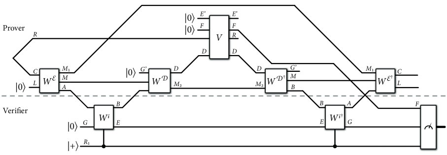
Figure 3: Depiction of the operational proof of Theorem 1. This is a particular strategy for coherent channel discrimination of the channels $\mathcal{N}_{A\rightarrow B}^{0}$ and $\mathcal{N}_{A\rightarrow B}^{1}$, but it is a general strategy for coherent channel discrimination of $\Theta(\mathcal{N}_{A\rightarrow B}^{0})$ and $\Theta(\mathcal{N}_{A\rightarrow B}^{1})$, where $\Theta_{\left(A\rightarrow B\right)\rightarrow\left(C\rightarrow D\right)}$ is a quantum superchannel.

A more operational proof of Theorem 1 goes along the lines discussed in Section IV-C and is depicted in Figure 3. The main idea behind this operational proof is that the strategy depicted in Figure 3 is a particular strategy for coherent channel discrimination of the channels $\mathcal{N}_{A\rightarrow B}^{0}$ and $\mathcal{N}_{A\rightarrow B}^{1}$, but it is a general strategy for coherent channel discrimination of the channels $\Theta(\mathcal{N}_{A\rightarrow B}^{0})$ and $\Theta(\mathcal{N}_{A\rightarrow B}^{1})$, where $\Theta_{\left(A\rightarrow B\right)\rightarrow\left(C\rightarrow D\right)}$ is a quantum superchannel. Let $W_{AG\rightarrow BE}^{i}$ be a unitary extension of the channel $\mathcal{N}_{A\rightarrow B}^{i}$, so that

$$\mathcal{N}_{A\rightarrow B}^{i}(\cdot)=\\ \operatorname{Tr}_{E}[W_{AG\rightarrow BE}^{i}((\cdot)\otimes|0\rangle\langle 0|_{E})(W_{AG\rightarrow BE}^{i})^{{\dagger}}].$$ (59)

Let $\Theta_{\left(A\rightarrow B\right)\rightarrow\left(C\rightarrow D\right)}$ be a quantum superchannel, and by the fundamental theorem of superchannels, it has a physical realization as in (23). Let $W_{CL\rightarrow AMM_{1}}^{\mathcal{E}}$ be a unitary extension of the channel $\mathcal{E}_{A\rightarrow BM}$, and let $W_{BMG^{\prime}\rightarrow DM_{2}}^{\mathcal{D}}$ be a unitary extension of the channel $\mathcal{D}_{BM\rightarrow D}$, so that

$$\mathcal{E}_{A\rightarrow BM}(\cdot)=\\ \operatorname{Tr}_{M_{1}}[W_{CL\rightarrow AMM_{1}}^{\mathcal{E}}((\cdot)\otimes|0\rangle\langle 0|_{L})(W_{CL\rightarrow AMM_{1}}^{\mathcal{E}})^{{\dagger}}].$$ (60)

and

$$\mathcal{D}_{BM\rightarrow D}(\cdot)=\\ \operatorname{Tr}_{M_{2}}[W_{BMG^{\prime}\rightarrow DM_{2}}^{\mathcal{D}}((\cdot)\otimes|0\rangle\langle 0|_{G^{\prime}})(W_{BMG^{\prime}\rightarrow DM_{2}}^{\mathcal{D}})^{{\dagger}}].$$ (61)

From (32), we know that the success probability for coherent channel discrimination of $\Theta(\mathcal{N}_{A\rightarrow B}^{0})$ and $\Theta(\mathcal{N}_{A\rightarrow B}^{1})$, for a fixed strategy $\left\{|\psi\rangle_{RC},V_{RDFE^{\prime}}\right\}$, is given by

$$\frac{1}{4}\left\|\sum_{i\in\left\{0,1\right\}}\langle i|_{F}T^{i{\dagger}}VT^{i}|\psi\rangle_{RC}|00\rangle_{E^{\prime}F}\right\|_{2}^{2},$$ (62)

where for $i\in\left\{0,1\right\}$,

$$T_{C\rightarrow DM_{1}M_{2}E}^{i}:=\\ W_{BMG^{\prime}\rightarrow DM_{2}}^{\mathcal{D}}W_{AG\rightarrow BE}^{i}W_{CL\rightarrow AMM_{1}}^{\mathcal{E}}|0\rangle_{L}|0\rangle_{G}|0\rangle_{G^{\prime}}.$$ (63)

This follows because $T_{C\rightarrow DM_{1}M_{2}E}^{i}$ is an isometric extension of the channel $\Theta(\mathcal{N}_{A\rightarrow B}^{i})$ for $i\in\left\{0,1\right\}$. Since the Euclidean norm is non-increasing with respect to the projections onto $|0\rangle_{L}$ and $|0\rangle_{G^{\prime}}$, we find that

Eq. (62)

$$\leq\frac{1}{4}\left\|\sum_{i\in\left\{0,1\right\}}\langle i|_{F}\langle 0|_{G}W^{\mathcal{E{\dagger}}}W^{i{\dagger}}W^{\mathcal{D{\dagger}}}VT^{i}|\psi\rangle_{RC}|00\rangle_{E^{\prime}F}\right\|_{2}^{2}$$

$$=\frac{1}{4}\left\|\sum_{i\in\left\{0,1\right\}}\langle i|_{F}\langle 0|_{G}W^{i{\dagger}}W^{\mathcal{D{\dagger}}}VT^{i}|\psi\rangle_{RC}|00\rangle_{E^{\prime}F}\right\|_{2}^{2},$$ (64)

where for the last equality we used that $W_{CL\rightarrow AMM_{1}}^{\mathcal{E}}$ is unitary and not acting on any of the systems being projected out. Now we observe that $W_{CL\rightarrow AMM_{1}}^{\mathcal{E}}|\psi\rangle_{RC}|0\rangle_{L}|0\rangle_{G^{\prime}}$ is a particular pure state that the prover can use for coherent channel discrimination of $\mathcal{N}_{A\rightarrow B}^{0}$ and $\mathcal{N}_{A\rightarrow B}^{1}$, and $(W_{BMG^{\prime}\rightarrow DM_{2}}^{\mathcal{D}})^{{\dagger}}V_{RDFE^{\prime}}W_{BMG^{\prime}\rightarrow DM_{2}}^{\mathcal{D}}$ is a particular unitary that the prover can use for the same purpose. So we conclude that

$$\text{Eq.}~{}\eqref{eq:super-ch-proof-oper-final}\leq p_{s}^{\text{coh}}(\mathcal{N}^{0},\mathcal{N}^{1}).$$ (65)

Since the strategy employed for distinguishing $\Theta(\mathcal{N}_{A\rightarrow B}^{0})$ and $\Theta(\mathcal{N}_{A\rightarrow B}^{1})$ is arbitrary, we conclude the operational proof of Theorem 1.

Appendix D Proof of Semi-definite programming formulation in Eq. (25)

Here I establish the particular form of the success probability in (25), which demonstrates that (18) can be calculated by means of a semi-definite program. As stated previously, this follows from the fact that coherent channel discrimination is a quantum interactive proof system, and the acceptance probability of any quantum interactive proof system can be calculated via a semi-definite program [30, 10]. In particular, coherent channel discrimination is a three-message quantum interactive proof system. Recall from [10, Section 4.3] that a three-message interactive proof system is specified by two linear isometries $T_{Y_{0}\rightarrow Z_{1}X_{1}}^{1}$ and $T_{Z_{1}Y_{1}\rightarrow Z_{2}}^{2}$ for the initial circuit of the verifier and the final circuit of the verifier before the measurement, respectively (in particular, see [10, Figure 4.5]). Then the semi-definite program for the acceptance probability is given by [10, Figure 4.6] as

$$\sup\operatorname{Tr}[T^{2{\dagger}}\Pi T^{2}\sigma_{1}],$$ (66)

subject to

$$\operatorname{Tr}[\sigma_{0}] =1,$$ (67)

$$\operatorname{Tr}_{Y_{1}}[\sigma_{1}] =\operatorname{Tr}_{X_{1}}[T^{1}\sigma_{0}T^{1{\dagger}}],$$ (68)

where $\Pi$ is the projection onto the accepting subspace and $\sigma_{i}$ is positive semi-definite for $i\in\left\{0,1\right\}$. The constraints correspond to the fact that the initial reduced state $\sigma_{0}$ of the prover should be a density operator and that the reduced state of the verifier on system $Z_{1}$ should be the same before and after the prover acts.

In our case, the initial reduced state $\sigma_{0}$ is on system $A$ and so we can call it $\rho_{A}$. The isometry $T_{Y_{0}\rightarrow Z_{1}X_{1}}^{1}$ corresponds to the action in (12):

$$|\varphi\rangle_{A}\rightarrow\frac{1}{\sqrt{2}}\sum_{i\in\left\{0,1\right\}}|i\rangle_{R_{1}}U_{A\rightarrow BE}^{i}|\varphi\rangle_{A},$$ (69)

where $U_{A\rightarrow BE}^{i}=W_{AG\rightarrow BE}^{i}|0\rangle_{G}$ and system $Y_{0}$ is $A$, $Z_{1}$ is $R_{1}E$, and $X_{1}$ is $B$. The right-hand side above can be rewritten using Kraus operators for channel $\mathcal{N}_{A\rightarrow B}^{i}$ as

$$\frac{1}{\sqrt{2}}\sum_{i\in\left\{0,1\right\},k}|i\rangle_{R_{1}}N_{k}^{i}|\varphi\rangle_{A}|k\rangle_{E}.$$ (70)

So we find that

$$\operatorname{Tr}_{X_{1}}[T^{1}\sigma_{0}T^{1{\dagger}}]$$

$$=\frac{1}{2}\operatorname{Tr}_{B}\left[\sum_{i,j\in\left\{0,1\right\},k,\ell}|i\rangle\langle j|_{R_{1}}\otimes N_{k}^{i}\rho_{A}N_{\ell}^{j{\dagger}}\otimes|k\rangle\langle\ell|_{E}\right]$$

$$=\frac{1}{2}\sum_{i,j\in\left\{0,1\right\},k,\ell}\operatorname{Tr}[N_{k}^{i}\rho_{A}N_{\ell}^{j{\dagger}}]|i\rangle\langle j|_{R_{1}}\otimes|k\rangle\langle\ell|_{E}$$

$$=\frac{1}{2}\sum_{i,j\in\left\{0,1\right\},k,\ell}\operatorname{Tr}[N_{\ell}^{j{\dagger}}N_{k}^{i}\rho_{A}]|i\rangle\langle j|_{R_{1}}\otimes|k\rangle\langle\ell|_{E}$$

$$=Z_{R_{1}E}^{\rho},$$ (71)

as defined after (25). The state $\sigma_{1}$ of the prover on systems $Z_{1}$ and $Y_{1}$ is denoted by $\sigma_{R_{1}EFB}$, with $Z_{1}$ being $R_{1}E$ and $Y_{1}$ being $FB$. The isometry $T_{Z_{1}Y_{1}\rightarrow Z_{2}}^{2}$ corresponds to the action in (14) (the inverse controlled unitary), with $Z_{2}$ being $R_{1}AGF$. The projection $\Pi$ onto the accepting subspace is $\Phi_{R_{1}F}\otimes I_{A}\otimes|0\rangle\langle 0|_{G}$. So we find that

$$T^{2{\dagger}}\Pi T^{2}$$

$$=\left(\sum_{i\in\left\{0,1\right\}}|i\rangle\langle i|_{R_{1}}\otimes W_{AG\rightarrow BE}^{i}\right)\Phi_{R_{1}F}\otimes I_{A}\otimes|0\rangle\langle 0|_{G}$$

$$\qquad\times\left(\sum_{j\in\left\{0,1\right\}}|j\rangle\langle j|_{R_{1}}\otimes(W_{AG\rightarrow BE}^{j})^{{\dagger}}\right)$$

$$=\sum_{i,j\in\left\{0,1\right\}}|i\rangle\langle i|_{R_{1}}\Phi_{R_{1}F}|j\rangle\langle j|_{R_{1}}\otimes N_{k}^{i}N_{\ell}^{j{\dagger}}\otimes|k\rangle\langle\ell|_{E}$$

$$=\frac{1}{2}\sum_{i,j\in\left\{0,1\right\}}|ii\rangle\langle jj|_{R_{1}F}\otimes N_{k}^{i}N_{\ell}^{j{\dagger}}\otimes|k\rangle\langle\ell|_{E}$$

$$=Y_{R_{1}FBE},$$ (72)

as defined after (25). This concludes the proof of (25).

The dual program in (26) follows from standard techniques (Lagrange multiplier method) or by plugging into [10, Figure 4.7].

Appendix E Proof of bounds relating success probabilities in coherent and incoherent channel discrimination

This appendix establishes a proof of the bounds in (29). Let us begin by establishing an expression for $p_{s}^{\text{inc,unc}}(\mathcal{N}^{0},\mathcal{N}^{1})$:

Proposition 3

Let $\mathcal{N}_{A\rightarrow B}^{0}$ and $\mathcal{N}_{A\rightarrow B}^{1}$ be quantum channels. Then the success probability of incoherent channel discrimination with uncomputing can be written as

$$p_{s}^{\text{inc,unc}}(\mathcal{N}^{0},\mathcal{N}^{1})=\\ \frac{1}{2}\sup_{{}_{\begin{subarray}{c}\left\{P^{i}\right\}_{i\in\left\{0,1\right\}}:\\ \sum_{i}P^{i{\dagger}}P^{i}=I_{RB}\end{subarray}}}\left\|\sum_{i\in\left\{0,1\right\}}\mathcal{N}^{i{\dagger}}(P^{i{\dagger}})\mathcal{N}^{i{\dagger}}(P^{i})\right\|_{\infty},$$ (73)

where the operators are written without abbreviation as $P_{RB\rightarrow RBE^{\prime}}^{i}$.

Proof:

The analysis is similar to that given in Appendix A. Considering that the initial state of the verifier, the maximally mixed state, can be purified by the maximally entangled state $|\Phi\rangle_{R_{2}R_{1}}$ and by running through a calculation similar to that given in (11)–(17), we find that the unoptimized success probability for a fixed strategy of the prover is equal to

$$\frac{1}{2}\left\|\Pi_{R_{1}F}\sum_{i\in\left\{0,1\right\}}|i\rangle_{R_{2}}|i\rangle_{R_{1}}U^{i{\dagger}}VU^{i}|\psi\rangle_{RA}|00\rangle_{E^{\prime}F}\right\|_{2}^{2}\\ =\frac{1}{2}\left\|\Pi_{R_{1}F}\sum_{i\in\left\{0,1\right\}}|i\rangle_{R_{2}}|i\rangle_{R_{1}}\mathcal{N}^{i{\dagger}}(V)|\psi\rangle_{RA}|00\rangle_{E^{\prime}F}\right\|_{2}^{2}$$ (74)

where

$$\Pi_{R_{1}F}:=\sum_{j\in\left\{0,1\right\}}|jj\rangle\langle jj|_{R_{1}F}.$$ (75)

This leads to

$$\text{Eq.}~{}\eqref{eq:succ-prob-incunc-unopt-1}$$

$$=\frac{1}{2}\left\|\sum_{i\in\left\{0,1\right\}}|iii\rangle_{R_{2}R_{1}F}\langle i|_{F}\mathcal{N}^{i{\dagger}}(V)|\psi\rangle_{RA}|00\rangle_{E^{\prime}F}\right\|_{2}^{2}$$ (76)

$$=\frac{1}{2}\left\|\sum_{i\in\left\{0,1\right\}}|iii\rangle_{R_{2}R_{1}F}\mathcal{N}^{i{\dagger}}(P_{RB\rightarrow RBE^{\prime}}^{i})|\psi\rangle_{RA}\right\|_{2}^{2}$$ (77)

$$=\frac{1}{2}\sum_{i\in\left\{0,1\right\}}\langle\psi|_{RA}\mathcal{N}^{i{\dagger}}((P^{i})^{{\dagger}})\mathcal{N}^{i{\dagger}}(P^{i})|\psi\rangle_{RA},$$ (78)

where in the second line we made use of (38) and (40), and the last line follows by direct evaluation of the norm. Now optimizing over all strategies of the prover and employing the definition of the operator norm, we conclude (73). ∎

We can now establish (29). Let us start by proving

$$p_{s}^{\text{coh}}(\mathcal{N}^{0},\mathcal{N}^{1})\leq p_{s}^{\text{inc,unc}}(\mathcal{N}^{0},\mathcal{N}^{1}).$$ (79)

Starting from (19), let $\left\{P_{RB\rightarrow RBE^{\prime}}^{i}\right\}_{i\in\left\{0,1\right\}}$ be arbitrary operators satisfying $\sum_{i}P^{i{\dagger}}P^{i}=I_{RB}$. Then

$$\frac{1}{4}\left\|\sum_{i\in\left\{0,1\right\}}\mathcal{N}^{i{\dagger}}(P^{i})\right\|_{\infty}^{2}$$ (80)

$$=\frac{1}{4}\left\|\left(\sum_{j\in\left\{0,1\right\}}\mathcal{N}^{j{\dagger}}(P^{j{\dagger}})\right)\left(\sum_{i\in\left\{0,1\right\}}\mathcal{N}^{i{\dagger}}(P^{i})\right)\right\|_{\infty}$$ (81)

$$\leq\frac{1}{2}\left\|\sum_{i\in\left\{0,1\right\}}\mathcal{N}^{i{\dagger}}(P^{i{\dagger}})\mathcal{N}^{i{\dagger}}(P^{i})\right\|_{\infty}$$ (82)

$$\leq p_{s}^{\text{inc,unc}}(\mathcal{N}^{0},\mathcal{N}^{1})$$ (83)

The equality follows because $\left\|X\right\|_{\infty}^{2}=\left\|X^{{\dagger}}X\right\|_{\infty}$ for any operator $X$. The first inequality follows from the same reasoning as in (52). Since $\left\{P_{RB\rightarrow RBE^{\prime}}^{i}\right\}_{i\in\left\{0,1\right\}}$ satisfying $\sum_{i}P^{i{\dagger}}P^{i}=I_{RB}$ is arbitrary, we conclude (79).

Now let us prove that

$$p_{s}^{\text{inc,unc}}(\mathcal{N}^{0},\mathcal{N}^{1})\leq p_{s}^{\text{inc}}(\mathcal{N}^{0},\mathcal{N}^{1}).$$ (84)

Let $\left\{P_{RB\rightarrow RBE^{\prime}}^{i}\right\}_{i\in\left\{0,1\right\}}$ be arbitrary operators satisfying $\sum_{i}P^{i{\dagger}}P^{i}=I_{RB}$. Then consider that

$$\sum_{i\in\left\{0,1\right\}}\mathcal{N}^{i{\dagger}}(P^{i{\dagger}})\mathcal{N}^{i{\dagger}}(P^{i})\leq\sum_{i\in\left\{0,1\right\}}\mathcal{N}^{i{\dagger}}(P^{i{\dagger}}P^{i}),$$ (85)

as a direct consequence of the Kadison–Schwarz inequality (see [32, Exercise 6.7]). Then set $\Lambda_{RB}^{i}=P^{i{\dagger}}P^{i}$ and these operators satisfy $\Lambda_{RB}^{i}\geq 0$ for $i\in\left\{0,1\right\}$ and $\sum_{i\in\left\{0,1\right\}}\Lambda_{RB}^{i}=I_{RB}$. Thus,

$$\frac{1}{2}\left\|\sum_{i\in\left\{0,1\right\}}\mathcal{N}^{i{\dagger}}(P^{i{\dagger}})\mathcal{N}^{i{\dagger}}(P^{i})\right\|_{\infty}$$

$$\leq\frac{1}{2}\left\|\sum_{i\in\left\{0,1\right\}}\mathcal{N}^{i{\dagger}}(P^{i{\dagger}}P^{i})\right\|_{\infty}$$ (86)

$$\leq p_{s}^{\text{inc}}(\mathcal{N}^{0},\mathcal{N}^{1}),$$ (87)

where in the last line we exploit (20).

Let us finally establish

$$p_{s}^{\text{inc}}(\mathcal{N}^{0},\mathcal{N}^{1})\leq\sqrt{p_{s}^{\text{coh}}(\mathcal{N}^{0},\mathcal{N}^{1})}.$$ (88)

By picking $P_{RB\rightarrow RBE^{\prime}}^{i}=\sqrt{\Lambda_{RB}^{i}}\otimes|0\rangle_{E^{\prime}}$, where $\Lambda_{RB}^{i}\geq 0$ for $i\in\left\{0,1\right\}$ and $\sum_{i\in\left\{0,1\right\}}\Lambda_{RB}^{i}=I_{RB}$, and exploiting (19), we find that

$$2\sqrt{p_{s}^{\text{coh}}(\mathcal{N}^{0},\mathcal{N}^{1})}$$

$$=\sup_{\begin{subarray}{c}\left\{P^{i}\right\}_{i\in\left\{0,1\right\}}:\\ \sum_{i}P^{i{\dagger}}P^{i}=I_{RB}\end{subarray}}\left\|\sum_{i\in\left\{0,1\right\}}(\mathcal{N}_{A\rightarrow B}^{i})^{{\dagger}}(P_{RB\rightarrow RBE^{\prime}}^{i})\right\|_{\infty}$$ (89)

$$\geq\left\|\sum_{i\in\left\{0,1\right\}}(\mathcal{N}_{A\rightarrow B}^{i})^{{\dagger}}\left(\sqrt{\Lambda_{RB}^{i}}\otimes|0\rangle_{E^{\prime}}\right)\right\|_{\infty}$$ (90)

$$=\left\|\sum_{i\in\left\{0,1\right\}}(\mathcal{N}_{A\rightarrow B}^{i})^{{\dagger}}\left(\sqrt{\Lambda_{RB}^{i}}\right)\right\|_{\infty}$$ (91)

$$\geq\left\|\sum_{i\in\left\{0,1\right\}}(\mathcal{N}_{A\rightarrow B}^{i})^{{\dagger}}(\Lambda_{RB}^{i})\right\|_{\infty},$$ (92)

where the last inequality follows because $\sqrt{\Lambda}\geq\Lambda$ for $0\leq\Lambda\leq I$. Since $\{\Lambda_{RB}^{i}\}_{i\in\left\{0,1\right\}}$ is arbitrary, we conclude (88) after making use of (20).

Appendix F Comparison of coherent and incoherent channel discrimination for generalized amplitude damping channels

Figure 4: Comparison of the success probabilities of coherent and incoherent channel discrimination for a generalized amplitude damping channel with damping parameter $\gamma=0.1$ and another with damping parameter $\gamma=0.9$. The channels have the same value of the noise parameter $N$, which is varied in the plot.

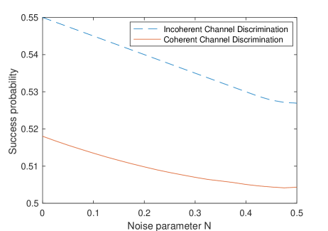
Figure 5: Comparison of the success probabilities of coherent and incoherent channel discrimination for a generalized amplitude damping channel with damping parameter $\gamma=0.2$ and another with damping parameter $\gamma=0.3$. The channels have the same value of the noise parameter $N$, which is varied in the plot.

In this final appendix, I perform a comparison of the success probability of coherent and incoherent channel discrimination for generalized amplitude damping channels. The generalized amplitude damping channel is a simple model of relaxation and thermal noise that can affect a qubit [27]. It is governed by a damping parameter $\gamma\in[0,1]$ and a noise parameter $N\in[0,1]$. When the noise parameter $N=0$, it reduces to the standard amplitude damping channel. It is defined by the following four Kraus operators [27]:

$$\sqrt{1-N}\left(|0\rangle\langle 0|+\sqrt{1-\gamma}|1\rangle\langle 1|\right),$$ (93)

$$\sqrt{\gamma(1-N)}|0\rangle\langle 1|,$$ (94)

$$\sqrt{N}\left(\sqrt{1-\gamma}|0\rangle\langle 0|+|1\rangle\langle 1|\right),$$ (95)

$$\sqrt{\gamma N}|1\rangle\langle 0|.$$ (96)

Using these Kraus operators and the semi-definite programming formulation of the success probability of coherent channel discrimination from (25), we can calculate it for generalized amplitude damping channels (Matlab files for doing so are available with the arXiv posting of this paper). We can also calculate the success probability of incoherent channel discrimination of the same channels by using the semi-definite programming formulation of the diamond distance from [14] and combining with (8).

Figures 4 and 5 compare the success probabilities of coherent and incoherent channel discrimination for generalized amplitude damping channels with different values of the damping parameter $\gamma$ and the noise parameter $N$.

References

[1]
A. Y. Kitaev, “Quantum computations: algorithms and error correction,”
Russian Mathematical Surveys, vol. 52, no. 6, pp. 1191–1249, Dec.
1997.
[2]
D. Aharonov, A. Kitaev, and N. Nisan, “Quantum circuits with mixed states,”
in Proceedings of the thirtieth annual ACM Symposium on Theory of
Computing. New York, NY, USA: ACM,
May 1998, pp. 20–30, arXiv:quant-ph/9806029.
[3]
A. M. Childs, J. Preskill, and J. Renes, “Quantum information and precision
measurement,” Journal of Modern Optics, vol. 47, no. 2–3, pp.
155–176, Jul. 2000, arXiv:quant-ph/9904021.
[4]
A. Acin, “Statistical distinguishability between unitary operations,”
Physical Review Letters, vol. 87, no. 17, p. 177901, Oct. 2001,
arXiv:quant-ph/0102064.
[5]
B. Rosgen and J. Watrous, “On the hardness of distinguishing mixed-state
quantum computations,” Proceedings of the 20th IEEE Conference on
Computational Complexity, pp. 344–354, Jun. 2005, arXiv:cs/0407056.
[6]
A. Gilchrist, N. K. Langford, and M. A. Nielsen, “Distance measures to compare
real and ideal quantum processes,” Physical Review A, vol. 71, no. 6,
p. 062310, Jun. 2005, arXiv:quant-ph/0408063.
[7]
M. F. Sacchi, “Optimal discrimination of quantum operations,” Physical
Review A, vol. 71, no. 6, p. 062340, Jun. 2005, arXiv:quant-ph/0505183.
[8]
——, “Entanglement can enhance the distinguishability of
entanglement-breaking channels,” Physical Review A, vol. 72, no. 1,
p. 014305, Jul. 2005, arXiv:quant-ph/0505174.
[9]
P. Aliferis, Quantum Error Correction. Cambridge University Press, 2013, ch. Introduction to Quantum
Fault Tolerance, pp. 114–144.
[10]
T. Vidick and J. Watrous, “Quantum proofs,” Foundations and Trends in
Theoretical Computer Science, vol. 11, no. 1–2, pp. 1–215, 2016,
arXiv:1610.01664.
[11]
D. Kretschmann and R. F. Werner, “Tema con variazioni: quantum channel
capacity,” New Journal of Physics, vol. 6, no. 1, p. 26, 2004,
arXiv:quant-ph/0311037.
[12]
B. Rosgen, “Computational distinguishability of quantum channels,” Ph.D.
dissertation, University of Waterloo, Sep., 2009, arXiv:0909.3930.
[13]
S. Lloyd, “Enhanced sensitivity of photodetection via quantum illumination,”
Science, vol. 321, no. 5895, pp. 1463–1465, Sep. 2008,
arXiv:0803.2022.
[14]
J. Watrous, “Semidefinite programs for completely bounded norms,”
Theory of Computing, vol. 5, no. 11, pp. 217–238, Nov. 2009,
arXiv:0901.4709.
[15]
A. Harrow, “Coherent communication of classical messages,” Physical
Review Letters, vol. 92, no. 9, p. 097902, Mar. 2004,
arXiv:quant-ph/0307091.
[16]
——, “Entanglement spread and clean resource inequalities,” XVIth
International Congress on Mathematical Physics, pp. 536–540, 2010,
arXiv:0909.1557.
[17]
S. Das, S. Bäuml, and M. M. Wilde, “Entanglement and secret-key-agreement
capacities of bipartite quantum interactions and read-only memory devices,”
December 2017, arXiv:1712.00827.
[18]
A. A. Abbott, J. Wechs, D. Horsman, M. Mhalla, and C. Branciard,
“Communication through coherent control of quantum channels,” Oct. 2018,
arXiv:1810.09826.
[19]
P. A. Guérin, G. Rubino, and C. Brukner, “Communication through
quantum-controlled noise,” Physical Review A, vol. 99, no. 6, p.
062317, Jun. 2019, arXiv:1812.06848.
[20]
L. M. Procopio, F. Delgado, M. Enriquez, N. Belabas, and J. A. Levenson,
“Communication enhancement through quantum coherent control of channels
in an indefinite causal-order scenario,” Feb. 2019, arXiv:1902.01807.
[21]
Q. Dong, S. Nakayama, A. Soeda, and M. Murao, “Controlled quantum operations
and combs, and their applications to universal controllization of divisible
unitary operations,” Nov. 2019, arXiv:1911.01645.
[22]
S. Khatri, R. LaRose, A. Poremba, L. Cincio, A. T. Sornborger, and P. J. Coles,
“Quantum-assisted quantum compiling,” Quantum, vol. 3, p. 140, May
2019, arXiv:1807.00800.
[23]
K. Sharma, S. Khatri, M. Cerezo, and P. J. Coles, “Noise resilience of
variational quantum compiling,” Aug. 2019, arXiv:1908.04416.
[24]
M. M. Wilde, Quantum Information Theory. Cambridge University Press, Feb. 2017, arXiv:1106.1445v8.
[25]
C. H. Bennett, “Logical reversibility of computation,” IBM Journal of
Research and Development, vol. 17, no. 6, pp. 525–532, Nov. 1973.
[26]
——, “Time/space trade-offs for reversible computing,” SIAM Journal
on Computing, vol. 18, no. 4, pp. 766–776, Aug. 1989.
[27]
M. A. Nielsen and I. L. Chuang, Quantum Computation and Quantum
Information. Cambridge University
Press, 2000.
[28]
G. Gour, “Comparison of quantum channels with superchannels,” IEEE
Transactions on Information Theory, vol. 65, no. 9, pp. 5880–5904, Sep.
2019, arXiv:1808.02607.
[29]
G. Chiribella, G. M. D’Ariano, and P. Perinotti, “Transforming quantum
operations: Quantum supermaps,” Europhysics Letters, vol. 83, no. 3,
p. 30004, Aug. 2008, arXiv:0804.0180.
[30]
A. Kitaev and J. Watrous, “Parallelization, amplification, and exponential
time simulation of quantum interactive proof systems,” in Proceedings
of the 32nd ACM Symposium on Theory of Computing, May 2000, pp. 608–617.
[31]
V. Paulsen, Completely Bounded Maps and Operator Algebras, ser.
Cambridge Studies in Advanced Mathematics. Cambridge University Press, 2003.
[32]
A. S. Holevo, Quantum systems, channels, information: A mathematical
introduction. Walter de Gruyter,
2012.