Mean-field density of states of a small-world model and a jammed soft spheres model

Abstract

We consider a class of random block matrix models in $d$ dimensions, $d\geq 1$, motivated by the study of the vibrational density of states (DOS) of soft spheres near the isostatic point. The contact networks of average degree $Z=z_{0}+\zeta$ are represented by random $z_{0}$-regular graphs (only the circle graph in $d=1$ with $z_{0}=2$) to which Erdös-Renyi graphs having a small average degree $\zeta$ are superimposed.

In the case $d=1$, for $\zeta$ small the shifted Kesten-McKay DOS with parameter $Z$ is a mean-field solution for the DOS. Numerical simulations in the $z_{0}=2$ model, which is the $k=1$ Newman-Watts small-world model, and in the $z_{0}=3$ model lead us to conjecture that for $\zeta\to 0$ the cumulative function of the DOS converges uniformly to that of the shifted Kesten-McKay DOS, in an interval $[0,\omega_{0}]$, with $\omega_{0}<\sqrt{z_{0}-1}+1$.

For $2\leq d\leq 4$, we introduce a cutoff parameter $K_{d}\leq 0.5$ modeling sphere repulsion. The case $K_{d}=0$ is the random elastic network case, with the DOS close to the Marchenko-Pastur DOS with parameter $t=\frac{Z}{d}$. For $K_{d}$ large the DOS is close for small $\omega$ to the shifted Kesten-McKay DOS with parameter $t=\frac{Z}{d}$; in the isostatic case the DOS has around $\omega=0$ the expected plateau. The boson peak frequency in $d=3$ with $K_{3}$ large is close to the one found in molecular dynamics simulations for $Z=7$ and $8$. Keywords: random matrix theory, small-world, jamming, boson peak

I Introduction

The spectral distribution of the vibrational modes of disordered solids is not yet completely understood, in particular the origin of the sharp increase of the vibrational density of states (DOS) $D(\omega)$ at small frequency, around the frequency identified as the ”boson peak” in $\frac{D(\omega)}{\omega^{d-1}}$, which gives a comparison between $D(\omega)$ and the Debye law $D(\omega)\sim\omega^{d-1}$, where $d$ is the dimension.

Modeling a disordered solid with frictionless soft spheres with repulsive finite range potentials, in ohern it has been found in computer simulations that at the jamming threshold $D(\omega)$ has a plateau around zero frequency, and that the network of contacts has average coordination degree $Z$ equal to $Z_{c}=2d$. This excess of low energy modes is related to the condition of isostaticity introduced by Maxwell maxwell , balancing the number of degrees of freedom of the particles with the constraints between them. In the hyperstatic region, in which $Z>2d$ and $\delta Z\equiv Z-2d$ is small, there is a boson peak. In wnw it is argued, based on the Maxwell condition, that the sharp increase in $D(\omega)$ is a common feature of weakly-connected amorphous solids.

In crystals a sharp increase in the DOS occurs at a van Hove singularity, which occurs at high frequencies, related to the short-range properties of the crystal. The boson peak seems to have some characteristics typical of long-range properties (occurring at small frequency) and short-range properties. It has been suggested that the boson peak is a shifted van Hove singularity tar .

In MZ a local inversion-symmetry breaking parameter has been found to be relevant for the boson peak; it is sensitive to the angular correlation between bonds connecting spheres.

In ML it has been observed that random matrix models with translational invariance give a possible simple model of the boson peak.

Random block matrix models on random regular graphs have been studied in pari1 , to give a simple mean-field approximation of the random network of contacts, in which the versors pointing from a node to another are independent and randomly uniformly distributed in $d$ dimensions. In that paper it has been shown that, for $d\to\infty$, the spectral distribution of the Hessian matrix for an elastic network on random regular graphs is the Marchenko-Pastur (MP) distribution. This model has been studied in pari1 ; benetti in $d=3$ using the cavity method and exact diagonalization, together with a class of models ${\cal G}_{(z_{0},\zeta)}$ in which the random graphs with average degree $Z=z_{0}+\zeta$ are formed superimposing Erdös-Renyi random graphs of degree $\zeta$ to random regular graphs of degree $z_{0}$. In benetti it has been remarked that, due to the tree-like nature of the random regular graphs, Goldstone modes are absent, so there are no phonons, but only strongly-scattered modes. They find that in the isostatic case the DOS has a peak for zero frequency, possibly a logarithmic divergence, instead of having a plateau. In the hyperstatic case ${\cal G}_{(7,0)}$ in $d=3$ their numerical simulations show that there is a quasi-gap with $D(\omega)\sim\omega^{4}$ for $\omega\to 0$, predicted in gurev and found in molecular dynamics simulations in ler ; miz ; kap .

The method of the spectral distribution moments for random block matrix models on random Erdös-Renyi graphs has been studied in CKMZ , where it was conjectured that the spectral distribution in the limit $d\to\infty$, with $\frac{Z}{d}$ fixed, is the MP distribution. This conjecture has been proved in CP .

Another class of models characterized by the interplay between short-range properties and long-range properties are the small-world models ws ; nw . In particular a mean-field analytic form for the distribution of path lengths has been found nmw in the $k=1$ Newman-Watts small-world model nw , a ring with a small number of random shortcuts; this mean-field solution tends to be exact in the limit of a large number of nodes and few shortcuts. Various properties of the vibrational spectrum of this model have been studied: the effective medium approximation (EMA) spectrum density for this model for small $\omega$ is given in monasson ; the lowest non-zero eigenvalue of the laplacian matrix, known as the algebraic connectivity fiedler has been studied in olf ; gu ; a lower bound on it is given in gu . The laplacian spectral distribution for this small-world model is discussed in olf .

The spectral distribution of the adjacency matrix of an uniformly distributed random $t$-regular graph has been found in kesten ; MK ; shifting it one obtains the spectral distribution of the corresponding laplacian matrix, and hence the DOS of a random regular elastic network in $d=1$. We will indicate in the following with $D_{K}(\omega;t)$ the shifted Kesten-McKay DOS (SKM DOS) with parameter $t$.

In this paper we study the DOS of the laplacian random block matrix for ${\cal G}_{(z_{0},\zeta)}$ models in various dimensions; for $d=1$ it is the laplacian matrix of a random graph, for $d>1$ the blocks are, as in benetti ; CKMZ , $d$-dimensional projectors defined by the random $d$-dimensional contact versor between two sites.

In section II we review the random elastic network model. Using CP we give a new proof that in the case of a random regular graph network of degree $Z$ in $d$ dimensions, in the limit $d\to\infty$ and $t=\frac{Z}{d}$ fixed one obtains the MP distribution with parameter $t$.

In section III we argue that in the ${\cal G}_{(z_{0},\zeta)}$ model in $d=1$, with average degree $t=z_{0}+\zeta$, for $\zeta$ small the density of state is well approximated by the SKM DOS with parameter $t$, by giving a mean-field argument, based on the corresponding derivation for the random regular graphs wanless . Numerical simulations in the cases $z_{0}=2$ and $3$ lead us to conjecture that for $\zeta\to 0$ the cumulative function of the DOS tends uniformly to the one of the SKM DOS, in an interval $[0,\omega_{0}]$, with $\omega_{0}<\sqrt{z_{0}-1}+1$. The ${\cal G}_{(2,\zeta)}$ model is the $k=1$ Newman-Watts small-world model.

In section IV we introduce a model for jammed soft spheres; it differs from the random network model by the introduction of a cutoff parameter $K_{d}$ representing sphere repulsion in an equilibrium configuration: in its absence ($K_{d}=0$) one has the random network model studied in pari1 ; benetti , in which the contact versors are independent random variables, uniformly distributed in $d$ dimensions; for $0<K_{d}\leq 0.5$ two random versors $v,w$ representing the directions of the contacts of a sphere with two other spheres satisfy the bound $v\cdot w\leq 1-K_{d}$.

Numerical simulations in $d=2,3,4$ indicate that, in the isostatic case ${\cal G}_{(2d,0)}$ the peak of $D(\omega)$ in $\omega=0$, present for $K_{d}=0$, becomes with the increase of $K_{d}$ the expected plateau.

We find that in the ${\cal G}_{(z_{0},\zeta)}$ models in $1\leq d\leq 4$, with large cutoff $K_{d}$ for $2\leq d\leq 4$, $D(\omega)$ is well approximated for $\omega<1.5$ by the SKM DOS $D_{K}(\omega;\frac{Z}{d})$, apart from a long tail around $\omega=0$ in $d=1$. This is to be contrasted with the $K_{d}=0$ case, with $d=2,3,4$, in which the DOS is much closer to the MP DOS than to the SKM DOS. Therefore the parameter $K_{d}$ allows an interpolation between a case close the $d=1$ solution (SKM) and a case close to the $d=\infty$ solution (MP). In the $d=3$, $Z=7$ and $8$ hyperstatic cases, the boson peak frequencies corresponding to the SKM DOS are close to the values found in molecular dynamics simulation in MZ .

For $K_{d}$ large, the quantity $\frac{D(\omega)}{\omega^{2}}$, whose peak is the boson peak in the $d=3$ model, is well approximated by $\frac{D_{K}(\omega;\frac{Z}{d})}{\omega^{2}}$.

For $2\leq d\leq 4$ we find that there is a gap in $D(\omega)$ close to the one in $D_{K}(\omega;\frac{Z}{d})$; the quasi-gap found in benetti in $d=3$ with $D(\omega)\approx\omega^{4}$ for $\omega\to 0$ in the hyperstatic case $Z=7$ becomes a gap in presence of a large cutoff $K_{3}$.

In section II we review the network model for soft-spheres near jamming. In section III we study the $d=1$ models, including the $k=1$ Newman-Watts small-world model. In section IV we study the soft-sphere model with angular cutoff.

II Random block matrix model for a random elastic network

Consider a system of $N$ soft spheres in $d$ dimensions, with centers in $r_{i}$, $i=1,\cdots,N$. We assume that the spheres interact with a short-range repulsive central potential. Following pari1 ; benetti , to an equilibrium configuration of spheres a network of contacts is associated, where an edge $(i,j)$ is present if the sphere in $r_{i}$ is in contact with the sphere in $r_{j}$. Let $v_{i,j}=r_{j}-r_{i}$; $\hat{v}_{i,j}$ is the corresponding versor. In a random elastic network the contact versors are random independent uniformly distributed $d$-dimensional Gaussian versors.

Define $X_{i,j}=|\hat{v}_{i,j}><\hat{v}_{i,j}|$. In the elastic approximation, in which displacements $r_{i}\to r_{i}+\delta_{i}$ are kept only to quadratic order, the energy of the system is, neglecting the ”initial-stress” contribution,

$$E=\sum_{i,j}\delta_{i}\cdot M_{i,j}\cdot\delta_{j}$$ (1)

where $M_{i,j}$ is the Hessian,

$$M_{i,j} = -\alpha_{i,j}X_{i,j},\qquad i\neq j=1,\cdots,N$$

$$M_{i,i} = \sum_{j\neq i}\alpha_{i,j}X_{i,j}$$ (2)

with $\alpha_{i,j}$ element of the adjacency matrix of the network graph. $M$ has eigenvalues $\lambda=\omega^{2}$, where $\omega$ is the frequency.

The density of states is

$$D(\omega)=2\omega\rho(\omega^{2})$$ (3)

where $\rho(\lambda)$ is the spectral density.

The Maxwell isostatic condition is $Z_{c}=2d$; $Z$ is the average coordination degree.

In ohern it has been observed that jamming occurs at the isostatic point; the density of states $D(\omega)$ has a plateau around $\omega=0$. Close to the jamming point they found with numerical simulations that $Z-Z_{c}\propto(\phi-\phi_{c})^{\frac{1}{2}}$, $\phi$ being the packing fraction and $\phi_{c}$ the jamming packing fraction. Therefore $Z$ plays a similar role to the packing fraction.

In a physical network of contacts the coordination numbers should be close to the average degree $Z$. In pari1 the network of contacts has been chosen to be random regular graphs.

The exact DOS for these models for arbitrary $d$ is not known; the $d=1$ random regular graph case is obtained from the Kesten-McKay distribution; it is reviewed in section III.

The $d\to\infty$ random regular graph model, with $t=\frac{Z}{d}$ fixed, gives the MP distribution pari1 . Let us give a new proof of this, using CP .

The contributions to the spectral moments are given, in the limit $N\to\infty$, by tree walks. In the case of random regular graphs of degree $Z$, the walks are on the Bethe lattice of degree $Z$.

Consider the unoriented graph on which the walk is embedded. It has the root of degree $\delta_{0}$ and the other nodes $i$ of degree $\delta_{i}$.

Starting from the root, the first edge can be chosen in $Z$ ways; when the path returns to the root, an edge different from the one previously taken can be chosen in $Z-1$ ways, and so on, so one gets a factor $Z^{\underline{\delta_{0}}}$, where $n^{\underline{i}}$ is the falling factorial. When the path arrives at the node $i$ different from the root, there is at that node at least an edge already visited, so that one gets a factor $(Z-1)^{\underline{\delta_{i}-1}}$.

Therefore there is a combinatorial factor associated to the walk on the Bethe lattice

$$Z^{\underline{\delta_{0}}}\prod_{i}(Z-1)^{\underline{\delta_{i}-1}}$$ (4)

In the limit $d\to\infty$ with $t=\frac{Z}{d}$ fixed, the $Z-i$ factors can be approximated with $Z$ at leading order, so one gets a factor $Z^{E}$, where $E$ is the number of edges in the tree associated to the walk. Then one gets the same power of $Z$ that one gets from the same walk in the Erdös-Renyi model, in the limit $N\to\infty$. In that case the $Z$ factors come from the probability distribution of the adjacency matrix weights.

The average on the blocks $X_{i,j}$ associated to the steps of the walk is the same in the Erdös-Renyi and in the random regular graph cases; in the limit $d\to\infty$ it gives to leading order a factor $d^{-E}$; putting the two factors together one gets a factor $t^{E}$.

Therefore in the limit $N\to\infty$, $d\to\infty$ with $t=\frac{Z}{d}$ fixed one gets the same spectral moments in the two models. Since in CP it has been proved that in the case of Erdös-Renyi graphs the spectral distribution is the MP distribution, the same holds for the case of random regular graphs.

To the MP distribution corresponds the density of states

$$D_{M}(\omega;t) = \frac{1}{2\pi\omega}\sqrt{(b^{2}-\omega^{2})(\omega^{2}-a^{2})}$$

$$a = \sqrt{t}-\sqrt{2}\,;\qquad b=\sqrt{t}+\sqrt{2}$$ (5)

for $a\leq\omega\leq b$ and zero otherwise.

In CKMZ it has been observed that the random block matrix model with Erdös-Renyi contact network interpolates between the $d=1$ model with coordination degree $t$ and the $d\to\infty$ model with coordination degree $t=\frac{Z}{d}$. In CP it has been proved that the non-crossing contributions to the spectral moments depend only on $t$, so they are common to the models with different $d$, but same $t=\frac{Z}{d}$. The crossing contributions depend on $t$ and $d$; they vanish in the $d\to\infty$ limit. In CKMZ simulations show that, for $d>1$, the spectral distribution is fairly well approximated by the one for $d\to\infty$, the MP distribution with parameter $t$, so the crossing contributions seem to have a small effect.

The $d=1$ spectral distribution differs markedly from the MP DOS, due to a series of spikes. Its analytical form is unknown.

The Kesten-McKay distribution has been derived in kesten ; MK for $t$-regular random graphs, hence with $t$ integer. In the next section we will discuss $d=1$ models, which have as mean-field DOS the SKM DOS with $t$ real.

The uniformity of the DOS of the Erdös-Renyi models with different $d$ and $t=\frac{Z}{d}$ fixed, leads us to examine with simulations whether the same happens in the case of random regular graphs, and to see whether in the latter case the DOS is closer to the $d=1$ SKM DOS or the $d\to\infty$ Marchenko-Pastur DOS, both with parameter $t$. In section IV we will see that in the elastic network model the DOS is close to the MP DOS with parameter $t$, while in a soft sphere model with large angular cutoff, modeling the repulsion between spheres in an equilibrium configuration, the DOS is close to the SKM DOS with parameter $t$.

III $d=1$ models

III.1 Kesten-McKay distribution and ${\cal G}_{(z_{0},\zeta)}$ models

The Kesten-McKay distribution kesten ; MK is the spectral distribution of the Adjacency matrix $A$ of random uniformly distributed regular graphs of degree $t$, in the limit of number of nodes going to infinity.

Let us review here a derivation of this distribution wanless .

In the limit of number of nodes $N$ going to infinity, the moment of the spectral distribution $\mu_{n}=\frac{1}{N}\langle trA^{n}\rangle$ is the number of walks of length $n$ on a Bethe lattice of degree $t$.

Consider an infinite rooted tree with root of degree $s$ and all the other nodes of degree $t$. Let $T_{s}^{(t)}(x)$ be the generating function of the number of tree walks of length $n$ starting at the root; $T_{s}^{(t)}(0)=1$. A non-trivial walk starting at the root can go from the root to a neighbor node in $s$ ways; then it can take a walk not returning to the root; then it returns to the root. From there it can take another tree walk. One has therefore

$$T_{s}^{(t)}-1=x^{2}sT_{t-1}^{(t)}T_{s}^{(t)}$$ (6)

Taking the case $s=t-1$ in this equation, one obtains a quadratic equation, whose root is determined by the condition $T_{t-1}^{(t)}(0)=1$. Substituting this in Eq. (6), in the case $s=t$ one gets

$$T_{t}^{(t)}(x)=\frac{t-2-t\sqrt{1-4x^{2}(t-1)}}{2(x^{2}t^{2}-1)}$$ (7)

The resolvent of the adjacency matrix is

$$r_{A}(z)=\sum_{n\geq 0}\mu_{n}z^{-n-1}=\frac{1}{z}T_{t}^{(t)}(\frac{1}{z})$$ (8)

From

$$\rho_{A}(x)=-\frac{1}{\pi}\lim_{\epsilon\to 0^{+}}\texttt{Im}\,r_{A}(x+i\epsilon)$$ (9)

one gets the spectral density of the adjacency matrix

$$\rho_{A}(z)=\frac{t}{2\pi}\frac{\sqrt{4(t-1)-z^{2}}}{t^{2}-z^{2}}$$ (10)

for $|z|\leq 2\sqrt{t-1}$ and $0$ otherwise.

The Laplacian matrix differs from $-A$ only by $t$ times the unit matrix, so that its spectral distribution is obtained shifting by $t$ the one in Eq.(10). The density of states is related to the Laplacian spectral density by $D(\omega)=2\omega\rho(\omega^{2})$, $z=\omega^{2}$ so that the corresponding SKM density of states is

$$D_{K}(\omega;t)=\frac{t\omega}{\pi}\frac{\sqrt{4(t-1)-(\omega^{2}-t)^{2}}}{t^{2}-(\omega^{2}-t)^{2}}$$ (11)

for $\sqrt{t-1}-1<\omega<\sqrt{t-1}+1$, zero otherwise.

For $t\geq 3$ this is the density of states for random $t$-regular graphs. For $t=2$ it is the density of states for the ring

$$D_{K}(\omega;2)=\frac{2}{\pi\sqrt{4-\omega^{2}}}$$ (12)

While the SKM distribution holds exactly for random regular graphs, we argue that for a class of tree-like random graphs with average degree $t$ real it gives a good approximation to the density of states. We consider a class of models ${\cal G}_{(z_{0},\zeta)}$, with average degree $t=z_{0}+\zeta$, in which the random graphs are obtained from a regular graph (a ring for $z_{0}=2$, a randomly distributed $z_{0}$-regular graph for $z_{0}\geq 3$), to which a Erdös-Renyi graph of small average degree $\zeta$ is superimposed. The degree of each vertex $i$ of the graph is $z_{i}=z_{0}+\zeta_{i}$, where $\zeta_{i}$ is a Poisson random variable having mean $\zeta$. The degree distribution of each vertex is $p_{k}=\zeta^{k-z_{0}}\frac{e^{-\zeta}}{(k-z_{0})!}$ for $k\geq z_{0}$, zero otherwise benetti .

Let us consider, similarly to the case of random regular graphs, the generating function $T_{s}^{(t)}$ of the average number of tree walks of length $n$, starting from the root with average degree $s$, the other nodes with average degree $t$; thus $s$ and $t$ are now real quantities.

A non-trivial walk starting at the root can go from the root to a neighbor node in $s$ ways; then it can take a walk not returning to the root; then it returns to the root. From there it can take another tree walk.

In a mean-field approximation one obtains again Eq.(6), where now $s$ and $t$ are average degrees, and from it the spectral density for the Adjacency matrix Eq.(10). For $\zeta$ small, the degrees are close to $t$, so approximatively the Laplacian matrix is $tI-A$, so that one obtains approximatively the density of states $D_{K}(\omega;t)$ in Eq.(11), where $t$ is the average degree, with $t=z_{0}+\zeta$. As $\zeta$ approaches zero, this approximation can be expected to become more accurate.

Due to the fluctuations in numerical simulations for $D(\omega)$, it is convenient to use the cumulative function

$$\Phi(\omega)=\int_{0}^{\omega}d\omega D(\omega)$$ (13)

and similarly $\Phi_{K}(\omega)$ and $\Phi_{M}(\omega)$ respectively for the SKM and the MP DOS.

III.2 Density of states for the $k=1$ Newman-Watts small-world model

In the case $z_{0}=2$, $t=2+\zeta$, the random graphs are defined as a circle graph with $N$ nodes, to which a Erdös-Renyi graph of average degree $\zeta$ is superimposed.

This model belongs to the class of Newman-Watts models, in which the random graph is formed by a ring on $N$ nodes, each node being connected to $2k$ nearest neighbors; an Erdös-Renyi graph is superimposed to it nw . In the $k=1$ Newman-Watts model, in nmw they have computed an analytic expression for the distribution of the distance between nodes, for $\zeta$ small. They obtain it considering a mean-field approximation, in which the average of the distributions on the random graphs is considered. For $\zeta\to 0$ this approximation becomes exact.

We find a similar behavior for the DOS, where $D_{K}(\omega;2+\zeta)$ is the mean-field approximation.

A discussion of the spectrum of the Laplacian for the $k$-small-world models is done in monasson , with emphasis on the simulations in the $k=3$ small-world model. The $k=1$ small-world model is briefly mentioned there, giving the EMA approximation

$$D_{E}(\omega;\zeta)=\frac{\sqrt{8\omega^{2}-\zeta^{2}}}{2\pi\omega}$$ (14)

to which corresponds the cumulative function $\Phi_{E}(\omega)$.

We make numerical simulations to see how the DOS tends to the SKM DOS for $\zeta\to 0$.

In the simulations in this section we used $200$ random graphs with $3000$ nodes, unless specified. The eigenvalues of the laplacian matrix are computed using in Sagemath sage the function Numpy.linalg.eigvalsh.

In Fig. 1 the cumulative function is given for the case ${\cal G}_{(2,0.01)}$; in the left hand figure are plotted $\Phi$, $\Phi_{K}$, $\Phi_{M}$ and $\Phi_{E}$. $\Phi$ has a high frequency (HF) tail, with $\omega>\sqrt{t-1}+1$, beyond the support of the SKM DOS. In $\omega=2.1976(3)$ the DOS has a spike (see Fig. 8 and its note), giving a dent in $\Phi$, visible in Fig. 1. In the right hand figure the cumulative functions for $\zeta=0.01$ are given for small $\omega$; $\Phi$ starts with the zero-mode contribution.

In the left hand figure in Fig. 2 are given the areas under $D(\omega)$ in the HF tails, for a few values of $\zeta$ between $0.005$ and $0.1$; they fit with $0.50\zeta$, so they should go to zero approximately at this rate.

The DOS has a van Hove peak tending to $2$ for $\zeta\to 0$: its frequency is $1.9987(3)$ for $\zeta=0.1$, $1.9998(3)$ for $\zeta=0.01$; the uncertainty is due to the fact that we used bins of size $\Delta\omega=10^{-3.5}$.

In the center figure in Fig. 2, $\Phi(\omega)-\Phi_{K}(\omega)$ is plotted for a few values of $\zeta$ between $\zeta=0.01$ and $0.1$. For $\omega>1.8$ there is a sharp increase in this difference, due to the fact that the DOS has the van Hove peak slightly less than $2$, while the SKM DOS has a van Hove peak at slightly less than $\sqrt{t-1}+1$.

$\Phi$ starts at $\omega=0$ with the zero mode; $\Phi(0)$ goes to zero for $N\to\infty$; with the increase of $N$, $\Phi$ has fewer fluctuations; in the right hand side figure in Fig. 2 we give $\Phi(\omega)-\Phi_{K}(\omega)$ for $\zeta=0.01$, $N=500$ and $N=3000$.

The area of the high-frequency tail does not change with $N$; e.g. for $\zeta=0.01$ it is equal to $0.005$ for $N=500$, $1000$ and $3000$.

In the center figure in Fig. 8 for $t=2.01$, and Fig. 9 for $t=7/3$, one can see a difference also for $\omega$ small, where $D_{K}(\omega;t)$ is zero for $\omega\leq\sqrt{t-1}-1$, while $D(\omega)$ has a tail going much closer to zero. The smallest nonzero eigenvalue of the laplacian is the algebraic connectivity $\lambda_{2}=\omega_{2}^{2}$; it has been studied in olf ; gu ; in gu it has been shown to go slowly to zero for $N\to\infty$.

These simulations lead us to conjecture that the DOS tends to the SKM DOS for $\zeta\to 0$ in the following way: for $N\to\infty$, $\Phi$ converges uniformly as $\zeta\to 0$ to $\Phi_{K}$ for $\omega\leq\omega_{0}$, with $\omega_{0}<2$; the area of the high-frequency tail, with $\omega>\sqrt{1+\zeta}+1$, goes to zero linearly for $\zeta\to 0$. In the interval $[\omega_{0},\sqrt{1+\zeta}+1]$ there are the van Hove peak of the SKM DOS and the one of the DOS, tending to each other for $\zeta\to 0$.

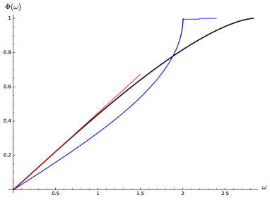
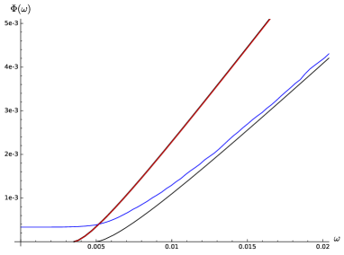
Figure 1: In the left hand figure $\Phi(\omega)$ for $t=2.01$ is plotted in blue, the SKM in black (thin line) and the MP DOS as a thick black line. The EMA DOS is plotted for $\omega<1.5$, in red. In the right hand figure, they are plotted for small $\omega$; the EMA DOS is very close to the MP DOS.

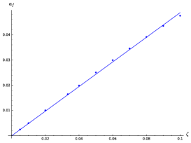
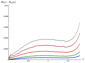
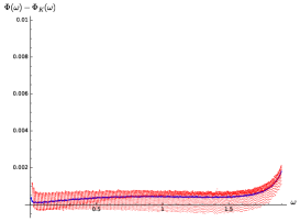
Figure 2: In the case ${\cal G}_{(2,\zeta)}$, the left hand figure shows the area $a_{f}$ under $D(\omega)$ in the HF tail for various values of $\zeta$ between $0.005$ and $0.1$, for $N=3000$. The center figure shows $\Phi(\omega)-\Phi_{K}(\omega)$ for $N=3000$, $\zeta=0.01$(blue), $0.02$(green), $0.04$(red), $0.07$(brown) and $0.1$(gray) for $\omega<1.8$. The right hand figure shows $\Phi(\omega)-\Phi_{K}(\omega)$ for $\zeta=0.01$, $N=500$(red) and $N=3000$ (blue).

III.3 ${\cal G}_{(3,\zeta)}$ model

In the ${\cal G}_{(3,\zeta)}$ model the random graphs are formed by random $3$-regular graphs, to which a Erdös-Renyi graph of average degree $\zeta$ is superimposed.

With respect to the $k=1$ Newman-Watts model, the algebraic connectivity $\lambda_{2}$ is larger; in fact in a graph in the class ${\cal G}_{(z_{0},\zeta)}$ one can expect that $\lambda_{2}=\omega_{2}^{2}$ is larger than for a random $z_{0}$-regular graph, for which the SKM DOS has lowest non-zero frequency $\omega_{2}=\sqrt{z_{0}-1}-1$, hence $\sqrt{2}-1$ for $z_{0}=3$.

In the left hand figure in Fig. 3 the cumulative function is given for $\zeta=0.01$; in the right hand figure it is given near $\omega_{2}$.

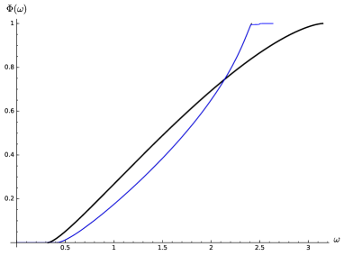
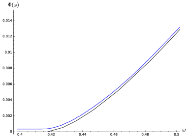
Figure 3: In the left hand figure are given the cumulative functions for the case ${\cal G}_{(3,0.01)}$: $\Phi(\omega)$ (blue), $\Phi_{K}(\omega)$ (thin black), $\Phi_{M}(\omega)$ (thick black). In the right hand figure $\Phi(\omega)$ and $\Phi_{K}(\omega)$ are plotted between $\omega=0.4$ and $\omega=0.5$.

In the left hand figure in Fig. 4 are given the area under $D(\omega)$ in the HF region, i.e. $1-\Phi(\sqrt{t-1}+1)$, for various values of $\zeta$ between $0.01$ and $0.1$; a fit suggests that this area goes to zero as $0.4\zeta$ for $\zeta\to 0$.

In the right hand figure in Fig. 4, $\Phi(\omega)-\Phi_{K}(\omega)$ is plotted for $\omega<2.3$ for a few values of $\zeta$ between $0.01$ and $0.1$; this figure indicates that for $\omega\leq\omega_{0}$, where $\omega_{0}<\sqrt{z_{0}-1}+1$, for $\zeta\to 0$ and $N\to\infty$ the difference $\Phi(\omega)-\Phi_{K}(\omega)$ tends to zero.

Finally both the frequencies of van Hove peak of the SKM DOS and of the one of the DOS tend to $\omega=1+\sqrt{2}$ for $\zeta\to 0$.

We conjecture that for $N\to\infty$, as $\zeta\to 0$ the cumulative function $\Phi$ converges uniformly to $\Phi_{K}$ in an interval $[0,\omega_{0}]$, with $\omega_{0}<\sqrt{z_{0}-1}+1$; that the integral of $D$ over the high frequency region $\omega>\sqrt{z_{0}+\zeta-1}+1$ goes to $0$ in this limit. The frequency of the van Hove peak of the DOS tends to $\sqrt{z_{0}-1}+1$.

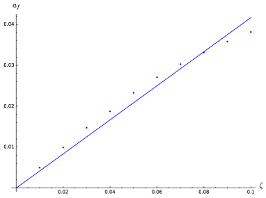
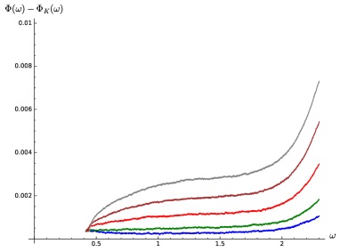
Figure 4: In the case ${\cal G}_{(3,\zeta)}$, the left hand figure shows the area $a_{f}$ under of $D(\omega)$ in the HF tail for various values of $\zeta$ between $0.01$ and $0.1$. The right hand figure shows $\Phi(\omega)-\Phi_{K}(\omega)$ for $\omega<2.3$, for $\zeta=0.01$(blue), $0.02$(green), $0.04$(red), $0.07$(brown) and $0.1$(gray).

IV A random block matrix model for jamming spheres with angular cutoff.

The random elastic network model for jamming soft spheres introduced in pari1 ; benetti and reviewed in section II does not take into account the repulsion between spheres in an equilibrium configuration.

In pari1 ; benetti simulations were made for the random block matrix model for a random elastic network in $d=3$ using random regular graphs. The resulting density of states was found to have, in the isostatic case, a peak in $\omega=0$, instead of the expected plateau; in benetti it is remarked that this peak might be a logarithmic singularity. In the left hand figure in Fig. 5 this density of states is represented by a blue line; it is fairly close to the MP DOS (the thick black line) but, unlike it, it is not flat at $\omega=0$.

In an equilibrium configuration spheres are kept apart by the repulsive force. Let the sphere in $r_{i}$ be in contact with the spheres in $r_{j}$ and $r_{k}$. Due to the repulsion potential spheres in contact are assumed to be roughly at the same distance. To model this in the random block matrix model, we add a parameter $K_{d}$ to the random block matrix model, and the constraints

$$\hat{v}_{i,j}\cdot\hat{v}_{i,k}\leq 1-K_{d}$$ (15)

for all $i,j,k$ such that $\alpha_{i,j}\alpha_{i,k}=1$. For $K_{d}=0$ one recovers the random network model considered previously. For three hard spheres touching each other one has $K_{d}=\frac{1}{2}$, so it is natural to assume $K_{d}\leq\frac{1}{2}$.

For $K_{d}\neq 0$ the contact versors are not anymore independent random versors uniformly distributed in $d$ dimensions. We follow the following algorithm to choose the random versors. In the simulations, to determine random contact versors satisfying this cutoff constraint, we placed random vectors satisfying Eq.(15) with a small cutoff, then we used a greedy algorithm to get random vectors with the required cutoff. We accept the result if the sum, over all sampled networks, of the violations to the required cutoff is less than $0.1$.

All the simulations in $d=3$ are made with 200 random graphs with $1000$ nodes.

In Fig. 5 there is the DOS in the isostatic $d=3$ case, with a few values of $K_{3}$ from $0$ to $0.5$. For $K_{3}=0.5$ there is a plateau around $\omega=0$; this DOS is close to the SKM DOS with parameter $t=2$ (the ring DOS Eq. (12)) for $\omega<1.5$. The density of states with large $K_{3}$ has a plateau for $\omega$ small; with the decrease of $K_{3}$ a peak appears in $\omega=0$; the plateau following the peak is also higher than in the molecular dynamics simulations in ohern . The height of the plateau around $\omega=0$ depends on $K_{3}$; for $K_{3}\simeq 0.3$ it fits with its height in molecular dynamics simulations.

Around $\omega=2$ there is a van Hove peak, which increases in height with $K_{3}$; the SKM DOS has a much higher peak, which is not drawn in the figure.

Let us now consider the hyperstatic cases $Z=7,8$ and $9$ in $d=3$. In the case $K_{3}=0$ the density of states is fairly close to the MP DOS with parameter $t=\frac{Z}{d}$; the DOS’ are displayed in the left hand figure in Fig. 6. For $K_{3}\leq 0.5$ and as large as managed (i.e. $K_{3}=0.5$ for $Z=7$, $K_{3}=0.47$ for $Z=8$ and $K_{3}=0.42$ for $Z=9$), the DOS is close, for $\omega<1.5$, to the SKM DOS with parameter $t=\frac{Z}{d}$. They are plotted in the center hand figure in Fig. 6.

The quasi-gap in $D(\omega)$ for $K_{3}=0$ (estimated in benetti to go as $\omega^{4}$ for $\omega\to 0$), becomes a gap for $K_{3}$ large, as shown in the case $Z=7$ in the right figure in Fig. 6.

In Fig. 7 the corresponding boson peaks are shown.

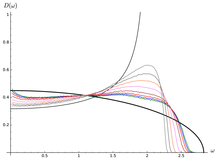
Figure 5: The figure shows $D(\omega)$ in $d=3$ in the isostatic case $Z=6$. Simulations are with $K_{3}=0$ (green), $K_{3}=0.02$(blue), $K_{3}=0.05$(red), $K_{3}=0.1$(brown), $K_{3}=0.2$(violet), $K_{3}=0.3$(coral), $K_{3}=0.4$(dimgray), $K_{3}=0.5$(gray). The smooth black curves are the SKM DOS (thin curve) and the MP DOS (thick curve).

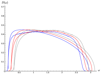
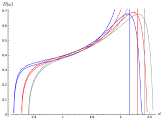
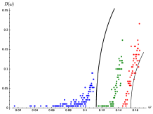
Figure 6: The left side figure shows $D(\omega)$ in $d=3$ for $Z=7$ (blue), $Z=8$ (red) and $Z=9$ (gray) for $K_{3}=0$. The smooth curves of the corresponding colors are for the MP DOS. The center figure shows the DOS in $d=3$ for $Z=7$ (blue), $Z=8$ (red) and $Z=9$ (gray) for $K_{3}=0.5$, $K_{3}=0.47$ and $K_{3}=0.42$ respectively. The smooth curves of the corresponding colors are for the SKM DOS, whose van Hove peaks are not shown beyond height $0.7$. In the right hand figure the $Z=7$ DOS is plotted for small $\omega$, for the case $K_{3}=0$ (red) and $K_{3}=0.2$ (green) and $K_{3}=0$ (blue points). The points are relative at bins of size $\Delta\omega=10^{-3.5}$.

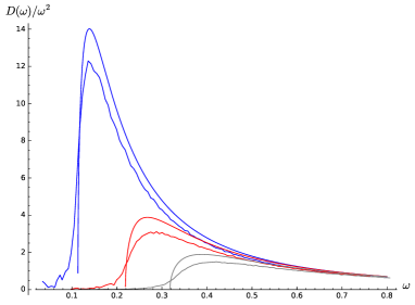
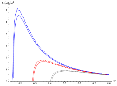
Figure 7: The left side figure shows the boson peak in $d=3$ for $Z=7$ (blue), $Z=8$ (red) and $Z=9$ (gray) for $K_{3}=0$. The smooth curves of the corresponding colors are for the MP DOS. The right side figure shows the boson peak in $d=3$ for $Z=7$ (blue), $Z=8$ (red) and $Z=9$ (gray) for $K_{3}=0.5$, $0.47$ and $0.42$ respectively. The smooth curves of the corresponding colors are for the SKM DOS.

We have seen in a few cases above that in the case of a random $Z$-regular matrix network and with large $K_{3}$ cutoff the DOS is close to $D_{K}(\omega;t)$.

As in benetti , we consider also a class of models with random graphs in ${\cal G}_{(z_{0},\zeta)}$, i.e. random regular graphs of degree $z_{0}$, on which Erdös-Renyi graphs with average degree $\zeta$ are superimposed. This allows to consider real values for $Z=z_{0}+\zeta$. We have already examined the $d=1$ ${\cal G}_{(z_{0},\zeta)}$ models in section III.

With the introduction of a large cutoff $K_{d}\leq 0.5$, the $d=2,3,4$ models turn out to have a DOS closer to that of the $d=1$ model with the same $t$, and hence to the SKM DOS $D_{K}(\omega;t)$, than to the MP DOS.

In Fig. 8 are given the results of simulations in the case $t=\frac{Z}{d}=2.01$. For the case $d=1$ it is the case ${\cal G}_{(2,0.01)}$, which we have discussed in section III. Here we plot its DOS; for $\omega<1.5$, it is close to the SKM DOS and to the DOS of the models with large $K_{d}$ in $d=2$, $3$ and $4$ with the same $t$. The highest values found for the cutoff are $K_{2}=0.4$, $K_{3}=K_{4}=0.5$, using $1500$ nodes in $d=2$, $1000$ nodes in $d=3$ and $750$ nodes in $d=4$; for each case, we make the average on $200$ random graphs.

In Fig. 9 are given the results of simulations in the case $t=7/3$. As in the previous case, the densities of states in different dimensions, for $K_{d}$ large, are close to the SKM DOS, for $\omega<1.5$.

For $t=3$ the DOS for $d=2,3$ and $4$ are close, for $\omega<1.5$, to $D_{K}(\omega;3)$ (see the center figure in Fig.6 for the case $d=3$), which is the DOS of the $d=1$ ${\cal{G}}_{(3,0)}$ model.

Halving the number of nodes and making the average on $400$ graphs we get similar results for the DOS. The maximum values of $K_{d}$ change slowly with $N$; in $d=3$ they are less than $5\%$ higher halving $N$. In $d=2$ the change is greater far form the isostatic point; for $z_{0}=2$ and $\zeta=\frac{1}{3}$ the maximum value of $K_{2}$, halving $N$, is $13\%$ higher. Therefore it can be expected that increasing $N$ it decreases further.

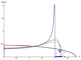
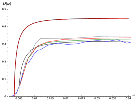
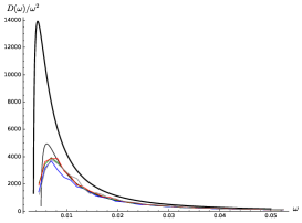
Figure 8: The left side figure shows the DOS for $t=2.01$ for $d=1$ (blue), $d=2$ with $K_{2}=0.4$ (green), $d=3$ with $K_{3}=0.5$ (red) and $d=4$ with $K_{4}=0.5$ (gray). In the case $d=1$ the HF part is not a smooth curve, so points are given, representing bins of width $\Delta\omega=10^{-3.5}$. A point in $(2.1976(3),11.8)$ is not represented in the figure. The center figure shows $D(\omega)$ for small $\omega$ for the same cases. The thin black curve is the SKM DOS, the thick black curve is the MP DOS, the red curve close to it is the EMA DOS in Eq.(14). The right figure shows $\frac{D(\omega)}{\omega^{2}}$ for the same cases.

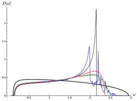
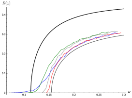
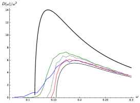
Figure 9: The left side figure shows the density of states for $t=7/3$ for $d=1$ (blue), $d=2$ with $K_{2}=0.16$ (green), $d=3$ with $K_{3}=0.5$ (red) and $d=4$ with $K_{4}=0.5$ (gray). The center figure shows $D(\omega)$ for small $\omega$ for the same cases; the right figure shows $\frac{D(\omega)}{\omega^{2}}$ for the same cases. The thin black curve is the SKM DOS, the thick black curve is the MP DOS.

The curve of the maxima of $\frac{D_{K}(\omega;t)}{\omega^{2}}$ is given by

$$\omega^{6}-\frac{10}{3}t\omega^{4}+\frac{1}{3}(13t^{2}-20t+20)\omega^{2}-8t+8t^{2}-2t^{3}=0$$ (16)

The slope of this curve at the isostatic point $t=2$ is $\frac{\sqrt{6}}{4}$; see the left hand figure in Fig. 10. In it are reported the boson peak frequencies in $d=3$, $Z=7$, $8$ and $9$ found in molecular dynamics simulations in MZ . For $Z=7$ and $8$ these values agree well with the SKM curve, while for $Z=9$ the difference is $4\%$.

In the right hand figure in Fig. 10, $\omega_{BP}$ is plotted against $K_{3}$. There is little difference in $\omega_{BP}$ for $K_{3}=0.3$ and larger values of it.

In the isostatic case we saw that for $K_{3}\simeq 0.3$ the height of the plateau around $\omega=0$ fits with the molecular simulation results in ohern .

Therefore overall $K_{3}\simeq 0.3$ is a good fit in all these cases.

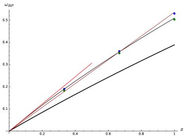
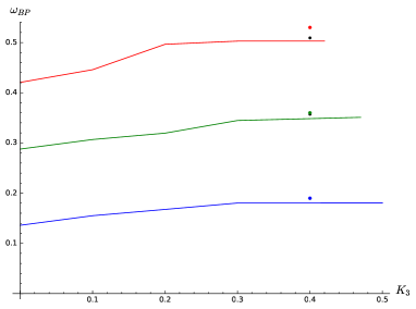
Figure 10: In the left hand figure, the boson peak $\omega_{BP}$ (thin black line) is plotted against $x=t-2$ and its tangent in $x=0$ (red line); $\omega_{BP}$ is computed as the maximum of $\frac{D_{K}(\omega;t)}{\omega^{2}}$. The blue dots are $\omega_{BP}$ in molecular dynamics simulations in MZ for $Z=7,8,9$ in $d=3$; the brown line is a linear fit for these points. The green dots are $\omega_{BP}$ in simulations with largest $K_{3}$. The boson peak for the MP DOS is drawn as a thick black line. In the right hand figure, there is a plot of the boson peak against $K_{3}$; the case $Z=7$ is the line in blue, the case $Z=8$ is the green line, the case $Z=9$ the red line. With the same colors a point indicates the values found in molecular simulations MZ . The black points are the corresponding values from the SKM DOS.

V Conclusion

We find that the shifted Kesten-McKay density of states with parameter $Z=z_{0}+\zeta$ is a mean field solution in a class of random matrix models, based on (random) regular graphs of degree $z_{0}$ to which an Erdös-Renyi graph with small average degree $\zeta$ is superimposed. We conjecture that for $\zeta\to 0$ the cumulative function of the density of states of this model tends uniformly to the one of the mean-field solution, in an interval $[0,\omega_{0}]$, with $\omega_{0}<\sqrt{z_{0}-1}+1$. The $z_{0}=2$ case is the $k=1$ Newman-Watts small-world model.

We introduce a random block matrix model for soft spheres near the jamming point; it differs from the random elastic network model introduced in pari1 ; benetti , due to the introduction of an angular cutoff $K_{d}$ between contact versors, modeling the excluded volume due to sphere repulsion in an equilibrium configuration.

Making simulations in $2\leq d\leq 4$ with the same class of random graphs as above, we find that the density of states in the case of large $K_{d}$ is close to the shifted Kesten-McKay density of states with parameter $t=\frac{Z}{d}$, while in the elastic network case $K_{d}=0$ it is close to the Marchenko-Pastur density of states with parameter $t=\frac{Z}{d}$.

The shifted Kesten-McKay density of states gives in $d=3$, $Z=7$ and $8$ boson peak frequencies in good agreement with molecular dynamics simulations with soft spheres MZ . With respect to the random elastic network model, the large $K_{d}$ model has fewer low-frequency modes; in the isostatic case it has a plateau around $\omega=0$, whose height is for $K_{3}\simeq 0.3$ in agreement with molecular dynamics simulations with soft spheres ohern .

The density of states found in simulations, in the case of large $K_{d}$, has in the hyperstatic case a gap around $\omega=0$, a bit smaller than the one of the shifted Kesten-McKay density of states; therefore $D(\omega)$ does not go as $\omega^{4}$ for $\omega\to 0$. In the elastic network model $K_{d}=0$ there is instead a quasi-gap, for which the behavior $D(\omega)\sim\omega^{4}$ has been found in benetti .

I thank Gianni Cicuta and Alessio Zaccone for discussions.

References

- (1) C.S. O’Hern, L.E. Silbert, A.J. Liu, S.R. Nagel Jamming at zero temperature and zero applied stress: The epitome of disorder, Phys. Rev. E68, 011306 (2003).
- (2) J.C. Maxwell, Philos. Mag. 27, 294 (1864).
- (3) M. Wyart, S. R. Nagel and T.A. Witten, Geometrical origin of excess low-frequency vibrational modes in weakly-connected amorphous solids, Europhys. Lett. 72, 486 (2005).
- (4) S.N. Taraskin, Y.L. Loh, G. Natarajan and S.R. Elliott, Origin of the Boson Peak in Systems with Lattice Disorder, Phys. Rev. Lett. 86, 1255 (2001).
- (5) R. Milkus, A. Zaccone, Local inversion-symmetry breaking controls the boson peak in glasses and crystals, Phys. Rev. B93, 094204 (2016).
- (6) M.L. Manning and A.J. Liu, A random matrix definition of the boson peak, Europhysics Letters 109, 36002 (2015).
- (7) G. Parisi, Soft modes in jammed hard spheres (I): Mean field theory of the isostatic transition, arxiv 1401.4413 (2014).
- (8) F.P.C. Benetti, G. Parisi, F. Pietracaprina, G. Sicuro, Mean-field model for the density of states of jammed soft spheres, Phys. Rev. E97 062157 (2018).
- (9) V. L. Gurevich, D. A. Parshin and H. R. Schober, Anarmonicity, vibrational instability and Boson peak in glasses, Phys. Rev. B67, 094203 (2003).
- (10) E. Lerner, G. Düring, and E. Bouchbinder, Statistics and Properties of Low-Frequency Vibrational Modes in Structural Glasses, Phys. Rev. Lett. 117, 035501 (2016).
- (11) H. Mizuno, H. Shiba and A. Ikeda, Continuum limit of the vibrational properties of amorphous solids, Proc. Natl. Acad. Sci. USA 114, E9767 (2017).
- (12) G. Kapteijns, E. Bouchbinder and E. Lerner, Universal non-phononic density of states in 2D, 3D and 4D glasses, Phys. Rev. Lett. 121, 055501 (2018)
- (13) G. M. Cicuta, J. Krausser, R. Milkus, A. Zaccone, Unifying model for random matrix theory in arbitrary space dimension, Phys. Rev. E 97, 032113 (2018).
- (14) M. Pernici and G. Cicuta, Proof of a conjecture on the infinite dimension limit of a unifying model for random matrix theory, Journal Stat. Phys. 175, 384 (2019).
- (15) D.J. Watts and S.H. Strogatz, Collective dynamics of small-world networks, Nature 393, 440 (1998).
- (16) M.E.J Newman and D.J. Watts, Renormalization group analysis of the small-world network model, Phys. Lett. A 263, 341 (1999).
- (17) M.E.J Newman, C. Moore and D.J. Watts, Mean-field solution of the small-world network model, Phys. Rev. Lett. 84, 3201 (2000).
- (18) R. Monasson, Diffusion, localization and dispersion relations on ”small-world” lattices, Eur. Phys. J. B. 12, 555 (1999).
- (19) M. Fiedler, Algebraic connectivity of graphs, Czech. Math. J. 23, 298 (1973).
- (20) R. Olfati-Saber, Ultrafast consensus in small-world networks, in Proc. 2005 Am. Control Conf., 2371 (2005).
- (21) L. Gu, X.D. Zhang and Q. Zhou, Consensus and synchronization problems on small-world networks, Journ. Math. Phys. 51, 082701 (2010).
- (22) H. Kesten, Symmetric random walks on groups, Trans. Amer. Math. Soc., 92:336 (1959).
- (23) B.D. McKay, The expected eigenvalue distribution of a large regular graph, Linear Algebra Appl. 40, 203 (1981).
- (24) I.M. Wanless, Counting matchings and tree-like walks in regular graphs, Combinatorics, Probability and Computing 19, 463 (2010).
- (25) SageMath, the Sage Mathematics Software System (Version 7.3), The Sage Developers, 2016, https://www.sagemath.org.