On Competitive Analysis for Polling Systems

Abstract

Polling systems have been widely studied, however most of these studies focus on polling systems with renewal processes for arrivals and random variables for service times. There is a need driven by practical applications to study polling systems with arbitrary arrivals (not restricted to time-varying or in batches) and revealed service time upon a job’s arrival. To address that need, our work considers a polling system with generic setting and for the first time provides the worst-case analysis for online scheduling policies in this system. We provide conditions for the existence of constant competitive ratios, and competitive lower bounds for general scheduling policies in polling systems. Our work also bridges the queueing and scheduling communities by proving the competitive ratios for several well-studied policies in the queueing literature, such as cyclic policies with exhaustive, gated or $l$-limited service disciplines for polling systems.

Keywords— Scheduling, Online Algorithm, worst-case Analysis, Competitive Ratio, Parallel Queues with Setup Times

1 Introduction

This study has been motivated by operations in smart manufacturing systems. As an illustration, consider a 3D printing machine that uses a particular material informally called “ink” to print. Jobs of the same prototype are printed using the same ink, and when a different prototype (for simplicity, say a different color) is to be printed, a different ink is required and the machine undergoes a setup that takes time to switch inks. The unprocessed jobs of the same prototype can be regarded as a “queue”. This problem can thus be modeled as a polling system where the server polls a queue, processes jobs, incurs a setup time, processes another queue, and so on. In practice, besides the ink (material), other factors such as processing temperature, equipment setting and other processing requirements that are required by different job prototypes will also incur setup times.

Another interesting feature of 3D printing is that it is possible to reveal the processing time of each job upon the job’s arrival. This is because, before getting printed, the printing requirements such as temperature, nozzle route, printing speed, and so on are specified for the job, and using that we can easily acquire the printing time before processing. Therefore, it is unnecessary to assume that the processing time of a job is stochastic at the start of processing, even though many other queueing research papers do so. In this paper, we assume that the processing time of jobs could be arbitrary, and could be revealed deterministically upon arrival. Furthermore, the 3D printer that prints customized parts usually receives jobs with different processing requirements. Job arrivals thus could be time-varying, non-renewal, in batches, dependent, or even arrivals without a pattern. It motivates us to consider the generic polling system without imposing any stochastic assumptions on future arrivals.

In addition to 3D printing, many other examples of such a general polling system can be found in computer-communication systems, reconfigurable smart manufacturing systems and smart traffic systems [27, 8, 31, 46, 7]. In such systems, job arrivals are arbitrary, processing times of jobs are revealed deterministically upon arrival, and a setup time occurs when the server switches from one queue to another. We call such a polling system “general” mainly because we do not impose any stochastic assumptions on job arrivals or service times. Having a scheduling policy that works well in such a general setting could prevent the system from performing erratically when rare events occur. Knowing the worst-case performance of a policy also aids in designing reliable systems. There are very few studies discussing the optimal policies or online scheduling algorithms for the polling system without stochastic assumptions due to the complexity of analysis [48]. It is still unknown if those scheduling policies designed for specific polling systems work well in the general setting. In our paper, we study completion time minimization for the general polling system from an online optimization perspective and obtain the worst-case performance (i.e., the competitive ratios) of several widely used scheduling policies with known long-run average waiting time performance, such as cyclic exhaustive and gated policies. We also, for the first time, provide conditions for the existence of constant competitive ratios for online policies in polling systems. Our work bridges the scheduling and queueing communities by showing that some queueing policies that work well under stochastic assumptions also work well in the general scheduling setting.

1.1 Problem Statement

As mentioned earlier, unprocessed jobs from the same prototype (or family) can be modeled as a queue. We thus consider a single server system with $k$ parallel queues, as in Figure 1.1. The processing time $p_{i}$ of the $i^{th}$ arriving job is revealed instantly upon its arrival time $r_{i}$. The server can serve the jobs that are waiting in queues in any order non-preemptively. However, a setup time $\tau$ is incurred when the server switches from one queue to another. Information $(r_{j},p_{j})$ about a future job $j$ (for all $j$) remains unknown to the server until job $j$ arrives in the system. The objective is to find the service order for jobs and queues to minimize total completion time over all jobs, where the completion time of a job is the time period from time 0 to the time when the job has been served (exits the system). It is assumed that the total number of jobs is an arbitrary large finite quantity.

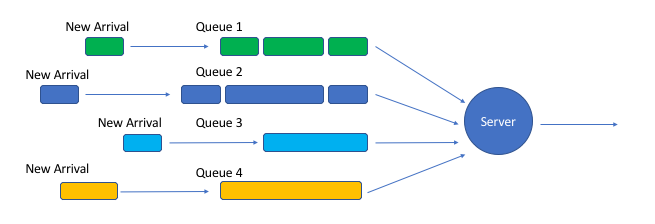
Figure 1.1: Polling System with Four Queues

1.2 Preliminaries

In this subsection we mainly introduce some concepts and terminologies that we use in this paper. Important notations in this paper are provided in Table 1.

Machine Scheduling Problems

Using the notation for one machine scheduling problems [18], we write our problem as $1\mid r_{i},\tau|\sum C_{i}$, where “$1$” refers to the single machine in the system, $r_{i}$ and $\tau$ in the middle field refer to the release date and setup time constraints, and $\sum C_{i}$ in the last field is the completion time objective. In the later part of this paper we will introduce other constraints, which will appear in the middle field, such as $\tau\leq\theta p_{min}$ and $p_{max}\leq\gamma p_{min}$, where $p_{max}=\sup_{i}p_{i}$ is the processing time upper bound and $p_{min}=\inf_{i}p_{i}$ is the processing time lower bound. We say the processing time variation is bounded if $p_{max}\leq\gamma p_{min}$ for constant $\gamma$. If no constraint is specified in this field, it means 1) all jobs are available at time zero, 2) no precedence constraints are imposed, 3) preemption is not allowed, and 4) no setup time exists. In this paper, we assume jobs and setup times are non-resumable and all the policies that we discuss are non-preemptive, unless we specifically state otherwise. Other objectives are $C_{max},$ the maximal completion time or makespan [26] and $\sum w_{i}C_{i},$ the weighted completion time [19].

Online and Offline Problems

A job instance $I$ with $n(I)$ number of jobs is defined as a sequence of jobs with certain arrival times and processing times, i.e., $I=\{(r_{i},p_{i}),1\leq i\leq n(I)\}$. In this work we mainly focus on an online scheduling problem, where $r_{i}$ and $p_{i}$ remain unknown to the server until job $i$ arrives. In contrast to the online problem, the offline problem has entire information for the job instance $I$, i.e., $(r_{1},r_{2},...,r_{n(I)})$ and $(p_{1},p_{2},...,p_{n(I)})$ from time 0. The offline problem is usually of great complexity. The offline version of our online problem, i.e., $1|r_{i},\tau|\sum C_{i}$, is strongly NP-hard since the offline problem with $\tau=0$ is strongly NP-hard [25, 19, 23]. However it is important to note that if preemption is allowed, then Shortest Remaining Processing Time (SRPT) is the optimal policy for $1|r_{i},pmtn|\sum C_{i}$ with $\tau=0$ (see [40]). SRPT is online and polynomial-time solvable. It can be used as a benchmark for online scheduling policies.

Scheduling Policies

A scheduling policy $\pi$ specifies when the server should serve which job. In our paper we mainly focus on online (or non-anticipative) policies [50, 6]. Online policies can be either deterministic or randomized. For example, SRPT is a deterministic policy. A randomized policy may toss a coin before making a decision, and the decision may depend on the outcome of this coin toss [6]. Detailed discussions for randomized algorithms can be found in [41, 10]. In this paper, we focus on deterministic policies.

Notation	Meaning	Notation	Meaning
$r_{i}$	Release date, the time when job $i$ arrives in the system	$p_{i}$	Processing time for job $i$
$p_{max}$	Maximum processing time, $p_{max}=\max_{i}\{p_{i}\}$	$p_{min}$	Minimum processing time, $p_{min}=\min_{i}\{p_{i}\}$
$\tau$	Setup time is $\tau$ for all queues	$I=\{r_{i},p_{i}\}$, for $1\leq i\leq n(I)$	Job instance, set of jobs with information about release date and processing time for all jobs in it
$C^{\pi}(I)$	Total completion time for jobs in instance $I$ under policy $\pi$	$C^{*}(I)$	Total completion time for jobs in instance $I$ under the optimal policy of the offline problem
$C_{i}^{\pi}$	The completion time for job $i$ under policy $\pi$	$n(I)$	Number of jobs in job instance $I$
$\gamma$	Processing time variation, a constant such that $p_{max}\leq\gamma p_{min}$	$\theta$	A constant such that $\tau\leq\theta p_{min}$
$k$	Number of queues in the system	$\kappa=\max\{\frac{k+1}{k}\gamma,k+1\}$	Competitive ratio for cyclic-based and exhaustive-like policies, a constant

Table 1: Notations

Competitive Ratios

A competitive ratio is the ratio between the solution obtained by an online policy and the benchmark. In this paper, the optimal solution to the offline problem is our benchmark. We say the competitive ratio for an online policy is $\rho$ if $\sup_{I}\frac{C^{\pi}(I)}{C^{*}(I)}\leq\rho$, where $C^{\pi}(I)$ is the completion time for job instance $I$ by a deterministic scheduling policy $\pi$ and $C^{*}(I)$ is the optimal completion time of the offline problem. We say a competitive ratio is tight if there exists an instance $I$ such that $\frac{C^{\pi}(I)}{C^{*}(I)}=\rho.$

1.3 Related Work

Single-machine scheduling problems with setup times or costs have been widely studied from various perspectives. A detailed review of the literature can be found in [4, 2, 1, 3, 35]. Other studies considering machine setup can be found in [45, 20, 33, 32, 38]. However, these papers focus on solving the offline problem where all the release times and processing times are revealed at time $0$.

Numerous research papers have shed light on the online single-machine scheduling problems, without considering setup times. Table 2 summarizes the current state of art of competitive-ratio analysis over existing online algorithms for these problems. In addition, a recent paper [30] provides a new method to approximate the competitive ratio for general online algorithms.

Problem	Deterministic		Randomized
	Lower Bounds	Upper Bounds	Lower Bounds	Upper Bounds
$1|r_{i},pmtn|\sum C_{i}$	1	1 [40]	1	1 [40]
$1|r_{i},pmtn|\sum w_{i}C_{i}$	1.073 [13]	1.566 [39]	1.038 [13]	$\frac{4}{3}$ [37]
$1|r_{i}|\sum C_{i}$	2 [21]	2 [21, 29, 34]	$\frac{e}{e-1}$ [41]	$\frac{e}{e-1}$ [10]
$1|r_{i}|$$\sum w_{i}C_{i}$	2 [21]	2 [5]	$\frac{e}{e-1}$ [41]	1.686 [17]
$1|r_{i},\frac{p_{max}}{p_{min}}\leq\gamma|\sum w_{i}C_{i}$	$1+\frac{\sqrt{4\gamma^{2}+1}-1}{2\gamma}$ [44]	$1+\frac{\sqrt{4\gamma^{2}+1}-1}{2\gamma}$ [44]	Unknown	Unknown
$1|r_{i},\frac{p_{max}}{p_{min}}\leq\gamma|\sum C_{i}$	Numerical [43]	$1+\frac{\gamma-1}{1+\sqrt{1+\gamma(\gamma-1)}}$ [43]	Unknown	Unknown

Table 2: Competitive Ratios for single-machine Scheduling Problem without Setup Times (i.e., $\tau=0$)

The online makespan minimization problem for the polling system is considered in [12] and an $\boldsymbol{O}(1)$ policy is proved to exist. However, the competitive ratio provided in [12] is very large. A 3-competitive online policy for the polling system with minimizing the completion time is provided in [52], but only for the case where $k=2$ and jobs are identical. To the best of our knowledge, online policies for general polling systems with setup time consideration have not been well studied.

As we mentioned before, there are articles that study polling systems from a stochastic perspective by assuming job arrivals, service times and setup times are stochastic. Long-run average waiting time, queue length and other metrics of policies are considered for different types of stochastic assumptions [48]. Exact mean waiting time analysis for cyclic routing policies with exhaustive, gated and limited service disciplines for polling system of $M/G/1$ type queues have been provided in [14, 42, 36, 51, 47, 15]. Service disciplines within queues (such as FCFS, SRPT and others) are discussed in [49], but routing disciplines are not discussed. The optimal service policy for the symmetric polling system is provided by [28], where “symmetric” means that queues and jobs are stochastically identical. However, the optimal solution for the general polling system remains unknown [8, 48]. Approximating algorithms for the polling system are very few, and none of those widely-used policies have been shown to work well in general settings.

The contribution of this paper is fourfold: (1) Our work for the first time analyzes polling systems without stochastic assumptions, evaluates policy performance by competitive ratios, provides the conditions for existence of competitive ratios in polling systems, and proves competitive ratios for some well-studied policies such as cyclic exhaustive and gated policy. (2) Our work bridges the queueing and scheduling communities by showing that some widely-used queueing policies also have decent performance in terms of the worst-case performance in online scheduling problems. (3) We provide a lower bound for the competitive ratio for general online policies. (4) We also provide new online policies that balance future uncertainty and utilize known information, which may open up a new research direction that would benefit from revealing information and reducing variability. This paper is organized as follows: in Section 2 we provide some general results for scheduling policies in polling systems; in Section 3 we consider policies which are based on a cyclic routing discipline; in Section 4 we consider policies which are processing-time based; we make concluding remarks in Section 5.

2 General Results

A polling system with zero setup time is the most basic single server system, in which the server only needs to decide when to serve which job, without considering the queue indices. From [40, 16] we know that the optimal online policy is SRPT in this case. The reason is that by doing this, small jobs are quickly processed, thus the number of waiting jobs is reduced. However, it becomes problematic if setup time is non-zero. If a small job arrives at the queue which requires a setup, then processing this small job before other jobs may not be beneficial any more. Deciding which queue to set up and which job to process first thus become challenging in such a polling system.

In the queueing literature, there are many policies which are defined by service disciplines and routing disciplines. The service discipline of each policy determines the time to switch out from a queue and the order to serve jobs. The routing discipline determines the queue to serve next, when the server switches out from a queue. We first introduce some special routing disciplines which are widely studied in the literature.

• Static disciplines: The server visits each queue (could be empty or non-empty) following a static routing table, i.e., a predetermined routing order (see [24, 9]). Cyclic is one of the most basic static routing disciplines, under which the server would visit queues one by one, and returns to the first queue once a cycle has completed.

• Random disciplines: The server visits each queue (could be empty or non-empty) in a random manner (see [24, 11, 22]).

• Purely queue-length based disciplines: An example is Stochastic Largest Queue (SLQ) policy which is defined by [28], where the server under SLQ would choose the largest queue to route to when switching occurs.

• Purely processing-time based disciplines: The next queue to visit could be based on the minimal, maximal, total or average processing time of jobs waiting in the queue. An example is Shortest Processing Time (SPT) policy (see [49]), without considering queue indices.

Interestingly, these disciplines have the same competitive ratio lower bound, of $k$, the number of queues.

Theorem 1.

If an online policy has routing discipline that is: static, random, purely queue-length based, or purely processing-time based, then this online policy cannot have a constant competitive ratio that is smaller than $k$ on $1|r_{i},\tau|\sum C_{i}$.

Proof.

We assume policy $\pi_{1}$ has a routing discipline that is static, random, or processing time based. We give an instance $I$ where there is one job at queue $i=1,...,k-1$ at time 0, and $n$ jobs at queue $k$. Each job has processing time $0$. If $\pi_{1}$ is based on a static discipline, we assume the routing order is from queue 1 to queue $k$; if $\pi_{1}$ is based on random routing discipline, we assume the realization of the random service order is from queue 1 to queue $k;$ if $\pi_{1}$ is purely processing-time based, it treats all queues equally since the minimal, maximal, total, and average processing times for all queues are equal, and we again let the server serve from queue 1 to queue $k$. So the server has to set up $k$ times before reaching queue $k$, and we have

$$C^{\pi_{1}}(I) \geq \tau\left((n+k-1)+(n+k-2)+...+n\right),$$

and

$$C^{*}(I) = \tau\left((n+k-1)+(k-1)+...+1\right).$$

Letting $n\rightarrow\infty$, we have $\frac{C^{\pi_{1}}(I)}{C^{*}(I)}\geq k$.

Now we show the lower bound holds for a policy $\pi_{2}$ that is purely queue-length based. Suppose at time 0, each queue $i=2,...,k$ has one job with processing time 0, and queue 1 has one job with processing time $p.$ Suppose the server under $\pi_{2}$ serves from queue 1 to queue $k,$ which is consistent with queue-length based routing. Then we have

$$C^{\pi_{2}}(I) \geq (k-1)p+p+\frac{k(k+1)}{2}\tau,$$

and

$$C^{*}(I) = p+\frac{k(k+1)}{2}\tau.$$

Letting $p\rightarrow\infty$, we have $\frac{C^{\pi_{2}}(I)}{C^{*}(I)}\geq k.$ ∎

It is important to point out that Theorem 1 provides a competitive ratio bound for policies with some special routing disciplines, but the service discipline for these policies could be arbitrary. We will discuss more about policies that are designed based on service and routing disciplines in Section 3.

To reduce setup frequency, a routing discipline may want to avoid setting up empty queues, although there may be arrivals during setup times. Also, an efficient service discipline may prevent the server from idling when there are unfinished jobs in the system. We thus consider work-conserving policies, under which the server would never idle or set up empty queues when the system is non-empty. The next theorem shows that there exists a constant competitive ratio for all non-preemptive work-conserving policies, under certain conditions.

Theorem 2.

Any non-preemptive work-conserving policy on the polling system with $p_{max}\leq\gamma p_{min}$ and $\tau\leq\theta p_{min}$ is at least $(\gamma+\theta)$-competitive with respect to the optimal solution to the offline problem.

Proof.

Let $I$ be an arbitrary instance, and let $\hat{I}$ be the processing time and setup time augmented instance of $I$ such that all job processing times in $\hat{I}$ are $\hat{p}=p_{max}+\tau\leq(\gamma+\theta)p_{min}$, setup time is 0 and arrival times in $\hat{I}$ are the same as $I$. Note that any non-preemptive work-conserving policy on $\hat{I}$ is optimal since processing times for jobs in $\hat{I}$ are identical, and $\tau=0$. Let $\sigma$ be a non-preemptive work-conserving policy on $I$, and $\hat{\sigma}$ be a policy that works on $\hat{I}$ and serves jobs in the same order as $\sigma$ does in $I$, without idling. Then $\hat{\sigma}$ is work-conserving since $\sigma$ never idles when there are unfinished jobs in system, and therefore $C^{\hat{\sigma}}(\hat{I})=C^{*}(\hat{I})$. We now show $C^{*}(\hat{I})\leq(\gamma+\theta)C^{*}(I).$ Let $S_{i}^{*}$ and $C_{i}^{*}$ be the starting and completion times of job $i$ in $I$ under the optimal solution. Let $\delta$ be a schedule that works on $\hat{I}$ and finishes each job $i$ at time $(\gamma+\theta)C_{i}^{*}$, we then have $C^{\delta}(\hat{I})=(\gamma+\theta)C^{*}(I).$ We now show that $\delta$ is a feasible schedule on $\hat{I}.$ Notice that schedule $\delta$ starts serving job $i$ in $\hat{I}$ at time $\hat{S}_{i}^{\delta}=(\gamma+\theta)C_{i}^{*}-\hat{p}=(\gamma+\theta)(S_{i}^{*}+p_{i})-\hat{p}\geq(\gamma+\theta)S_{i}^{*}\geq r_{i}$. Since $S_{i}^{*}\geq C_{i-1}^{*},$ we also have $(\gamma+\theta)S_{i}^{*}\geq(\gamma+\theta)C_{i-1}^{*}$. Therefore $\hat{S}_{i}^{\delta}\geq\max\{r_{i},(\gamma+\theta)C_{i-1}^{*}\},$ by induction we can show that $\delta$ is a feasible schedule on $\hat{I}$. In summary, we have

$$C^{\sigma}(I)\leq C^{\hat{\sigma}}(\hat{I})=C^{*}(\hat{I})\leq C^{\delta}(\hat{I})=(\gamma+\theta)C^{*}(I).$$

∎

Note that Theorem 2 holds only when $p_{max}\leq\gamma p_{min}$ and $\tau\leq\theta p_{min}$. If either inequality does not hold, we may need other scheduling policies to achieve constant competitive ratios, which we will discuss in Section 3 and Section 4.

3 Scheduling Policies with Cyclic Routing

In this section we focus on scheduling policies with static routing disciplines. While these policies are easy to implement, they cannot, e.g., prioritize small jobs. To characterize the influence made by job processing time variation, in this section we assume $p_{max}\leq\gamma p_{min}$. When $\gamma$ is small, all jobs have similar processing times. Unlike in [43] where $p_{min}$ is assumed to be non-zero, here we also allow $p_{min}=p_{max}=0$, for which we define $\gamma$ to be 1.

In Theorem 1 we have shown that the competitive ratio for a policy with a static or random routing discipline is at least $k$, for the system $1|r_{i},\tau|\sum C_{i}$. Even with additional assumption $p_{max}\leq\gamma p_{min}$, we show in the following theorem that the competitive ratio for a policy with a static or random routing discipline is still lower bounded by $k$. In this case, cyclic routing is the only static discipline that can achieve this lower bound.

Theorem 3.

No online policy with a static or random routing discipline can guarantee a competitive ratio smaller than $k$ for $1|r_{i},\tau,p_{max}\leq\gamma p_{min}|\sum C_{i}$, and cyclic routing is the only static routing discipline that can achieve this lower bound.

Proof.

Since $1|r_{i},\tau,p_{i}=1|\sum C_{i}$ is a special case of $1|r_{i},\tau,p_{max}\leq\gamma p_{min}|\sum C_{i}$, we here only need to show the lower bound $k$ holds for $1|r_{i},\tau,p_{i}=1|\sum C_{i}$. For an arbitrary policy that follows a static routing discipline, we suppose the server starts from queue 1, and queue $k$ is the last one visited. Before visiting queue $k$ for the first time, the server visits queue $i$ for $v_{i}$ times $(1\leq i\leq k-1)$. We construct a special job instance $I$ by assuming that there is one job arriving at each queue $i$ every time the server visits queue $i$ for $i=1,...,k-1$. Also we suppose there are $n_{k}$ jobs at queue $k$ at time 0 for a large $n_{k}$, and say they form a batch $b_{k}$. If we let $g(b_{k})=\frac{n_{k}(n_{k}+1)}{2},$ then we have

$$C^{\pi}(I\cup b_{k}) \geq C^{\pi}(I)+n_{k}\tau(\sum_{i=1}^{k-1}v_{i}+1)+g(b_{k}),$$

$$C^{*}(I\cup b_{k}) \leq C^{\pi}(I)+n_{k}\tau+g(b_{k})+n(I)(n_{k}+\tau),$$

and $\frac{C^{\pi}(I\cup b_{k})}{C^{*}(I\cup b_{k})}\geq\sum_{i=1}^{k-1}v_{i}+1$ if we let $\tau=(n_{k})^{2}$ and $n_{k}\rightarrow\infty$. Since for any static or random routing discipline we can construct a job instance like this, to achieve the smallest ratio $\sum_{i=1}^{k-1}v_{i}+1$, we need $v_{i}=1$ for $i=1,...,k-1$. Therefore $\frac{C^{\pi}(I\cup b_{k})}{C^{*}(I\cup b_{k})}\geq k$ and only cyclic routing can achieve this lower bound. ∎

Theorem 3 shows the advantage of cyclic routing over the other static and random routing disciplines for $1\mid r_{i},\tau,p_{max}\leq\gamma p_{min}\mid\sum C_{i}$. We now focus our discussion on service disciplines at each queue assuming cyclic routing. We first discuss a service discipline called exhaustive, under which the server serves all the jobs in a queue before switching out. We show that the exhaustive service has a competitive advantage over the other disciplines when all job processing times are identical.

Proposition 4.

For the polling system $1|r_{i},\tau,p_{min}=p_{max}|\sum C_{i}$, there always exists an exhaustive discipline whose competitive ratio is at least as small as a non-exhaustive discipline.

Proof.

The case where $p_{i}=0$ is trivial. Now we let $p_{i}=1$ with appropriate units. Since preemption is not allowed and all the jobs are identical, the server only needs to decide when to switch out and which queue to set up next. If there are jobs in the queue that the server is currently serving, there are two options for the server: to continue serving the next job in this queue, or to switch to a queue and later come back to this queue again. If at time 0 the server is at queue 1 and there is an unfinished job in queue 1, then the server has to come back after it switches out. Suppose under a non-exhaustive policy $\pi^{{}^{\prime}}$, the server chooses to switch to some queue(s) and come back to queue 1 at time $T$. Say the server serves instance $I^{{}^{\prime}}$ during this period $T$. Suppose there is an adversary policy which has the same instance at time 0, and this policy chooses to serve one more job in queue 1, and then follows all decisions that policy $\pi^{{}^{\prime}}$ has made (including waiting). Note that every decision policy $\pi^{{}^{\prime}}$ made is available to the adversary policy because the adversary policy serves one more job before leaving queue 1. The total completion time under $\pi^{{}^{\prime}}$ is $C^{\pi^{{}^{\prime}}}=1+T+C(I^{{}^{\prime}})$, and the completion time achieved by the adversary is $C^{ad}=1+C(I^{{}^{\prime}})+n(I^{{}^{\prime}})$, where $C(I^{{}^{\prime}})$ is the completion time of instance $I$ served by policy $\pi^{{}^{\prime}}$ during $(0,T]$. We then have $C^{ad}-C^{\pi^{{}^{\prime}}}\leq n(I^{{}^{\prime}})-T\leq 0$. Notice that the makespan of these two schemes are the same (including the final setup time of queue 1 for the adversary). Then by induction, we can show that there always exists an exhaustive discipline that can achieve a smaller total completion time than a non-exhaustive one. ∎

Theorem 3 and Proposition 4 motivate us to consider scheduling policies with cyclic routing and exhaustive service. Define a set of policies $\Pi_{1}$ as those policies under which the server 1) serves queues in a cyclic way and skips empty queues when switching, 2) serves each queue exhaustively, 3) stays in queue $i$ for at most $n_{i}^{w}p_{max}$ amount of time before switching out, where $n_{i}^{w}$ is the number of jobs processed in the server’s $w^{th}$ visit to queue $i$, and 4) idles at the last queue that it served if all queues are empty. Note that after serving all the jobs in queue $i$, the server is allowed to wait in queue $i$ for some extra time to receive more arrivals. If a new arrival occurs at queue $i$ during the time that the server is waiting, then $n_{i}^{w}\leftarrow n_{i}^{w}+1$ and the server can process this job at any time before it switches out, as long as the server does not stay in the queue for time longer than the updated $n_{i}^{w}p_{max}$. If during the $w^{th}$ visit to queue $i$, the processing time for each job in the queue is $p_{max}$, then the server will switch out immediately once a queue is exhausted. Also note that we do not specify the service order of jobs for policies in $\Pi_{1}$.

Notice that the policies in $\Pi_{1}$ does not set up empty queues, so the routing discipline for these policies needs to utilize the queue information. We next consider policies which do not require any queue information, so the server under these policies would set up each queue even if the queue is empty before setup is initiated. Let the set of policies $\Pi_{2}$ be defined as for $\Pi_{1}$ except that the server sets up regardless of whether the queue is empty or not. It is important to point out that the policy without waiting (just exhaustively serving) belongs to $\Pi_{2}$, and the long-run average waiting time and queue length under this policy have been extensively studied for $M/G/1$ type queues [14, 42, 36, 51].

Another widely studied service discipline is called gated. Under a gated discipline, the server only serves the jobs that have arrived in the queue before the server finishes setting up the queue, and jobs that arrive after that time will be left to the next cycle of service. We now let $\Pi_{3}$ be the set of policies with cyclic routing with skipping the empty queues, and that serves each queue with a gated discipline. Similar to policy set $\Pi_{1},$ we do not specify the service order for $\Pi_{3}$ either. Once the server has set up queue $i$, the number of jobs at that time, $n_{i}^{w}$, will be served during this visit. We also allow the server to wait after clearing a queue under $\Pi_{3}$, and the maximal time for staying in queue $i$ in the $w^{th}$ visit is bounded by $n_{i}^{w}p_{max}$. Similarly, we can have a policy set $\Pi_{4}$ in which policies are cyclic and gated, without skipping empty queues when switching. We do not provide the detailed description of $\Pi_{4}$ here since it is similar to policy set $\Pi_{3}.$ The long-run average queue length and waiting time under the gated discipline for $M/G/1$ type queues are also provided in [42, 51], if the server does not skip empty queues when switching.

So far we have introduced four policy sets, and we let $\Pi_{r}=\cup_{i=1}^{4}\Pi_{i}.$ In the next theorem we show that all the policies in $\Pi_{r}$ have the same competitive ratio for problem $1\mid r_{i},\tau,p_{max}\leq\gamma p_{min}\mid\sum C_{i}$.

Theorem 5.

Any policy $e\in\Pi_{r}$ has the competitive ratio $\kappa=\max\{\frac{k+1}{k}\gamma,k+1\}$ for the polling system $1\mid r_{i},\tau,p_{max}\leq\gamma p_{min}\mid\sum C_{i}$. When $\gamma\leq k$, for arbitrary $\epsilon>0$, there is an instance $I$ such that $\frac{C^{e}(I)}{C^{*}(I)}>\kappa-\epsilon=k+1-\epsilon$.

Proof.

The detailed proof in given in the Appendix A. ∎

From Theorem 3 we know that the competitive ratio based on static or random routing is at least $k$, and Theorem 5 shows that any policy from $\Pi_{r}$ has an approximately tight competitive ratio $k+1$ if $\gamma\leq k$. This indicates that policies from $\Pi_{r}$ are nearly optimal among all the policies that are based on static or random routing disciplines. It is also important to point out that although gated service disciplines are different from exhaustive disciplines, one can also regard a gated discipline as an exhaustive-like discipline, as the server under a gated discipline would exhaust the jobs that have arrived in the previous cycle. The policies in $\Pi_{r}$ have a constant competitive ratio for $1|r_{i},\tau,p_{max}\leq\gamma p_{min}|\sum C_{i}$ because of this exhaustive-like service discipline, since the server under a policy from $\Pi_{r}$ would serve as many jobs as possible before switching out. Some other cyclic policies without using an exhaustive-like service may not have constant competitive ratios for $1|r_{i},\tau,p_{max}\leq\gamma p_{min}|\sum C_{i}$. We now consider a policy called the $l$-limited policy. This policy is also based on the cyclic routing. However, the server under the $l$-limited policy only serves at most $l$ jobs during each visit to a queue. A detailed description for this policy and the long-run average waiting time under this policy for $M/G/1$ type queues can be found in [42, 15, 47]. Interestingly, as we shall show in Proposition 6, no constant competitive ratio is guaranteed by the $l$-limited policy, regardless whether the server skips empty queues or not.

Proposition 6.

The $l$-limited policy ($l<\infty$, with or without skipping empty queues) does not have a constant competitive ratio for $1\mid r_{i},\tau,p_{max}\leq\gamma p_{min}\mid\sum C_{i}$.

Proof.

We prove this result by giving a special instance $I$. Suppose there are $(l*n)$ number of jobs $(l,n\in\mathbf{Z_{+})}$ at every queue at time $0$, and each job has processing time $p=1$. At each queue the server sets up and serves $l$ jobs, and this is repeated $n$ times. Let $C^{l}(I)$ be the total completion time for the l-limited policy (either with or without skipping empty queues), we have

$$\frac{C^{l}(I)}{C^{*}(I)} = \frac{\frac{knl(knl+1)}{2}+\tau l\frac{kn(kn+1)}{2}}{\frac{knl(knl+1)}{2}+\tau nl\frac{k(k+1)}{2}}.$$

If we let $\tau=(n)^{2}$ and $n\rightarrow\infty$, then $\frac{C^{l}(I)}{C^{*}(I)}\rightarrow\infty$. ∎

Proposition 6 shows that the $l$-limited policy, which does not belong to $\Pi_{r},$ does not have a constant competitive ratio for $1\mid r_{i},\tau,p_{max}\leq\gamma p_{min}\mid\sum C_{i}$. Theorem 5 and Proposition 6 show the advantage of exhaustive-like service disciplines. However, policies in $\Pi_{r}$ also have their limitations. We next show that policies in $\Pi_{r}$ do not have constant competitive ratios if $p_{min}=0<p_{max}$ (so $\gamma$ is infinity).

Theorem 7.

Policies in $\Pi_{r}$ do not guarantee constant competitive ratios for $1|r_{i},\tau|\sum C_{i}$.

Proof.

We prove the theorem by giving a special job instance $I$. We assume $p_{min}=0$ and $p_{max}=p$ so that $\gamma=\infty$. Suppose at time $0$ each of queue $i=2,...,k$ has one job with processing time $p$ and queue 1 has no job. At time $\tau+\epsilon$ there are $n$ jobs arriving at queue 1, with each having processing time $0$. For any policy $\pi\in\Pi_{r}$, the server would either setup queue 1 at time 0 then switch to queue 2 at time $\tau$, or setup queue $2$ at time 0. In either of the cases the server will be back to queue 1 when queue $k$ is served in the first cycle. Then we have

$$C^{\pi}(I) \geq \frac{k(k-1)}{2}p+n(k-1)p+\tau\left((n+k-1)+(n+k-2)+...+n\right),$$

and

$$C^{*}(I) = \frac{k(k-1)}{2}p+\tau\left((n+k-1)+(k-1)+...+1\right)+\epsilon(n+k-1).$$

Letting $p=(n)^{2}$ and $n\rightarrow\infty$, we have $\frac{C^{\pi}(I)}{C^{*}(I)}\rightarrow\infty.$ ∎

Theorem 7 shows the limitation of $\Pi_{r}$ when the condition $p_{max}\leq\gamma p_{min}$ is not satisfied. Although the server under $\Pi_{r}$ can serve the jobs within each queue following SPT (see[49]) to achieve a smaller expected waiting time, the competitive ratio remains $\kappa$. When the condition $p_{max}\leq\gamma p_{min}$ no longer holds for finite $\gamma$, one may need policies that utilize the job processing time information to achieve a constant competitive ratio. In the next section we will introduce some processing-time based policies when $p_{max}\leq\gamma p_{min}$ does not hold.

4 Scheduling Policies Based on Job Processing Times

In this section we mainly discuss policies in which service and routing disciplines are based on job processing times. Service and routing disciplines for these policies are based on job processing times only. To better characterize the competitive ratio for these policies, in this section we assume the setup time $\tau$ is bounded by a ratio of the minimal processing time, that is $\tau\leq\theta p_{min}.$ If $\tau=p_{min}=0,$ we let $\theta=1.$ This setting in the 3D printing example corresponds to the scenario where jobs of a different color need to be printed, and the time to set up a new ink is bounded by a constant factor of the minimum possible processing time. Using the standard notation for scheduling problems (see [18]), we denote this polling problem as $1|r_{i},\tau\leq\theta p_{min}|\sum C_{i}$. Notice that when the setup time is small, i.e., $\theta$ is small, switching may not be the major contributor to the completion time. Thus these processing-time based policies may be efficient when $\theta$ is small.

We first introduce a benchmark for deriving the competitive ratio of our policies. Usually the competitive ratio $\rho$ is defined by $\sup_{I}\frac{C^{\pi}(I)}{C^{*}(I)}\leq\rho$ where $C^{*}(I)$ is the completion time for $I$ in the offline optimal solution. The offline problem is strongly NP-hard. To non-rigorously show the NP-hardness, we know that if no preemption is allowed, even the easier problem $1|r_{i}|\sum C_{i}$ (without setup time) is strongly NP-hard [25, 19, 23]. In this section we use a lower bound of the optimal solution as the benchmark. To get a lower bound for the optimal solution, we introduce the idea of setup time reduced instance. If instance $I$ is an arbitrary job instance, then the setup time reduced instance of $I$, say $\utilde{I}$, is an instance that has the same jobs (same arrival times and same processing times) as $I$, but has no setup times. The optimal scheduling policy for $\utilde{I}$ to minimize total completion times is SRPT [40]. This scheduling policy is also online, which is handy for other online policies to emulate. The completion time of instance $\utilde{I}$ under SRPT is denoted by $C^{p}(\utilde{I})$. Since setup time does not exist in $\utilde{I}$, we have $C^{p}(\utilde{I})\leq C^{*}(I)$. In this section, we only consider non-preemptive policies, but using SRPT as the benchmark. When preemption is not allowed, One Machine (OM) policy is known to be the optimal online scheduling policy for $\utilde{I}$ [34]. We now apply OM on instance $I$ and prove its competitive ratio for polling systems. The description of the OM policy is provided in Algorithm 1. Note that under OM, a job in $I$ can only be scheduled (started) once it has been completed by SRPT on $\utilde{I}$. The competitive ratio of OM is provided in Theorem 8.

1. Simulate SRPT policy on the setup time reduced instance $\utilde{I}$.

2. Schedule the jobs non-preemptively in the order of completion time of jobs by SRPT on $\utilde{I}$.

Algorithm 1 One Machine Scheduling (OM)

Theorem 8.

OM is a $(2+\theta)$-competitive online algorithm for the polling system $1|r_{i},\tau\leq\theta p_{min}|\sum C_{i}$. The competitive ratio is tight when using SRPT on the reduced instance as the benchmark.

Proof.

Let the completion time of the $j^{th}$ job under OM scheduling be $C_{j}^{o}$, and the completion time of the $j^{th}$ job completed under SRPT be $C_{j}^{p}$. Since job $j$ is also the $j^{th}$ job that completes service under SRPT, we have $\sum_{i=1}^{j}p_{i}\leq C_{j}^{p}$. Then we have $C_{j}^{o}\leq C_{j}^{p}+\sum_{i:C_{i}^{p}\leq C_{j}^{p}}p_{i}+j\tau\leq(1+\theta)C_{j}^{p}+\sum_{i=1}^{j}p_{i}\leq(2+\theta)C_{j}^{p}$. Since $C^{p}(\utilde{I})\leq C^{*}(I),$ we get $\sum C_{i}^{o}\leq(2+\theta)\sum C_{i}^{p}\leq(2+\theta)\sum C_{i}^{*}$. The competitive ratio is tight when there is only one job in the instance $I$ which is available at time $0$. Suppose this job has processing time $1$. Then $C^{p}(I)=1$, and $C^{o}(I)=1+(1+\theta)=2+\theta$. ∎

The OM algorithm is intuitive, easy to apply and polynomial-time solvable. Despite its simplicity, we may find it inefficient since setup times are ignored. Although each unnecessary switch only brings a small amount of delay if $\theta$ is small, we may still want to avoid switching too often. Thus we provide another policy that is based on OM, under which the server will avoid unnecessary setups. We call it the Modified One Machine (MOM) policy, with description in Algorithm 2. Under MOM, we will 1) regard the completion time of each job under SRPT on $\utilde{I}$ as the new “arrival” time, 2) modify the processing time for job $i$ as $p_{i}+\tau$ if it is not located in the queue that the server is serving, and 3) process the job with smallest modified processing time. After completing a job, the processing time for all the jobs in the system is modified again, and the same mechanism is repeated. Under MOM, the server will prefer the jobs from the queue that it is currently serving, thus avoiding frequent switching. We denote the completion time of job $i$ in $I$ by MOM as $C_{i}^{g}$.

1:Instance $I$

2:Denote the queue that the server is serving as $queue_{server}$

3:while $I$ has not been fully processed do

4:     Simulate SRPT on $\utilde{I}$. Regard the departure time of the $i^{th}$ job in SRPT as the $i^{th}$ arrival time in MOM.

5:     if $i^{th}$ arrival is at $queue_{server}$ then

6:         $\tilde{p}_{i}={p_{i}}$

7:     else

8:         $\tilde{p}_{i}={p_{i}+\tau}$

9:     end if

10:     Schedule the job with smallest $\tilde{p}_{i}$

11:end while

12:return Total completion time $C^{g}(I)$

Algorithm 2 Modified One Machine Scheduling (MOM)

Theorem 9.

MOM is a $(2+\theta)$-competitive online algorithm for $1|r_{i},\tau\leq\theta p_{min}|\sum C_{i}$. The competitive ratio is tight when using SRPT on the reduced instance as the benchmark.

Proof.

Note both MOM and OM simulate SRPT on $\utilde{I}$ and schedule job $i$ only after job $i$ has been processed in SRPT. So we can regard OM as FCFS for a job instance with arrival times {$C_{i}^{p}$,$i=1,2,...$}, while MOM serves the job with the smallest modified processing first in this instance with the same arrival times. We have $C_{j}^{g}\leq C_{j}^{p}+\sum_{i=1}^{j}\tilde{p_{i}}$, where $\tilde{p_{i}}$ is the modified processing time of job $i$. Since MOM schedules the available jobs in the descending order of $\tilde{p}_{i}$, we have $C_{j}^{g}\leq C_{j}^{p}+\sum_{i=1}^{j}\tilde{p_{i}}\leq C_{j}^{p}+\sum_{i:C_{i}^{p}\leq C_{j}^{p}}(p_{i}+\tau)\leq(2+\theta)C_{j}^{p}$. We give the same example as in Theorem 8 to show the tightness of competitive ratio: Suppose there is only one job with $p=1$ in instance $I$, available at time $0$. Then $C^{p}(I)=1$, and $C^{g}(I)=1+(1+\theta)=2+\theta$. ∎

Though MOM avoids some switching, OM and MOM have the same competitive ratio when using SRPT on reduced instance as the benchmark.

Next we show the lower bound for competitive ratios of the problem $1|r_{i},\tau=\theta p_{min}|\sum C_{i}$. Notice this is a special case for the problem $1|r_{i},\tau\leq\theta p_{min}|\sum C_{i}$.

Theorem 10.

If $\tau=\theta p_{min}$ and $\theta\geq 0$, then there is no online algorithm whose competitive ratio is smaller than $\theta+1$, using SRPT on the reduced instance as the benchmark.

Proof.

If there is one job with processing time $p_{min}$ in the system, we have $\frac{C^{\pi}(I)}{C^{p}(I)}\geq\frac{(1+\theta)p_{min}}{p_{min}}=1+\theta$. If $\tau=p_{min}=0$ (so $\theta=1$), then the lower bounded ratio is $\theta+1=2$ as provided in [21]. ∎

A natural question is whether this lower bound is the best lower bound that one can have. The answer remains open. There could be either an online policy whose competitive ratio is exactly equal to this lower bound, or a larger lower bound which is closer to the ratio $(2+\theta)$.

So far we have shown the existence of constant competitive ratios under different assumptions for polling systems as summarized in Table 3. We find that when either $p_{max}\leq\gamma p_{min}$ or $\tau\leq\theta p_{min}$ holds, we can have constant competitive ratios. In fact, in many practical scenarios either the processing time is bounded or the setup time is bounded or both. Also, when $p_{max}\leq\gamma p_{min}$ and $\tau\leq\theta p_{min}$ both hold, any work-conserving policies, as well as policies from $\Pi_{r}$, OM, and MOM all have constant competitive ratios. When processing time variation is relatively small compared with the setup time, i.e., $\gamma$ is small and $\theta$ is large, then policies from $\Pi_{r}$ can have a smaller competitive ratio than OM or MOM. On the other hand, when $\theta$ is small while $\gamma$ or $k$ is large, using OM or MOM may be more efficient as setup times do not contribute much to the total completion time. When $1\leq\gamma<2$, a work-conserving policy outperforms OM and MOM, and it also outperforms policies from $\Pi_{r}$ if $\theta<\frac{1}{k}\gamma$ and $\gamma\geq k$.

Assumption	Competitive Ratio
$p_{max}\leq\gamma p_{min}$, $\tau\leq\theta p_{min}$	$\min\{2+\theta,\gamma+\theta,\max\{\frac{k+1}{k}\gamma,k+1)\}\}$
$\tau\leq\theta p_{min}$	$2+\theta$
$p_{max}\leq\gamma p_{min}$	$\max\{\frac{k+1}{k}\gamma,k+1\}$
Unbounded Processing Time and Setup Time	$\geq 2$

Table 3: Competitive Ratios for Different Cases

5 Concluding Remarks and Future Work

In this paper we consider scheduling policies in the polling system without stochastic assumptions. Conditions for the existence of constant competitive ratios are discussed and competitive ratios for several well-studied polling system scheduling policies are provided. Specifically, we show that for $1\mid r_{i},\tau,p_{max}\leq\gamma p_{min}\mid\sum C_{i}$ system, an online policy needs to have a cyclic routing discipline and exhaustive-like service discipline to achieve a constant competitive ratio. We provide a policy set $\Pi_{r}$ such that every policy from $\Pi_{r}$ has a constant competitive ratio $\kappa$ for problem $1\mid r_{i},\tau,p_{max}\leq\gamma p_{min}\mid\sum C_{i}$. We further provide processing-time based policies which have constant competitive ratios in system $1\mid r_{i},\tau\leq\theta p_{min}\mid\sum C_{i}$. We show that if the routing discipline for an online policy is static, random, purely queue-length based, or purely processing-time based, then the competitive ratio of this policy cannot be smaller than $k$. However, it remains unknown whether there exists an online policy with a constant competitive ratio for the problem $1\mid r_{i},\tau\mid\sum C_{i}$ without any bounding conditions for processing times and setup times.

Appendix A Proof for Theorem 5 in the Main Paper

In this section we mainly provide the proof for Theorem 5 of our paper. We first introduce a fact that will be useful later in our proof.

Fact 11.

For positive numbers $\{a_{i},b_{i}\}_{i=1}^{n}$, we have $\frac{\sum_{i=1}^{n}a_{i}}{\sum_{i=1}^{n}b_{i}}\leq\max_{i=1}^{n}\{\frac{a_{i}}{b_{i}}\}.$

Proof.

Without loss of generality, assume $\frac{a_{n}}{b_{n}}=\max_{i=1}^{n}\{\frac{a_{i}}{b_{i}}\},$ then for any $i$ we have $\frac{a_{n}}{b_{n}}\geq\frac{a_{i}}{b_{i}}$, thus $a_{n}b_{i}\geq a_{i}b_{n}$ holds for all $i=1,...,n$. Since $\frac{a_{n}}{b_{n}}-\frac{\sum_{i=1}^{n}a_{i}}{\sum_{i=1}^{n}b_{i}}=\frac{a_{n}\sum_{i=1}^{n}b_{i}-b_{n}\sum_{i=1}^{n}a_{i}}{b_{n}(\sum_{i=1}^{n}b_{i})}=\frac{\sum_{i=1}^{n}(a_{n}b_{i}-a_{i}b_{n})}{b_{n}(\sum_{i=1}^{n}b_{i})}\geq 0$, we have $\frac{\sum_{i=1}^{n}a_{i}}{\sum_{i=1}^{n}b_{i}}\leq\frac{a_{n}}{b_{n}}=\max_{i=1}^{n}\{\frac{a_{i}}{b_{i}}\}$. ∎

In Theorem 5 we want to show $\sup_{I}\frac{C^{e}(I)}{C^{*}(I)}\leq\rho$ for some constant $\rho.$ However, by Fact 11 we only need to show that this inequality holds for the instance processed in each busy period of the server under an online policy $e\in\Pi_{1}$. Here we first introduce the concept of busy periods under the online policy. If there is at least one job in the system, we say the system is busy, otherwise it is empty. When the system is empty, the server is not serving under the online policy. The status of the system under the online policy can be described as a busy period following an empty period, and then following by a busy period, and so on. There are two types of busy periods that we are interested in. A Type I busy period (denoted as I-B) is the busy period in which the server resumes work without setting up. This is because the server was idling at the last queue it served (say queue $i$) after the previous busy period, and the first arrival in the new busy period also occurs at queue $i$. A Type II busy period (denote as II-B) is the busy period in which the server resumes work with a setup, because the new arrival occurs at a queue different from the queue where the server was idling. Note that the total job instance may be processed by the online policy in multiple busy periods, and in the proof we only consider the subset of this job instance that is processed in a certain busy period, which we call busy period instance. Also note that the very first busy period must be a II-B, since the server has to set up a queue before processing at the very beginning.

Without loss of generality, we say a cycle (round) starts when the server under the online policy visits queue 1 and ends when it visits queue 1 the next time. If at some time point a queue, say queue $i$, is empty and skipped by the server, we still say that queue $i$ has been visited in this cycle, with setup time 0. We define the job instance served by the server in its $w^{th}$ visit to queue as $b_{i}^{w}$ (for $i=1,...,k$), and we call each $b_{i}^{w}$ a batch. Batch $b_{i}^{w}$ is a subset of job instance $I$. In each cycle, there are $k$ batches served by the online policy, and some, but not all may be empty (if all of them are empty then the system is empty and the server would idle at queue 1). We let $I^{w}=\cup_{i=1}^{k}b_{i}^{w}$. For each batch $b_{i}^{w}$ with the number of jobs $n(b_{i}^{w})=n_{i}^{w}$, $S_{i}^{w}$ is the earliest time when a job from $b_{i}^{w}$ starts being processed under the online policy, and $R_{i}^{w}$ is the earliest release date (arrival time) over all jobs from batch $b_{i}^{w}$. Notice that $R_{i}^{w}\leq S_{i}^{w}$. Each batch $b_{i}^{w}$ may be processed by the optimal offline policy in a different way from the online policy. Suppose $E_{i}^{w*}$ is the earliest time when a job in batch $b_{i}^{w}$ starts service under the optimal offline policy. Note $E_{i}^{w*}$ may differ from $S_{i}^{w}$. Before time $S_{i}^{w}$, we know all the batches $(\cup_{j=1}^{w-1}I^{j})\cup(\cup_{l=1}^{i-1}b_{l}^{w})$ have been served by the online policy. However in the optimal offline policy, only some jobs from these batches have been served, and some other jobs from other cycles of the online policy may have already been served. We suppose $q_{i}^{w}$ number of jobs in $(\cup_{j=1}^{w-1}I^{j})\cup(\cup_{l=1}^{i-1}b_{l}^{w})$ have been served by the optimal offline policy before time $E_{i}^{w*}$. We define $E_{i}^{w}$ as the earliest time when the truncated optimal offline policy starts to serve batch $b_{i}^{w}$, where the idea of truncated optimal offline policy will be defined later. We let $C^{e}(I)$ be the cumulative completion times of all jobs in job instance $I$ under online policy $e\in\Pi_{1}$, and $C^{*}(I)$ be the cumulative completion times of all jobs in $I$ under the offline optimal policy. For convenience, we let $g(I)=\frac{n(I)\left(n(I)+1\right)}{2}$ for job instance $I$, which is the sum of arithmetic sequence from 1 to $n(I)$. Also, $g(I)$ can be regarded as the completion time of $I$ when 1) all the jobs are available at time $0$, 2) each of them has processing time $1$, and 3) no setup time is considered. All the notations are summarized in Table 4 of this document. Before going to the proof of Theorem 5, we first provide an example to show how the total completion time is characterized.

Example 12.

Suppose there is a job instance $I$ with $n(I)=n_{1}+n_{2}$ jobs which arrive at time $R$. Each of the job has processing time $1$. Under some policy $\pi$, suppose the server starts to process the first $n_{1}$ jobs, and idles for time $W$, and then processes the rest of $n_{2}$ jobs without idling. The total completion time for $I$ is given by

$$C^{\pi}(I) = (R+1)+(R+2)+...+(R+n_{1})+(R+n_{1}+W+1)+(R+n_{1}+W+2)+...+(R+n_{1}+W+n_{2})$$

$$= (n_{1}+n_{2})R+n_{2}W+g(I).$$

Notice the completion time of $I$ is made up of three components. The first component $(n_{1}+n_{2})R$ is because all the jobs in $I$ arrive at time $R$. The second term $n_{2}W$ is because the remaining $n_{2}$ jobs wait for another $W$ amount of time. The third term $g(I)$ is the pure completion time if we process jobs one by one without idling.

Notice that the optimal policy may not always be work-conserving (i.e., never idles when there are jobs in the system). The optimal policy may wait at some queue in order to receive more jobs which will arrive in the future. The truncated optimal solution (of a busy period instance $I$) is defined by the completion time for the optimal offline problem minus the additional completion time caused by idling, which is shown in Figure A.1. There is a waiting (idling) period $W$ between $b_{1}^{1}$ and $b_{1}^{2}$ in Figure A.1. The truncated optimal solution is given by $C^{*}(b_{1}^{1}\cup b_{1}^{2}\cup b_{2}^{1}\cup b_{3}^{1})-W(n_{1}^{2}+n_{2}^{1}+n_{3}^{1})$. We use $C^{t}(I)$ to denote the total completion time for a busy period instance $I$ under the truncated optimal schedule. Note that this truncated optimal solution is only for an instance $I$ served by the online policy during a specific busy period, so the earliest start time of service of this truncated optimal policy cannot be earlier than the earliest arrival time of $I$. Also note that the truncated optimal solution is always a lower bound for the real optimal solution.

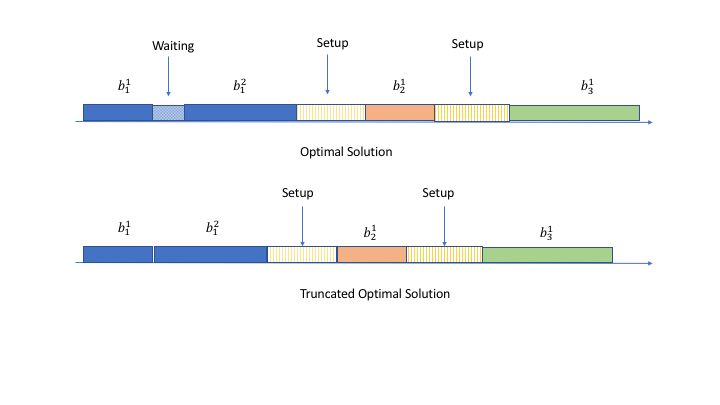
Figure A.1: Truncated Optimal Solution

Lemma 13.

Suppose $I$ is a job instance served in a busy period by the online policy, $b$ is a batch in some cycle for the offline problem and $p_{min}=1$, then $C^{t}(I\cup b)\geq C^{t}(I)+g(b)+En(b)+n(b)(n(I)-q),$ where $E$ is the time when the server starts serving batch $b$ in the truncated optimal solution, and $q$ is the number of jobs in $I$ that are served before time $E$.

Proof.

We suppose the optimal solution is given, and now we consider the total completion time of $I\cup b$ under truncated optimal solution. If all the jobs from $b$ are served after $I$ in the optimal solution, then we have $C^{t}(I\cup b)\geq C^{t}(I)+g(b)+En(b)$. If not, we let $\delta(b)=C^{t}(I\cup b)-C^{t}(I)$ be the additional completion time incurred by inserting $b$ into $I$. Notice that $\delta(b)$ is minimized when all jobs in $b$ has $p_{min}=1$. If we can show that $\delta(b)\geq g(b)+En(b)+n(b)(n(I)-q)$ with every job in $b$ having $p_{min}=1$, we can then prove the lemma. So we assume here that every job in $b$ has $p_{min}=1$. Since the earliest time to process batch $b$ in the truncated optimal solution is $E,$ if we combine all jobs in $b$ altogether and serve them in one batch from time $E$ to time $E+n(b)$, then $\delta(b)$ is again minimized since all the jobs in $b$ have the smallest processing time. So in the following we show that by inserting batch $b$ at time $E,$ the additional completion time incurred is at least $g(b)+En(b)+n(b)(n(I)-q).$ By inserting batch $b$ into $I$ from time $E$ to $E+n(b)$, some jobs from $I$ served after $E$ in the original truncated optimal solution (with total number $(n(I)-q)$) are moved after batch $b$, resulting an increase of delay $n(b)(n(I)-q)$ for these jobs. Besides, inserting a batch $b$ at time $E$ increases the total completion time by $g(b)+En(b)$. ∎

Lemma 13 is illustrated in Figure A.2. The first schedule in Figure A.2 is the truncated optimal for the batch $b_{1}^{1}\cup b_{2}^{1}\cup b_{3}^{1}$. The second schedule is the truncated optimal schedule for $b_{1}^{1}\cup b_{2}^{1}\cup b_{3}^{1}\cup b$, where $b$ is separated into two parts. If all jobs in $b$ have processing time $p_{min}=1$, it is always beneficial to schedule all jobs of $b$ in the same batch, which is shown as the third schedule in Figure A.2. Notice that in Figure A.2, $q=n(b_{1}^{1}+b_{1}^{2})=n_{1}^{1}+n_{1}^{2}.$

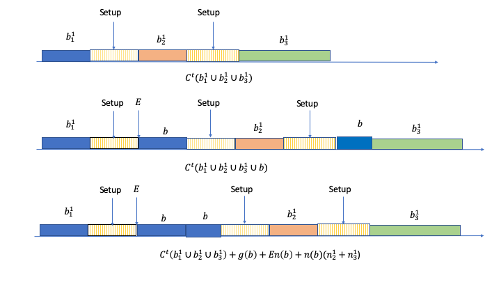
Figure A.2: Insert a Batch

Lemma 14.

Suppose $I$ is a job instance served by the online policy in a busy period, $b$ is a batch and $p_{min}=1$, then $C^{*}(I\cup b)\geq C^{*}(I)+g(b)+E^{*}n(b),$ where $E^{*}$ is the time when the server starts serving batch $b$ in the optimal solution.

Proof.

Since the earliest service time in the optimal solution for $b$ is at $E^{*}$, we have the minimal total completion time for $b$ is $g(b)+E^{*}n(b)$. ∎

We now introduce a benchmark for the online policy by combining the optimal solution and the truncated optimal solution. We let $C^{m}(I)=\alpha C^{*}(I)+(1-\alpha)C^{t}(I)$ be the benchmark, where $\alpha=\frac{1}{1+k}$ (in the proof we will see why $\alpha$ is given by this constant). We notice that $C^{*}(I)\geq C^{m}(I)\geq C^{t}(I)$ from the fact that $C^{*}(I)\geq C^{t}(I)$. If we have $\frac{C^{e}(I)}{C^{m}(I)}\leq\rho$, then we can show that $\frac{C^{e}(I)}{C^{*}(I)}\leq\rho$. The reason for introducing such a benchmark is that one can combine the results in Lemma 13 and Lemma 14 to provide a lower bound for $C^{m}(I\cup b)$ that contains both $E$ and $E^{*}$, as we will see later in the proof of Theorem 5.

Next we restate Theorem 5 in the main paper and describe the proof.

Theorem 15.

(Theorem 5 in the main paper) Any policy in $e\in\Pi_{r}$ has the competitive ratio $\kappa=\max\{\frac{k+1}{k}\gamma,k+1\}$ for the polling system $1\mid r_{i},\tau,p_{max}\leq\gamma p_{min}\mid\sum C_{i}$. When $\gamma\leq k$, for arbitrary $\epsilon>0$, there is an instance $I$ such that $\frac{C^{e}(I)}{C^{*}(I)}>\kappa-\epsilon=k+1-\epsilon$.

Proof.

We prove the theorem by induction. In this proof we only consider an instance $I$ that the online cyclic policy $e\in\Pi_{1}$ serves in a busy period. By induction we can finally conclude that $\frac{C^{e}(I)}{C^{m}(I)}\leq\kappa$ for instance $I$, which also implies that $\frac{C^{e}(I)}{C^{*}(I)}\leq\kappa.$ We first show that the batches served by the online policy in the first cycle, i.e., $I^{1}\in I$, satisfies $\frac{C^{e}(I^{1})}{C^{m}(I^{1})}\leq\kappa$. We next prove that if the result holds for $\cup_{j=1}^{w-1}I^{j}$, then it also holds for $(\cup_{j=1}^{w-1}I^{j})\cup b_{1}^{w}$. We then show the result for $(\cup_{j=1}^{w-1}I^{j})\cup(\cup_{i=1}^{l+1}b_{i}^{w})$ if the result holds for $(\cup_{j=1}^{w-1}I^{j})\cup(\cup_{i=1}^{l}b_{i}^{w})$.

We assume $p_{min}=1$ and $p_{max}=\gamma$ (the case where $p_{min}=0$ is similar). Notice that $I^{1}=\cup_{i=1}^{k}b_{i}^{1}$ is the union of batches served in the first cycle under the online policy. Without loss of generality, we assume the server serves from queue 1 to queue $k$ in each cycle. Knowing that $I^{1}=\cup_{i=1}^{k}b_{i}^{1}$, we let $n_{(k)}^{1}\geq n_{(k-1)}^{1}\geq...\geq n_{(1)}^{1}$ be the descending permutation of $(n_{1}^{1},...,n_{k}^{1})$, and $E^{1}=\min_{i=1}^{k}E_{i}^{1}$, $S^{1}=\min_{i=1}^{k}S_{i}^{1}$. Then we have (with explanation given later)

$$C^{t}(I^{1}) \geq g(I^{1})+\tau\sum_{i=2}^{k}\sum_{j=i}^{k}n_{(k-j+1)}^{1}+E^{1}\sum_{i=1}^{k}n_{i}^{1},$$ (A.1)

and

$$C^{e}(I^{1}) \leq \gamma g(I^{1})+\tau\sum_{i=2}^{k}\sum_{j=i}^{k}n_{(j)}^{1}+S^{1}\sum_{i=1}^{k}n_{i}^{1}.$$ (A.2)

The RHS of Inequality (A.1) is the minimal completion time of a list which has the same number of jobs in each queue as $I^{1}$ and all of these jobs arrive at time $E^{1}$ with each job having processing time 1. The first term $g(I^{1})$ is the pure completion time. The second term is because $n_{(k)}^{1}\geq n_{(k-1)}^{1}\geq...\geq n_{(1)}^{1}$, if all batches are available at time $E^{1}$ and there are no further arrivals, the best order of serving the batches is to serve from the longest one to the shortest one. Note that the optimal policy may start without setting up since it may be the same queue that the server was idling at and resumed with. In the case where there is no setup for the first queue, the completion time incurred by setup is $\tau\sum_{i=2}^{k}\sum_{j=i}^{k}n_{(k-j+1)}^{1}$. The third term in the RHS of Inequality (A.1) is because the entire service process for the truncated optimal solution starts from $E^{1}$. Therefore, the RHS of Inequality (A.1) is a lower bound for $C^{t}(I^{1})$. The RHS of inequality (A.2) is an upper bound for the online policy, which says that the online policy may serve batches from the shortest to the longest, starting from time point $S^{1}$, and all the processing times are bounded by $\gamma$. Since we consider I-B in this case, the server in the online policy does not set up for the first batch as the server was idling in the same queue as the new arrival. So the completion time resulted by setup is upper bounded by $\tau\sum_{i=2}^{k}\sum_{j=i}^{k}n_{(j)}^{1}$.

We let $Z(k)=\sum_{i=1}^{k}\sum_{j=i}^{k}n_{(j)}^{1}$ and $Z^{t}(k)=\sum_{i=1}^{k}\sum_{j=i}^{k}n_{(k-j+1)}^{1}$ then

$$\frac{Z(k)}{Z^{t}(k)} = \frac{kn_{(k)}^{1}+(k-1)n_{(k-1)}^{1}+...+n_{(1)}^{1}}{kn_{(1)}^{1}+(k-1)n_{(2)}^{1}+...+n_{(k)}^{1}}\leq\frac{kn_{(k)}^{1}+kn_{(k-1)}^{1}+...+kn_{(1)}^{1}}{n_{(1)}^{1}+n_{(2)}^{1}+...+n_{(k)}^{1}}\leq k.$$

From Fact 11 we have

$$\frac{C^{e}(I^{1})}{C^{t}(I^{1})} \leq \frac{\gamma g(I^{1})+\tau\sum_{i=2}^{k}\sum_{j=i}^{k}n_{(i)}^{1}+S^{1}\sum_{i=1}^{k}n_{i}^{1}}{g(I^{1})+\tau\sum_{i=2}^{k}\sum_{j=i}^{k}n_{(k-j+1)}^{1}+E^{1}\sum_{i=1}^{k}n_{i}^{1}}\leq\frac{\gamma g(I^{1})+\tau(Z(k)-\sum_{i=1}^{k}n_{i}^{1})+E^{1}\sum_{i=1}^{k}n_{i}^{1}}{g(I^{1})+\tau(Z^{t}(k)-\sum_{i=1}^{k}n_{i}^{1})+E^{1}\sum_{i=1}^{k}n_{i}^{1}}$$ (A.3)

$$\leq \max\{\gamma,k,1\}<\kappa.$$

The Inequality (A.3) follows from the fact that $\tau\leq\min_{i=1}^{k}S_{i}^{1}=\min_{i=1}^{k}\{R_{i}^{1}\}\leq\min_{i=1}^{k}E_{i}^{1}$ because there must be a busy period happening before an I-B.

So far we have shown $\frac{C^{e}(I^{1})}{C^{m}(I^{1})}\leq\kappa$ from the fact that $C^{t}(I^{1})\leq C^{m}(I^{1}).$ Now we prove that $C^{e}((\cup_{j=1}^{w-1}I^{j})\cup b_{1}^{w})\leq\kappa C^{m}((\cup_{j=1}^{w-1}I^{1})\cup b_{1}^{w})$. Clearly if $n_{1}^{w}=0$ then the conclusion holds. Now we let $\bar{n}=\sum_{j=1}^{w-1}\sum_{i=1}^{k}n_{i}^{j}+n_{1}^{w}$ and suppose $n_{1}^{w}\neq 0$, we then have

$$C^{e}((\cup_{j=1}^{w-1}I^{j})\cup b_{1}^{w}) \leq C^{e}(\cup_{j=1}^{w-1}I^{j})+\gamma g(b_{1}^{w})+n_{1}^{w}\left(\gamma\sum_{i=1}^{k}n_{i}^{w-1}+k\tau+S_{1}^{w-1}\right),$$ (A.4)

and

$$C^{m}((\cup_{j=1}^{w-1}I^{j})\cup b_{1}^{w}) = \alpha C^{*}((\cup_{j=1}^{w-1}I^{j})\cup b_{1}^{w})+(1-\alpha)C^{t}((\cup_{j=1}^{w-1}I^{j})\cup b_{1}^{w})$$ (A.5)

$$\geq \alpha C^{*}(\cup_{j=1}^{w-1}I^{j})+\alpha E_{1}^{w*}n_{1}^{w}+\alpha g(b_{1}^{w})$$

$$+(1-\alpha)C^{t}(\cup_{j=1}^{w-1}I^{j})+(1-\alpha)g(b_{1}^{w})$$

$$+(1-\alpha)E_{1}^{w}n_{1}^{w}+(1-\alpha)n_{1}^{w}(\bar{n}-q_{1}^{w}),$$

where

$$E_{1}^{w}\geq S^{1}+q_{1}^{w},$$ (A.6)

and

$$E_{1}^{w*}\geq R_{1}^{w}\geq S_{1}^{w-1}+n_{1}^{w-1}.$$ (A.7)

The RHS of Inequality (A.4) is because the completion time of batch $b_{1}^{w}$ is bounded by $\gamma$ times its pure completion time $g(b_{1}^{w}),$ which is the maximal pure completion time for $b_{1}^{w}$ (if processing time for each job in $b_{1}^{w}$ is $p_{max}=\gamma$), plus $n_{1}^{w}$ times the maximal starting time $\gamma\sum_{i=1}^{k}n_{i}^{w-1}+k\tau+S_{1}^{w-1}$. Inequality A.5 follows from Lemma 13 and 14 directly. Inequality (A.6) holds because before $E_{1}^{w}$, the server has served $q_{1}^{w}$ jobs. Inequality (A.7) is because the earliest time to serve $b_{1}^{w}$ is no earlier than $R_{1}^{w}$. From Inequalities (A.4,A.5,A.6 and A.7) we have

$$\frac{C^{e}((\cup_{j=1}^{w-1}I^{j})\cup b_{1}^{w})}{C^{m}((\cup_{j=1}^{w-1}I^{j})\cup b_{1}^{w})} \leq \frac{C^{e}(\cup_{j=1}^{w-1}I^{j})+\gamma g(b_{1}^{w})+n_{1}^{w}\left(\gamma\sum_{i=1}^{k}n_{i}^{w-1}+k\tau+S_{1}^{w-1}\right)}{\alpha C^{*}(\cup_{j=1}^{w-1}I^{j})+(1-\alpha)C^{t}(\cup_{j=1}^{w-1}I^{j})+\alpha S_{1}^{w-1}n_{1}^{w}+g(b_{1}^{w})+(1-\alpha)n_{1}^{w}\bar{n}+(1-\alpha)n_{1}^{w}\tau}$$

$$\leq \max\{\frac{C^{e}(\cup_{j=1}^{w-1}I^{j})}{C^{m}(\cup_{j=1}^{w-1}I^{j})},\frac{\gamma g(b_{1}^{w})}{g(b_{1}^{w})},\frac{k\tau+S_{1}^{w-1}}{\alpha S_{1}^{w-1}+(1-\alpha)\tau},\frac{\gamma\bar{n}}{(1-\alpha)\bar{n}}\}$$

$$\leq \max\{\kappa,\gamma,k+1,\frac{\gamma}{1-\alpha}\}.$$

Notice that $\max\{\kappa,\gamma,k+1,\frac{\gamma}{1-\alpha}\}=\max\{\kappa,\gamma,k+1,\gamma\frac{k+1}{k}\}=\kappa$ from the fact $\alpha=\frac{1}{k+1}.$

Now suppose the result holds for $\bar{b}=\left(\cup_{j=1}^{w-1}I^{j}\right)\cup\left(\cup_{i=1}^{l}b_{i}^{w}\right)$ where $w\geq 2$, and we want to show it also holds for $\bar{b}\cup b_{l+1}^{w}=\left(\cup_{j=1}^{w-1}I^{j}\right)\cup\left(\cup_{i=1}^{l+1}b_{i}^{w}\right)$ for $l<k$ by induction, where $n_{l+1}^{w}\neq 0$. We abuse the notion by letting $\bar{n}=\sum_{j=1}^{w-1}\sum_{i=1}^{k}n_{i}^{j}+\sum_{i=1}^{l}n_{i}^{w}$ be the number of jobs served before $b_{l+1}^{w}$, and $\bar{n}_{l+1}^{w}=\sum_{j=l+1}^{k}n_{j}^{w-1}+\sum_{j=1}^{l}n_{j}^{w}$ be the number of jobs served between $S_{l+1}^{w-1}$ and $S_{l+1}^{w}$. Because the server stays in queue $i$ at the $k^{th}$ visit for no more than time $\gamma n_{i}^{k}$ and serves $n_{i}^{k}$ jobs ,we have

$$C^{e}(\bar{b}\cup b_{l+1}^{w}) \leq C^{e}(\bar{b})+\gamma g(b_{l+1}^{w})+n_{l+1}^{w}\left(\gamma\bar{n}_{l+1}^{w}+k\tau+S_{l+1}^{w-1}\right),$$

and

$$C^{m}(\bar{b}\cup b_{l+1}^{w}) = \alpha C^{*}(\bar{b}\cup b_{l+1}^{w})+(1-\alpha)C^{t}(\bar{b}\cup b_{l+1}^{w})$$

$$\geq \alpha C^{*}(\bar{b})+\alpha E_{l+1}^{w*}n_{l+1}^{w}+\alpha g(b_{l+1}^{w})$$

$$+(1-\alpha)C^{t}(\bar{b})+(1-\alpha)g(b_{l+1}^{w})$$

$$+(1-\alpha)E_{l+1}^{w}n_{l+1}^{w}+(1-\alpha)n_{l+1}^{w}(\bar{n}-q_{l+1}^{w}),$$

where

$$E_{l+1}^{w} \geq \tau+q_{l+1}^{w},$$

and

$$E_{l+1}^{w*} \geq R_{l+1}^{w}>S_{l+1}^{w-1}+n_{l+1}^{w-1}$$ .

Similar to our discussion above, we have

$$\frac{C^{e}(\bar{b}\cup b_{l+1}^{w})}{C^{m}(\bar{b}\cup b_{l+1}^{w})} \leq \frac{C^{e}(\bar{b})+\gamma g(b_{l+1}^{w})+n_{l+1}^{w}\left(\gamma\bar{n}_{l+1}^{w}+k\tau+S_{l+1}^{w-1}\right)}{\alpha C^{*}(\bar{b})+(1-\alpha)C^{t}(\bar{b})+\alpha S_{l+1}^{w-1}n_{l+1}^{w}+g(b_{l+1}^{w})+(1-\alpha)n_{l+1}^{w}\bar{n}+(1-\alpha)n_{1}^{w}\tau}$$

$$\leq \max\{\frac{C^{e}(\bar{b})}{C^{m}(\bar{b})},\frac{\gamma g(b_{l+1}^{w})}{g(b_{l+1}^{w})},\frac{k\tau+S_{l+1}^{w-1}}{\alpha S_{l+1}^{w-1}+(1-\alpha)\tau},\frac{\gamma\bar{n}}{(1-\alpha)\bar{n}}\}$$

$$\leq \max\{\kappa,\gamma,k+1,\frac{\gamma}{1-\alpha}\}=\kappa.$$

Now we show that results hold for the second type of busy period, i.e., II-B. For II-B, the first arrival occurs in a different queue from where the server was idling, thus the server starts this period with a setup. Note that the very first busy period is also a II-B. If it is the first busy period, then we have

$$C^{t}(I^{1}) \geq g(I^{1})+\tau\sum_{i=1}^{k}\sum_{j=i}^{k}n_{(k-j+1)}^{1},$$

and

$$C^{e}(I^{1}) \leq \gamma g(I^{1})+\tau\sum_{i=1}^{k}\sum_{j=i}^{k}n_{(j)}^{1}+\tau\sum_{i=1}^{k}n_{i}^{1}.$$

Thus

$$\frac{C^{e}(I^{1})}{C^{t}(I^{1})} \leq \frac{\gamma g(I^{1})+\tau Z(k)+\tau\sum_{i=1}^{k}n_{i}^{1}}{g(I^{1})+\tau Z^{t}(k)}\leq\max\{\gamma,k+1\}\leq\kappa.$$

If it is not the very first busy period, then

$$C^{t}(I^{1}) \geq g(I^{1})+\tau\sum_{i=2}^{k}\sum_{j=i}^{k}n_{(k-j+1)}^{1}+E^{1}\sum_{i=1}^{k}n_{i}^{1},$$

and

$$C^{e}(I^{1}) \leq \gamma g(I^{1})+\tau\sum_{i=2}^{k}\sum_{j=i}^{k}n_{(j)}^{1}+S^{1}\sum_{i=1}^{k}n_{i}^{1}.$$

If $R^{1}<\tau$, then $S^{1}=R^{1}+\tau\leq 2\tau$, and $E^{1}\geq\tau.$ The argument is the same as the very first busy period, which we have discussed. Now we only need to discuss the case when $R^{1}\geq\tau,$ in which we have

$$\frac{C^{e}(I^{1})}{C^{t}(I^{1})} \leq \frac{\gamma g(I^{1})+\tau\sum_{i=2}^{k}\sum_{j=i}^{k}n_{(j)}^{1}+S^{1}\sum_{i=1}^{k}n_{i}^{1}}{g(I^{1})+\tau\sum_{i=2}^{k}\sum_{j=i}^{k}n_{(k-j+1)}^{1}+E^{1}\sum_{i=1}^{k}n_{i}^{1}}$$ (A.8)

$$\leq \frac{\gamma g(I^{1})+\tau\sum_{i=2}^{k}\sum_{j=i}^{k}n_{(j)}^{1}+(R^{1}+\tau)\sum_{i=1}^{k}n_{i}^{1}}{g(I^{1})+\tau\sum_{i=2}^{k}\sum_{j=i}^{k}n_{(k-j+1)}^{1}+R^{1}\sum_{i=1}^{k}n_{i}^{1}}$$

From the fact that $\frac{\gamma g(I^{1})+\tau\sum_{i=2}^{k}\sum_{j=i}^{k}n_{(j)}^{1}+(R^{1}+\tau)\sum_{i=1}^{k}n_{i}^{1}}{g(I^{1})+\tau\sum_{i=2}^{k}\sum_{j=i}^{k}n_{(k-j+1)}^{1}+R^{1}\sum_{i=1}^{k}n_{i}^{1}}$ is decreasing as $R^{1}$ increases, we have

$$\frac{\gamma g(I^{1})+\tau\sum_{i=2}^{k}\sum_{j=i}^{k}n_{(j)}^{1}+(R^{1}+\tau)\sum_{i=1}^{k}n_{i}^{1}}{g(I^{1})+\tau\sum_{i=2}^{k}\sum_{j=i}^{k}n_{(k-j+1)}^{1}+R^{1}\sum_{i=1}^{k}n_{i}^{1}} \leq \frac{\gamma g(I^{1})+\tau\sum_{i=2}^{k}\sum_{j=i}^{k}n_{(j)}^{1}+2\tau\sum_{i=1}^{k}n_{i}^{1}}{g(I^{1})+\tau\sum_{i=2}^{k}\sum_{j=i}^{k}n_{(k-j+1)}^{1}+\tau\sum_{i=1}^{k}n_{i}^{1}}$$

$$\leq \max\{\gamma,k+1\}\leq\kappa.$$

Discussion for $(\cup_{j=1}^{w-1}I^{j})\cup b_{l+1}^{w}$ for $l=0,...,k-1$ is similar to our discussion for I-B.

Now we prove the approximate tightness argument of this theorem by constructing a special instance $I$. When $\gamma\leq k$, we have $\kappa=k+1$. Suppose at time 0 there is one job with processing time $\gamma$ at queue 1 and one job with $p=1$ at the other queues. At time $\gamma+\tau+\epsilon_{1}$ (with small $\epsilon_{1}>0$) a batch $b_{1}^{2}$ arrives at queue 1 and each job in $b_{1}^{2}$ has processing time $p=1$. We thus have

$$C^{e}(I) \geq g(I)+n_{1}^{2}(k+1)\tau+\frac{k(k+1)}{2}\tau,$$

and

$$C^{*}(I) \leq \gamma g(I)+n_{1}^{2}(\tau+\epsilon_{1})+\frac{k(k+1)}{2}\tau+(k-1)\epsilon_{1}.$$

Thus when $\tau=(n_{1}^{2})^{2}$ there is an $n_{1}^{2}$ such that for arbitrary $\epsilon,$

$$\frac{C^{e}(I)}{C^{*}(I)} > 1+k-\epsilon.$$

The theorem also holds for $p_{max}=0$, for simplicity we do not show the proof here.

We now provide the proof for $\Pi_{2}$, however this time we only need to show $C^{ew}(I)\leq\kappa C^{m}(I)$ for any busy period $I$ where $C^{ew}(I)$ is the completion time by a policy from $\Pi_{2}$. Notice we no longer need to consider different cases for I-B and II-B because even when the system is idling, the cyclic policy still keeps setting up queues in cycle. When a new arrival occurs after the system being empty for some time, we simply regard this time $R^{1}$ as the beginning of a busy period. Without loss of generality, we assume the server begins serving with queue 1 in this busy period. Let $n_{(k)}^{1}\geq n_{(k-1)}^{1}\geq...\geq n_{(1)}^{1}$ be the descending permutation of $(n_{1}^{1},...,n_{k}^{1})$ , $R^{1}=\min_{i=1}^{k}R_{i}^{1}$ , $E^{1}=\min_{i=1}^{k}E_{i}^{1}$ and $S^{1}=\min_{i=1}^{k}S_{i}^{1}$. Notice some of $n_{(i)}^{1}$ may be zero (not all of them) but the server still sets up the queue even if the queue is empty. We have

$$C^{m}(I^{1}) \geq g(I^{1})+\tau\sum_{i=2}^{k}\sum_{j=i}^{k}n_{(k-j+1)}^{1}+E^{1}\sum_{i=1}^{k}n_{i}^{1},$$

and

$$C^{ew}(I^{1}) \leq \gamma g(I^{1})+\tau k\sum_{i=1}^{k}n_{(i)}^{1}+R^{1}\sum_{i=1}^{k}n_{i}^{1}.$$

To show $\frac{C^{ew}(I^{1})}{C^{m}(I^{1})}\leq\kappa$, by abusing the notation a little, we first let $Z(k)=k\sum_{i=1}^{k}n_{(i)}^{1}$ and $Z^{t}(k)=\sum_{i=1}^{k}\sum_{j=i}^{k}n_{(k-j+1)}^{1},$ so

$$\frac{Z(k)}{Z^{t}(k)}=\frac{kn_{(k)}^{1}+kn_{(k-1)}^{1}+...+kn_{(1)}^{1}}{kn_{(1)}^{1}+(k-1)n_{(2)}^{1}+...+n_{(k)}^{1}}\leq\frac{kn_{(k)}^{1}+kn_{(k-1)}^{1}+...+kn_{(1)}^{1}}{n_{(1)}^{1}+n_{(2)}^{1}+...+n_{(k)}^{1}}\leq k.$$

Thus

$$\frac{C^{ew}(I^{1})}{C^{m}(I^{1})} \leq \frac{\gamma g(I^{1})+\tau k\sum_{i=1}^{k}n_{(i)}^{1}+R^{1}\sum_{i=1}^{k}n_{i}^{1}}{g(I^{1})+\tau\sum_{i=2}^{k}\sum_{j=i}^{k}n_{(k-j+1)}^{1}+E^{1}\sum_{i=1}^{k}n_{i}^{1}}$$

$$= \frac{\gamma g(I^{1})+\tau k\sum_{i=1}^{k}n_{(i)}^{1}+R^{1}\sum_{i=1}^{k}n_{i}^{1}}{g(I^{1})+\tau\sum_{i=2}^{k}\sum_{j=i}^{k}n_{(k-j+1)}^{1}+\max\{\tau,R^{1}\}\sum_{i=1}^{k}n_{i}^{1}}$$

$$\leq \max\{\gamma,k+1\}$$

$$\leq \kappa.$$

Inequality (A) holds because if $R^{1}\leq\tau$, then

$$\frac{\gamma g(I^{1})+\tau k\sum_{i=1}^{k}n_{(i)}^{1}+R^{1}\sum_{i=1}^{k}n_{i}^{1}}{g(I^{1})+\tau\sum_{i=2}^{k}\sum_{j=i}^{k}n_{(k-j+1)}^{1}+E^{1}\sum_{i=1}^{k}n_{i}^{1}} \leq \frac{\gamma g(I^{1})+\tau k\sum_{i=1}^{k}n_{(i)}^{1}+\tau\sum_{i=1}^{k}n_{i}^{1}}{g(I^{1})+\tau\sum_{i=2}^{k}\sum_{j=i}^{k}n_{(k-j+1)}^{1}+\tau\sum_{i=1}^{k}n_{i}^{1}}$$

$$\leq \max\{\gamma,k+1\}.$$

And if $R^{1}>\tau,$ then

$$\frac{\gamma g(I^{1})+\tau k\sum_{i=1}^{k}n_{(i)}^{1}+R^{1}\sum_{i=1}^{k}n_{i}^{1}}{g(I^{1})+\tau\sum_{i=2}^{k}\sum_{j=i}^{k}n_{(k-j+1)}^{1}+E^{1}\sum_{i=1}^{k}n_{i}^{1}} \leq \frac{\gamma g(I^{1})+\tau(k+1)\sum_{i=1}^{k}n_{(i)}^{1}+(R^{1}-\tau)\sum_{i=1}^{k}n_{i}^{1}}{g(I^{1})+\tau\sum_{i=1}^{k}\sum_{j=i}^{k}n_{(k-j+1)}^{1}+(R^{1}-\tau)\sum_{i=1}^{k}n_{i}^{1}}$$

$$\leq \max\{\gamma,k+1,1\}.$$

The discussions for $(\cup_{j=1}^{w-1}I_{j})\cup b_{l+1}^{w}$ is similar to proof for $\Pi_{1}$.

We now show the proof for the policy set $\Pi_{4}$. The proof for $\Pi_{3}$ is similar to the proof for $\Pi_{1}$. We prove the theorem by induction. Again for simplicity, we assume $p_{min}=1$ so that $p_{max}=\gamma$. We want to show $C^{g}(I)\leq\kappa C^{m}(I)$ holds for any instance $I$, where $C^{g}(I)$ is the completion time for any policy $g\in\Pi_{4}$. Again we assume the server routes from queue 1 to queue $k$ in each cycle. Let $n_{(k)}^{1}\geq n_{(k-1)}^{1}\geq...\geq n_{(1)}^{1}$ is the descending permutation of $(n_{1}^{1},...,n_{k}^{1})$ and $E^{1}=\min_{i=1}^{k}E_{i}^{1}$ , $S^{1}=\min_{i=1}^{k}S_{i}^{1}$, we have

$$C^{t}(I^{1}) \geq g(I^{1})+\tau\sum_{i=2}^{k}\sum_{j=i}^{k}n_{(k-j+1)}^{1}+E^{1}\sum_{i=1}^{k}n_{i}^{1},$$

and

$$C^{g}(I^{1}) \leq \gamma g(I^{1})+\tau k\sum_{i=1}^{k}n_{(i)}^{1}+S^{1}\sum_{i=1}^{k}n_{i}^{1}.$$

The rest of discussions are similar to the proof for $\Pi_{1}$, except now we have $E_{l+1}^{w*}>R_{l+1}^{w}$ because the policy is gated.

Notation	Meaning	Notation	Meaning
$b_{i}^{w},$ $i=1,...,k$	The job instance that are served by the cyclic online policy during the $w^{th}$ visit ($w^{th}$ cycle) to queue $i$, within a busy period	$I^{w}$, $w=1,2,...$	$I^{w}=\cup_{i=1}^{k}b_{i}^{w}$, the union of instances that are served by the online policy during the $w^{th}$ cycle within a busy period
$n_{i}^{w}=n(b_{i}^{w}),$ $i=1,...,k$	The number of jobs in batch $b_{i}^{w}$	$\alpha=\frac{1}{k+1}$	A constant
$S_{i}^{w},$ $i=1,...,k$	The time when the online policy starts to serve batch $b_{i}^{w}$	$S^{1}=\min_{i=1}^{k}\{S_{i}^{1}\}$	The earliest staring time for $I^{1}$ by the online policy
$R_{i}^{w}$, $i=1,...,k$	The earliest release time (arrival time) of batch $b_{i}^{w}$	$R^{1}=\min_{i=1}^{k}\{R_{i}^{1}\}$	The earliest release time of $I^{1}$
$E_{i}^{w}$	The time when the truncated optimal offline policy starts to serve batch $b_{i}^{w}$	$E^{1}=\min_{i=1}^{k}\{E_{i}^{1}\}$	The earliest time when the truncated optimal offline policy starts to serve $I^{1}$
$E_{i}^{w*}$	The time when the optimal offline policy starts to serve batch $b_{i}^{w}$	$q_{i}^{w}$, $i=1,...,k$	The jobs in $(\cup_{j=1}^{w-1}I^{j})\cup(\cup_{l=1}^{i-1}b_{l}^{w})$ that have been served by the optimal policy before $E_{i}^{w}$
$g(I)=\frac{n(I)(n(I)+1)}{2}$	Pure completion time for instance $I$	Busy period	The time period when the system is non-empty
I-B	Type I busy period. The server (under the online policy) starts the new busy period without setting up	II-B	Type II busy period. The server (under the online policy) starts the new busy period by setting up

Table 4: List of Notations for Appendix

∎

References

• [1] Allahverdi, A. The third comprehensive survey on scheduling problems with setup times/costs. European Journal of Operational Research 246, 2 (2015), 345–378.
• [2] Allahverdi, A., Ng, C., Cheng, T.Β E., and Kovalyov, M.Β Y. A survey of scheduling problems with setup times or costs. European Journal of Operational Research 187, 3 (2008), 985–1032.
• [3] Allahverdi, A., and Soroush, H. The significance of reducing setup times/setup costs. European Journal of Operational Research 187, 3 (2008), 978–984.
• [4] Altman, E., Khamisy, A., and Yechiali, U. On elevator polling with globally gated regime. Queueing Systems 11, 1 (1992), 85–90.
• [5] Anderson, E.Β J., and Potts, C.Β N. Online scheduling of a single machine to minimize total weighted completion time. Mathematics of Operations Research 29, 3 (2004), 686–697.
• [6] Bansal, N., Kamphorst, B., and Zwart, B. Achievable performance of blind policies in heavy traffic. Mathematics of Operations Research 43, 3 (2018), 949–964.
• [7] Boon, M.Β A., Adan, I.Β J., Winands, E.Β M., and Down, D. Delays at signalized intersections with exhaustive traffic control. Probability in the Engineering and Informational Sciences 26, 3 (2012), 337–373.
• [8] Boon, M.Β A., VanΒ der Mei, R., and Winands, E.Β M. Applications of polling systems. Surveys in Operations Research and Management Science 16, 2 (2011), 67–82.
• [9] Boxma, O.Β J., Levy, H., and Weststrate, J.Β A. Efficient visit orders for polling systems. Performance Evaluation 18, 2 (1993), 103–123.
• [10] Chekuri, C., Motwani, R., Natarajan, B., and Stein, C. Approximation techniques for average completion time scheduling. SIAM Journal on Computing 31, 1 (2001), 146–166.
• [11] Chung, H., Un, C.Β K., and Jung, W.Β Y. Performance analysis of markovian polling systems with single buffers. Performance Evaluation 19, 4 (1994), 303–315.
• [12] Divakaran, S., and Saks, M. An online algorithm for a problem in scheduling with set-ups and release times. Algorithmica 60, 2 (2011), 301–315.
• [13] Epstein, L., and van Stee, R. Lower bounds for on-line single-machine scheduling. Theoretical Computer Science 299, 1 (2003), 439–450.
• [14] Ferguson, M.Β J., and Aminetzah, Y.Β J. Exact results for nonsymmetric token ring systems. IEEE Transactions on Communications 33, 3 (1985), 223–231.
• [15] Gautam, N. Analysis of queues: methods and applications. CRC Press, 2012.
• [16] Gittins, J., Glazebrook, K., and Weber, R. Multi-armed bandit allocation indices. John Wiley & Sons, 2011.
• [17] Goemans, M.Β X., Queyranne, M., Schulz, A.Β S., Skutella, M., and Wang, Y. Single machine scheduling with release dates. SIAM Journal on Discrete Mathematics 15, 2 (2002), 165–192.
• [18] Graham, R.Β L., Lawler, E.Β L., Lenstra, J.Β K., and Kan, A.Β R. Optimization and approximation in deterministic sequencing and scheduling: a survey. Annals of Discrete Mathematics 5 (1979), 287–326.
• [19] Hall, L.Β A., Schulz, A.Β S., Shmoys, D.Β B., and Wein, J. Scheduling to minimize average completion time: Off-line and on-line approximation algorithms. Mathematics of Operations Research 22, 3 (1997), 513–544.
• [20] Hinder, O., and Mason, A.Β J. A novel integer programing formulation for scheduling with family setup times on a single machine to minimize maximum lateness. European Journal of Operational Research 262, 2 (2017), 411–423.
• [21] Hoogeveen, J.Β A., and Vestjens, A.Β P. Optimal on-line algorithms for single-machine scheduling. In International Conference on Integer Programming and Combinatorial Optimization (1996), Springer, pp.Β 404–414.
• [22] Jan-pieter, L.Β D., Boxma, O.Β J., and vanΒ der Mei, R.Β D. On two-queue markovian polling systems with exhaustive service. Queueing Systems 78, 4 (2014), 287–311.
• [23] Kan, A.Β R. Machine scheduling problems: classification, complexity and computations. Springer Science & Business Media, 2012.
• [24] Konheim, A.Β G., Levy, H., and Srinivasan, M.Β M. Descendant set: an efficient approach for the analysis of polling systems. IEEE Transactions on Communications 42, 234 (1994), 1245–1253.
• [25] Lawler, E.Β L., Lenstra, J.Β K., Kan, A. H.Β R., and Shmoys, D.Β B. Sequencing and scheduling: Algorithms and complexity. Handbooks in Operations Research and Management Science 4 (1993), 445–522.
• [26] Lenstra, J.Β K., Shmoys, D.Β B., and Tardos, E. Approximation algorithms for scheduling unrelated parallel machines. Mathematical Programming 46, 1-3 (1990), 259–271.
• [27] Levy, H., and Sidi, M. Polling systems: applications, modeling, and optimization. IEEE Transactions on Communications 38, 10 (1990), 1750–1760.
• [28] Liu, Z., Nain, P., and Towsley, D. On optimal polling policies. Queueing Systems 11, 1-2 (1992), 59–83.
• [29] Lu, X., Sitters, R., and Stougie, L. A class of on-line scheduling algorithms to minimize total completion time. Operations Research Letters 31, 3 (2003), 232–236.
• [30] LΓΌbbecke, E., Maurer, O., Megow, N., and Wiese, A. A new approach to online scheduling: Approximating the optimal competitive ratio. ACM Transactions on Algorithms (TALG) 13, 1 (2016), 15.
• [31] Miculescu, D., and Karaman, S. Polling-systems-based autonomous vehicle coordination in traffic intersections with no traffic signals. IEEE Transactions on Automatic Control (2019).
• [32] Mosheiov, G., Oron, D., and Ritov, Y. Minimizing flow-time on a single machine with integer batch sizes. Operations Research Letters 33, 5 (2005), 497–501.
• [33] Ng, C., Cheng, T.Β E., Yuan, J., and Liu, Z. On the single machine serial batching scheduling problem to minimize total completion time with precedence constraints, release dates and identical processing times. Operations Research Letters 31, 4 (2003), 323–326.
• [34] Phillips, C., Stein, C., and Wein, J. Minimizing average completion time in the presence of release dates. Mathematical Programming 82, 1-2 (1998), 199–223.
• [35] Ruiz, R., and VΓ‘zquez-RodrΓ­guez, J.Β A. The hybrid flow shop scheduling problem. European Journal of Operational Research 205, 1 (2010), 1–18.
• [36] Sarkar, D., and Zangwill, W. Expected waiting time for nonsymmetric cyclic queueing systems – exact results and applications. Management Science 35, 12 (1989), 1463–1474.
• [37] Schulz, A.Β S., and Skutella, M. The power of $\alpha$-points in preemptive single machine scheduling. Journal of Scheduling 5, 2 (2002), 121–133.
• [38] Shen, L., DauzΓ¨re-PΓ©rΓ¨s, S., and Neufeld, J.Β S. Solving the flexible job shop scheduling problem with sequence-dependent setup times. European Journal of Operational Research 265, 2 (2018), 503–516.
• [39] Sitters, R. Competitive analysis of preemptive single-machine scheduling. Operations Research Letters 38, 6 (2010), 585–588.
• [40] Smith, D.Β R. A new proof of the optimality of the shortest remaining processing time discipline. Operations Research 26, 1 (1978), 197–199.
• [41] Stougie, L., and Vestjens, A.Β P. Randomized algorithms for on-line scheduling problems: how low can’t you go? Operations Research Letters 30, 2 (2002), 89–96.
• [42] Takagi, H. Queuing analysis of polling models. ACM Computing Surveys (CSUR) 20, 1 (1988), 5–28.
• [43] Tao, J., Chao, Z., and Xi, Y. A semi-online algorithm and its competitive analysis for a single machine scheduling problem with bounded processing times. Journal of Industrial and Management Optimization 6, 2 (2010), 269–282.
• [44] Tao, J., Chao, Z., Xi, Y., and Tao, Y. An optimal semi-online algorithm for a single machine scheduling problem with bounded processing time. Information Processing Letters 110, 8-9 (2010), 325–330.
• [45] Vallada, E., and Ruiz, R. A genetic algorithm for the unrelated parallel machine scheduling problem with sequence dependent setup times. European Journal of Operational Research 211, 3 (2011), 612–622.
• [46] vanΒ der Mei, R.Β D., and Roubos, A. Polling models with multi-phase gated service. Annals of Operations Research 198, 1 (2012), 25–56.
• [47] VanΒ Vuuren, M., and Winands, E.Β M. Iterative approximation of k-limited polling systems. Queueing Systems 55, 3 (2007), 161–178.
• [48] Vishnevskii, V., and Semenova, O. Mathematical methods to study the polling systems. Automation and Remote Control 67, 2 (2006), 173–220.
• [49] Wierman, A., Winands, E.Β M., and Boxma, O.Β J. Scheduling in polling systems. Performance Evaluation 64, 9 (2007), 1009–1028.
• [50] Wierman, A., and Zwart, B. Is tail-optimal scheduling possible? Operations Research 60, 5 (2012), 1249–1257.
• [51] Winands, E.Β M., Adan, I. J.-B.Β F., and van Houtum, G.-J. Mean value analysis for polling systems. Queueing Systems 54, 1 (2006), 35–44.
• [52] Zhang, L., and Wirth, A. Online machine scheduling with family setups. Asia-Pacific Journal of Operational Research 33, 04 (2016), 1650027.