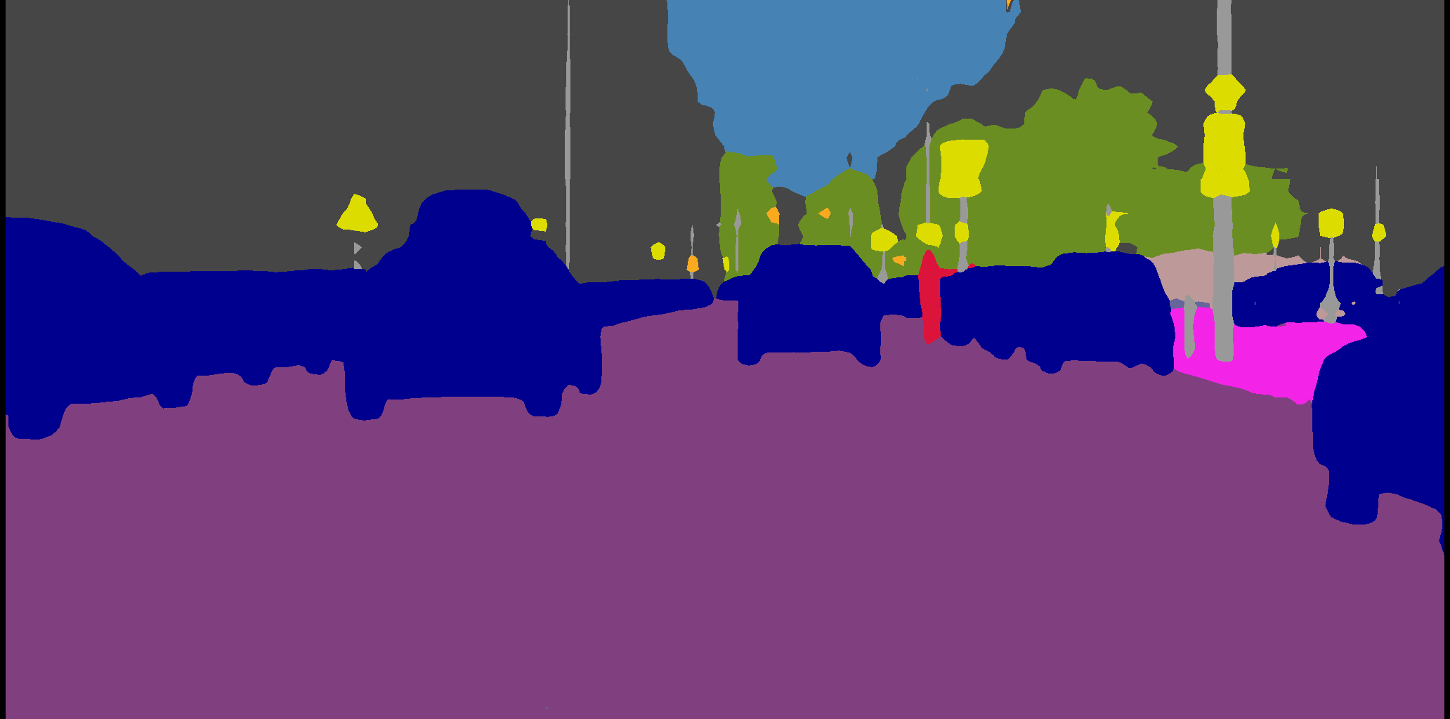
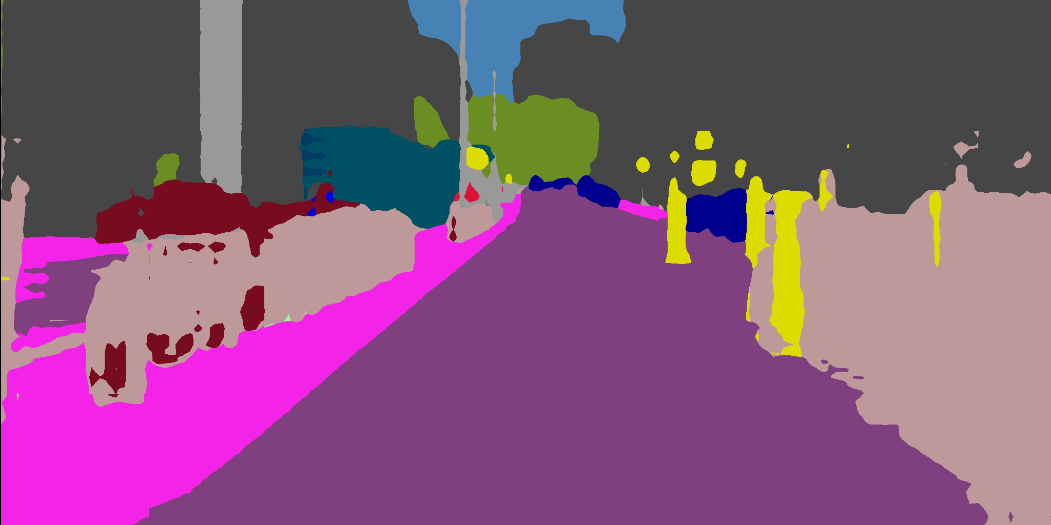
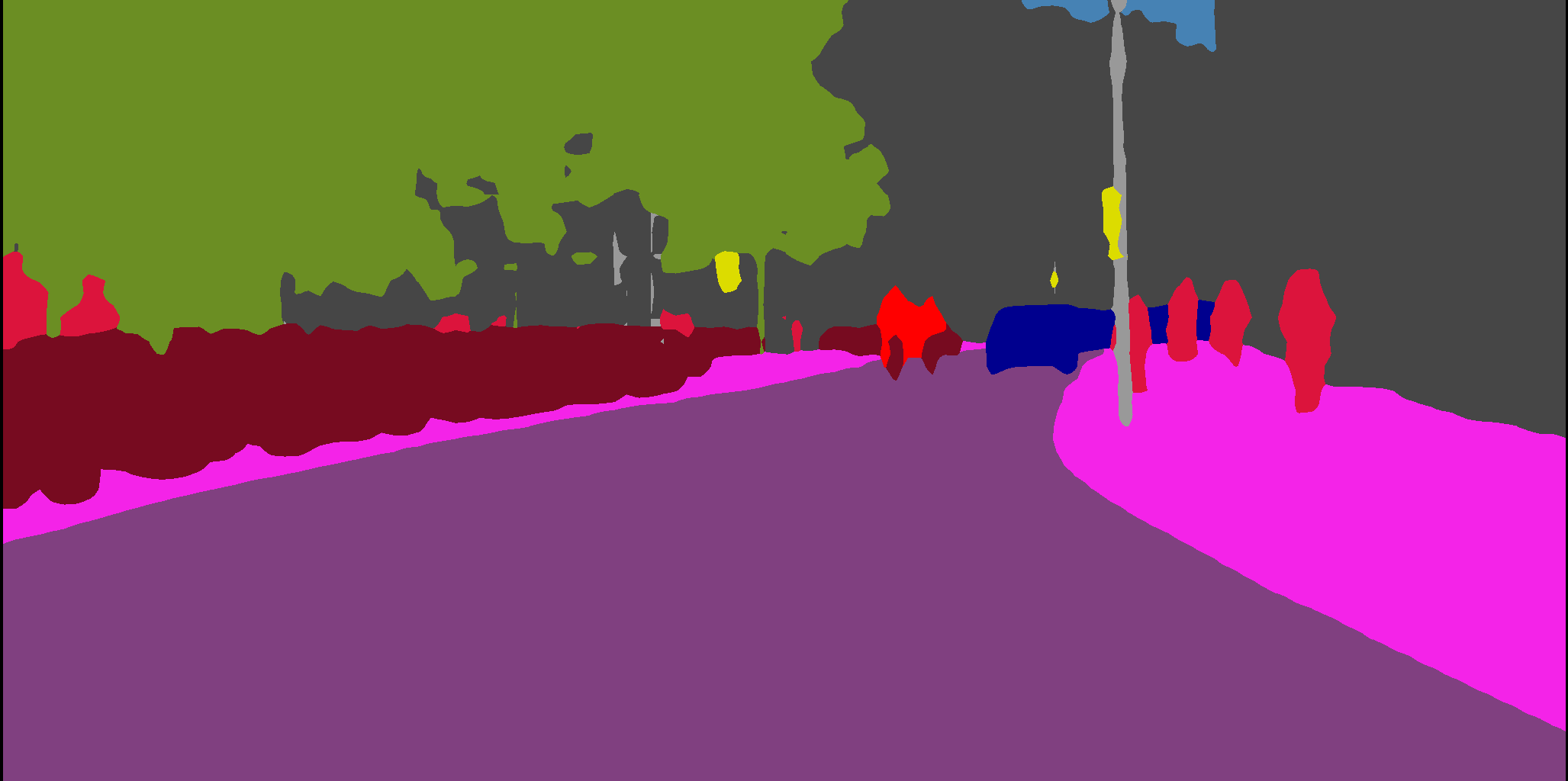
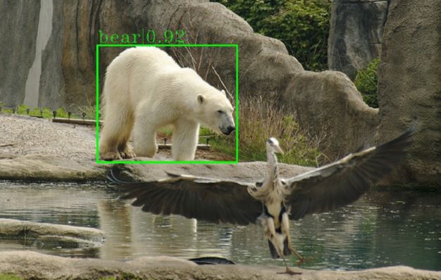
Fast Neural Network Adaptation via Parameter Remapping and Architecture Search
Abstract
Deep neural networks achieve remarkable performance in many computer vision tasks. Most state-of-the-art (SOTA) semantic segmentation and object detection approaches reuse neural network architectures designed for image classification as the backbone, commonly pre-trained on ImageNet. However, performance gains can be achieved by designing network architectures specifically for detection and segmentation, as shown by recent neural architecture search (NAS) research for detection and segmentation. One major challenge though, is that ImageNet pre-training of the search space representation (a.k.a. super network) or the searched networks incurs huge computational cost. In this paper, we propose a Fast Neural Network Adaptation (FNA) method, which can adapt both the architecture and parameters of a seed network (e.g. a high performing manually designed backbone) to become a network with different depth, width, or kernels via a Parameter Remapping technique, making it possible to utilize NAS for detection/segmentation tasks a lot more efficiently. In our experiments, we conduct FNA on MobileNetV2 to obtain new networks for both segmentation and detection that clearly out-perform existing networks designed both manually and by NAS. The total computation cost of FNA is significantly less than SOTA segmentation/detection NAS approaches: 1737 less than DPC, 6.8 less than Auto-DeepLab and 7.4 less than DetNAS. The code is available at https://github.com/JaminFong/FNA.
1 Introduction
Deep convolutional neural networks have achieved great successes in computer vision tasks such as image classification (Krizhevsky et al., 2012; He et al., 2016; Howard et al., 2017), semantic segmentation (Long et al., 2015; Ronneberger et al., 2015; Chen et al., 2017b) and object detection (Ren et al., 2015; Liu et al., 2016; Lin et al., 2017) etc. Image classification has always served as a fundamental task for neural architecture design. It is common to use networks designed and pre-trained on the classification task as the backbone and fine-tune them for segmentation or detection tasks. However, the backbone plays an important role in the performance on these tasks and the difference between these tasks calls for different design principles of the backbones. For example, segmentation tasks require high-resolution features and object detection tasks need to make both localization and classification predictions from each convolutional feature. Such distinctions make neural architectures designed for classification tasks fall short. Some attempts (Li et al., 2018; Wang et al., 2019) have been made to tackle this problem.
Handcrafted neural architecture design is inefficient, requires a lot of human expertise, and may not find the best-performing networks. Recently, neural architecture search (NAS) methods (Zoph et al., 2017; Pham et al., 2018; Liu et al., 2018) see a rise in popularity. Some works (Liu et al., 2019a; Zhang et al., 2019; Chen et al., 2019b) propose to use NAS to design backbone architectures specifically for segmentation or detection tasks. Nevertheless, pre-training remains a inevitable but costly procedure. Though some (He et al., 2018) recently demonstrates that pre-training is not always necessary for accuracy considerations, training from scratch on the target task still takes more iterations than fine-tuning from a pre-trained model. For NAS methods, the pre-training cost is non-negligible for evaluating the networks in the search space. One-shot search methods (Brock et al., 2017; Bender et al., 2018; Chen et al., 2019b) integrate all possible architectures in one super network but pre-training the super network and the searched network still bears huge computation cost.
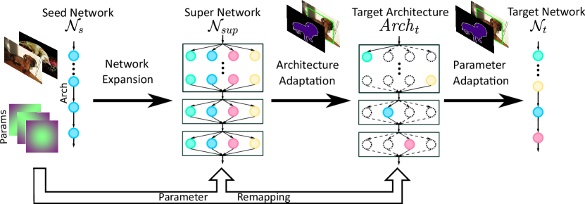
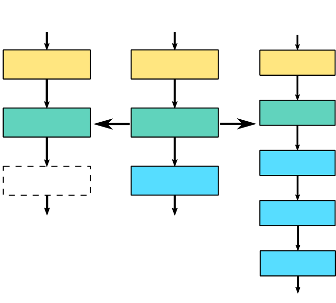
As ImageNet (Deng et al., 2009) pre-training has been a standard practice for many computer vision tasks, there are lots of models trained on ImageNet available in the community. To take full advantages of these models, we propose a Fast Neural Network Adaptation (FNA) method based on a novel parameter remapping paradigm. Our method can adapt both the architecture and parameters of one network to a new task with negligible cost. Fig. 1 shows the whole framework. The adaptation is performed on both the architecture- and parameter-level. We adopt the NAS methods (Zoph et al., 2017; Real et al., 2018; Liu et al., 2019b) to implement the architecture-level adaptation. We select a manually designed network (MobileNetV2 (Sandler et al., 2018) in our experiments) as the seed network, which is pre-trained on ImageNet. Then, we expand the seed network to a super network which is the representation of the search space in FNA. New parameters in the super network are initialized by mapping those from the seed network using parameter remapping. Thanks to that, the neural architecture search can be performed efficiently on the detection and segmentation tasks. With FNA we obtain a new optimal target architecture for the new task. Similarly, we remap the parameters of the seed network to the target architecture for initialization and fine-tune it on the target task with no need of pre-training on a large-scale dataset.
We demonstrate FNA’s effectiveness and efficiency via experiments on both segmentation and detection tasks. We adapt the manually designed network MobileNetV2 (Sandler et al., 2018) to segmentation framework DeepLabv3 (Chen et al., 2017b), detection framework RetinaNet (Lin et al., 2017) and SSDLite (Liu et al., 2016; Sandler et al., 2018). Networks adapted by FNA surpass both manually designed and NAS searched networks in terms of both performance and model MAdds. Compared to NAS methods, FNA costs 1737 less than DPC (Chen et al., 2018a), 6.8 less than Auto-DeepLab (Liu et al., 2019a) and 7.4 less than DetNAS (Chen et al., 2019b).
2 Related Work
Neural Architecture Search
With reinforcement learning (RL) and evolutionary algorithm (EA) being applied to NAS methods, many works (Zoph & Le, 2016; Zoph et al., 2017; Real et al., 2018) make great progress in promoting the performances of neural networks. Recently, NAS methods based on one-shot model (Brock et al., 2017; Bender et al., 2018) or differentiable representations (Liu et al., 2019b; Cai et al., 2019; Fang et al., 2019b) achieve remarkable results with low search cost. We use the differentiable NAS method to implement architecture adaptation, which adjusts the architecture of the backbone network automatically.
Backbone Design
As deep neural network designing (Simonyan & Zisserman, 2014; Szegedy et al., 2016; He et al., 2016) develops, the backbones of segmentation or detection networks evolve accordingly. Some works improve the backbone architectures by modifying existing networks. PeleeNet (Wang et al., 2018) proposes a variant of DenseNet (Huang et al., 2017) for more real-time object detection on mobile devices. DetNet (Li et al., 2018) applies dilated convolution (Yu & Koltun, 2016) in the backbone to enlarge the receptive field which helps to detect objects. BiSeNet (Yu et al., 2018) and HRNet (Wang et al., 2019) design multiple paths to learn both high- and low- resolution representations for better dense prediction.
Parameter Remapping
Net2Net (Chen et al., 2015) proposes the function-preserving transformations to remap the parameters of one network to a new deeper or wider network. This remapping mechanism accelerates the training of the new larger network and achieves great performances. Following this manner, EAS (Cai et al., 2018) extends the parameter remapping concept to neural architecture search. Moreover, some NAS works (Pham et al., 2018; Fang et al., 2019a; Elsken et al., 2019) apply parameters sharing on child models to accelerate the search process. Our parameter remapping paradigm extends the mapping dimension with the kernel level. Parameters can be also mapped to a shallower or narrower network with our scheme, while Net2Net focuses on mapping parameters to a deeper and wider network. The parameter remapping in our FNA largely decreases the computation cost of the network adaptation by taking full advantages of the ImageNet pre-trained parameters.
3 Method
As the most commonly used network for designing search spaces in NAS methods (Tan et al., 2018; Cai et al., 2019; Fang et al., 2019b), MobileNetV2 (Sandler et al., 2018) is selected as the seed network to give the details of our method. To adapt the network to segmentation and detection tasks, we adjust the architecture elements on three levels, i.e., convolution kernel size, depth and width of the network. In this section, we first describe the parameter remapping paradigm. Then we explain the whole procedure of the network adaptation.
3.1 Parameter Remapping
We define parameter remapping as one paradigm which aims at mapping the parameters of one seed network to another one. We denote the seed network as and the new network as , whose parameters are denoted as and respectively. The remapping paradigm is illustrated in the following three aspects. The remapping on the depth-level is firstly carried out and then the remapping on the kernel- and width- level is conducted simultaneously. Moreover, we study different remapping strategies in the experiments (Sec. 4.5).
Remapping on Depth-level
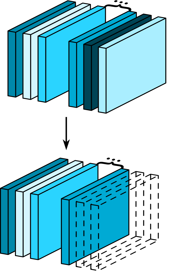
We introduce more depth settings in our architecture adaptation process. In other word, we adjust the number of inverted residual blocks (MBConvs) (Sandler et al., 2018) in every stage of the network. We assume that one stage in the seed network has layers. The parameters of each layer can be denoted as . Similarly, we assume that the corresponding stage with layers in the new network has parameters . The remapping process on the depth-level is shown in Fig. 2(a). The parameters of layers in which also exit in are just copied from . The parameters of new layers are all copied from the last layer in the stage of . It is formulated as
| (1) | ||||
Remapping on Width-level
In the MBConv block of MobileNetV2 (Sandler et al., 2018) network, the first point-wise convolution expands the low-dimensional features to a high dimension. This practice can be utilized for expanding the width and capacity of one neural network. We allow smaller expansion ratios for architecture adaptation. We denote the parameters of one convolution in as and that in as , where and . As shown in Fig. 2(b), on the width-level, we directly map the first or channels of parameters in to the narrower one in . It can be formulated as
| (2) |
Remapping on Kernel-level
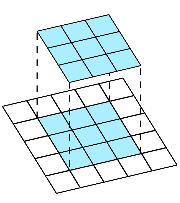
The kernel size is commonly set as in most artificially-designed networks. To expand the receptive field and capture abundant features in segmentation or detection tasks, we introduce larger kernel size settings in the adaptation process. As Fig. 2(c) shows, to expand the kernel to a larger one, we assign the parameters of the central region in the large kernel with the values of the original kernel. The values of the other region surrounding the central part are assigned with 0. We denote the parameters of the original kernel as and the larger kernel as . The remapping process on kernel-level can be formulated as follows,
| (3) |
where denote the indices of the spatial dimension. This design principle conforms to the function-preserving concept (Chen et al., 2015), which accelerates and stabilizes the optimization of the new network.
3.2 Neural Network Adaptation
We divide our neural network adaptation into three steps. Fig. 1 demonstrates the whole adaptation procedure. Firstly, we expand the seed network to a super network which is the representation of the search space in the latter architecture adaptation process. Secondly, we perform the differentiable NAS method to implement network adaptation on the architecture-level and obtain the target architecture . Finally, we adapt the parameters of the target architecture and obtain the target network . The aforementioned parameter remapping mechanism is deployed before the two stages, i.e. architecture adaptation and parameter adaptation.
Network Expansion
We expand the seed network to a super network by introducing more options for architecture elements. For every MBConv layer, we allow for more kernel size settings and more expansion ratios . As most differentiable NAS methods (Liu et al., 2019b; Cai et al., 2019; Wu et al., 2018) do, we relax every layer as a weighted sum of all candidate operations.
| (4) |
where denotes the operation set, denotes the architecture parameter of operation in the th layer, and denotes the input tensor. We set more layers in one stage of the super network and add the identity connection to the candidate operation set for depth search. After expanding the seed network to a super network, we remap the parameters of the seed network to the super network based on the paradigm illustrated in Sec. 3.1. This remapping strategy prevents the huge cost of ImageNet pre-training involved in the search space, i.e. the super network in differentiable NAS.
Architecture Adaptation
We start the differentiable NAS process with the expanded super network directly on the target task, e.g., semantic segmentation or object detection. We first fine-tune operation weights of the super network for some epochs on the training dataset. After the weights are sufficiently trained, we start alternating the optimization of operation weights with and architecture parameters with . To accelerate the search process and decouple the parameters of different sub-networks, we only sample one path in each iteration according to the distribution of architecture parameters for operation weight updating. As the search process terminates, we use the architecture parameters to derive the target architecture.
Parameter Adaptation
We obtain the target architecture from architecture adaptation. To accommodate the new segmentation or detection tasks, the target architecture becomes different from that of the seed network (which is primitively designed for the image classification task). Unlike conventional training strategy, we discard the cumbersome pre-training process of on ImageNet. We remap the parameters of to utilizing the method described in Sec. 3.1. Finally, we directly fine-tune on the target task and obtain the final target network .
4 Experiments
We select the ImageNet pre-trained MobileNetV2 model as the seed network and apply our FNA method on both semantic segmentation and object detection tasks. In this section, we firstly give the implementation details of our experiments; then we report and analyze the network adaptation results; finally, we perform ablation studies to validate the effectiveness of the parameter remapping paradigm and compare different parameter remapping implementations.
| Method | OS | iters | Params | MAdds | mIOU(%) | |
|---|---|---|---|---|---|---|
| MobileNetV2 (Sandler et al., 2018) | DeepLabv3 | 16 | 100K | 2.57M | 24.52B | 75.5 |
| DPC (Chen et al., 2018a) | 2.51M | 24.69B | 75.4(75.7) | |||
| FNA | 2.47M | 24.17B | 76.6 | |||
| Auto-DeepLab-S (Liu et al., 2019a) | DeepLabv3+ | 8 | 500K | 10.15M | 333.25B | 75.2 |
| FNA | 16 | 100K | 5.71M | 210.11B | 77.2 | |
| FNA | 8 | 100K | 5.71M | 313.87B | 78.0 | |
4.1 Network Adaptation on Semantic Segmentation
The semantic segmentation experiments are conducted on the Cityscapes (Cordts et al., 2016) dataset. In the architecture adaptation process, we map the seed network to the super network, which is used as the backbone of DeepLabv3 (Chen et al., 2017b). We randomly sample images from the training set as the validation set for architecture parameters updating. The original validation set is not used in the search process. To optimize the MAdds of the searched network, we define the loss function in search as . The first term denotes the cross-entropy loss and the second term controls the MAdds of the network. We set as and as . The search process takes epochs in total. The architecture optimization starts after epochs. The whole search process is conducted on a single V100 GPU and takes only 1.4 hours in total.
In the parameter adaptation process, we remap the parameters of original MobileNetV2 to the target architecture obtained in the aforementioned architecture adaptation. The whole parameter adaptation process is conducted on TITAN-Xp GPUs and takes K iterations, which cost only hours in total.
Our semantic segmentation results are shown in Tab. 1. The FNA network achieves mIOU on Cityscapes with the DeepLabv3 (Chen et al., 2017b) framework, mIOU better than the manually designed seed Network MobileNetV2 (Sandler et al., 2018) with fewer MAdds. Compared with a NAS method DPC (Chen et al., 2018a) (with MobileNetV2 as the backbone) which searches a multi-scale module for semantic segmentation tasks, FNA gets mIOU promotion with B fewer MAdds. For fair comparison with Auto-DeepLab (Liu et al., 2019a) which searches the backbone architecture on DeepLabv3 and retrains the searched network on DeepLabv3+ (Chen et al., 2018b), we adapt the parameters of the target architecture to DeepLabv3+ framework. Comparing with Auto-DeepLab-S, FNA achieves far better mIOU with fewer MAdds, Params and training iterations. With the remapping mechanism, FNA only takes 35.8 GPU hours, 1737 less than DPC and 6.8 less than Auto-DeepLab.
| Method | Params | MAdds | mAP(%) | |
|---|---|---|---|---|
| ShuffleNetV2-20 (Chen et al., 2019b) | RetinaNet | 13.19M | 132.76B | 32.1 |
| MobileNetV2 (Sandler et al., 2018) | 11.49M | 133.05B | 32.8 | |
| DetNAS (Chen et al., 2019b) | 13.41M | 133.26B | 33.3 | |
| FNA | 11.73M | 133.03B | 33.9 | |
| MobileNetV2 (Sandler et al., 2018) | SSDLite | 4.3M | 0.8B | 22.1 |
| Mnasnet-92 (Tan et al., 2018) | 5.3M | 1.0B | 22.9 | |
| FNA | 4.6M | 0.9B | 23.3 | |
| Method | Total Cost | Super Network | Target Network | |||
|---|---|---|---|---|---|---|
| Pre-training | Finetuning | Search | Pre-training | Finetuning | ||
| DetNAS (Chen et al., 2019b) | 68 GDs | 12 GDs | 12 GDs | 20 GDs | 12 GDs | 12 GDs |
| FNA (RetinaNet) | 9.2 GDs | - | - | 6 GDs | - | 3.2 GDs |
| FNA (SSDLite) | 21.6 GDs | - | - | 6.6 GDs | - | 15 GDs |
4.2 Network Adaptation on Object Detection
We further implement our FNA method on object detection tasks. We adapt the MobileNetV2 seed network to two commonly used detection systems, RetinaNet (Lin et al., 2017) and a lightweight one SSDLite (Liu et al., 2016; Sandler et al., 2018). The experiments are conducted on the MS-COCO dataset (Lin et al., 2014b). Our implementation is based on the MMDetection (Chen et al., 2019a) framework. In the search process of architecture adaptation, we randomly sample data from the original trainval35k set as the validation set.
We show the results on the COCO dataset in Tab. 3. In the RetinaNet framework, compared with two manually designed networks, ShuffleNetV2-10 (Ma et al., 2018; Chen et al., 2019b) and MobileNetV2 (Sandler et al., 2018), FNA achieves higher mAP with similar MAdds. Compared with DetNAS (Chen et al., 2019b) which searches the backbone of detection network, FNA achieves higher mAP with M fewer Params and B fewer MAdds. As shown in Tab. 4, our total computation cost is only 13.5% of DetNAS. Moreover, we implement our FNA method on the SSDLite framework. In Tab. 3, FNA surpasses both the manually designed network MobileNetV2 and the NAS-searched network MnasNet-92, where MnasNet (Tan et al., 2018) takes around 3.8K GPU days to search for the backbone network on ImageNet. The specific cost FNA takes on SSDLite is shown in Tab. 4. It is difficult to train the small network due to the simplification (Liu et al., 2019c). Therefore, experiments on SSDLite need long training schedule and take larger computation cost. The experimental results further demonstrate the efficiency and effectiveness of direct adaptation on the target task with parameter remapping.
4.3 Effectiveness of Parameter Remapping
To evaluate the effectiveness of the parameter remapping paradigm in our method, we attempt to optionally remove the parameter remapping process before the two stages, i.e. architecture adaptation and parameter adaptation. The experiments are conducted with the DeepLabv3 (Chen et al., 2017b) semantic segmentation framework on the Cityscapes dataset (Cordts et al., 2016).
| Row Num | Method | MAdds(B) | mIOU(%) |
|---|---|---|---|
| (1) | Remap ArchAdapt Remap ParamAdapt (FNA) | 24.17 | 76.6 |
| (2) | RandInit ArchAdapt Remap ParamAdapt | 24.29 | 76.0 |
| (3) | Remap ArchAdapt RandInit ParamAdapt | 24.17 | 73.0 |
| (4) | RandInit ArchAdapt RandInit ParamAdapt | 24.29 | 72.4 |
| (5) | Remap ArchAdapt Retrain ParamAdapt | 24.17 | 76.5 |
In Row (2) we remove the parameter remapping process before architecture adaptation. In other word, the search is performed from scratch without using the pre-trained network. The mIOU in Row (2) drops by 0.6% compared to FNA in Row (1). Then we remove the parameter remapping before parameter adaptation in Row (3), i.e. training the target architecture from scratch on the target task. The mIOU decreases by 3.6% compared the result of FNA. When we remove the parameter remapping before both stages in Row (4), it gets the worst performance. In Row (5), we first pre-train the searched architecture on ImageNet and then fine-tune it on the target task. It is worth noting that FNA even achieves a higher mIOU by a narrow margin (0.1%) than the ImageNet pre-trained one in Row (5). We conjecture that this may benefit from the regularization effect of parameter remapping before the parameter adaptation stage.
All the experiments are conducted using the same searching and training settings for fair comparisons. With parameter remapping applied on both stages, the adaptation achieves the best results in Tab. 5. Especially, the remapping process before parameter adaptation tends to provide greater performance gains than the remapping before architecture adaptation. All the experimental results demonstrate the importance and effectiveness of the proposed parameter remapping scheme.
| Row Num | Method | MAdds(B) | mAP(%) |
|---|---|---|---|
| (1) | DetNAS (Chen et al., 2019b) | 133.26 | 33.3 |
| (2) | Remap DiffSearch Remap ParamAdapt (FNA) | 133.03 | 33.9 |
| (3) | Remap RandSearch Remap ParamAdapt | 133.11 | 33.5 |
| (4) | RandInit RandSearch Remap ParamAdapt | 133.08 | 31.5 |
| (5) | Remap RandSearch RandInit ParamAdapt | 133.11 | 25.3 |
| (6) | RandInit RandSearch RandInit ParamAdapt | 133.08 | 24.9 |
4.4 Random Search Experiments
We carry out the Random Search (RandSearch) experiments with the RetinaNet (Lin et al., 2017) framework on the MS-COCO (Lin et al., 2014a) dataset. All the results are shown in the Tab. 6. We purely replace the original differentiable NAS (DiffSearch) method in FNA with the random search method in Row (3). The random search takes the same computation cost as the search in FNA for fair comparisons. We observe that FNA with RandSearch achieves comparable results with our original method. It further confirms that FNA is a general framework for network adaptation and has great generalization. NAS is only an implementation tool for architecture adaptation. The whole framework of FNA can be treated as a NAS-method agnostic mechanism. It is worth noting that even using random search, our FNA still outperforms DetNAS (Chen et al., 2019b) with 0.2% mAP better and 150M MAdds fewer.
We further conduct similar ablation studies with experiments in Sec. 4.3 about the parameter remapping scheme in Row (4) - (6). All the experiments further support the effectiveness of the parameter remapping scheme.
4.5 Study on Parameter Remapping
We explore more strategies for the Parameter Remapping paradigm. Similar to Sec. 4.3, all the experiments are conducted with the DeepLabv3 (Chen et al., 2017b) framework on the Cityscapes dataset (Cordts et al., 2016). We make exploration from the following respects. For simplicity, we denote the weights of the seed network and the new network on the remapping dimension (output/input channel) as and , where .
Remapping with BN Statistics on Width-level
We review the formulation of batch normalization (Ioffe & Szegedy, 2015) as follows,
| (5) |
where denotes the -dimensional input tensor of the th layer, denotes the learnable parameter which scales the normalized data on the channel dimension. We compute the absolute values of as . When remapping the parameters on the width-level, we sort the values of and map the parameters with the sorted top- indices. More specifically, we define a weights remapping function in Algo. 1, where the reference vector is .
Remapping with Weight Importance on Width-level
We attempt to utilize a canonical form of convolution weights to measure the importance of parameters. Then we remap the seed network parameters with great importance to the new network. The remapping operation is conducted based on Algo. 1 as well. We experiment with two canonical forms of weights to compute the reference vector, the standard deviation of as and the norm of as .
| Method | Width-BN | Width-Std | Width-L1 | Kernel-Dilate | FNA |
|---|---|---|---|---|---|
| mIOU(%) | 75.8 | 75.8 | 75.3 | 75.6 | 76.6 |
Remapping with Dilation on Kernel-level
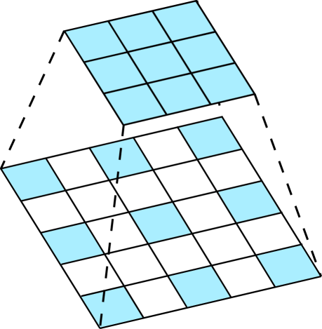
We experiment with another strategy of parameter remapping on the kernel-level. Different from the function-preserving method defined in Sec. 3.1, we remap the parameters with a dilation manner as shown in Fig. 3. The values in the convolution kernel without remapping are all assigned as . It is formulated as
| (6) |
where and denote the weights of the new network and the seed network respectively, denote the spatial indices.
Tab. 7 shows the experimental results. The network adaptation with the parameter remapping paradigm define in FNA achieves the best results. Furthermore, the remapping operation of FNA is easier to implement compared to the several aforementioned ones. However, we explore limited number of methods to implement the parameter remapping paradigm. How to conduct the remapping strategy more efficiently remains a significative future work.
5 Conclusion
In this paper, we propose a fast neural network adaptation method (FNA) with a parameter remapping paradigm and the architecture search method. We adapt the manually designed network MobileNetV2 to semantic segmentation and detection tasks on both architecture- and parameter- level. The parameter remapping strategy takes full advantages of the seed network parameters, which greatly accelerates both the architecture search and parameter fine-tuning process. With our FNA method, researchers and engineers could fast adapt more manually designed networks to various frameworks on different tasks. As there are lots of ImageNet pre-trained models available in the community, we could conduct adaptation with low cost and do more applications, e.g., face recognition, pose estimation, depth estimation, etc. We leave more efficient remapping strategies and more applications for future work.
Acknowledgement
This work was supported by National Natural Science Foundation of China (NSFC) (No. 61876212, No. 61733007 and No. 61572207), National Key R&D Program of China (No. 2018YFB1402600) and HUST-Horizon Computer Vision Research Center. We thank Liangchen Song, Yingqing Rao and Jiapei Feng for the discussion and assistance.
References
- Bender et al. (2018) Gabriel Bender, Pieter-Jan Kindermans, Barret Zoph, Vijay Vasudevan, and Quoc V. Le. Understanding and simplifying one-shot architecture search. In ICML, 2018.
- Brock et al. (2017) Andrew Brock, Theodore Lim, James M. Ritchie, and Nick Weston. SMASH: one-shot model architecture search through hypernetworks. arXiv:1708.05344, 2017.
- Cai et al. (2018) Han Cai, Tianyao Chen, Weinan Zhang, Yong Yu, and Jun Wang. Efficient architecture search by network transformation. In AAAI, 2018.
- Cai et al. (2019) Han Cai, Ligeng Zhu, and Song Han. ProxylessNAS: Direct neural architecture search on target task and hardware. In ICLR, 2019.
- Chen et al. (2019a) Kai Chen, Jiaqi Wang, Jiangmiao Pang, Yuhang Cao, Yu Xiong, Xiaoxiao Li, Shuyang Sun, Wansen Feng, Ziwei Liu, Jiarui Xu, Zheng Zhang, Dazhi Cheng, Chenchen Zhu, Tianheng Cheng, Qijie Zhao, Buyu Li, Xin Lu, Rui Zhu, Yue Wu, and Dahua Lin. Mmdetection: Open mmlab detection toolbox and benchmark. arXiv:1906.07155, 2019a.
- Chen et al. (2017a) Liang-Chieh Chen, George Papandreou, Iasonas Kokkinos, Kevin Murphy, and Alan L Yuille. Deeplab: Semantic image segmentation with deep convolutional nets, atrous convolution, and fully connected crfs. TPAMI, 2017a.
- Chen et al. (2017b) Liang-Chieh Chen, George Papandreou, Florian Schroff, and Hartwig Adam. Rethinking atrous convolution for semantic image segmentation. arXiv:1706.05587, 2017b.
- Chen et al. (2018a) Liang-Chieh Chen, Maxwell D. Collins, Yukun Zhu, George Papandreou, Barret Zoph, Florian Schroff, Hartwig Adam, and Jonathon Shlens. Searching for efficient multi-scale architectures for dense image prediction. In NeurIPS, 2018a.
- Chen et al. (2018b) Liang-Chieh Chen, Yukun Zhu, George Papandreou, Florian Schroff, and Hartwig Adam. Encoder-decoder with atrous separable convolution for semantic image segmentation. In ECCV, 2018b.
- Chen et al. (2015) Tianqi Chen, Ian J. Goodfellow, and Jonathon Shlens. Net2net: Accelerating learning via knowledge transfer. arXiv:1511.05641, 2015.
- Chen et al. (2019b) Yukang Chen, Tong Yang, Xiangyu Zhang, Gaofeng Meng, Chunhong Pan, and Jian Sun. Detnas: Neural architecture search on object detection. In NeurIPS, 2019b.
- Cordts et al. (2016) Marius Cordts, Mohamed Omran, Sebastian Ramos, Timo Rehfeld, Markus Enzweiler, Rodrigo Benenson, Uwe Franke, Stefan Roth, and Bernt Schiele. The cityscapes dataset for semantic urban scene understanding. In CVPR, 2016.
- Deng et al. (2009) Jia Deng, Wei Dong, Richard Socher, Li-Jia Li, Kai Li, and Fei-Fei Li. Imagenet: A large-scale hierarchical image database. In CVPR, 2009.
- Elsken et al. (2019) Thomas Elsken, Jan Hendrik Metzen, and Frank Hutter. Efficient multi-objective neural architecture search via lamarckian evolution. In ICLR, 2019.
- Fang et al. (2019a) Jiemin Fang, Yukang Chen, Xinbang Zhang, Qian Zhang, Chang Huang, Gaofeng Meng, Wenyu Liu, and Xinggang Wang. EAT-NAS: elastic architecture transfer for accelerating large-scale neural architecture search. arXiv:1901.05884, 2019a.
- Fang et al. (2019b) Jiemin Fang, Yuzhu Sun, Qian Zhang, Yuan Li, Wenyu Liu, and Xinggang Wang. Densely connected search space for more flexible neural architecture search. arXiv:1906.09607, 2019b.
- He et al. (2016) Kaiming He, Xiangyu Zhang, Shaoqing Ren, and Jian Sun. Deep residual learning for image recognition. In CVPR, 2016.
- He et al. (2018) Kaiming He, Ross B. Girshick, and Piotr Dollár. Rethinking imagenet pre-training. arXiv:1811.08883, 2018.
- Howard et al. (2017) Andrew G. Howard, Menglong Zhu, Bo Chen, Dmitry Kalenichenko, Weijun Wang, Tobias Weyand, Marco Andreetto, and Hartwig Adam. Mobilenets: Efficient convolutional neural networks for mobile vision applications. arXiv:1704.04861, 2017.
- Huang et al. (2017) Gao Huang, Zhuang Liu, Laurens van der Maaten, and Kilian Q. Weinberger. Densely connected convolutional networks. In CVPR, 2017.
- Ioffe & Szegedy (2015) Sergey Ioffe and Christian Szegedy. Batch normalization: Accelerating deep network training by reducing internal covariate shift. In ICML, 2015.
- Kingma & Ba (2015) Diederik P. Kingma and Jimmy Ba. Adam: A method for stochastic optimization. In ICLR, 2015.
- Krizhevsky et al. (2012) Alex Krizhevsky, Ilya Sutskever, and Geoffrey E. Hinton. Imagenet classification with deep convolutional neural networks. In NeurIPS, 2012.
- Li et al. (2018) Zeming Li, Chao Peng, Gang Yu, Xiangyu Zhang, Yangdong Deng, and Jian Sun. Detnet: Design backbone for object detection. In ECCV, 2018.
- Lin et al. (2014a) Tsung-Yi Lin, Michael Maire, Serge J. Belongie, James Hays, Pietro Perona, Deva Ramanan, Piotr Dollár, and C. Lawrence Zitnick. Microsoft COCO: common objects in context. In ECCV, 2014a.
- Lin et al. (2014b) Tsung-Yi Lin, Michael Maire, Serge J. Belongie, James Hays, Pietro Perona, Deva Ramanan, Piotr Dollár, and C. Lawrence Zitnick. Microsoft COCO: common objects in context. In ECCV, 2014b.
- Lin et al. (2017) Tsung-Yi Lin, Priya Goyal, Ross Girshick, Kaiming He, and Piotr Dollár. Focal loss for dense object detection. In ICCV, 2017.
- Liu et al. (2018) Chenxi Liu, Barret Zoph, Maxim Neumann, Jonathon Shlens, Wei Hua, Li-Jia Li, Li Fei-Fei, Alan L. Yuille, Jonathan Huang, and Kevin Murphy. Progressive neural architecture search. In ECCV, 2018.
- Liu et al. (2019a) Chenxi Liu, Liang-Chieh Chen, Florian Schroff, Hartwig Adam, Wei Hua, Alan L Yuille, and Li Fei-Fei. Auto-deeplab: Hierarchical neural architecture search for semantic image segmentation. In CVPR, 2019a.
- Liu et al. (2019b) Hanxiao Liu, Karen Simonyan, and Yiming Yang. DARTS: Differentiable architecture search. In ICLR, 2019b.
- Liu et al. (2016) Wei Liu, Dragomir Anguelov, Dumitru Erhan, Christian Szegedy, Scott Reed, Cheng-Yang Fu, and Alexander C Berg. Ssd: Single shot multibox detector. In ECCV, 2016.
- Liu et al. (2019c) Zili Liu, Tu Zheng, Guodong Xu, Zheng Yang, Haifeng Liu, and Deng Cai. Training-time-friendly network for real-time object detection. arXiv:1909.00700, 2019c.
- Long et al. (2015) Jonathan Long, Evan Shelhamer, and Trevor Darrell. Fully convolutional networks for semantic segmentation. In CVPR, 2015.
- Loshchilov & Hutter (2017) Ilya Loshchilov and Frank Hutter. SGDR: stochastic gradient descent with warm restarts. In ICLR, 2017.
- Ma et al. (2018) Ningning Ma, Xiangyu Zhang, Hai-Tao Zheng, and Jian Sun. Shufflenet V2: practical guidelines for efficient CNN architecture design. In ECCV, 2018.
- Pham et al. (2018) Hieu Pham, Melody Y. Guan, Barret Zoph, Quoc V. Le, and Jeff Dean. Efficient neural architecture search via parameter sharing. In ICML, 2018.
- Real et al. (2018) Esteban Real, Alok Aggarwal, Yanping Huang, and Quoc V. Le. Regularized evolution for image classifier architecture search. arXiv:abs/1802.01548, 2018.
- Ren et al. (2015) Shaoqing Ren, Kaiming He, Ross B. Girshick, and Jian Sun. Faster R-CNN: towards real-time object detection with region proposal networks. NeurIPS, 2015.
- Ronneberger et al. (2015) Olaf Ronneberger, Philipp Fischer, and Thomas Brox. U-net: Convolutional networks for biomedical image segmentation. In LNCS, 2015.
- Sandler et al. (2018) Mark Sandler, Andrew Howard, Menglong Zhu, Andrey Zhmoginov, and Liang-Chieh Chen. Mobilenetv2: Inverted residuals and linear bottlenecks. In Proceedings of the IEEE Conference on Computer Vision and Pattern Recognition, 2018.
- Simonyan & Zisserman (2014) Karen Simonyan and Andrew Zisserman. Very deep convolutional networks for large-scale image recognition. arXiv:1409.1556, 2014.
- Szegedy et al. (2016) Christian Szegedy, Vincent Vanhoucke, Sergey Ioffe, Jonathon Shlens, and Zbigniew Wojna. Rethinking the inception architecture for computer vision. In CVPR, 2016.
- Tan et al. (2018) Mingxing Tan, Bo Chen, Ruoming Pang, Vijay Vasudevan, and Quoc V. Le. Mnasnet: Platform-aware neural architecture search for mobile. arXiv:1807.11626, 2018.
- Wang et al. (2019) Jingdong Wang, Ke Sun, Tianheng Cheng, Borui Jiang, Chaorui Deng, Yang Zhao, Dong Liu, Yadong Mu, Mingkui Tan, Xinggang Wang, Wenyu Liu, and Bin Xiao. Deep high-resolution representation learning for visual recognition. arXiv:1908.07919, 2019.
- Wang et al. (2018) Robert J Wang, Xiang Li, and Charles X Ling. Pelee: A real-time object detection system on mobile devices. In NeurIPS, 2018.
- Wu et al. (2018) Bichen Wu, Xiaoliang Dai, Peizhao Zhang, Yanghan Wang, Fei Sun, Yiming Wu, Yuandong Tian, Peter Vajda, Yangqing Jia, and Kurt Keutzer. Fbnet: Hardware-aware efficient convnet design via differentiable neural architecture search. arXiv:1812.03443, 2018.
- Yu et al. (2018) Changqian Yu, Jingbo Wang, Chao Peng, Changxin Gao, Gang Yu, and Nong Sang. Bisenet: Bilateral segmentation network for real-time semantic segmentation. In ECCV, 2018.
- Yu & Koltun (2016) Fisher Yu and Vladlen Koltun. Multi-scale context aggregation by dilated convolutions. In ICLR, 2016.
- Zhang et al. (2019) Yiheng Zhang, Zhaofan Qiu, Jingen Liu, Ting Yao, Dong Liu, and Tao Mei. Customizable architecture search for semantic segmentation. In CVPR, 2019.
- Zoph & Le (2016) Barret Zoph and Quoc V. Le. Neural architecture search with reinforcement learning. arXiv:1611.01578, 2016.
- Zoph et al. (2017) Barret Zoph, Vijay Vasudevan, Jonathon Shlens, and Quoc V. Le. Learning transferable architectures for scalable image recognition. arXiv:1707.07012, 2017.
Appendix A Appendix
A.1 Implementation Details on Semantic Segmentation
For architecture adaptation, the image is first resized to and patches are randomly cropped as the input data. The output feature maps are down-sampled by the factor of . Depthwise separable convolutions are used in the ASPP module (Chen et al., 2017a; b). The stages where the expansion ratio of MBConv is 6 in the original MobileNetV2 are searched and adjusted. We set the maximum numbers of layers in each searched stage of the super network as . We set a warm-up stage in the first epochs to linearly increase the learning rate from to . Then, the learning rate decays to with the cosine annealing schedule (Loshchilov & Hutter, 2017). The batch size is set as . We use the SGD optimizer with momentum and weight decay for operation weights and the Adam optimizer (Kingma & Ba, 2015) with weight decay and a fixed learning rate for architecture parameters.
For parameter adaptation, the training data is cropped as a patch from the rescaled image. The scale is randomly selected from . The random left-right flipping is used. We update the statistics of the batch normalization (BN) (Ioffe & Szegedy, 2015) for iterations before the fine-tuning process. We use the same SGD optimizer as the search process. The learning rate linearly increases from to and then decays to with the polynomial schedule. The batch size is set as .
A.2 Implementation Details on Object Detection
RetinaNet
We describe the details in the search process of architecture adaptation as follows. The depth settings in each searched stage are set as . For the input image size, the short side is resized to 800 while the maximum long side is set as 1333. For operation weights, we use the SGD optimizer with weight decay and momentum. We set a warm-up stage in the first iterations to linearly increase the learning rate from to . Then we decay the learning rate by a factor of at the 8th and 11th epoch. For the architecture parameters, we use the Adam optimizer (Kingma & Ba, 2015) with weight decay and a fixed learning rate . For the multi-objective loss function, we set as and as . We begin optimizing the architecture parameters after 8 epochs. We remove the random flipping operation on input images in the search process. All the other training settings are the same as MMDetection (Chen et al., 2019a) implementation.
For fine-tuning of the parameter adaptation, we use the SGD optimizer with weight decay and 0.9 momentum. A similar warm-up procedure is set in the first iterations to increase the learning rate from to . Then we decay the learning rate by at the 8th and 11th epoch. The whole architecture search process takes epochs, hours on 8 TITAN-Xp GPUs with the batch size of 8 and the whole parameter fine-tuning takes 12 epochs, hours on 8 TITAN-Xp GPUs with 32 batch size.
SSDLite
We resize the input images to . For operation weights in the search process, we use the standard RMSProp optimizer with weight decay. The warm-up stage in the first iterations increases learning rate from to . Then we decay the learning rate by at 16 and 22 epochs. The architecture optimization starts at 12 epochs. We set as and as for the loss function. The other search settings are the same as the RetinaNet experiment.
For parameter adaptation, the initial learning rate is and decays at 36, 50 and 56 epochs. The training settings follow the SSD (Liu et al., 2016) implementation in MMDetection (Chen et al., 2019a). The search process takes 24 epochs in total, hours on 8 TITAN-Xp GPUs with 64 batch size. The parameter adaptation takes 60 epochs, hours on 8 TITAN-Xp GPUs with 512 batch size.


