33email: srama@cs.utexas.edu, dineshj@seas.upenn.edu, grauman@cs.utexas.edu
An Exploration of Embodied Visual Exploration
Abstract
Embodied computer vision considers perception for robots in novel, unstructured environments. Of particular importance is the embodied visual exploration problem: how might a robot equipped with a camera scope out a new environment? Despite the progress thus far, many basic questions pertinent to this problem remain unanswered: (i) What does it mean for an agent to explore its environment well? (ii) Which methods work well, and under which assumptions and environmental settings? (iii) Where do current approaches fall short, and where might future work seek to improve? Seeking answers to these questions, we first present a taxonomy for existing visual exploration algorithms and create a standard framework for benchmarking them. We then perform a thorough empirical study of the four state-of-the-art paradigms using the proposed framework with two photorealistic simulated 3D environments, a state-of-the-art exploration architecture, and diverse evaluation metrics. Our experimental results offer insights and suggest new performance metrics and baselines for future work in visual exploration. Code, models and data are publicly available. 111Code: https://github.com/facebookresearch/exploring_exploration
Keywords:
Visual navigation Visual exploration Learning for navigation1 Introduction
Visual recognition has seen tremendous success in recent years that is driven by large-scale collections of internet data [55, 39, 62, 35] and massive parallelization. However, the focus on passively analyzing manually captured photos after learning from curated datasets does not fully address issues faced by real-world robots, who must actively capture their own visual observations. Embodied active perception [1, 8, 7, 71] tackles these problems by learning task-specific motion policies for navigation [76, 26, 25, 56, 3] and recognition [43, 32, 74] often via innovations in computer vision and deep reinforcement learning (RL), where the agent is rewarded for reaching a specific target or inferring the right label.
In contrast, in embodied visual exploration [49, 57, 16, 54], the goal is inherently more open-ended and task-agnostic: how does an agent learn to move around in an environment to gather information that will be useful for a variety of tasks that it may have to perform in the future?
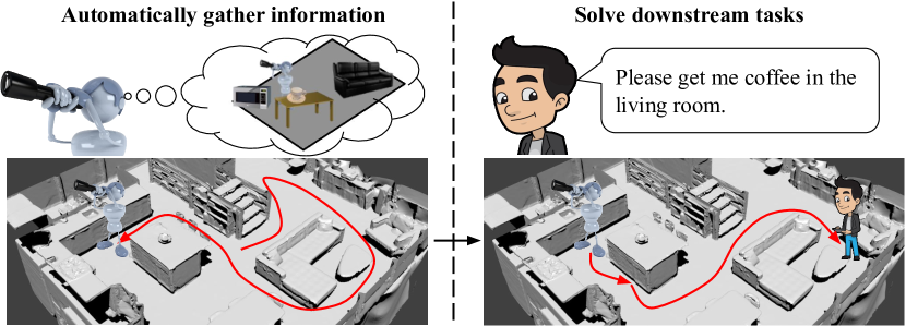
Intelligent exploration in 3D environments is important as it allows unsupervised preparation for future tasks. Embodied agents that have the ability to explore are flexible to deploy, since they can use knowledge about previously seen environments to quickly gather useful information in the new one, without having to rely on humans. This ability allows them to prepare for unspecified downstream tasks in the new environment. For example, a newly deployed home-robot could prepare itself by automatically discovering rooms, corridors, and objects in the house. After this exploration stage, it could quickly adapt to instructions such as “Bring coffee from the kitchen to Steve in the living room.” See Fig. 1.
A variety of exploration methods have been proposed both in the reinforcement learning and computer vision literature. They employ ideas like curiosity [59, 49, 11], novelty [65, 9, 57], coverage [16, 15], and reconstruction [33, 54, 61] to overcome sparse rewards [9, 49, 11, 57] or learn task-agnostic policies that generalize to new tasks [33, 16, 54]. In this study, we consider algorithms designed to handle complex photorealistic indoor environments where a mobile agent observes the world through its camera’s field of view and can exploit common semantic priors from previously seen environments (as opposed to exploration in randomly generated mazes or Atari games).
How do different exploration algorithms work for different types of environments and downstream tasks? Despite the growing literature on embodied visual exploration, it has been hard to analyze what works when and why. This difficulty is due to several reasons. First, prior work evaluates on different simulation environments such as SUN360 [54, 61], ModelNet [54, 61], VizDoom [49, 57], SUNCG [16], DeepMindLab [57], and Matterport3D [15]. Second, prior work uses different baselines with varying implementations, architectures, and reinforcement learning algorithms. Finally, exploration methods have been evaluated from different perspectives such as overcoming sparse rewards [49, 11], pixelwise reconstruction of environments [33, 53, 54, 61], area covered in the environment [16, 15], object interactions [50, 27], or as an information gathering phase to solve downstream tasks such as navigation [16], recognition [33, 54, 61], or pose estimation [54]. Due to this lack of standardization, it is hard to compare any two methods in the literature.
This paper presents a unified view of exploration algorithms for visually rich 3D environments, and a common evaluation framework to understand their strengths and weaknesses. First, we formally define the exploration task. Next, we provide a taxonomy of exploration approaches and sample representative methods for evaluation. We evaluate these methods and several baselines on common ground: two well-established 3D datasets [2, 14] and a state-of-the-art neural architecture [16]. Unlike navigation and recognition, which have clear-cut success measures, exploration is more open-ended. Hence, we quantify exploration quality along multiple meaningful dimensions such as mapping, robustness to sensor noise, and relevance for different downstream tasks. Finally, by systematically evaluating different exploration methods using this benchmark, we highlight their strengths and weaknesses, and we identify key factors for learning good exploration policies.
Our main contribution is the first unified and systematic empirical study of exploration paradigms on 3D environments. In the spirit of recent influential studies in other domains [20, 42, 24, 45, 44], we aim first and foremost to provide a reliable, unbiased, and thorough view of the state of the art that can be a reference to the field moving forward. To facilitate this, we introduce technical improvements to shore up existing approaches, and we propose new baselines and performance metrics. We will publicly release all code to standardize the development and evaluation of exploration algorithms.
2 Empirical study framework
First, we define a framework for systematically studying different exploration algorithms. We formulate exploration as a sequential information-gathering task: at each time step, the agent takes as input the current view and history of accumulated views, updates its internal model of the environment (e.g., a spatial memory or map), and selects the next action (i.e., camera motion) to maximize the information it gathers about the environment. How the latter is defined is specific to the exploration algorithm, as we will detail in Sec. 3. This process may be formalized as a finite-horizon partially observed Markov decision process (POMDP). In the next few sections, we describe the POMDP formulation, the 3D simulators used to realize it, the policy architecture that accounts for partial observability while taking actions, and the policy learning algorithm.
2.1 The exploration POMDP
We model exploration as a partially observed Markov decision process (POMDP) [41]. A POMDP can be represented as a tuple with state space , observation space , action space , state-conditioned observation distribution , transition distribution , reward function , initial state distribution , and discount factor . The agent is spawned at an initial state in an unknown environment. At time , the agent at state receives an observation , executes a camera motion action , receives a reward , and reaches state . The state representation is obtained using the history of observations , and is the agent’s policy. We assume a finite episode length .
The goal is to learn an optimal exploration policy that maximizes the expected cumulative sum of the discounted rewards over an episode:
| (1) |
where is a sequence of tuples generated by starting at and behaving according to policy at each time step. The reward function captures the method-specific incentive for exploration (see Sec. 3). Next, we concretely define the instantiation of the POMDP in terms of photorealistic 3D simulators.
2.2 Simulators for embodied perception
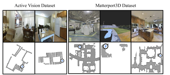
In order to standardize the experimentation pipeline, we use simulators built on top of two realistic 3D datasets: Active Vision Dataset [2] (AVD) and Matterport3D [14] (MP3D). See Fig. 2. There are several other valuable 3D assets in the community [72, 37, 6, 64]; we choose MP3D and AVD for this study due to their complementary attributes (see Tab. 1). We anticipate that the different facets of the two datasets will allow us to better elicit any differences in behavior between the paradigms we test.
| Properties | Active Vision Dataset [2] | Matterport3D [14] |
|---|---|---|
| View sampling | Discrete | Continuous |
| Size (average navigable space) | Small () | Large () |
| Train / val / test splits | 9 / 2 / 4 | 61 / 11 / 18 |
| Large scale data | No | Yes |
| Outdoor components | No | Yes |
| Clutter | Significant | Mild |
| Forward motion | 0.3 | 0.25 |
| Rotation angle |
The Active Vision Dataset (AVD) is a dataset of dense RGB-D scans from 15 unique indoor houses and office buildings [2]. We simulate embodied motion by converting the dataset into a connectivity graph with discrete points and moving along the edges of the graph (similar to [5]). Compared to Matterport3D, AVD environments are relatively smaller in size, fewer in number, and have noisy depth inputs and coarsely discretized movements. The coarse sampling of views in AVD prevents continuous simulation of camera motion, as the reconstructed meshes tend to have significant mesh defects. However, movement along discrete nodes placed approximately apart allows a realistic simulation for an embodied agent in cluttered home interiors, which are lacking in real estate photos or computer graphics datasets.
Matterport3D (MP3D) is a dataset of photorealistic 3D meshes from 90 indoor buildings [14]. The MP3D environments are generally larger in size, greater in quantity, and offer more finely discretized movements than AVD. Some MP3D environments contain outdoor components such as swimming pools, porches, and gardens which present unique challenges to exploration, as we will see in Sec. 5.3. We use the publicly available Habitat simulator [44], which provides fast simulation.
In these simulation environments, the state space consists of the agent’s position and orientation within the environment. The observation space consists of an RGB-D sensor, an odometer to track the camera position, and a bump sensor to detect collisions. We consider exploration under both idealized noise-free sensing and realistic noisy conditions. The action space is discrete and has three actions: move forward, turn left, and turn right. The motion values are given in Tab. 1.
We stress that though the agents we test are simulated robots, the 3D visual spaces in which we test them are real—they are comprised of real meshes captured from real images, not generated from models with computer graphics. While real robots do introduce challenges beyond perception, realistic simulations have the advantage of reproducibility and scaling agent experience, and hence are widely used today [4, 14, 18, 44, 58, 64, 72]. Furthermore, our experiments examine the effects of noisy odometry and noisy occupancy in these environments. Finally, recent work shows promising results transferring from simulated environments (including Matterport3D) to real-world exploration and navigation, supporting simulators as a meaningful testbed for our benchmark [15, 34].
2.3 Policy architecture
In order to successfully explore an unknown environment, the agent needs to keep track of where it is currently located, how much of the environment has been explored, what information was contained in the explored regions, and what are the potentially unexplored parts of the environment. We select a state-of-the-art policy architecture that is well-suited to these objectives and has shown successful exploration in partially-observed and visually rich 3D environments [16].
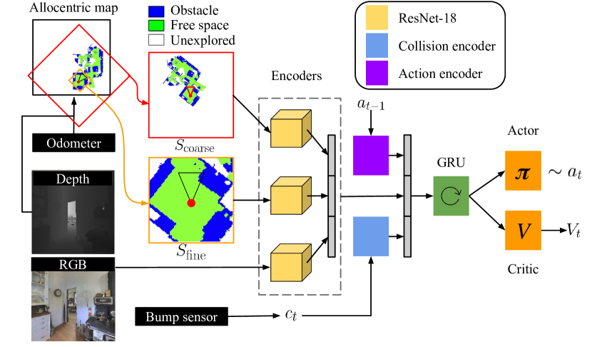
The agent receives sensory readings from an RGB-D sensor, an odometer that measures the motion resulting from the past action, and a bump sensor that detects collisions resulting from past actions. The policy architecture consists of three parts: (1) spatial memory, (2) temporal memory, and (3) an actor-critic model (see Fig. 3). We elaborate on these parts in the following.
Spatial memory
As the agent explores an environment, it needs to keep track of what areas are explored and where the obstacles are present, and then decide where to navigate next in order to explore further. This is done by maintaining a top-down occupancy map that represents free, occupied, and unexplored regions in the environment (see Fig. 3). The map is built geometrically by using depth inputs to estimate the occupied and free regions based on pixel heights at a given location, and then registering them to the allocentric map based on the agent’s pose.
Let be the sequence of depth maps and pose estimates of the agent up to time . The agent’s pose at time is expressed as , with representing the agent’s camera rotation and translation in the world coordinates. Let the agent initially start at the origin of the map, i.e., , and let be the intrinsic camera matrix, which is assumed to be provided. Each pixel in the depth map can then be projected to the 3D point cloud as follows:
| (2) |
where is the total number of pixels in . This gives us the set of points representing all observed points during exploration. We discretize the top-down view of the environment into discrete 2D cells of size and classify each cell into three categories—free space, obstacle, and unexplored space—as follows:
| (3) |
where is the height of point , and are height thresholds in meters used to determine occupancy, and is the set of points present within cell with heights less than . This gives us the agent’s allocentric spatial memory specifying which regions are free space, obstacle, and unexplored space. Based on the allocentric memory and the agent’s current pose, egocentric crops at two resolutions and are provided to the next stages, where and are measured in meters.
Temporal memory
While the spatial memory purely encodes geometric information, the agent needs to additionally store other textural and semantic cues in the environment over time. This is done via a temporal memory that jointly encodes all sensor inputs and aggregates them over time.
The RGB and the coarse and fine occupancy maps are encoded as 128-D feature vectors via independent pre-trained ResNet-18 [29] models, then concatenated and fused into a 512-D feature vector using a fully connected (FC) layer. The previous action and binary collision signal are encoded as learned 32-D embeddings. The encoded image, action, and collision features are concatenated, and then fused using an FC layer to obtain a 512-D feature vector at each time-step. This is temporally aggregated using a Gated Recurrent Unit (GRU) [17] with one hidden-layer and 512-D hidden-state.
Actor critic model
Given the encoded information from the sensors over time, the agent needs to decide what action to execute in the environment during exploration. We learn the exploration policy via the actor-critic paradigm, which consists of an actor to sample actions and a critic to model the value of the agent’s current state [67]. The actor and critic are each modeled using two fully connected layers. The actor outputs the action probabilities for the policy at each time-step, and the critic predicts a scalar state value.
This policy architecture facilitates long-term information storage and effective planning by exploiting geometric and semantic cues in the environment. Unlike traditional SLAM, such a learned spatio-temporal memory—popular in recent embodied perception approaches [25, 30, 16, 15]—allows the agent to leverage both statistical visual patterns learned from training environments as well as geometry to extrapolate what it learns to novel environments.
2.4 Policy learning algorithm
In order to train the policy architecture, we adapt current methods [18, 19, 16] and divide the learning into two stages: (1) imitation learning, and (2) fine-tuning with reinforcement learning. The imitation learning stage is intended to reduce sample complexity for the reinforcement learning stage by offering a better initialization of the policy.
Imitation learning:
We first pre-train the exploration policy via imitation learning [10, 23]. We generate synthetic expert trajectories by treating the environment as a graph of connected nodes and exploiting this connectivity graph to greedily explore the environment (discussed more in Sec. 4.1). Given these trajectories, we minimize the cross-entropy error between the predicted and expert actions at each step. Additionally, we diversify the training trajectories by sampling actions from the agent’s policy with probability , instead of exclusively following the expert trajectories. We use inflection weighting to prevent the policy from simply repeating the previous action [70]. The perturbation is varied from to during the course of training with a constant increase of after every updates. For AVD, , , . For MP3D, , , . These values were obtained through validation on the validation environments.
Reinforcement learning:
We then fine-tune the policy with the RL training objective using Proximal Policy Optimization (PPO) [60]. The PPO surrogate objective is:
| (4) |
where are the policy parameters, is the probability ratio of the updated and old policies at time , is the advantage estimate, and is the clipping factor. We optimize for this objective using the Adam optimizer [36]. More implementation details can be found in Appendix 0.C.
Given this empirical study framework consisting of standardized task definitions, simulators, policy architecture, and learning algorithm, we can plug in different reward functions to train different exploration agents, as we describe next.
3 Taxonomy of exploration paradigms
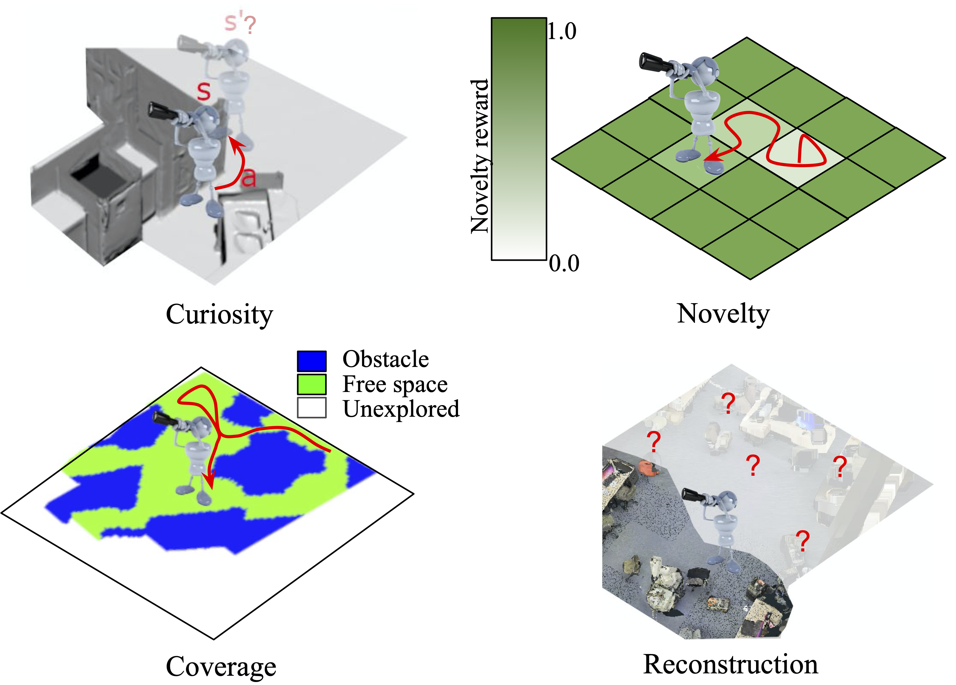
We now present a taxonomy for exploration algorithms in the literature. We identify four core paradigms (see Fig. 4):
(1) curiosity: encourages visiting states where the agent’s uncertainty is high.
(2) novelty: encourages visiting states that are unvisited.
(3) coverage: encourages visiting states that reveal unseen areas in the environment.
(4) reconstruction: encourages visiting states that lead to better prediction of unseen states.
Each paradigm can be viewed as a particular reward function in the POMDP. In the following, we review their key ideas and related work, and choose representative methods for benchmarking that capture the essence of each paradigm.
3.1 Curiosity
In the curiosity paradigm, the agent is encouraged to visit states where its predictive model of the environment is uncertain [59, 47, 40, 49]. See Fig. 4, top left. We focus on the dynamics-based formulation of curiosity, which was shown to perform well on large-scale scenarios [49, 11]. The agent learns a forward-dynamics model that predicts the effect of an action on the agent’s state, i.e, . Then, the curiosity reward at each time step is:
| (5) |
The forward-dynamics model is trained online to minimize the loss in forward-dynamics prediction: . Thus, the curiosity reward encourages the agent to move to newer states once its forward-dynamics predictions on the past states are accurate. We adapt the curiosity formulation from [49] for our experiments. Instead of using image features as the state representation for the forward dynamics model, we use the GRU hidden state in Sec. 2.3 as we found it helped alleviate the partial observability. We follow recommended practices such as using PPO for policy optimization, reward normalization, observation normalization, and using feature normalization in the CNN [11].
Past work on curiosity-driven exploration
The forward-dynamics based formulation of curiosity uses an inverse-dynamics prediction loss to learn features that ignore parts of the environment not useful for dynamics prediction [49]. Stable features kept fixed during policy learning are found to perform better in many cases [11]. Further variants of curiosity aim to overcome the “noisy-TV” problem where the curiosity agent fixates on parts of the environment where stochasticity is a function of its actions [11, 12, 51]. For example, if the agent has access to a TV remote that allows it to randomly change channels, it does that repeatedly to accumulate rewards. Due to the inherently random nature of the transitions, they can never be predicted accurately and always reward the agent. Random Network Distillation attempts to overcome this limitation by defining a fixed random neural network as the predictive function since it is a deterministic function of the inputs [12]. Exploration via Disagreement attempts to resolve the issue by learning an ensemble of forward-prediction models and using their disagreement as intrinsic motivation rather than the prediction error [51]. Curiosity is also demonstrated to work on physically realistic 3D simulators with the addition of a self-aware model that learns to anticipate errors in the agent’s predictions [27].
3.2 Novelty
While curiosity seeks hard-to-predict states, novelty seeks previously unvisited states [65, 9, 46, 68, 57]. See Fig. 4, top right. Each is assigned a visitation count . The novelty reward is inversely proportional to the square-root of visitation frequency at the current state:
| (6) |
For our experiments, we adapt the Grid Oracle method from [57]: we discretize the 3D environment into a 2D grid where each grid cell is considered to be a unique state, and assign rewards according to Eqn. 6. We define square grid cells of width in AVD and in MP3D, and consider all points within a grid cell to correspond to that state.
Past work on novelty-based exploration
Early methods on interval estimation or count-based exploration define a confidence interval over the optimal value function of the underlying Markov Decision Processes (MDP) and apply this idea to tabular RL settings [65]. More recent work extends this idea to function approximation settings by using the notion of pseudo-counts [9] combined with complex density models [46], or discretizing high-dimensional continuous spaces into discrete representations through hash functions [68], which facilitates a tabular RL setting. Rather than using dynamics prediction, episodic curiosity [57] rewards states that look dissimilar from previously visited ones, yielding a binary variant of Eqn. 6. We use the GridOracle from [57] as it was shown to explore successfully in a variety of settings.
3.3 Coverage
The coverage paradigm aims to observe as many things of interest as possible—typically the area seen in the environment [16, 15]. See Fig. 4, bottom left. Whereas novelty encourages explicitly visiting all locations, coverage encourages observing all of the environment. Note that the two are distinct: at any given location, how much and how far a robot can see varies depending on the surrounding 3D structures. The coverage approach from [16] learns RL policies that maximize area coverage. The area-coverage reward is:
| (7) |
where is the area covered by the agent till time (blue and green regions in Fig. 3). An agent maximizing area seen prioritizes those locations and viewing angles which provide high visibility of unseen parts of the environment.
While this is shown to work well on diverse environments [16], the agent is never rewarded for revisiting the same regions. In our experiments, we find that this leads to a specific form of reward sparsity in large environments (as we will highlight in Sec. 5.4). Consider the case where an agent starts exploring from the center of a very large building. After it explores one half of the building, there will be no learning signal for the agent to move back to the center in order to continue exploring the other half. Therefore, we incorporate ideas from the novelty reward to design a shaped version of coverage that addresses this limitation, which we call smooth-coverage:
| (8) |
where is the set of regions seen in the environment at time and is the number of times a region has been observed so far. Instead of only rewarding the agent for the first time it sees a region (as in Eq. 7), we reward the agent based on the number of times that region was observed. This allows the agent to navigate across less frequently visited regions to discover unexplored parts of the environment.
While we use area as our primary quantity of interest, this idea can more generally be exploited for learning to visit other interesting things such as objects (similar to the search task from [21]) and landmarks. See Appendix 0.D for comparative results.
Past work on coverage-based exploration
Recent work explores using novel architectures that better optimize the coverage objective. The area coverage objective is optimized through a combination of imitation and reinforcement learning to learn exploration policies that generalize well to novel environments [16]. A new hierarchical architecture combines classic-planning and learned controllers to successfully optimize the area coverage objective in a sample-efficient manner under realistic noise models [15]. Scene memory transformers propose an architecture based on transformers [69] that encode observations at each time-step into a feature space where self-attention is used to perform reasoning [21]. The model is shown to be successful on several tasks including area coverage and object class coverage (i.e., visiting as many object classes as possible). These architectural variants are orthogonal to our study since our primary goal is to explore the choice of reward function to facilitate exploration.
3.4 Reconstruction
Reconstruction-based methods [33, 53, 54, 61] use the objective of active observation completion [33] to learn exploration policies. The idea is to gather views that best facilitate the prediction of unseen viewpoints in the environment. See Fig. 4, bottom right. The reconstruction reward scores the quality of the predicted outputs:
| (9) |
where is a set of true “query” views at camera poses in the environment, is the set of view reconstructions generated by the agent after time steps, and is a distance function. Whereas curiosity rewards views that are individually surprising, reconstruction rewards views that bolster the agent’s correct hallucination of all other views.
Prior attempts at exploration with reconstruction are limited to pixelwise reconstructions on panoramas and CAD models, where is on pixels. To scale the idea to 3D environments, we propose a novel adaptation that predicts concepts present in unobserved views rather than pixels, i.e., a form of semantic reconstruction. This reformulation requires the agent to predict whether, say, an instance of a “door” concept is present at some query location, rather than reconstruct the door pixelwise as in [33, 54].
We automatically discover these visual concepts from the training environments, which has the advantage of not relying on supervised object detectors or semantic annotations. Specifically, we sample views uniformly from training environments and cluster them into discrete concepts using -means applied to ResNet-50 features. Each cluster centroid is a concept and may be semantic (doors, pillars) or geometric (arches, corners).
Then, we reward the agent for acquiring views that help it accurately predict the dominant concepts in all query views sampled from a uniform grid of locations in each environment. Let denote the ResNet-50 feature for the -th query view. We define its true “reconstructing” concepts to be the nearest cluster centroids to , and assign equal probability to those concepts. The agent has a multilabel classifier that takes a query pose as input—not the view —and returns , the posteriors for each concept being present in . The distance in Eqn (9) is the KL-divergence between the true concept distribution and the agent’s inferred distribution , summed over all . The reward thus encourages reducing the prediction error in reconstructing the true concepts. In practice, we shape the reward function to be the reduction in the KL divergence over time (as opposed to the absolute KL divergence value) as this leads to better performance; see Appendix 0.A.2.
Past work on reconstruction-based exploration
The original reconstruction-based exploration approach [33] rewards exploration that permits more accurate pixelwise reconstructions of scenes and objects. It was shown that the resulting exploratory policies accelerate recognition tasks. Sidekick policy learning [53] exploits full state information available only at training time to accelerate training and learn better policies. Broader transferability of exploration policies on the tasks of recognition, volume estimation, and other tasks are demonstrated in [54], and the quality of pixelwise reconstructions are enhanced using a pix2pix [31] model. Architectural improvements based on a spatial memory and foveated viewpoints yield high-quality reconstructions with lower viewing costs [61].
Reconstruction-based exploration approaches also relate to classical information-gain based exploration, where the goal is to explore in order to reduce the uncertainty in the agent’s model of the world [13, 63, 66]. The action entropy control strategy in [13] explores in order to maximize the information gained about the agent’s belief state when the certainty of the optimal action is low. In [63], the agent is encouraged to take actions that minimize the uncertainty in pose estimation and mapping. Optimal Bayesian exploration is used to maximize the agent’s knowledge about a parameterized world model [66]. Our proposed formulation that reconstructs in a discrete concept space can be viewed as a form of information-gain based exploration. The high-dimensional image-state representation is projected to a smaller concept space, and the reward function encourages maximizing the the information gain between the agent’s knowledge of the concepts present in the environment and the states visited by the agent.
4 Exploration evaluation framework
Having defined the taxonomy of exploration algorithms, we now define baselines and metrics to evaluate them.
4.1 Baseline methods
Heuristic baselines: Aside from the learned paradigms introduced above, we also evaluate four non-learned heuristics for exploration:
(1) random-actions [54, 44] samples from a uniform distribution over all actions.
(2) forward-action [44] always samples the forward action.
(3) forward-action+ samples the forward action unless a collision occurs, in which case, it turns left.
(4) frontier-exploration [73] uses the egocentric map from Fig. 3 and iteratively visits the frontiers, i.e., the edges between free and unexplored spaces (see Appendix 0.E). The frontier approach is closely related to area-coverage, but depends on hand-crafted heuristics and may be vulnerable to noisy sensors and actuators.
Oracle graph exploration: As an upper bound on exploration performance, we also include an oracle model. It cheats by exploiting the underlying graph structure in the environment (which reveals reachability and obstacles) to visit a sequence of sampled target locations via the true shortest paths. In contrast, all methods we benchmark are not given this graph, and must discover it through exploration. We define three oracles that visit (1) randomly sampled locations, (2) landmark views (see Sec. 4.2), and (3) objects within the environment.
Imitation learning: We imitate the oracle trajectories to get three imitation variants, one for each oracle above. Whereas the oracles assume full observability and therefore are not viable exploration approaches, these imitation learning baselines are viable, assuming disjoint training data with full observability is available.
Tab. 2 lists the assumptions on information availability made by the different approaches. Methods requiring less information are more flexible. While we assume access to the full environment during training, there is ongoing work [9, 46, 57] on relaxing this assumption.
| Training / Testing | ||||
| GT depth | GT pose | GT objects | GT state | |
| random-actions | - / No | - / No | - / No | - / No |
| forward-action(+) | - / No | - / No | - / No | - / No |
| imitation-X | Yes / Yes* | Yes / Yes* | Yes / No | Yes / No |
| curiosity | Yes / Yes* | Yes / Yes* | No / No | No / No |
| novelty | Yes / Yes* | Yes / Yes* | No / No | Yes / No |
| frontier-exploration | - / Yes | - / Yes | - / No | - / No |
| coverage | Yes / Yes* | Yes / Yes* | Yes / No | No / No |
| oracle | No / No | No / No | Yes / Yes | Yes / Yes |
4.2 Evaluation metrics
A good exploration method visits interesting locations and collects information that is useful for a variety of downstream tasks. Different methods may be better suited for different tasks. For example, a method optimizing for area coverage may not interact sufficiently with objects, leading to poor performance on object-centric tasks. We measure exploration performance with two families of metrics:
(1) Visiting interesting things.
These metrics quantify the extent to which the agent visits things of interest such as area [16, 73, 15, 21], objects [21, 27], and landmarks. The area visited metric measures the amount of area covered in . For the objects visited metric, we use the object annotations provided by both AVD and MP3D to measure how many objects are visited during exploration. We consider an object to be visited if the agent is close to it and the object is unoccluded within its field of view. For the landmarks visited metric, we mine a set of “landmark” viewpoints from the environment which contain distinctive visual components that do not appear elsewhere in that environment, e.g., a colorful painting or a decorated fireplace.222See Appendix 0.G for more details on how landmarks are mined. The exact visitation criteria for both objects and landmarks are given in Appendix 0.B. Together, these visitation metrics capture the different levels of semantic and geometric reasoning that an agent may need to perform in the environment. To account for varying environment sizes and content, we normalize each metric into by dividing by the best oracle score on each episode.
(2) Downstream task transfer.
These metrics directly evaluate exploration’s impact on downstream tasks. The setup is as follows: an exploration agent is given a time budget of to explore the environment, after which the information gathered must be utilized to solve a task within the same environment. More efficient exploration algorithms gather better information and are expected to have higher task performance.
We consider three tasks from the literature that ask fundamental, yet diverse questions: (i) PointNav: how to quickly navigate from point A to point B? (ii) view localization: where was this photo taken? and (iii) reconstruction: what can I expect to see at point B?
In PointNav, the agent is respawned at the original starting point after exploration, and given a navigation goal relative to its position [4, 58]. The agent must use its map acquired during exploration to navigate to the goal within a maximum of time steps. Intuitively, for efficient navigation, an exploration algorithm needs to explore potential dead ends in the environment that may cause planning failure. We use an A* planner that navigates using the spatial occupancy map built during exploration [28]. While other navigation algorithms are possible, A* is a consistent and lightweight means to isolate the impact of the exploration models. We evaluate using the success rate normalized by the path length (SPL) [4].
In view localization, the agent is presented with images sampled from distinct landmark viewpoints (introduced previously in Sec. 4.2) and must localize them relative to its starting location [54]. This task captures the agent’s model of the overall layout, e.g., “where would you need to go to see this view?”. While PointNav requires planning a path to a point target around obstacles, view localization requires locating a visual target. We measure localization accuracy by the pose-success rate (PSR), the fraction of views localized within mm of their ground truth pose.
In reconstruction, the agent is presented with uniformly spread query locations, and must predict the set of concepts present at each location [33, 54, 61] (cf. Sec. 3.4). This can be viewed as the inverse problem of view localization: the agent has to predict views given locations. Performance is measured using Precision between the agent’s predicted concepts and the ground truth.
For each task, we define a standard pipeline that uses the exploration experience to solve the task in Appendix A. We do not fine-tune exploration policies for downstream tasks since we treat them as independent evaluation metrics.
Together, the proposed metrics capture both geometric and semantic aspects of spatial sensing. For example, the area-visited metric reflects 2D SLAM (occupancy) and the reconstruction task metric measures semantic SLAM, where the goal is to map concepts present in the environment.
5 Experiments
We next present the results on various exploration metrics.
Implementation details
All policies are trained for on AVD/MP3D for 2000 episode batches. We sample episodes on AVD/MP3D uniformly from all test environments. For navigation, we define difficult test episodes by selecting challenging pairs of start-goal positions on AVD/MP3D. They are selected such that the agent’s navigation would be inefficient unless the environment was already well explored prior to navigation (see Appendix 0.F). More implementation details are provided in Appendix 0.C.
5.1 Results on exploration metrics
We compare the performance of different paradigms on visitation metrics and downstream task transfer in AVD and MP3D. Since the two datasets exhibit a variety of contrasting properties by design (see Sec. 2.2), we may expect to see corresponding differences in the results. For brevity, only the best of the three oracle and imitation variants on each metric are reported. Note that coverage here corresponds to smooth-coverage, which we found to consistently outperform area-coverage.
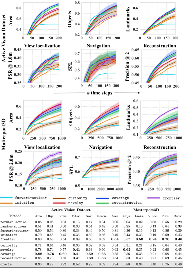
Fig. 5 shows the results on both datasets, and Fig. 7 shows example exploration episodes. These results are for the ideal noise-free odometry case. We will separately analyze the impact of noisy odometry in the next section. We see two clear trends emerging:
In AVD, both coverage and reconstruction clearly outperform novelty. While novelty assigns equal rewards to all locations in the environment, coverage and reconstruction prioritize viewpoints that are useful for quickly covering area and concepts, respectively. This significantly improves exploration performance in the small, cluttered rooms of AVD. However, we do not observe a similar effect in MP3D as novelty outperforms both these methods. This is due to two reasons. First, since the rooms in MP3D are generally open and large, the advantage of prioritizing the viewpoints is smaller than in AVD. Second, the reward functions of coverage and reconstruction are inherently sparser than novelty. The reconstruction method does not reward the agent for reconstructing concepts that it already reconstructed in the past (reduction in KL divergence is smaller). The original area-coverage method does not reward the agent for seeing the same area more than once. As we will show in an ablation in Sec. 5.4, the improved smooth-coverage method bridges the gap between area-coverage and novelty to a good extent.
The performance of curiosity is worse than that of other paradigms on both datasets, likely due to the significant partial observability that is characteristic of these visually rich 3D environments. Its performance deteriorates further on MP3D environments which tend to be much larger, and it even underperforms the imitation baseline. curiosity needs a good state representation that accounts for partial observability to learn a good forward dynamics model that leads to better reward estimates. This is naturally harder in larger MP3D environments. As we will show in ablations in Sec. 5.4, the memory architecture that we use here is better for curiosity than using only image features. It is possible that incorporating better memory architectures could boost the performance even further.
Good baselines are essential for measuring progress on any benchmark. Our proposed baseline imitation is significantly better than the standard baselines random-actions, forward-action, and forward-action+ used in prior work [54, 44, 16]. While learned methods generally outperform these baselines, frontier-exploration outperforms most learned methods on MP3D. Since fronter-exploration relies on clean depth inputs with a perfectly registered map, it underperforms in AVD since the depth inputs are naturally noisy (see Sec. 2). As we will show in the next section, a similar phenomenon can also be in observed in MP3D where noisy sensor inputs deteriorate its performance, echoing past findings [16].
In Fig. 5, we see that the navigation performance for all methods in MP3D are inferior to the state-of-the-art performance reported in standard navigation benchmarks on MP3D [44] due to the increased difficulty of the test episodes. Additionally, we observe that the trends on the navigation metric on both AVD and MP3D differ from the other metrics. The gaps between different methods are reduced, imitation closely competes with other paradigms, and much larger values of are required to improve the performance in MP3D. This hints at the inherent difficulty of exploring well to navigate: efficient navigation requires exploration agents to uncover potential obstacles that reduce path planning efficiency. Notably, existing exploration methods do not incorporate such priors into their rewards.
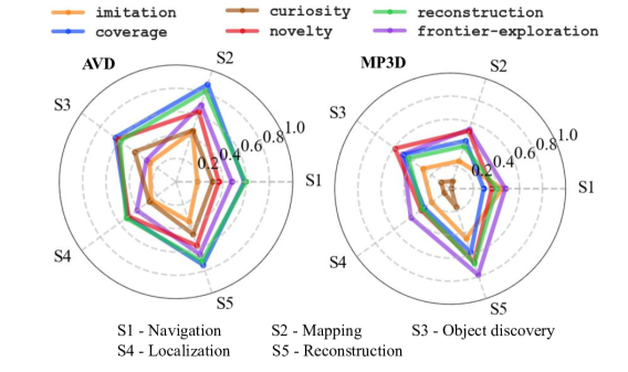
The radar plots in Fig. 5.1 concisely summarize the results thus far along five skills: Mapping, Navigation, Object discovery, Localization, and Reconstruction. The metrics corresponding to these skills are area visited, pointnav SPL, objects visited, view localization PSR, and reconstruction precision@2, respectively. The metrics are normalized to [0, 1] where 0 and 1 represent the performance of random-actions and oracle, respectively. In each case, a method’s performance on the metric is normalized as follows:
| (10) |
As we can see in Fig. 5.1, coverage dominates the other paradigms on most skills, closely followed by reconstruction in AVD. In the larger MP3D environments, different methods are stronger on different skills. For example, novelty performs best on object discovery, frontier-exploration dominates on localization and reconstruction, and both dominate on mapping. This highlights the need for diverse evaluation metrics for exploration.
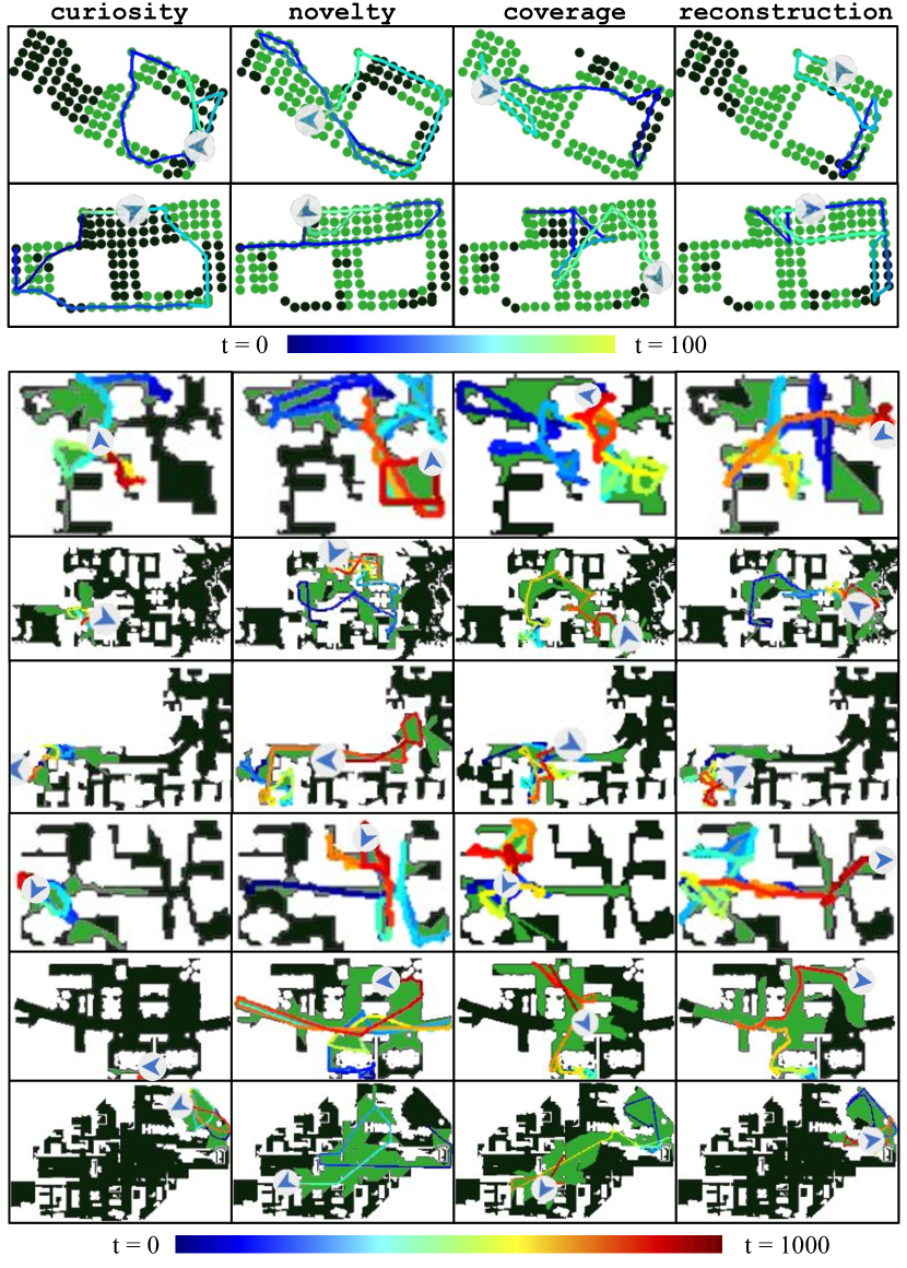
Fig. 7 shows qualitative examples of exploration in AVD and MP3D for the four paradigms. Better methods cover larger areas of the environment during exploration.
5.2 Impact of sensor noise on exploration
In the previous section, we evaluated the exploration performance of various algorithms under noise-free odometry. Now, we evaluate the impact of sensor noise during exploration, specifically the noise arising from two sources: (1) the occupancy map, and (2) odometer readings. We perform our experiments in MP3D as it contains larger and more diverse testing environments.
Impact of noisy occupancy estimation
Noisy occupancy maps can result from mesh defects, noisy depth, and incorrect estimates of affordances from the height-based estimation method (see Sec. 2.3) [52]. This noise occurs naturally and is not explicitly simulated, meaning all results reported thus far are where the methods do experience noisy occupancy. The noise-free case can be simulated by directly extracting occupancy maps from the navigability information stored in the simulator, instead of estimating it from visual cues. We characterize the impact of this noise through the noise robustness coefficient (NRC), the ratio of the area visited333We select area visited because it is a simple metric that does not require additional semantic annotations. by an agent with the original depth-based occupancy maps (noisy) and ground-truth occupancy maps obtained from the simulator (noise-free). Larger NRC indicates better adaptation to noisy test conditions.
Tab. 3 shows the exact values of area visited with noisy and noise-free occupancy, and the corresponding NRC values. As we can see, learned approaches have an NRC close to , indicating that they perform similarly under both conditions. 444The NRC values may be larger than for learned methods. This is due to domain differences between the inferred occupancy used in training and the GT occupancy used in testing. However, a purely geometric approach like frontier-exploration has a much lower NRC (). Since the simulation conditions in MP3D are generally noise-free and the noise levels are low, frontier-exploration still gets better absolute performance than most approaches. In contrast, the depth maps in AVD lead to persistent noise in the occupancy estimates, which causes frontier-exploration to do worse than other approaches there (see Fig. 5).
| Effect of incorrectly estimated occupancy maps on exploration | |||
|---|---|---|---|
| Method | Inferred occupancy | GT occupancy | NRC |
| imitation | 0.452 | 0.386 | 1.17 |
| frontier-exploration | 0.579 | 0.748 | 0.77 |
| coverage | 0.522 | 0.508 | 1.03 |
| novelty | 0.622 | 0.599 | 1.04 |
| curiosity | 0.317 | 0.317 | 1.00 |
| reconstruction | 0.510 | 0.503 | 1.01 |
Impact of noisy odometry
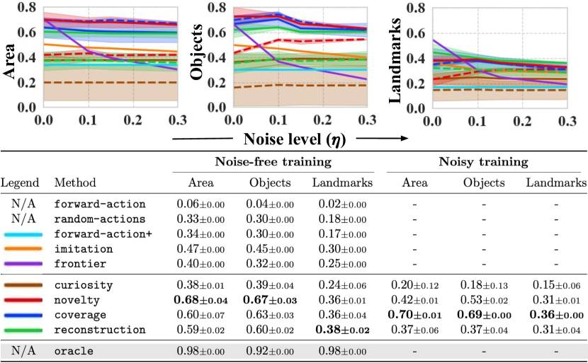
Next, we measure the impact of a noisy odometer during the exploration evaluation phase. Noisy odometry leads to incorrect registration of local point clouds, estimated from the depth map to the allocentric map (see Sec. 2.3). This noise affects the spatial memory of the agent and effectively leads to noisy occupancy inputs to the exploration policy. Note that this is different from the noisy occupancy maps case where we measure the impact of per-frame noise in occupancy. Here, we are more interested in the noise occurring in the long-term map registration.
We consider two variants: noisy training and noise-free training. Adding noise to odometry during training additionally affects the reward functions used for policy learning. For curiosity, the features used for forward-dynamics prediction are noisy, since they include the noisy occupancy estimates. For novelty, the state visitation counts will be noisier since the agent is unsure of its position in the global coordinates. For coverage, this directly affects the measure of coverage used in the reward function since coverage measurements rely on accurate odometry. For reconstruction, this affects the pose inputs associated with each observation obtained during exploration, which may lead to worse predictions.
Following past work [16], we use a truncated Gaussian noise model whose standard deviation is proportional to the action magnitudes (see Tab. 1). Specifically, at each time step, we sample a random perturbation from a truncated Gaussian with mean 0, standard deviation , and a truncation width of on either sides of the mean. Here, is the noise level and is the action magnitude. The agent estimates its current position by summing up the odometer readings over time. Therefore, the noise gets accumulated over time leading to increasingly large deviations in the agent’s pose estimates.
Fig. 8 compares the four paradigms along with baselines. When trained under noise-free conditions, the learned methods generalize relatively well to different testing noise levels, despite not being exposed to noisy inputs during training. Interestingly, their relative trends are consistent across the different noise levels during testing. However, the performance of frontier-exploration deteriorates rapidly as the noise level increases. For noisy training conditions, we set the noise level as . While coverage remains robust to noisy training conditions, the exploration performance deteriorates for most learning-based methods when compared to the noise-free training conditions. This is expected since the reward function becomes less reliable under noise-free training conditions. Nevertheless, the learning-based approaches outperform frontier-exploration at higher noise levels.
5.3 Scale factors that influence performance
We now analyze how scaling factors affect exploration quality.
How does dataset size affect learning?
First we analyze how the exploration performance varies with the training dataset size, i.e., the number of unique training environments in MP3D. We select novelty and smooth-coverage as they are the top performers on MP3D. We additionally select area-coverage to compare its behavior with smooth-coverage. We train agents on 3 random subsets of MP3D environments and measure their exploration performance at on the full MP3D test set.
Fig. 9 shows the results. Interestingly, all agents achieve very good performance with only 10 training environments. We observe the benefit of well-shaped rewards provided by novelty and smooth-coverage, which decay exponentially based on the visitation/observation frequency. While their performances improve with the number of environments, it saturates quickly for area-coverage. There is gradual but steady improvement in the performance from 10 environments to the full training set, suggesting that these approaches might continue to benefit from significantly larger training environment sets.

How does environment size affect exploration?
Next we select the top five methods on MP3D and measure their performance as a function of testing environment size (see Fig. 10). First, we group test episodes based on area visited by the best oracle. Within each group, we report the of episodes in which each method ranks in the top 3 out of 5. The larger this value, the better the method is on those environments. The novelty and coverage approaches are robust and perform well on most environment sizes. The reconstruction approach also competes well, especially in larger environments. However, frontier-exploration struggles in large MP3D environments as they tend to contain mesh defects where the agent gets stuck. Please see Appendix 0.H for qualitative examples.

5.4 Ablation studies
In the foregoing experiments, we have proposed two changes to implementations of prior work: (1) using a smoother variant of the area-coverage reward function proposed in [16], and (2) using the feature representation from a memory architecture for curiosity as opposed to image representations as done in [49, 11, 16]. We now evaluate the effect of these changes on exploration performance.
How do smoother rewards affect exploration?
As we discussed in Sec. 3.3, the formulation of area-coverage leads to specific forms of reward sparsity. We addressed this by proposing the smooth-coverage method. We now evaluate the impact of making this change across different metrics and datasets. In Tab. 4, we compare the two coverage approaches on all six metrics on AVD and MP3D. As we can see, smooth-coverage leads to consistent improvements across most metrics on AVD and across the visitation metrics in MP3D.
| Active Vision Dataset | ||||||
|---|---|---|---|---|---|---|
| Method | Area | Objects | Landmarks | View Local. | Navigation | Reconstruction |
| area-coverage | ||||||
| smooth-coverage | ||||||
| Matterport3D | ||||||
| Method | Area | Objects | Landmarks | View Local. | Navigation | Reconstruction |
| area-coverage | ||||||
| smooth-coverage | ||||||
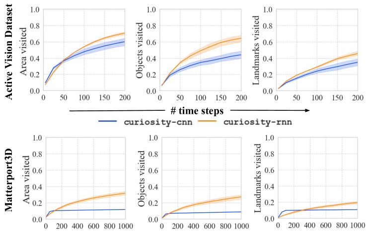
How do memory-based representations influence curiosity-driven exploration?
As discussed in Sec. 5.1, curiosity requires good feature representations that account for partial observability in large 3D environments. Using better memory architectures for learning can improve the performance by maintaining longer-term state representations. In Fig. 11, we compare the performance between the spatio-temporal memory (spatial map + RNN) based representation that we use (curiosity-rnn) and the version used in [16] where pre-trained ImageNet features were used as the feature representation (curiosity-cnn). As we can see, using the RNN feature representation leads to significant improvements on all visitation metrics. In fact, curiosity-cnn fails to learn any meaningful behaviors in MP3D. Despite the improvement seen here, the overall performance of curiosity is significantly worse than the other paradigms. Curiosity-driven exploration may therefore benefit from having even better memory architectures. In addition, having a large number of parallel environments is critical for training curiosity-based agents [11]. This is not practical in our case where we use large-scale 3D environments that have significantly higher computational and data constraints than simpler 2D scenarios.
6 Conclusions
We considered the problem of visual exploration in 3D environments. Prior work presents results on varying experimental conditions, making it hard to analyze what works when. Motivated by this, we proposed a novel benchmark for consistently evaluating exploration algorithms under common experimental conditions: policy architecture, 3D environments, learning algorithm, and diverse evaluation metrics. We then presented a comparative study of four popular exploration paradigms on this standardized benchmark.
To enable this study, we introduced new metrics and baselines, and we improved upon some existing approaches to scale well to 3D environments. Specifically, we extend the ideas from reconstruction-based exploration scene exploration approaches to work on general 3D environments. We also introduced a new coverage reward function that improves upon the existing area-coverage method. Our analysis provides a comprehensive view of the state of the art and each paradigm’s strengths and weaknesses.
To recap some of our key findings:
-
•
In the small and cluttered environments from Active Vision Dataset, the coverage and reconstruction methods are the strongest paradigms as they prioritize selecting views that maximally increase information.
-
•
In the large and open environments from Matterport3D, novelty and smooth-coverage approaches are the strongest paradigms as they have smoother reward functions which are easier to optimize in large environments.
-
•
In the diverse Matterport3D testing environments, different approaches tend to dominate on different skills, highlighting the need for diverse evaluation metrics.
-
•
The performance trends among learned approaches remain consistent in noise-free and noisy test conditions, whereas a purely geometric approach like frontier-exploration tends to deteriorate rapidly in the presence of sensor noise.
-
•
Our proposed smooth-coverage method improves over a prior coverage approach by using a smoother reward function that eases optimization and leads to consistently better performance on a variety of conditions.
-
•
Our proposed adaptation of reconstruction successfully explores 3D environments and competes closely with the best methods on most settings.
-
•
Improved memory architectures may be the key to scaling curiosity-driven exploration to visually-rich 3D environments under extreme partial observability.
-
•
An easy-to-implement heuristic imitation significantly outperform baselines typically employed, and can serve as a better baseline for future research.
We hope that our study serves as a useful starting point and a reliable benchmark for future research in embodied visual exploration. Code, data, and models are publicly available.
Acknowledgements
UT Austin is supported in part by DARPA Lifelong Learning Machines and the GCP Research Credits Program.
References
- [1] Aloimonos, J., Weiss, I., Bandyopadhyay, A.: Active vision. International Journal of Computer Vision (1988)
- [2] Ammirato, P., Poirson, P., Park, E., Kosecka, J., Berg, A.: A dataset for developing and benchmarking active vision. In: ICRA (2016)
- [3] Anderson, P., Chang, A., Chaplot, D.S., Dosovitskiy, A., Gupta, S., Koltun, V., Kosecka, J., Malik, J., Mottaghi, R., Savva, M., Zamir, A.R.: On evaluation of embodied navigation agents. arXiv preprint arXiv:1807.06757 (2018)
- [4] Anderson, P., Chang, A., Chaplot, D.S., Dosovitskiy, A., Gupta, S., Koltun, V., Kosecka, J., Malik, J., Mottaghi, R., Savva, M., et al.: On evaluation of embodied navigation agents. arXiv preprint arXiv:1807.06757 (2018)
- [5] Anderson, P., Wu, Q., Teney, D., Bruce, J., Johnson, M., Sünderhauf, N., Reid, I., Gould, S., van den Hengel, A.: Vision-and-language navigation: Interpreting visually-grounded navigation instructions in real environments. In: Proceedings of the IEEE Conference on Computer Vision and Pattern Recognition (CVPR) (2018)
- [6] Armeni, I., Sax, A., Zamir, A.R., Savarese, S.: Joint 2D-3D-Semantic Data for Indoor Scene Understanding. ArXiv e-prints (2017)
- [7] Bajcsy, R.: Active perception. Proceedings of the IEEE (1988)
- [8] Ballard, D.H.: Animate vision. Artificial intelligence (1991)
- [9] Bellemare, M., Srinivasan, S., Ostrovski, G., Schaul, T., Saxton, D., Munos, R.: Unifying count-based exploration and intrinsic motivation. In: Advances in Neural Information Processing Systems (2016)
- [10] Bojarski, M., Del Testa, D., Dworakowski, D., Firner, B., Flepp, B., Goyal, P., Jackel, L.D., Monfort, M., Muller, U., Zhang, J., et al.: End to end learning for self-driving cars. arXiv preprint arXiv:1604.07316 (2016)
- [11] Burda, Y., Edwards, H., Pathak, D., Storkey, A., Darrell, T., Efros, A.A.: Large-scale study of curiosity-driven learning. In: arXiv:1808.04355 (2018)
- [12] Burda, Y., Edwards, H., Storkey, A., Klimov, O.: Exploration by random network distillation. arXiv preprint arXiv:1810.12894 (2018)
- [13] Cassandra, A.R., Kaelbling, L.P., Kurien, J.A.: Acting under uncertainty: Discrete bayesian models for mobile-robot navigation. In: Proceedings of IEEE/RSJ International Conference on Intelligent Robots and Systems. IROS’96, vol. 2, pp. 963–972. IEEE (1996)
- [14] Chang, A., Dai, A., Funkhouser, T., , Nießner, M., Savva, M., Song, S., Zeng, A., Zhang, Y.: Matterport3d: Learning from rgb-d data in indoor environments. In: Proceedings of the International Conference on 3D Vision (3DV) (2017). MatterPort3D dataset license available at: http://kaldir.vc.in.tum.de/matterport/MP_TOS.pdf.
- [15] Chaplot, D.S., Gupta, S., Gupta, A., Salakhutdinov, R.: Modular visual navigation using active neural mapping
- [16] Chen, T., Gupta, S., Gupta, A.: Learning exploration policies for navigation. In: International Conference on Learning Representations (2019). URL https://openreview.net/pdf?id=SyMWn05F7
- [17] Chung, J., Gulcehre, C., Cho, K., Bengio, Y.: Empirical evaluation of gated recurrent neural networks on sequence modeling. arXiv preprint arXiv:1412.3555 (2014)
- [18] Das, A., Datta, S., Gkioxari, G., Lee, S., Parikh, D., Batra, D.: Embodied Question Answering. In: Proceedings of the IEEE Conference on Computer Vision and Pattern Recognition (CVPR) (2018)
- [19] Das, A., Gkioxari, G., Lee, S., Parikh, D., Batra, D.: Neural modular control for embodied question answering. In: Conference on Robot Learning, pp. 53–62 (2018)
- [20] Duan, Y., Chen, X., Houthooft, R., Schulman, J., Abbeel, P.: Benchmarking deep reinforcement learning for continuous control. In: International Conference on Machine Learning, pp. 1329–1338 (2016)
- [21] Fang, K., Toshev, A., Fei-Fei, L., Savarese, S.: Scene memory transformer for embodied agents in long-horizon tasks. In: Proceedings of the IEEE Conference on Computer Vision and Pattern Recognition, pp. 538–547 (2019)
- [22] Fischler, M.A., Bolles, R.C.: Random sample consensus: a paradigm for model fitting with applications to image analysis and automated cartography. Communications of the ACM 24(6), 381–395 (1981)
- [23] Giusti, A., Guzzi, J., Cireşan, D.C., He, F.L., Rodríguez, J.P., Fontana, F., Faessler, M., Forster, C., Schmidhuber, J., Di Caro, G., et al.: A machine learning approach to visual perception of forest trails for mobile robots. IEEE Robotics and Automation Letters (2016)
- [24] Goyal, P., Mahajan, D., Gupta, A., Misra, I.: Scaling and benchmarking self-supervised visual representation learning. arXiv preprint arXiv:1905.01235 (2019)
- [25] Gupta, S., Davidson, J., Levine, S., Sukthankar, R., Malik, J.: Cognitive mapping and planning for visual navigation. In: Proceedings of the IEEE Conference on Computer Vision and Pattern Recognition, pp. 2616–2625 (2017)
- [26] Gupta, S., Fouhey, D., Levine, S., Malik, J.: Unifying map and landmark based representations for visual navigation. arXiv preprint arXiv:1712.08125 (2017)
- [27] Haber, N., Mrowca, D., Fei-Fei, L., Yamins, D.L.: Learning to play with intrinsically-motivated self-aware agents. arXiv preprint arXiv:1802.07442 (2018)
- [28] Hart, P.E., Nilsson, N.J., Raphael, B.: A formal basis for the heuristic determination of minimum cost paths. IEEE transactions on Systems Science and Cybernetics 4(2), 100–107 (1968)
- [29] He, K., Zhang, X., Ren, S., Sun, J.: Deep residual learning for image recognition. In: Proceedings of the IEEE conference on computer vision and pattern recognition, pp. 770–778 (2016)
- [30] Henriques, J.F., Vedaldi, A.: Mapnet: An allocentric spatial memory for mapping environments. In: proceedings of the IEEE Conference on Computer Vision and Pattern Recognition, pp. 8476–8484 (2018)
- [31] Isola, P., Zhu, J.Y., Zhou, T., Efros, A.A.: Image-to-image translation with conditional adversarial networks. arxiv (2016)
- [32] Jayaraman, D., Grauman, K.: End-to-end policy learning for active visual categorization. IEEE Transactions on Pattern Analysis and Machine Intelligence (2018)
- [33] Jayaraman, D., Grauman, K.: Learning to look around: Intelligently exploring unseen environments for unknown tasks. In: Computer Vision and Pattern Recognition, 2018 IEEE Conference on (2018)
- [34] Kadian, A., Truong, J., Gokaslan, A., Clegg, A., Wijmans, E., Lee, S., Savva, M., Chernova, S., Batra, D.: Are we making real progress in simulated environments? measuring the sim2real gap in embodied visual navigation. arXiv preprint arXiv:1912.06321 (2019)
- [35] Kay, W., Carreira, J., Simonyan, K., Zhang, B., Hillier, C., Vijayanarasimhan, S., Viola, F., Green, T., Back, T., Natsev, P., et al.: The kinetics human action video dataset. arXiv preprint arXiv:1705.06950 (2017)
- [36] Kingma, D.P., Ba, J.: Adam: A method for stochastic optimization. arXiv preprint arXiv:1412.6980 (2014)
- [37] Kolve, E., Mottaghi, R., Han, W., VanderBilt, E., Weihs, L., Herrasti, A., Gordon, D., Zhu, Y., Gupta, A., Farhadi, A.: AI2-THOR: An Interactive 3D Environment for Visual AI. arXiv (2017)
- [38] Kostrikov, I.: Pytorch implementations of reinforcement learning algorithms. https://github.com/ikostrikov/pytorch-a2c-ppo-acktr-gail (2018)
- [39] Lin, T.Y., Maire, M., Belongie, S., Hays, J., Perona, P., Ramanan, D., Dollár, P., Zitnick, C.L.: Microsoft coco: Common objects in context. In: European Conference on Computer Vision (2014)
- [40] Lopes, M., Lang, T., Toussaint, M., Oudeyer, P.Y.: Exploration in model-based reinforcement learning by empirically estimating learning progress. In: Advances in neural information processing systems, pp. 206–214 (2012)
- [41] Lovejoy, W.S.: A survey of algorithmic methods for partially observed markov decision processes. Annals of Operations Research 28(1), 47–65 (1991)
- [42] Mahmood, A.R., Korenkevych, D., Vasan, G., Ma, W., Bergstra, J.: Benchmarking reinforcement learning algorithms on real-world robots. In: Conference on Robot Learning, pp. 561–591 (2018)
- [43] Malmir, M., Sikka, K., Forster, D., Movellan, J., Cottrell, G.W.: Deep Q-learning for active recognition of GERMS. In: BMVC (2015)
- [44] Manolis Savva*, Abhishek Kadian*, Oleksandr Maksymets*, Zhao, Y., Wijmans, E., Jain, B., Straub, J., Liu, J., Koltun, V., Malik, J., Parikh, D., Batra, D.: Habitat: A Platform for Embodied AI Research. In: Proceedings of the IEEE/CVF International Conference on Computer Vision (ICCV) (2019)
- [45] Mishkin, D., Dosovitskiy, A., Koltun, V.: Benchmarking classic and learned navigation in complex 3d environments. arXiv preprint arXiv:1901.10915 (2019)
- [46] Ostrovski, G., Bellemare, M.G., van den Oord, A., Munos, R.: Count-based exploration with neural density models. In: Proceedings of the 34th International Conference on Machine Learning-Volume 70, pp. 2721–2730. JMLR. org (2017)
- [47] Oudeyer, P.Y., Kaplan, F., Hafner, V.V.: Intrinsic motivation systems for autonomous mental development. IEEE transactions on evolutionary computation 11(2), 265–286 (2007)
- [48] Paszke, A., Gross, S., Chintala, S., Chanan, G., Yang, E., DeVito, Z., Lin, Z., Desmaison, A., Antiga, L., Lerer, A.: Automatic differentiation in PyTorch. In: NIPS Autodiff Workshop (2017)
- [49] Pathak, D., Agrawal, P., Efros, A.A., Darrell, T.: Curiosity-driven exploration by self-supervised prediction. In: International Conference on Machine Learning (2017)
- [50] Pathak, D., Gandhi, D., Gupta, A.: Beyond games: Bringing exploration to robots in real-world (2018)
- [51] Pathak, D., Gandhi, D., Gupta, A.: Self-supervised exploration via disagreement. arXiv preprint arXiv:1906.04161 (2019)
- [52] Qi, W., Mullapudi, R.T., Gupta, S., Ramanan, D.: Learning to move with affordance maps. arXiv preprint arXiv:2001.02364 (2020)
- [53] Ramakrishnan, S.K., Grauman, K.: Sidekick policy learning for active visual exploration. In: Proceedings of the European Conference on Computer Vision (ECCV), pp. 413–430 (2018)
- [54] Ramakrishnan, S.K., Jayaraman, D., Grauman, K.: Emergence of exploratory look-around behaviors through active observation completion. Science Robotics 4(30) (2019). DOI 10.1126/scirobotics.aaw6326. URL https://robotics.sciencemag.org/content/4/30/eaaw6326
- [55] Russakovsky, O., Deng, J., Su, H., Krause, J., Satheesh, S., Ma, S., Huang, Z., Karpathy, A., Khosla, A., Bernstein, M., Berg, A.C., Fei-Fei, L.: ImageNet Large Scale Visual Recognition Challenge. International Journal of Computer Vision (2015)
- [56] Savinov, N., Dosovitskiy, A., Koltun, V.: Semi-parametric topological memory for navigation. arXiv preprint arXiv:1803.00653 (2018)
- [57] Savinov, N., Raichuk, A., Marinier, R., Vincent, D., Pollefeys, M., Lillicrap, T., Gelly, S.: Episodic curiosity through reachability. arXiv preprint arXiv:1810.02274 (2018)
- [58] Savva, M., Chang, A.X., Dosovitskiy, A., Funkhouser, T., Koltun, V.: Minos: Multimodal indoor simulator for navigation in complex environments. arXiv preprint arXiv:1712.03931 (2017)
- [59] Schmidhuber, J.: Curious model-building control systems. In: Proc. international joint conference on neural networks, pp. 1458–1463 (1991)
- [60] Schulman, J., Wolski, F., Dhariwal, P., Radford, A., Klimov, O.: Proximal policy optimization algorithms. arXiv preprint arXiv:1707.06347 (2017)
- [61] Seifi, S., Tuytelaars, T.: Where to look next: Unsupervised active visual exploration on 360 deg input. arXiv preprint arXiv:1909.10304 (2019)
- [62] Soomro, K., Zamir, A.R., Shah, M.: Ucf101: A dataset of 101 human actions classes from videos in the wild. arXiv preprint arXiv:1212.0402 (2012)
- [63] Stachniss, C., Grisetti, G., Burgard, W.: Information gain-based exploration using rao-blackwellized particle filters.
- [64] Straub, J., Whelan, T., Ma, L., Chen, Y., Wijmans, E., Green, S., Engel, J.J., Mur-Artal, R., Ren, C., Verma, S., Clarkson, A., Yan, M., Budge, B., Yan, Y., Pan, X., Yon, J., Zou, Y., Leon, K., Carter, N., Briales, J., Gillingham, T., Mueggler, E., Pesqueira, L., Savva, M., Batra, D., Strasdat, H.M., Nardi, R.D., Goesele, M., Lovegrove, S., Newcombe, R.: The Replica dataset: A digital replica of indoor spaces. arXiv preprint arXiv:1906.05797 (2019)
- [65] Strehl, A.L., Littman, M.L.: An analysis of model-based interval estimation for markov decision processes. Journal of Computer and System Sciences 74(8), 1309–1331 (2008)
- [66] Sun, Y., Gomez, F., Schmidhuber, J.: Planning to be surprised: Optimal bayesian exploration in dynamic environments. In: International Conference on Artificial General Intelligence, pp. 41–51. Springer (2011)
- [67] Sutton, R.S., Barto, A.G.: Reinforcement learning: An introduction. MIT press (2018)
- [68] Tang, H., Houthooft, R., Foote, D., Stooke, A., Chen, O.X., Duan, Y., Schulman, J., DeTurck, F., Abbeel, P.: # exploration: A study of count-based exploration for deep reinforcement learning. In: Advances in neural information processing systems, pp. 2753–2762 (2017)
- [69] Vaswani, A., Shazeer, N., Parmar, N., Uszkoreit, J., Jones, L., Gomez, A.N., Kaiser, Ł., Polosukhin, I.: Attention is all you need. In: Advances in neural information processing systems, pp. 5998–6008 (2017)
- [70] Wijmans, E., Datta, S., Maksymets, O., Das, A., Gkioxari, G., Lee, S., Essa, I., Parikh, D., Batra, D.: Embodied question answering in photorealistic environments with point cloud perception. In: Proceedings of the IEEE Conference on Computer Vision and Pattern Recognition, pp. 6659–6668 (2019)
- [71] Wilkes, D., Tsotsos, J.K.: Active object recognition. In: Computer Vision and Pattern Recognition, 1992. IEEE Computer Society Conference on (1992)
- [72] Xia, F., Zamir, A.R., He, Z., Sax, A., Malik, J., Savarese, S.: Gibson env: Real-world perception for embodied agents. In: Proceedings of the IEEE Conference on Computer Vision and Pattern Recognition, pp. 9068–9079 (2018)
- [73] Yamauchi, B.: A frontier-based approach for autonomous exploration. (1997)
- [74] Yang, J., Ren, Z., Xu, M., Chen, X., Crandall, D., Parikh, D., Batra, D.: Embodied visual recognition. arXiv preprint arXiv:1904.04404 (2019)
- [75] Zamir, A.R., Wekel, T., Agrawal, P., Wei, C., Malik, J., Savarese, S.: Generic 3D representation via pose estimation and matching. In: European Conference on Computer Vision, pp. 535–553. Springer (2016)
- [76] Zhu, Y., Gordon, D., Kolve, E., Fox, D., Fei-Fei, L., Gupta, A., Mottaghi, R., Farhadi, A.: Visual Semantic Planning using Deep Successor Representations. In: Computer Vision, 2017 IEEE International Conference on (2017)
We provide additional information to support the text from the main paper. In particular, the appendix includes additional details regarding the following key topics:
Section 0.A: Downstream task transfer
Section 0.B: Criteria for visiting objects and landmarks
Section 0.C: Hyperparameters for learning exploration policies
Section 0.D: Comparative study of different coverage variants
Section 0.E: Frontier-exploration algorithm
Section 0.F: Generating difficult testing episodes for PointNav
Section 0.G: Automatically mining landmarks
Section 0.H: The factors influencing exploration performance
Appendix 0.A Downstream task transfer
We now elaborate on the three downstream tasks defined in Sec. 4.2: view localization, reconstruction, and PointNav navigation.
0.A.1 View localization pipeline
0.A.1.1 Problem Setup
An exploration agent is required to gather information from the environment that will allow it to localize key landmark views in the environment after exploration. Since the exploration agent does not know what views will be presented to it a priori, a general exploration policy that gathers useful information about the environment will perform best on this task.
More formally, the problem of view localization is as follows. The exploration agent is spawned at a random pose in some unknown environment, and is allowed to explore the environment for a time budget . Let be the set of observations the agent received and be the corresponding agent poses (relative to pose ). After exploration, a set of query views are sampled from query poses within the same environment and presented to the agent. The agent is then required to use the information gathered during exploration to predict . In practice, the agent is only required to predict the translation components of the pose, i.e., where represent the translation along the and axes from a top-down view of the environment. An agent that can successfully predict this has a good understanding of the layout of the environment as it can point to where a large set of views in the environment are sampled from. We next review the architecture for view localization. For the sake of simplicity, we consider the case of with denoting the query view and pose respectively.
0.A.1.2 View localization architecture
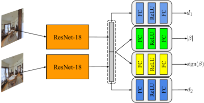
The architecture of our view localization model consists of four components (see Fig. 14).
Episodic Memory (E)
In order to store information over the course of a trajectory, we use an episodic memory E that stores the history of past observations and corresponding poses . For efficient storage, we only store image features vectors obtained from the pairwise pose predictor (P) and retrieval network (R) (as described in subsequent sections) in the memory.
Pairwise pose predictor (P)
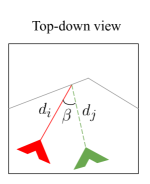
We train a pairwise pose predictor that takes in pairs of images that are visually similar (see next section), and predicts , where is the relative pose of in the egocentric coordinates of . The architecture is shown in Fig. 13. We follow a different parameterization of the pose prediction when compared to [75]. Instead of directly regressing , we first predict the distances to the points of focus (central pixel) for each image, and the baseline angle between the two viewpoints (see Fig. 12). The relative pose is then computed as follows:
This pose parameterization was more effective than directly regressing , especially when the data diversity was limited (eg. in AVD). To sample data for training the pose estimator, we opt for the sampling strategy from [75] (see Fig. 12). The prediction of is cast as independent regression problems with the MSE loss . The prediction of is split into two problems: predicting the baseline magnitude, and predicting the baseline sign. Baseline magnitude prediction is treated as a regression problem for AVD and as a 15-class classification problem for MP3D with corresponding MSE or cross entropy losses (. Baseline sign prediction is treated as a binary classification problem with a binary cross entropy loss . The overall loss function is:
| (11) |
Retrieval network (R)
We train a retrieval network R that, given a query image , can retrieve matching observations from E. Similar to [56], we use a siamese architecture consisting of a ResNet-18 feature extractor followed by a 2-layer MLP to predict the similarity score between images and . Since our goal is to retrieve observations that can be used by the pairwise pose predictor (P), the positive pairs are the same pairs used for training the pose predictor. Negative pairs are obtained by choosing random images that are far away from the current location. We use the binary cross entropy loss function to train the retrieval network.
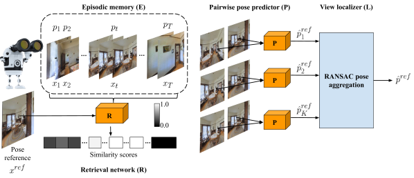
View localizer (L)
So far, we have a retrieval network R that retrieves observations that are similar to a query view , and a pairwise pose predictor P that predicts the relative pose between and each retrieved image. The goal of the view localizer (L) is to combine predictions made by P on individual retrievals given by R to obtain a robust estimate the final pose . The overall pipeline works as follows (see Fig. 14).
Similarity scores are computed between each in the episodic memory E and . The sequence of scores are temporally smoothed using a median filter to remove noisy predictions. After filtering out dissimilar images in the episodic memory, , we sample the top observations from with highest similarity scores. For each retrieved observation , we compute the relative pose , i.e., the predicted pose of in the egocentric coordinates of . We rotate and translate using , the real-world pose of , to get , the real-world pose of estimated from :
| (12) |
where are the rotation and translation components of . Given the set of individual predictions , we use RANSAC [22] to aggregate these predictions to arrive at a consistent estimate of .
0.A.1.3 Implementation details
For AVD, we restrict the baseline angle to lie in the range and depth values to lie in the range . We sample training, validation and testing pairs. While the number of samples are high, the diversity is quite limited since there are only 20 environments in total. For MP3D, we restrict the baseline angle to lie in the range and depth values to lie in the range . We sample training, validation and testing pairs. Both the pairwise pose predictor and retrieval network are trained (independently) using Adam optimizer with a learning rate of , weight decay of , batch size of . The ResNet-18 feature extractor is pretrained on ImageNet. The models are trained for 200 epochs and early stopping is performed using the loss on validation data. In case of AVD, the baseline magnitude predictor is a regression model that is trained using MSE loss. In MP3D, the baseline magnitude predictor is a 15-class classification model where each class represents a uniformly sampled bin in the range . The choice of classification vs. regression and the number of classes for predicting is made based on the validation performance. In both datasets, we use a median filter of size 3 with for the view localizer L. We sample the reference views from the set of landmark-views that we used in Sec. 4.2. Since these views are distinct and do not repeat in the environment, they are less ambiguous to localize.
0.A.2 Reconstruction pipeline

0.A.2.1 Problem setup: reconstruction
An exploration agent is required to gather information from the environment that will allow it to reconstruct views from arbitrarily sampled poses in the environment after exploration. Since the exploration agent does not know what poses will be presented to it a priori, a general exploration policy that gathers useful information about the environment will perform best on this task. This can be viewed as the inverse of the view localization problem where views are presented after exploration and their poses must be predicted.
Following the task setup from Sec. 3.4 in the main paper, the exploration agent is spawned at a random pose in some unknown environment and obtains the observations views and poses during exploration. After exploration, query poses are sampled from the same environment and the agent is required to reconstruct the corresponding views .
This reconstruction is performed in a concept space which is automatically discovered from the training environments. We sample views uniformly from the training environments and cluster their ResNet-50 features using K-means. The concepts are, therefore, the cluster centroids obtained after clustering image features. Each query location has a set of “reconstructing” concepts . These are determined by extracting the ResNet-50 features from and obtaining the nearest cluster centroids. We use a transformer [69] based architecture for predicting the concepts as described in Fig. 15. While this is similar to the policy architecture used in [21], we use the model to predict concepts present at a given location in the environment instead of learning a motion policy.
0.A.2.2 Loss function
Reconstruction in the concept space is treated as a multilabel classification problem. For a particular query view at a query pose , the reconstructing concepts are obtained by retrieving the top nearest neighbouring clusters in the image feature space. These clusters are treated as positive labels for and the rest are treated as negative labels. The ground-truth probability distribution assigned to consists of s for the negative labels and for the positive labels. Let be the posterior probabilites for each concept inferred by the model (see Fig. 15). Then, the loss is
where is the KL-divergence between the two distributions.
0.A.2.3 Reward function
The reconstruction method relies on rewards from a trained reconstruction model to learn an exploration policy. Note that the reconstruction model is not updated during policy learning. For each episode, a set of query poses and their views are sampled initially. This information is hidden from the exploration policy and does not affect the exploration directly. At time during an exploration episode, the agent will have obtained observations and . The reconstruction model uses to predict posteriors over the concepts for the different queries : . The reconstruction loss for each prediction is where is the reconstructing concept set for query . The reward is then computed as follows:
where the reward is provided to the agent after every steps. This reward is the reduction in the reconstruction loss over the past time-steps. The goal of the agent is to constantly reduce the reconstruction loss, and it is rewarded more for larger reductions.
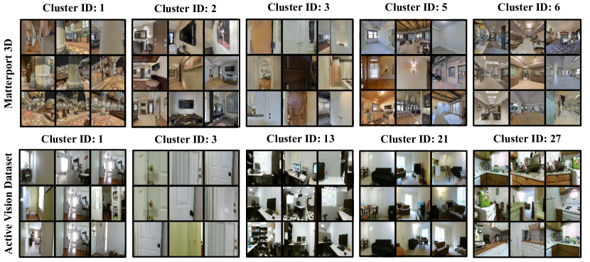
0.A.2.4 Implementation details
We sample clusters for AVD and clusters for MP3D based on the Elbow method which selects the , after which, the reduction in within-cluster separation saturates. Additionally, we manually inspect the clusters for different values of to ensure that they contain meaningful concepts (see Fig. 16).
In practice, we do not directly use the ResNet-50 image features as the output of the image encoder. We compute the similarity scores between the ResNet-50 features for a given and all the cluster centroids in . This gives an and dimensional vectors of similarities for AVD and MP3D, respectively which serves as the output of the image encoder. This design choice achieves two things, (1) it reduces computational complexity significantly as the number of clusters is much fewer than the ResNet-50 features (-D), and (2) it directly incorporates the information from cluster centroids into the reasoning process of the reconstruction, as the reasoning happens in the cluster similarity space rather than image feature space.
For training the reconstruction model, we sample exploration trajectories using the oracle exploration method. First, query views are sampled for each environment by defining a discrete grid of locations and sampling images from multiple heading angles at each valid location on the grid. For AVD, we use a grid cell distance of while sampling views from uniformly separated heading angles. For MP3D, we use a grid cell distance of while sampling views from uniformly separated heading angles. These values were selected to ensure a good spread of views, low redundancy in the views and adequate supervision (larger the grid cell distance, lesser the number of valid points). The model is trained on trajectories of length in AVD and in MP3D. We use nearest neighbors clusters as positives for both AVD and MP3D. For making the model more robust to the actual trajectory length, we also train on intermediate time-steps of the episode (after every steps in AVD and steps in MP3D). The optimization was performed using Adam optimizer with a learning rate of for AVD and for MP3D. We use 2 layers in both the transformer encoder and decoder with 2 attention heads each. For training the reconstruction exploration agent, we use for AVD and for MP3D.
0.A.3 Navigation pipeline
0.A.3.1 Problem setup
An exploration agent is required to gather information from the environment that will allow it to navigate to a given location after exploration.
More formally, the exploration agent is spawned at a random pose in some unknown environment, and is allowed to explore the environment for a time budget . Let be the set of depth observations the agent received and be the corresponding agent poses (relative to pose ). The depth observations along with the corresponding poses are used to build a 2D top-down occupancy map of the environment that indicates whether an location in the map is free, occupied, or unknown. After exploration, the agent is respawned at and is provided a target coordinate that it must navigate to within a budget of time , using the occupancy information gathered during exploration. After reaching the target, it is required to execute a STOP action indicating that it has successfully reached the target. Following past work on navigation [4, 44], the episode is considered to be a success only of the agent executed the stop action within a threshold geodesic distance from the target.
0.A.3.2 Navigation policy
We perform navigation using an A* planner that generates a path to the target at each time-step (See Algo. 1). The input to the policy consists of the egocentric occupancy map generated at the end of exploration and a target location on that map. The map consists of free, occupied and unexplored regions. converts this into a binary map by treating all free and unexplored regions as free space, and the occupied regions as obstacles. It also applies the morphology close operator to fill any holes in the binary map.
Next, the AStarPlanner uses the processed map to generate the shortest path from the current position to the target. If the policy has reached the target, then it returns STOP. Otherwise, if the path is successfully generated, the policy samples the next location on the path to navigate to () and selects an action to navigate to that target. is a simple rule-based action selector that moves forward if the agent is already facing the target, otherwise rotates left / right to face . However, if the path does not exist, the policy samples a random action. This condition is typically reached if ProcessMap blocks narrow paths to the target or assigns the agent’s position as an obstacle while closing holes.
0.A.3.3 Implementation details
We use a publicly available A* implementation: https://github.com/hjweide/a-star. We vary for benchmarking and set for AVD, MP3D. for AVD, MP3D. The value is larger for AVD since the environment is discrete, and a threshold of is satisfied only when the agent is one-step away from the target.
The map is an egocentric crop of the allocentric map generated during exploration. For AVD, we freeze the map after exploration, i.e., do not update the map based on observations received during the navigation phase. Therefore, the agent is required to have successfully discovered a path to the target during exploration (eventhough it does not know the target during exploration). This type of evaluation generally fails for MP3D since the floor-plans are very large and it is generally not possible for an exploration agent to discover the full floor plan within the restricted time-budget. Therefore, we permit online updates to during exploration. This means that the role of exploration in MP3D is to not necessarily discover a path to the target, instead, it is used to rule out certain regions of the environment that may cause planning failure, which would reduce the navigation efficiency.
Appendix 0.B Criteria for visiting objects and landmarks
We highlight the exact success criteria for what counts as visiting an object or landmark.
0.B.1 Visiting objects
AVD
The object instances in AVD [2] are annotated as follows: If an object is visible in an image, the bounding box and the instance ID are listed. A particular object instance is considered to be visited if it is annotated in the current image, the distance to the object is lesser than , and the bounding box area is larger than 70 squared pixels (approximately of an image). We keep the bounding box size threshold low since many of the object instances in AVD are very small objects555Examples of AVD object instances: https://www.cs.unc.edu/~ammirato/active_vision_dataset_website/get_data.html, and we primarily rely on visibility and the agent’s proximity to the object to determine visitation.
MP3D
The objects in MP3D [14] are annotated with center-coordinates in 3D space along with their extents specified as (width, height, depth). As stated in Sec. 4.2 in the main paper, to determine object visitation, we check if the agent is close to the object, has the object within its field of view, and if the object is not occluded. While it is also possible to arrive at similar visitation criteria by rendering semantic segmentations of the scene at each time step, we refrain from doing that as it typically requires larger memory to load semantic meshes and slows down rendering significantly. See Fig. 0.B.1 for the exact criteria. The values for this evaluation metric were determined upon manual inspection on training environments.
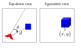
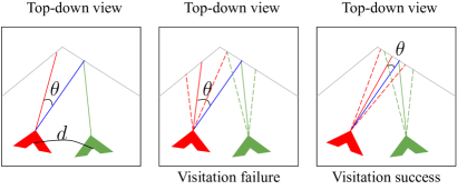
0.B.2 Visiting landmarks
The criteria for visiting landmarks differs from that of visiting objects as the goal here is to match a particular pose in the environment rather than be close to some location and have it within the agent’s field of view. Specifically, the goal is to look at the same things that the landmarks are looking at. See Fig. 0.B.1.
Appendix 0.C Hyperparameters for learning exploration policies
| AVD | MP3D | |
| Optimization | ||
| Optimizer | Adam | Adam |
| Learning rate | 0.00001 - 0.001 | 0.00001 - 0.001 |
| parallel actors | 32 | 8 |
| PPO mini-batches | 4 | 2 |
| PPO epochs | 4 | 4 |
| Training episode length | 200 | 500 |
| GRU history length | 50 | 100 |
| training steps (in millions) | 12.8 | 8 |
| Spatial memory | ||
| Map bin size | 0.05m | 0.1m |
| 0.3m | 0.5m | |
| 1.8m | 2.0m | |
| 10.0m | 20.0m | |
| 3.0m | 4.0m | |
| Reward scaling factors for different methods | ||
| Method | AVD | MP3D |
| curiosity | 0.001 | 0.0001 |
| novelty | 0.1 | 0.1 |
| smooth-coverage | 0.3 | 0.3 |
| reconstruction | 0.1 | 1.0 |
| area-coverage | 0.01 | 0.001 |
| random-views-coverage | 1.0 | 0.3 |
| landmarks-coverage | 1.0 | 1.0 |
| objects-coverage | 1.0 | 0.3 |
We expand on the implementation details provided in Sec. 5 from the main paper. We use PyTorch [48] and a publicly available codebase for PPO [38] for all our experiments. The hyperparameters for training different exploration algorithms are shown in Tab. 5. The optimization and spatial memory hyperparameters are kept fixed across different exploration algorithms. The primary factor that varies across methods is the reward scale. For MP3D, the models are trained on 4 Titan V GPUs and typically take 1-2 days for training. For AVD, the models are trained on 1 Titan V GPU and typically take 1 day to train.
Next, we compare our curiosity implementation with the one given in [11]. For training our curiosity policy, we use the forward-dynamics architecture proposed in [11] which consists of four MLP residual blocks. We use the GRU hidden state from the policy as our feature representation to account for partial observability. As recommended in [11], we do not backpropagate the gradients from the forward dynamics model to the feature representation to have relatively stable features. However, since the policy is updated, the features are not fixed during training (as suggested in [11]). Nevertheless, we found that it was more important to use memory-based features that account for partial observability, than to use stable image features that are frozen (see Fig. 11 in the main paper). We additionally use PPO, advantage normalization, reward normalization, feature normalization, and observation normalization following the practical considerations suggested in [11]. We are limited to using only 8 parallel actors due to computational and memory constraints.
Appendix 0.D Comparative study of different coverage variants
While we use area as our primary quantity of interest for coverage in the main paper, we extend this idea can more generally for learning to visit other interesting things such as objects (similar to the search task from [21]) and landmarks (see Sec 4.2 from the main paper). The coverage reward consists of the increment in some observed quantity of interest:
| (13) |
where is the quantity of interesting things (e.g., object) visited by time . Apart from area coverage (regular and smooth), we also consider objects and landmarks for , where the agent is reward based on the corresponding visitation metric from Sec. 4.2 in the main paper.
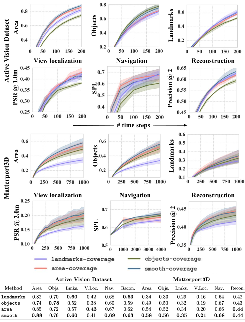
For each of the visitation metrics, we have one method that is optimized for doing well on that metric. For example, area-coverage optimizes for area visited, objects-coverage optimizes for objects visited, etc. As expected, on AVD we generally observe that the method optimized for a particular metric typically does better than most methods on that metric. However, on MP3D, we find that smooth-coverage and area-coverage dominate on most metrics. This shift in the trend is likely due to optimization difficulties caused by reward sparsity: landmarks and objects occur more sparsely in the large MP3D environments. Objects tend to occur more frequently in the environment than landmarks, and this is reflected in the performance as objects-coverage generally performs better. For this reason, we use smooth-coverage as the standard coverage method in the main paper.
Appendix 0.E Frontier-based exploration algorithm
We briefly describe the frontier-exploration baseline in Sec. 4.1 in the main paper. Here, we provide a detailed description of the algorithm along with the pseudo-code.
We implement a variant of the frontier-based exploration algorithm from [73] as shown in Algo. 2. The core structure of the algorithm is similar to the navigation policy used in Algo. 1. The key difference here is that the target is assigned by the algorithm itself.
DetectFrontiers()
Given the egocentric occupancy map of the environment, frontiers are detected. Frontiers are defined as the edges between free and unexplored regions in the map. In our case, we detect these edges and group them into contours using the contour detection algorithm from OpenCV. “frontiers” is the list of these contours representing different frontiers in the environment.
SampleTarget()
We sort the frontiers based on their lengths since longer contours represent potentially larger areas to uncover. We then randomly sample one of the three longest frontiers, and sample a random point within this contour to get .
UpdateMap()
We update the map based on observations received while navigating to . Once we sample a frontier target , we use a navigation policy (see Algo. 1 in the main paper) to navigate to the target. Since the occupancy maps can be noisy, we add two simple heuristics to make frontier-based exploration more robust. First, we keep track of the number of times planning to fails. This can happen if the map that is updated during exploration reveals that it is not possible to reach . Second, we keep track of the total time spent on navigating to . Depending on the map updates during exploration, certain targets may be very far away from the agent’s current position since the geodesic distance changes based on the revealed obstacles. If planning fails more than times or the time spent reaching crosses , then we sampled a new frontier target.
We use for both AVD, MP3D and for AVD and MP3D respectively. Preliminary analysis showed that the algorithm was relatively robust to different values of .
Appendix 0.F Generating difficult testing episodes for PointNav
In the implementation details provided in Sec. 5 of the main paper, we mentioned that we generate difficult test episodes for navigation. Here, we describe the rationale behind selecting difficult episodes and show some examples. In order to generate difficult navigation episodes, we ask the following question:
| How difficult would it be for an agent that has not explored the environment to reach the target? |
An agent that has not explored the environment would assume the entire environment is free and plan accordingly. When this assumption fails, i.e., a region that was expected to be free space is blocked, the navigation agent has to most likely reverse course and find a different path (re-plan). As newer obstacles are discovered along the planned shortest paths, navigation efficiency reduces as more re-planning is required. Therefore, an exploration agent that uses the exploration time budget to discover these obstacles a priori is expected to have higher navigation efficiency. We select start and goal points for navigation by manually inspecting floor-plans and identifying candidate (start, goal) locations that will likely require good exploration for efficient navigation. See Fig. 20 for some examples on MP3D. We use the same idea to generate episodes for AVD.
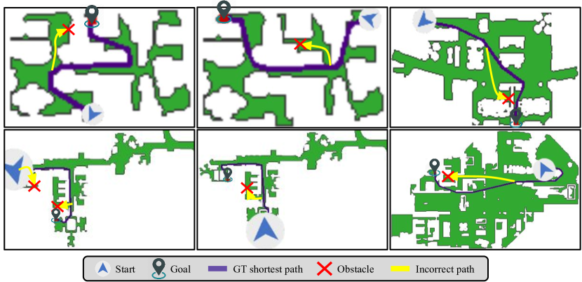
Appendix 0.G Automatically mining landmarks
In Sec. 4.2 from the main paper, we briefly motivated what landmarks are and how they are used for learning an exploration policy. Here, we explain how these landmarks are mined automatically from training data.
We define landmarks to be visually distinct parts of the environment, i.e., similar looking viewpoints do not occur in any other spatially distinct part of the environment. To extract such viewpoints from the environment, we sample large number of randomly selected viewpoints from each environment. For each viewpoint, we extract features from a visual similarity prediction network (see Sec. A.1 in the main paper) and cluster the features using K-Means. Visually similar view-points are clustered together due to the embedding learned by the similarity network. We then sort the clusters based on the intra-cluster variance in the (x, y, z) positions and select clusters with low variance. These clusters include viewpoints which do not have similar views in any other part of the environment, i.e., they are visually and spatially distinct. In indoor environments, these typically include distinct objects such as bicycles, mirrors and jackets, and also more abstract concepts such as kitchens, bedrooms and study areas (see Fig. 21 for examples).
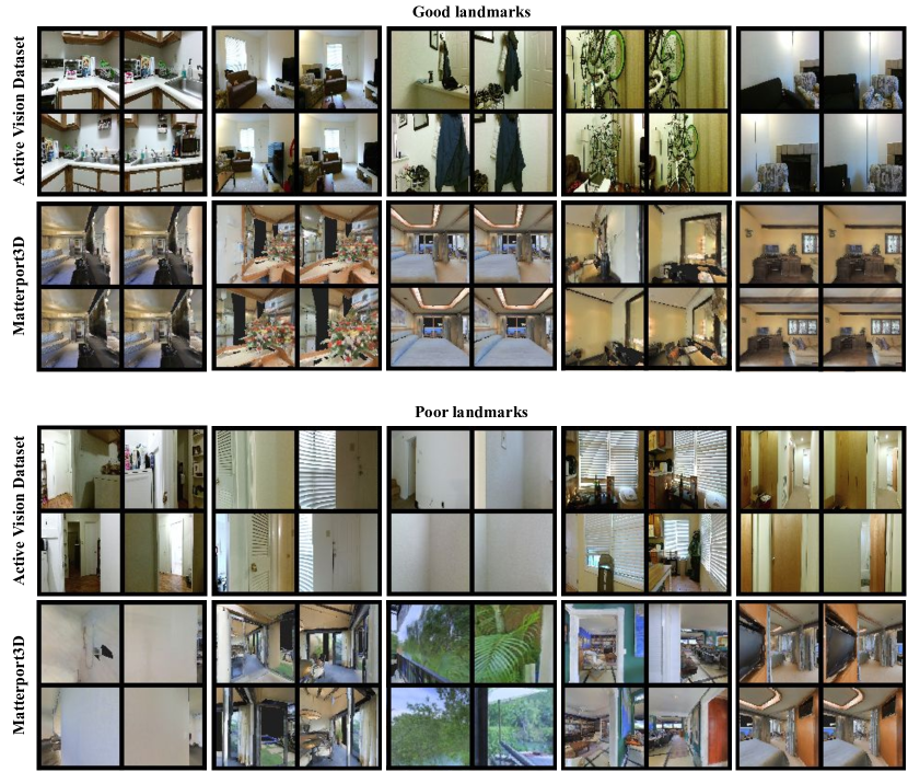
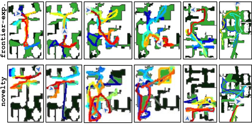
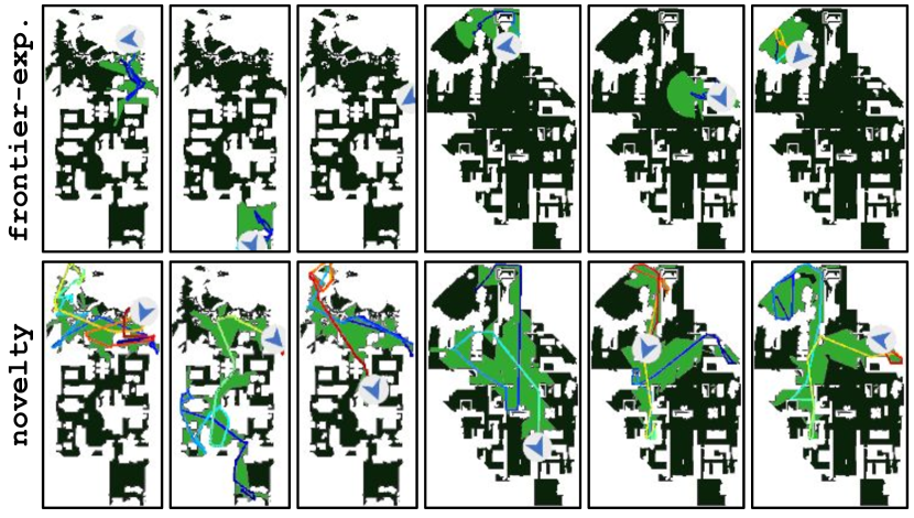
Appendix 0.H Factors influencing performance
In Sec. 5.3 from the main paper, we briefly discussed two different factors that affect quality of exploration, specifically, the number of training environments and the size of testing environments. Here, we provide qualitative examples of success and failure cases of frontier-exploration in the noise-free case on Matterport3D. We additionally analyze the impact of using imitation learning as a pre-training strategy for learning exploration staretgy.
0.H.1 Influence of testing environment size
As discussed in Sec. 5.3 in the main paper, novelty perform well on most environments. While frontier-exploration performs very well in small environments, it struggles in large MP3D environments. This is due to mesh defects present in the scans of large environments where the frontier agent gets stuck. Here, we show qualitative examples where frontier-exploration succeeds in small environments (see Fig. 0.G), and fails in large environments (see Fig. 0.G). For each example, we also show the exploration trajectories of novelty to serve as a reference because it succeeds on a wide variety of cases (see Fig. 10 from the main paper).
0.H.2 Influence of imitation-based pre-training
In Sec. 2.4 from the main paper, we mentioned that we pre-train policies with imitation learning before the reinforcement learning stage. Here, we evaluate the impact of doing so. See Fig. 24.
We train a few sample methods on both AVD and MP3D with, and without the imitation learning stage on three different random seeds. We then evaluate their exploration performance on 100 AVD episodes and 90 MP3D episodes as a function of the number of training episodes. Except in the case of novelty in MP3D, pre-training policies using imitation does not seem to improve performance or speed up convergence. While it is possible that expert trajectories gathered from humans (as opposed to synthetically generated) could lead to better performance, we reserve such analyses for future work.
