METHOD OF X-RAY DIFFRACTION
DATA PROCESSING FOR MULTIPHASE
MATERIALS WITH LOW PHASE CONTENTS

Abstract

Amorphous, glass, and glass-ceramic materials practically always include a significant number (more than eight) of crystalline phases, with the contents of the latter ranging from a few wt.% to several hundredths or tenths of wt.%.  The study of such materials using the method of X-ray phase analysis faces difficulties, when determining the phase structure.  In this work, we will develop a method for the analysis of the diffraction patterns of such materials, when diffraction patterns include X-ray lines, whose intensities are at the noise level.  The identification of lines is based on the search for correlations between the experimental and test lines and the verification of the coincidence making use of statistical methods (computer statistics).  The method is tested on the specimens of $\alpha$-quartz, which are often used as standard ones, and applied to analyze lava-like fuel-containing materials from the destroyed Chornobyl NPP Unit 4.  It is shown that the developed technique allows X-ray lines to be identified, if the contents of separate phases is not less than 0.1 wt.%.  The method also significantly enhances a capability to determine the phase contents quantitatively on the basis of lines with low intensities.

1 Introduction

As a result of the accident at the Chornobyl NPP, the main part of the nuclear fuel has spread over the premises of Unit 4 in the form of a melt.  These lava-like fuel-containing materials (LFCMs) include the main part of radionuclides of the spent fuel and, therefore, determine the nuclear, radiation, and environmental safety of the complex “New Safe Confinement – Shelter Object” [1].  In order to predict a change in the state of fuel-containing materials with time, it is necessary to know their structural parameters, including their type, size, and the contents of crystalline phases [2].

When applying the X-ray phase analysis to them, it was found that, firstly, the LLFCM specimens, in addition to glass on the basis of the silicon, uranium, aluminum, and zirconium oxides, contain also many (more than eight) crystalline phases; secondly, since the contents of those phases in the material are very low (from a few wt.% to several hundredths or tenths of wt.%), the intensities of a many hypothetically possible reflections (X-ray lines) from them are at the noise level; and thirdly, the number of such low-intensity reflections becomes extremely large: up to one or two hundred reflections [3].  The application of a specialized software [4] in order to interpret such “noisy” diffraction patterns brings about a high degree of uncertainty.  For instance, the analysis can result in the resolution of several dozens of X-ray lines that often correspond to compounds, whose presence in LLFCM specimens cannot be imagined even hypothetically.

Hence, in order to interpret such X-ray diffraction patterns, where the intensities of true lines are at the noise level and which include X-ray lines from unknown phases, it is necessary to apply methods that allow weak lines to be detected against the noise background.  In this work, a corresponding method for detecting low-intensity X-ray lines is developed on the basis of correlation analysis.  Its efficiency and capabilities are analyzed using X-ray diffraction data obtained from reference specimens of $\alpha$-quartz.  The application of the developed method in order to analyze the composition and the content of crystalline phases in LLFCMs will be demonstrated.

When discussing the results obtained, the main attention is focused on comparing the line intensities from our experimental X-ray diffraction data and the corresponding line intensities from the Crystallography Open Database (COD) [5].  Therefore, the relative units for intensities are used, i.e.  all X-ray diffraction data are normalized to the maximum intensity value for a given specimen or phase and multiplied by 1000.  The renormalized quantities are marked by the tilde.  For instance, $\widetilde{L}=1000\,L/L_{\max}$.

2 Experimental Materials

The sequence of works is as follows.  At the first stage, the developed method was applied to analyze the diffraction patterns from a reference specimen of $\alpha$-quartz, with its X-ray characteristics being well known [5].  Then, after determining the capabilities of the method, it was applied to analyze X-ray diffraction data obtained from LLFCM specimens (the so-called brown ceramics).

It should be emphasized that LLFCM diffraction patterns look like noise tracks with single low-intensity lines.  Making no use of special analysis, those diffraction patterns cannot be used for the identification of low-content phases even with the help of a specialized software [4].

3 Experimental Technique

The phase composition of the examined materials was determined using the X-ray diffraction method on a DRON-4 diffractometer (the $\theta-\theta$ scheme, Cu K_α radiation).  In view of the high radioactivity of researched materials, a system of lead screens was installed in order to protect the personnel from $\gamma$-radiation emitted by the specimens.  A protective lead screen was also installed to protect the photoelectron multiplier in the diffractometer and the monochromator (a graphite crystal) in order to reduce the influence of $\gamma$-radiation emitted by the specimens on the useful signal.  To evaluate the content of uranium oxide, a specimen of non-irradiated nuclear fuel, which was represented by uranium oxide UO₂, was used as a reference one.

4 Correlation Method
for Signal Resolution Against
the Noise Background

In a standard automated experiment, the diffraction patterns are obtained as discrete sets of numbers (line intensities) measured at every angle.  The positions of X-ray lines in the diffraction pattern (the angle value 2$\theta$) are compared with the angles calculated using the data taken from the COD database [5].  This procedure is carried out for each analyzed compound.

The developed correlation method consists in calculating the correlation between a certain test line with known parameters and a corresponding section in the diffraction pattern.  Then the degree of correlation is additionally analyzed using statistical methods.  This method was used for the first time in work [6], while resolving low-intensity lines from noise in gamma spectra.

A test line, as well as a section of diffraction pattern selected for the comparison, is a set of consecutive numbers.  In terms of statistical analysis, those sets of numbers are samples, between which the degree of correlation is calculated.  But below, to clarify the situation, the term the correlation between the diffraction pattern and the test line will be used.

5 Calculation Technique

When using the automated method for finding a useful signal in the diffraction pattern, certain search criteria have to be set.  The following general assumptions form their basis:

$\bullet$  each X-ray line is bell-shaped;

$\bullet$  in this work, pseudorandomly or normally distributed samples were taken for the theoretical analysis of the background, although any assumption about the corresponding distribution form was not used in real calculations.

When the noise magnitude becomes comparable with the intensity of a useful signal, the presence of a line in the pattern cannot be detected visually.  In such cases, there arises an issue concerning the reliability degree of the decision about the presence of a line in the diffraction pattern.  This parameter can be estimated making use of a special statistical treatment.

The choice of the angle value corresponding to the line maximum in the proposed method was made with the help of computer statistics [7].  The numerical data were analyzed using the statistical permutation test, i.e.  a correlation between the test and examined lines was found.

6 Method of Correlation Analysis

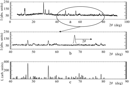
Fig. 1.: General appearance of the experimental diffraction pattern ($a$), a fragment of this diffraction pattern with the test line ($b$), and the corresponding correlation diffraction pattern ($c$)

In Fig. 1, a general schematic diagram of the method is illustrated. Any diffraction pattern is considered as a sample of $n$ elements, where $n$ is the number of scanning angles.  In the diffraction pattern, an interval (window) of $m$ angles is selected, whose width corresponds to the line width, and whose center is in the middle of the selected $m$-interval in the $k$-th angle of a diffraction pattern.  The number of impulses (the intensity) at each angle from this window, $y_{i}$ ($i=1,2,...,k_{0},...,m$), forms a sample for the further analysis.  Then a model sample $z_{i}$ consisting of $m$ elements (angles) is generated in a way to form a bell-shaped line: the $z_{i}$-values are maximum in the middle of the sample and decrease symmetrically toward the edges.  In this work, a Gaussian function, whose shape is close to the shape of a line in the diffraction pattern, was taken for the sake of generation simplicity (see Fig. 1, $b$).  For those two samples, the correlation is calculated using the permutation test.  It is obvious that the correlation will be maximum, if the centers of those lines coincide.  As a result of calculations, a histogram of the possible values for the correlation coefficient is obtained.  The value at the histogram maximum is taken as the value of the correlation coefficient $c_{k}$ and assigned to the $k_{0}$-th element of a new sample of coefficients $c$.  Then the window is shifted to the right by one step, the procedure is repeated, and the element $c_{k+1}$ is calculated.  As a result of the complete scan of the diffraction pattern, a new sample is formed from the elements $c_{k}$ ($k=1,2,...,k_{\max}$), which will be called the correlation diffraction pattern (see Fig. 1, $c$).

The shape of experimental lines is not perfect, especially at low intensities and in the presence of the noise component.  This means that the shape is not reproduced exactly at repeated measurements.  The uncertainty degree for the measured intensity (the area) – under bad conditions, the angle of maximum intensity may also become uncertain – can be estimated using a special statistical analysis, namely, by applying the permutation test [7].

The essence of the latter is as follows.  Let us have a sequence of $n$ angles: $x_{1},x_{2},...,x_{0},...,x_{i},...,x_{n}$.  Then let us define a line as the number of impulses at the $i$-th angle,

$$y_{i}=A_{0}\exp\left[-\frac{{(x_{i}-x_{0})^{2}}}{{2\sigma^{2}}}\right]+\varepsilon_{i},$$ (1)

where $\sigma^{2}$ is the dispersion, $x_{0}$ the position of the curve maximum, and $\varepsilon_{i}$ the random component.  We define the test line as the Gaussian function

$$z_{k}=A_{1}\exp\left[-\frac{{(x_{k}-x_{c})^{2}}}{{2\sigma^{2}}}\right]\!\!,$$ (2)

where $k=1,2,...,m$; $c=m/2$ is the sample middlepoint, and $m\approx\sigma\leq n$.  Now, let us choose $m$ neighbor elements from the sequence $y_{i}$ – i.e. $y_{i},...,y_{i+m}$ – and form the sum

$$S_{j0}=\sum\limits_{k=j}^{m}{y_{k}z_{k}}.$$ (3)

It is easy to verify that this quantity is maximum, when $x_{c}=x_{0}$.  Provided that the set $z_{k}$ is fixed, let us randomly rearrange the elements in the sample $y_{k}$ and calculate a new sum $S_{j}$.  If this procedure is repeated many times, then the percentage $P$ of $S_{j}$-values exceeding $S_{j0}$ will correspond to the probability that the initial sum $S_{j0}$ arose owing to a random relationship between $y_{k}$ and $z_{k}$ (this is the so-called $P$-criterion [7]).  For convenience, the reference point can be shifted to zero, thus introducing the quantity $\Delta S_{j}=S_{j0}-S_{j}$.  Then the negative values of $\Delta S$ testify that a correlation may appear at random $y_{k}$-realizations.  The deviation $L_{j}$ of the maximum in the histogram of the quantities $\Delta S_{j}$ from zero is selected as the correlation magnitude.

One of the key issues of the method developed to find low-intensity lines is the question of how the proposed algorithm treats the background, i.e.  which background is in the correlation diffraction pattern.  To answer it, a diffraction pattern was registered in the absence of the specimen and processed making use of the described correlation method.  In Fig. 2, the result of such a processing of the background signal with no real lines in the diffraction pattern is demonstrated.  Let the notation $\delta$ stand for the background level in the X-ray diffraction data.  Since there are no real lines in the examined signal, a conclusion is drawn that, for the selected processing mode, the background corresponds to the parameter value $\delta\leq 4$.  This means that the discrimination level at the processing of real diffraction patterns has to be not be less than four intensity units in the correlation diffraction pattern.  In other words, all lines in the correlation diffraction pattern with the intensity less than or equal to 4 should be put equal to zero.

7 Verification of the Method
on X-ray Diffraction Data Obtained
for Reference Specimens

The efficiency of the developed correlation analysis method was tested by analyzing the diffraction pattern of the reference $\alpha$-$\mathrm{SiO}_{\mathrm{2}}$ specimen.  Figure 3, $a$ exhibits the corresponding diffraction pattern measured with an angle increment of 0.05^∘.  In Fig. 3, $b$, the same diffraction pattern is shown on a large scale in order to demonstrate the presence of low-intensity lines and the background.  The result of a pattern processing using the correlation method is shown in Fig. 3, $c$.  Here, the correlation diffraction pattern was discriminated at the level $\delta\leq 4$ (see Fig. 2), i.e.  all points in the correlation diffraction pattern that were less than or equal to 4 were put equal to zero.

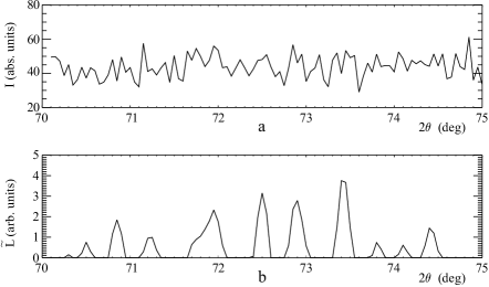
Fig. 2.: Diffraction pattern obtained without a specimen, i.e. the background ($a$); its correlation diffraction pattern ($b$)

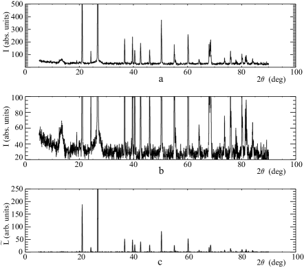
Fig. 3.: General appearance of the diffraction pattern for $\alpha$-quartz ($a$); the same, but scaled up, data ($b$); and the correlation diffraction pattern of $\alpha$-quartz ($c$)

Values of interplanar distances, angles, and normalized intensities for $\bm{\alpha}$-quartz

Our experiment			COD 96-101-1177 [8]			COD 96-153-2513 [9]
$d$, Å	$2\theta$, deg	$\widetilde{\rm I}$	$d$, Å	$2\theta$, deg	$\widetilde{\rm I}$	$d$, Å	$2\theta$, deg	$\widetilde{\rm I}$
1	2	3	4	5	6	7	8	9
4.2205	21.05	186.79	4.2435	20.93	159.35	4.2362	20.97	202.96
3.6703	24.25	18.90
3.3266	26.80	1000	3.3366	26.72	1000	3.3303	26.77	1000
2.4456	36.75	51.92	2.4500	36.68	71.99	2.4457	36.75	75.85
2.2732	39.65	48.25	2.2780	39.56	70.28	2.2734	39.65	76.93
2.2274	40.50	29.69	2.2311	40.43	22.67	2.2271	40.51	34.8
2.1200	42.65	41.15	2.1218	42.62	38.49	2.1181	42.69	52.94
1.9731	46.00	28.55	1.9748	45.96	24.85	1.9713	46.04	30.61
1.8123	50.35	81.89	1.8144	50.29	136.96	1.8109	50.39	116.8
1.7957	50.85	2.01	1.8000	50.72	1.99	1.7962	50.84	3.26
1.6668	55.10	26.74	1.6683	55.05	31.64	1.6651	55.16	40.95
1.6530	55.60	5.23	1.6571	55.45	14.98	1.6537	55.58	16.66
1.6028	57.50	1.38	1.6039	57.46	3.92	1.6011	57.57	2.42
1.5372	60.20	51.85	1.5375	60.19	87.69	1.5348	60.31	87.55
1.4482	64.30	7.41	1.4506	64.21	15.16	1.4477	64.35	17.65
1.4146	66.05	1.78	1.4145	66.05	4.36	1.4121	66.18	3.23
1.3796	67.95	18.03	1.3789	67.98	43.62	1.3764	68.13	53.31
1.3716	68.40	12.55	1.3726	68.34	65.99	1.3699	68.49	61.12
1.3689	68.55	27.78	1.3683	68.58	31.6	1.3659	68.72	42.63
1.2855	73.70	7.42	1.2865	73.63	17.36	1.2838	73.81	22.2
1.2536	75.90	14.66	1.253	75.95	26.75	1.2507	76.11	25.81
1.2405	76.85	1.71
1.2264	77.90	3.51	1.2250	78.00	16.37	1.2229	78.16	12.3
1.1975	80.15	10.46	1.1975	80.15	25.07	1.1952	80.34	28.07
1.1950	80.35	4.11	1.1946	80.38	8.07	1.1926	80.55	8.3
1.1828	81.35	3.60	1.1824	81.39	21.89	1.1800	81.59	21.85
1.1787	81.70	11.00	1.1769	81.85	24.01	1.1749	82.02	26.87
1.1757	81.95	2.36
1.1483	84.35	2.62	1.1499	84.19	18.56	1.1479	84.38	14.06
1.1417	84.95	2.17	1.1390	85.19	2.69	1.1367	85.41	2.61
1.1189	87.10	1.76	1.1156	87.43	0.26	1.1135	87.63	0.22
1.1143	87.55	2.25	1.1122	87.76	2.4	1.1101	87.97	2.55

The values for the angles and the relevant interplanar distances for $\alpha$-quartz from the COD database [5], as well as the values obtained from our experimental data using the correlation method, are quoted in Table.  These results make it possible to draw the following conclusions.

$\bullet$  The values of angles and relative intensities for lines taken from the COD database (see Table, columns 5–6 and 8–9) have the corresponding values in our experimental data (Table, columns 2–3) processed with the help of the described method.

$\bullet$  Close lines at angles of 50^∘, 55^∘, 75.9^∘, 81.5^∘, 84.4^∘, and 87.5^∘ have been resolved and identified, which testifies to a high resolution of the method.

$\bullet$  The method proposed in this work makes it possible to calculate the area and intensity of lines against the “pedestal” background, as is shown in Figs. 3, $a$ and $b$.

8 Capabilities of the Method
for Determining Line Intensities.
A Possibility of Using Classical Methods
for Evaluating the Correlation Coefficient

The analysis made above testifies that the developed correlation method turned out rather sensitive, when searching for an answer to the question: Does a selected angle interval in the diffraction pattern contain a line?  The questions of current concern are as follows: Is it possible to draw quantitative conclusions from the correlation diffraction pattern about the correlation between the areas of the corresponding lines in the initial and correlation diffraction patterns?  Does the correlation diffraction pattern only reflects the degree of correlation between the real and test lines, or it also reflects their intensities?

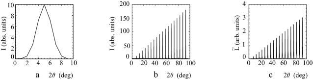
Fig. 4.: Model or test line ($a$), model diffraction pattern formed from model lines with increasing intensities ($b$), and the corresponding correlation diffraction pattern ($c$)

At first glance, the standard Pearson correlation coefficient $q$ given by the expression [10]

$$q=\frac{{\dfrac{1}{n}\sum\limits_{i=1}^{n}{(z_{i}-\bar{z})(y_{i}-\bar{y})}}}{{\sigma_{y}\sigma_{z}}}$$ (4)

seems to be applicable in this case.  When analyzing the model samples (Fig. 4), this coefficient was calculated in parallel with the coefficient $L$ at each permutation, and the value of $q$ at the histogram maximum was taken as the correlation magnitude.  In such a manner, the most probable value of the correlation coefficient was obtained (see, e.g., work [11]).

The both considered methods used in the calculation of the correlation coefficient give information about the correlation degree between two samples.  However, there is a principal difference between the Pearson correlation coefficient and the result of the permutation test.  The Pearson correlation coefficient is introduced by expression (4), and the value of $q$ changes within the interval (0, 1).  At the same time, the correlation value obtained from the permutation test is proportional to expression (3).  Therefore, if the line intensity changes, which is equivalent to the multiplication of a sample $Y$ by a definite coefficient, expression (4) remains unchanged, whereas expression (3) increases by the corresponding factor.

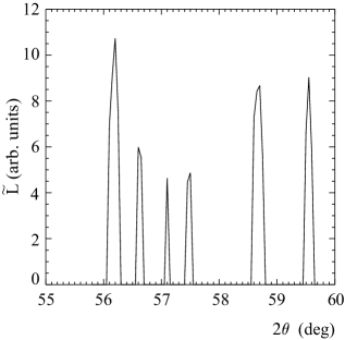
Fig. 5.: Example of a section in the correlation diffraction pattern, which contains additional lines, whose intensities are higher than the intensity of the tabular line at $2\theta=57.46^{\circ}$$\div$$57.57^{\circ}$

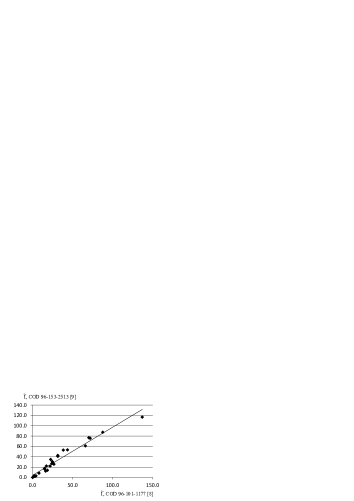
Fig. 6.: Illustration of deviations from the linear relation between the line intensities for $\alpha$-quartz taken from the COD database [5]

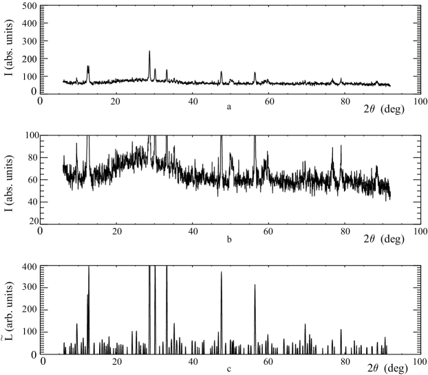
Fig. 7.: General appearance of a brown-ceramic diffraction pattern ($a$); the same, but scaled up, data ($b$); and the correlation diffraction pattern of brown ceramics ($c$)

This statement was verified by means of a direct simulation.  A model diffraction pattern was generated (Fig. 4, $a$), which included a noise background and a series of Gaussian lines with gradually increasing amplitudes (Fig. 4, $b$).  The result of the correlation processing of this signal is shown in Fig. 4, $c$.  One can see that the intensity of correlation lines also increases linearly, which means that there is a linear relationship between the intensities of lines in the original diffraction pattern and the intensities of the corresponding correlation lines.  From whence the following conclusion can be drawn: the amplitude of lines in the correlation diffraction pattern reflects the amplitude of lines in the initial diffraction pattern, but it is obtained in terms of some relative units, because it depends, e.g., on the amplitude of a test line.  Therefore, for the comparison with other data to be possible, the procedure of obtaining the correlation diffraction pattern has to be calibrated.  The required normalizing factor can be obtained, e.g., by analyzing the diffraction pattern for $\alpha$-quartz and equating the amplitude of the maximum correlation diffraction line to 1000, as it is customary to do in databases (see Table).

Figure 4 testifies that there is a linear relationship between the intensities of the experimental and correlation diffraction lines.  Therefore, all lines in the correlation diffraction pattern (after the discrimination of low-intensity lines) are real by definition, including those detected in noise.  Therefore, after the normalization of the correlation diffraction pattern, it can be argued that the relative intensity of experimental diffraction lines (it is determined with a certain error according to the noise level) will be more correct in the correlation diffraction pattern.

This issue can be discussed by analyzing Table, which contains data of various experiments.  One can see that there are some differences between the tabulated data themselves and the data obtained in this work.  The intensities of some lines are very low (the corresponding cells in Table are colored).  At the same time, proceeding from our data, we obtain a paradox.  For instance, the line indicated in the database at $2\theta=57.46^{\circ}$$\div$$57.57^{\circ}$ is also visible in our correlation diffraction pattern (Fig. 5).  However, the same angle interval includes some more low-intensity lines that are not contained in the tabular data, although their intensities are higher than that of the tabular line at $2\theta=57.46^{\circ}$$\div$$57.57^{\circ}$.  This fact means that either several additional lines belonging to $\alpha$-quartz revealed themselves in the correlation spectrum in Fig. 5 or all lines shown in Fig. 5, including the tabular line at $2\theta=57.46^{\circ}$$\div$$57.57^{\circ}$, are “noise”.  The latter may arise as a result of the imperfect character of the reference specimens (both ours and those, the results from which were included into the indicated database).  From whence, it follows that the lines, whose intensities are at the unity level may be real, but not associated with the perfect structure of the crystal lattice in the examined homogeneous material.  A decision of whether they should be taken into account, when identifying the phases by comparing with the tabulated angle values, should have a special substantiation.

On the basis of the data quoted in Table, a plot illustrating the relationship between the tabular values for line intensities taken from the COD database [5] can be drawn (see Fig. 6).  Expectedly, there is a cretain discrepancy between those values, which is a result of the available experimental accuracy of diffraction patterns.  From the results of model calculations (Fig. 4), it follows that there is a linear relationship between the correlation and model intensities (a plot analogous to that in Fig. 6 cannot be drawn for experimental data, because there is no way to independently evaluate the intensities of experimental lines, which are determined exactly in model calculations).  Therefore, it is reasonable to assume that the correlation intensities are more accurate, so that it is better to use the correlation intensities given in column 3 of Table, when estimating the relationships between the $\alpha$-quartz lines.

On the basis of our researches, we may conclude that the method developed for the correlation analysis of diffraction patterns gives reliable results.  This conclusion allowed this method to be applied to the analysis of LLFCMs that look like (and correspondingly dubbed) ’’brown ceramics’’.

In Fig. 7, $a$, the diffraction pattern for a specimen of LLFCM brown ceramics is shown.  The diffraction pattern of this material looks like a noise track with six intense lines and a few broadened ones, e.g., at $\theta\approx 50^{\circ}$ and 60^∘ (see Fig. 7, $b$).  The available data make it possible to reliably identify (on the basis of six lines) and to determine the content of only one phase: uranium oxide UO_2.234 (4.5–5.5 wt.%).  The presence of the following phases are supposed: cubic zirconium oxide $\mathrm{ZrO}_{2}$ (five lines), orthorhombic SiO₂ (one line), and uranium silicate USiO₇ (one line).  For all indicated crystalline phases, their structural (non-chemical) formulas in accordance with the COD database were used.  At first glance, the processing of diffraction data in the framework of our correlation analysis method seems to give a similar picture (Fig. 7, $b$): six intensive lines and a noise track in the form of low-intensity lines.

However, one should bear in mind that “noises” have already been removed from the correlation diffraction pattern.  Therefore, according to the discussion above, all lines in the correlation diffraction pattern should be considered as real.  A comparison of those lines with the X-ray diffraction database [5] brought about an unexpected result.  By analyzing this diffraction pattern, we can not only confirm the identification of uranium oxide UO_2,234, but also reliably identify (on the basis of more than six lines) and determine the content of cubic zirconium oxide ZrO₂ (2–3 wt.%), orthorhombic silicon oxide SiO₂ (3–5 wt.%), and uranium silicate USiO₇ (3–4 wt.%).  The correlation diffraction pattern allowed the identification of phases with the content not only at a level of 1 wt.% ($\mathrm{Al}_{0.32}\mathrm{Si}_{0.68}\mathrm{O}_{2}$), but also lower than 1 wt.%, namely, triclinic silicon oxide (0.4–0.5$\mathrm{\leavevmode\nobreak\ wt.\%}$), cubic silicon oxide SiO₂ (0.2–0.4$\mathrm{\leavevmode\nobreak\ wt.\%}$), calcium silicate CaSiO₃ (0.15–0.3 wt.%), and calcium silicate $\mathrm{Ca}_{3}\mathrm{Si}_{2}\mathrm{O}_{6}$ (0.1–0.2$\mathrm{\leavevmode\nobreak\ wt.\%}$).

We note that the high sensitivity and accuracy of the method poses a new problem. The existence of a great number of low-intense lines at the analysis ‘‘by hands’’ increases the error of determination of their relative contribution (errors can increase by several times). The question about the development of a method of reliable evaluation of the content of phases in such situation will be considered in the subsequent works.

From the viewpoint of the X-ray diffractometry practice, this result of the crystalline phase identification by processing the diffraction patterns can be regarded as a very good one.

9 Conclusions

A method to detect low-intensity X-ray lines has been developed for the problems of X-ray phase analysis of materials that contain many (more than eight) low-content (from several tenths of wt.% to a few wt.%) crystalline phases.  The method is based on the calculation of correlations with the use of the computer statistics approaches.

The application of this method to reference specimens showed not only its efficiency, but also its advantages, when determining the line intensities.  In particular, in many cases, when the database contains only a qualitative indication that the intensity of corresponding lines is actually lower than the identification level, the developed method allowed the corresponding intensity value to be assigned to each detected line (see Table).

The application of the developed correlation method to the analysis of the diffraction patterns of specimens containing phases with a content lower than 0.1 wt.% showed that such phases can be reliably identified.  The determination of the lower sensitivity limit of the method is a task for the further research.

The work was sponsored in the framework of the budget theme of the National Academy of Sciences of Ukraine (No. 0117U002636).

А.Д. Скорбун, С.В. Габєлков, I.В. Жиганюк,
В.Г. Кудлай, П.Є. Пархомчук, С.О. Чиколовець
МЕТОД ОБРОБКИ ДАНИХ РЕНТГЕНIВСЬКОЇ
ДИФРАКЦIЇ ДЛЯ БАГАТОФАЗНИХ МАТЕРIАЛIВ
З НИЗЬКИМ ВМIСТОМ ФАЗ
Р е з ю м е
Пiд час дослiдження методом рентгенiвського фазового аналiзу аморфних, скляних та склокерамiчних матерiалiв, якi практично завжди мають у своєму складi значну кiлькiсть кристалiчних фаз (бiльше восьми) з їх вмiстом вiд декiлькох % мас. до декiлькох десятих – сотих % мас., виникають труднощi з визначенням фазового складу. Розроблено метод аналiзу дифрактограм таких матерiалiв, коли на дифрактограмах спостерiгаються рентгенiвськi лiнiї, iнтенсивнiсть яких знаходиться на рiвнi шумiв. Виявлення лiнiй базується на використаннi пошуку кореляцiй мiж експериментальною i тестовою лiнiями i перевiрцi збiгiв за допомогою статистичних методiв аналiзу (комп’ютерна статистика). Метод перевiрено на зразках $\alpha$-кварцу, який часто використовується як еталон, та застосовано до аналiзу лавоподiбних паливовмiсних матерiалiв Чорнобильської АЕС. Показано, що розроблена методика дозволяє iдентифiкувати рентгенiвськi лiнiї при вмiстi окремих фаз до $0{,}1$ % мас., а також iстотно пiдвищує можливiсть кiлькiсно визначати вмiст фази за лiнiями з слабкою iнтенсивнiстю.

References

- [1] R.V. Arutyunyan, L.A. Bolshov, A.A. Borovoi, E.P. Velikhov, A.A. Klyuchnikov. Nuclear Fuel in the “Shelter” Facility of the Chernobyl NPP (Nauka, 2010) (in Russian).
- [2] S.V. Gabielkov, A.V. Nosovskii, V.N. Shcherbin. Degradation model of lava-like fuel-containing materials in the “Shelter” facility. Probl. Bezpek. At. Elektrost. Chornobyl. 26, 75 (2016) (in Russian).
- [3] S.V. Gabielkov, I.V. Zhyganiuk, V.G. Kudlai, P.E. Parkhomchuk, S.A. Chikolovets. Crystallization of lava-like fuel-containing materials NBK-OU. Probl. Bezpek. At. Elektrost. Chornobyl. 32, 44 (2019) (in Ukrainian).
- [4] Phase Identification from Powder Diffraction ‘‘Match!’’. Version 3.7.1.132, Crystal Impact, Bonn, Germany [http://www.crystalimpact.com].
- [5] S. Gražsulis, A. Merkys, A. Vaitkus, M. Okulič-Kazarinas. Computing stoichiometric molecular composition from crystal structures. J. Appl. Crystallogr. 48, 85 (2015).
- [6] A.D. Scorbun, M.I. Panasyuk. Resolution of low-intensity lines in gamma spectra. Probl. Bezpek. At. Elektrost. Chornobyl. 9, 125 (2008) (in Ukrainian).
- [7] D.S. Moore, G.P. McCabe, B.A. Craig. Introduction to the Practice of Statistics (Freeman, 2014) [ISBN: 1464158932].
- [8] F. Machatschki. Die kristallstruktur von tiefquarz und aluminiumorthoarsenat . Z. Kristallogr. Krist. 94, 222 (1936).
- [9] P. Kroll, M. Milko. Theoretical investigation of the solid state reaction of silicon nitride and silicon dioxide forming silicon oxynitride () under pressure. Z. Anorg. Allg. Chem. 629, 1737 (2003).
- [10] D.J. Hudson. Statistics. Lectures on Elementary Statistics and Probability (CERN, 1964).
-
[11]
H. Tanizaki. On small sample properties of permutation
tests: Independence test between two samples. Int. J. Pure
Appl. Math. 13, 235 (2004) [ISSN: 1311-8080].
Received 07.05.19.
Translated from Ukrainian by O.I. Voitenko