Violation of Stokes-Einstein and Stokes-Einstein-Debye relations in polymers at the gas-supercooled liquid coexistence

Abstract

Molecular dynamics simulations are performed on a system of model linear polymers to look at the violations of Stokes-Einstein (SE) and Stokes-Einstein-Debye (SED) relations near the mode coupling theory transition temperature $T_{c}$ at three (one higher and two lower) densities. At low temperatures, both lower density systems show stable gas-supercooled-liquid coexistence whereas the higher density system is homogeneous. We show that monomer density relaxation exhibits SE violation for all three densities, whereas molecular density relaxation shows a weak violation of the SE relation near $T_{c}$ in both lower density systems. This study identifies disparity in monomer mobility and observation of jumplike motion in the typical monomer trajectories resulting in the SE violations. In addition to the SE violation, a weak SED violation is observed in the gas-supercooled-liquid coexisting domains of the lower densities. Both lower density systems also show a decoupling of translational and rotational dynamics in this polymer system.

I Introduction

Simple liquids show coupling of translational diffusion coefficient $D$ and viscosity $\eta$ through the SE relation Hansen and McDonald (2006); Stokes (1851); Einstein (1905)

$$D=\frac{k_{B}T}{c\pi\eta r},$$ (1)

where $k_{B}$ is the Boltzmann constant, $r$ is effective hydrodynamic radius of a Brownian particle immersed in the fluid. The constants $c=$ 4 and 6 in Eq. (1) are respectively for slip and stick boundary conditions. Thus, Eq. (1) can be written as $D\eta/T=$ constant that is obeyed in the liquids at high temperatures. A calculation of $\eta$ of a system is computationally expensive in the supercooled liquids due to the large fluctuations in their stress autocorrelation functions Kawasaki and Kim (2017). Therefore, instead of viscosity $\eta$, the relaxation time $\tau$ is computed from the simulations of glass-forming liquids (GFLs) with the approximation $\tau\propto\eta/T$ Sengupta et al. (2013); Bhowmik et al. (2016); Shi et al. (2013); Yamamoto and Onuki (1998); sen . Deviations from $D\tau=$ constant are considered as the SE violations due to the decoupling in $D$ and $\tau$. These violations of the SE relation have been observed in simulations Sengupta et al. (2013); Becker et al. (2006); Puosi and Leporini (2012); Pan et al. (2017) and experiments Ediger (2000); Andreozzi et al. (1996); Edmond et al. (2012); Mishra and Ganapathy (2015) of several supercooled GFLs. Earlier studies show that a possible reason for the violation of the SE relation is dynamical heterogeneity (DH) in the supercooled liquids Ediger (2000); Berthier et al. (2011); Flenner et al. (2014). There is a consensus among the glass community that glassy systems lose homogeneity in the dynamics due to the presence of mobile (fast-moving) and immobile (caged) particles Donati et al. (1999), noticeably in fragile GFLs Ediger (2000). The mobile particles move faster than the average motion, while immobile particles move slowly in the system, leading to the DH Ediger (2000); Glotzer (2000); Richert (2002); Donati et al. (1999); Kob et al. (1997); Berthier et al. (2011); Flenner et al. (2014).

Near the glass transition, $D$ is dominated by the mobile particles, whereas $\tau$ is governed by the immobile particles (as the majority of the particles are caged). Increment in $\tau$ is not accompanied by the decrement in $D$ due to different mobilities in the system, causing a decoupling in $D$ and $\tau$, which results in the breakdown of the SE relation. It has been argued that the hopping of particles from the cages formed by their neighbors has a role in the violation of the SE relation in the supercooled GFLs Charbonneau et al. (2014); Chong (2008); Zou et al. (2019). A study on supercooled hard-sphere liquid by Kumar et al. Kumar et al. (2006) shows that the SE relation violates due to the presence of mobile particles, whereas immobile particles obey it. However, few recent studies show that both mobile and immobile particles violate the SE relation Becker et al. (2006); Pan et al. (2017).

In molecular GFLs, system shows violation of SED relation connecting orientational relaxation and viscosity of the liquid. The relaxation time of rotational correlation function $\tau_{l}$, defined using $l$th order Legendre polynomial, is related to the viscosity $\eta$ via SED relation Debye (1929); Berne and Pecora (2000); Tarjus and Kivelson (1995)

$$\frac{1}{\tau_{l}}=\frac{l(l+1)k_{B}T}{6\eta V_{h}},$$ (2)

where $V_{h}=(4/3)\pi R_{h}^{3}$ is the hydrodynamic volume of a molecule; $R_{h}$ is the effective hydrodynamic radius of the molecules. Hydrodynamic radius $R_{h}$ and radius of gyration $R_{g}$ are unequal, in general. However, they are related in the Kirkwood approximation Doi and Edwards (1986); de Gennes (1979); Kirkwood (1954). Few recent studies, on the relation between $R_{g}$ and $R_{h}$ of the longer polymer chains, show that $R_{g}/R_{h}=a$ Rubinstein and Colby (2003); Mansfield et al. (2015); Clisby and Dünweg (2016); Vargas-Lara et al. (2017). Here $a$ is a constant depending on the molecular weight, topology, etc. of the polymers. In addition to this, Costigliola et al. Costigliola et al. (2019) and Ohtori et al. Ohtori and Ishii (2015); Ohtori et al. (2018) revisit the Stokes-Einstein relation showing that $R_{h}\propto\rho^{{-1}/3}$, which modifies the relation as

$$\frac{D\eta}{\rho^{1/3}k_{B}T}=\textnormal{const}.$$ (3)

This relation omits the importance of hydrodynamic diameter and rely instead on the system density $\rho$; these authors examined the relation in Lennard-Jones liquids above the critical density. The coupling between viscosity $\eta$ and rotational correlation time $\tau_{l}$ of molecular liquids holds the SED relation at high temperatures, whereas it violates in the supercooled liquids and glasses Mazza et al. (2007); Andreozzi et al. (1996); Ngai (1999). Using this approximation, Eq. (2), and Eq. (1) suggest that $D\tau_{l}=$ constant in molecular liquids at high temperatures Tarjus and Kivelson (1995). Thus, the translational molecular diffusion $D$ is coupled to the rotational relaxation time $\tau_{l}$ of the molecules. However, simulation studies by Michele et al. Michele and Leporini (2001a, b) show translational and rotational jump dynamics leads to violation of SE and SED relations in a system of diatomic rigid-dumbbell molecules.

Extending such studies (performed on binary mixtures and dumbbells) to polymers is a daunting task due to the complexity of the system. Identification of jumplike motions are reported in the continuous-time random walk simulation of Helfferich et al. Helfferich et al. (2014) with a special definition of the jumps in a supercooled short-chain melt. Another study by Pousi et al. Puosi and Leporini (2012); Puosi et al. (2018) argued that picosecond dynamics of the caged particles corresponding to short time ($\beta-$relaxation), is related to the violation of SE relation in supercooled linear polymers. A very recent study shows that the violation of SE relation is related to the structural changes in the supercooled linear polymer melt Balbuena and Soul$\acute{e}$ (2020). Therefore, due to the molecular complexity, it is strenuous to examine the SE and SED violation in polymer liquids and to identify a possible reason compared to the simulation studies of atomic GFLs. This study attempts a direct identification of SE and SED violations in a simple polymer model that is known to undergo glass transition and relates it to the known reasons that are manifestations of DH in atomic GFLs.

Polymers are extended molecules that relax by collective rearrangements of monomers. Therefore, identification of the mobile and immobile particles is expected to be easier in low density where there is more free-space available at lower temperatures. Polymer systems with attractive interactions in the lower density show coexistence of dilute gas and supercooled liquid domains at lower temperatures with cavities. On the surface of these cavities, there is free space available for chains leading to a large variation in mobilities, which can show direct evidence of SE and SED violations and their possible microscopic origins. In this study, we examine the violations of the SE and SED relations in a linear polymer system at number densities $\rho=$ 1.0 Starr et al. (2002), 0.85 Bennemann et al. (1998), and 0.7, which we call as one higher and two lower (relatively) density systems, from $T=$ 2.0 to near their respective $T_{c}$ (in unequal grids of temperature), i.e., 0.36 for the higher density and 0.4 for both lower densities. Both lower density systems are quenched to temperatures beyond the spinodal limit of stability, which phase separate via spinodal decomposition Huang (2010) resulting in stable coexistence of (dilute) gas and supercooled-liquid with long equilibration times. Details of non-equilibrium dynamics of cavity formation are given in earlier studies Foffi et al. (2005); Cardinaux et al. (2007); Godfrin et al. (2018); Chaudhuri and Horbach (2016); Testard et al. (2011). Recently, Priezjev and Makeev examined an effect of shear strain on the porous structure in a model binary glass in non-equilibrium Priezjev and Makeev (2017); Makeev and Priezjev (2018). In our study, monomer relaxation shows SE violation in all three systems; both lower density systems show pronounced violation that is attributed to the enhanced disparity in the motion of the monomers that arises due to the surface of the cavities. A pronounced violation of SE relation is due to both the mobile and immobile particles, which agrees with the earlier studies on violation of SE and SED relations in atomic model GFLs Becker et al. (2006); Pan et al. (2017). The SED relation is obeyed in the higher density system, whereas it is weakly violated in both lower density systems.

The rest of the manuscript is organized as follows: Sec. II gives the details of the simulations. Results are presented in subsections of III. Subsec. III.1 present stability analysis of the phase coexistence of gas-supercooled-liquid. The study of polymer relaxation and diffusion is presented in Subsec. III.2, SE violations are discussed in Subsec. III.3, the distribution of particles’ mobility and jumplike motions are presented in Subsec. III.4, and violation of SED relation and orientational relaxation are detailed in Subsec. III.5. Finally, Sec. IV presents conclusions and a short summary.

II Simulation details

We simulate a system of $N_{c}=$ 1000 fully-flexible linear polymer chains, consisting of $n=$ 10 beads in each. Thus, the system consisting of $N=$ 10000 number of monomers is simulated at constant number density of monomers, i.e., $\rho=$ 0.7, 0.85, and 1.0. Inter-particle interactions are modeled by truncated and shifted Lennard-Jones (LJ) potential, defined in terms of the particle diameter, $\sigma$ and the depth of the potential well, $\epsilon$ as

$$V_{LJ}(r)=4\epsilon\left[\left(\frac{\sigma}{r}\right)^{12}-\left(\frac{\sigma}{r}\right)^{6}\right]-V_{LJ}(r_{c}).$$ (4)

Here, the LJ potential cut-off is $r_{c}=2\times 2^{1/6}\sigma$. The bond connectivity between consecutive monomers along a chain is modeled by the LJ and finitely extensible non-linear elastic (FENE) potentials Grest and Kremer (1986); Bennemann et al. (1998); the FENE potential is given in terms of $R_{0}$, the maximum displacement between a pair of consecutive monomers, and the elastic constant $k_{0}$ as

$$V_{FENE}(r)=\begin{cases}-\frac{1}{2}k_{0}R^{2}_{0}\ln\left(1-\frac{r^{2}}{R^{2}_{0}}\right)-E_{b}&0<r<R_{0}\\ \infty&r\geq R_{0},\end{cases}$$ (5)

where $k_{0}=30\epsilon/\sigma^{2}$ and $R_{0}=1.5\sigma$. The equations of motion are integrated using the velocity Verlet algorithm Allen and Tildesley (1987) with time step $\Delta t=$ 0.002 for $\rho=$ 0.85, and $\Delta t=$ 0.0001 for $\rho=$ 1.0 and 0.7 system. We prepare the linear polymer melt at temperature $T=$ 8.0, for the respective density, in the microcanonical (constant NVE) ensemble. The equilibrated configurations at $T=$ 8.0 are used as the initial configurations for the temperatures $T=$ 2.0–0.36. Long simulation time before the production runs ensures fluctuation of the system around the average target temperature during the data collection in constant NVE ensemble and follow a criterion of the time required for the relaxation of end-to-end vector below $10\%$ of its initial value at all temperatures Helfferich et al. (2014). All the quantities presented in this work are in LJ units, i.e., the length is expressed in terms of the bead diameter $\sigma$, the number density as $\sigma^{-3}$, the temperature as $\epsilon/k_{B}$, and the time as $\sqrt{m\sigma^{2}/\epsilon}$.

III Results and discussions

III.1 Steady-state density relaxation in gas-supercooled-liquid domains

State points corresponding to decreasing order of temperatures in both lower density systems show coexistence of gas and liquid at intermediate temperatures, e.g., $T=0.7$ for $\rho=$ 0.85, and $T=$ 1.0 for $\rho=$ 0.7 (see Fig. 8 and Fig. A.2). However, the system shows the phase-coexistence of dilute gas and supercooled liquid at lower temperatures. In the moderately supercooled state, the system attains its steady-state where the cavities are stable, whereas the cavities at the liquid-gas phase coexistence move, thus the system attains density relaxation. Before presenting the glass transition studies, we look at the single-particle and collective density relaxation to ensure the ergodicity of the system. Studies on aging compare the time-origin dependent density-relaxation using incoherent intermediate scattering function $F_{s}(k,t)$ Kob and Barrat (1997), which show different relaxation time for different time origins. Therefore, we look into the relaxation of density fluctuations in $F_{s}(k,t)$ Hansen and McDonald (2006) at time origins longer than the $\alpha-$relaxation time (presented later in this paper), which is defined as

$$F_{s}(k,t)=\frac{1}{N}\left\langle\rho^{s}_{\mathbf{k}}(t)\rho^{s}_{-\mathbf{k}}(0)\right\rangle,$$ (6)

where $\rho^{s}_{\mathbf{k}}(t)=\exp[-i\mathbf{k}\cdot\mathbf{r}_{i}(t)]$. Here, $k$ is the wavenumber and $\mathbf{r}_{i}$ is the position vector of an $i^{th}$ particle. The $F_{s}(k,t)$ shown in Fig. 1 is calculated at a wavenumber $k$ that corresponds to the first peak of static structure factor $S(k)$; $k=$ 6.9 for $\rho=$ 0.85 and $k=$ 7.1 for $\rho=$ 0.7 and $\rho=$ 1.0. The $\alpha-$relaxation time of the monomers $\tau_{\alpha}=\int_{0}^{\infty}F_{s}(k,t)dt$ gives the relaxation time of transient cages formed by their neighbouring particles. The time difference between two time origins is chosen to be greater than $\tau_{\alpha}$ (see Fig. A.3 for $\tau_{\alpha}$) to look at the average density relaxation of monomers in that time window. The $F_{s}(k,t)$ of all three densities at the lowest temperatures, given in Figs. 1(a–c), does not show any systematic variation in the nature of density relaxation with time, at different time origins of the correlation, therefore, they are independent of the time origin. A small difference due to fluctuations in the tail of $F_{s}(k,t)$ in lower densities is similar to that at the higher density.

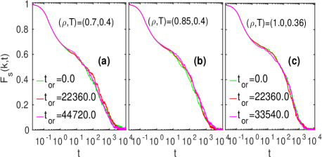
Figure 1: Incoherent intermediate scattering function, $F_{s}(k,t)$ of monomers is calculated at different time origins of the low temperatures. The legend in (b) is same as in (c).

Collective relaxation dynamics of the phase-coexisting system is examined by distinct part of van-Hove correlation function, $G_{d}(r,t)$ Hansen and McDonald (2006),

$$G_{d}(\mathbf{r},t)=\frac{1}{N}\left\langle{\sum\limits_{i=1}^{N}\sum\limits_{j=i+1}^{N}{\delta[\mathbf{{r}}+{\mathbf{r}}_{i}(0)-{\mathbf{r}}_{j}(t)]}}\right\rangle,$$ (7)

that shows collective structural relaxation in different coordination shells with respect to a reference particle at $t=0$. Figure 2 shows the $G_{d}(r,t)/\rho$ of the monomers at one low and one high temperature of both lower densities at different times starting from $t=0$. At $t=$ 0, $G_{d}(r,0)/\rho=g(r)$ is showing oscillations with mean above 1.0, which is due to the phase separation in the system. The neighboring particles around a tagged particle move from their initial positions (as time progresses), leading to decay of the $G_{d}(r,t)$ to 1.0 as in a homogeneous system ($T=$ 1.0). However, $G_{d}(r,t)/\rho$ remains above 1.0 for both lower density systems that show coexistence of dilute gas and supercooled liquid domains at low temperatures even at longest time scale in this study. Interestingly, Fig. 2 shows that the $G_{d}(r,t)$ of both lower densities coincides at times $t=5\times 10^{3}$ and $t=1.5\times 10^{5}$, which shows that the shape and location of the cavities are stable and do not change within our simulation time in the moderately supercooled state. It is now interesting to look at polymer relaxation dynamics in the higher and both lower density systems as temperature reduces.

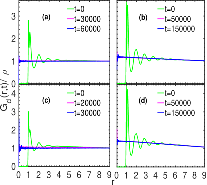
Figure 2: Distinct part of van-Hove correlation function scaled with the density is plotted in (a) $\rho=$ 0.85, $T=$ 0.7; (b) $\rho=$ 0.85, $T=$ 0.4; (c) $\rho=$ 0.7, $T=$ 1.0; (d) $\rho=$ 0.7, $T=$ 0.4.

III.2 Polymer relaxation and diffusion

The self-diffusion coefficient $D$ of the monomers is calculated from their mean-squared displacement (MSD) as $D=\lim\limits_{t\to\infty}{\langle[{\mathbf{r}}(t)-\mathbf{r}(0)]^{2}\rangle}/{6t}$. Near the glass transition of unentangled polymer melts, the monomer MSD takes longer time to attain diffusive regime due to the chain connectivity Barrat et al. (2010). Therefore, the monomer MSD shows a power law dependency as ${\langle[{\mathbf{r}}(t)-\mathbf{r}(0)]^{2}\rangle}\sim t^{0.63}$, before the starting of its diffusion Barrat et al. (2010). However, the MSD of the polymer molecules (center of mass) shows the diffusion at early times, though they are slow at short time and coincides with the monomer MSD at the long times $t\simeq 10^{6}$ Barrat et al. (2010); Chong and Fuchs (2002). Therefore, we calculate the self diffusion coefficient from the center of mass MSD — when the exponent $\alpha=$ 1.0 in the relation $g_{2}(t)=\langle[\mathbf{r}_{cm}(t)-\mathbf{r}_{cm}(0)]^{2}\rangle=6Dt^{\alpha}$, where $t>10^{5}$ in the LJ units at the lowest temperatures (see Fig. 3). At this time scale, the molecular MSD also crosses the average squared end-to-end distance, i.e., $g_{2}(t)>R^{2}_{e}$, which is indicated by the red line at $g_{2}(t)=R^{2}_{e}$ in Fig. 3. Using the approximation $\tau\propto\eta/T$ (as discussed above), the fractional SE relation reads $D\sim\tau^{-\xi}$ ($0<\xi<1$), which shows that the diffusion coefficient and relaxation time (or viscosity) decouple from the usual SE relation, i.e., Eq. 1, which is also reported in various earlier studies of supercooled liquids and glasses Kumar et al. (2006); Flenner et al. (2014); Becker et al. (2006); Mishra and Ganapathy (2015).

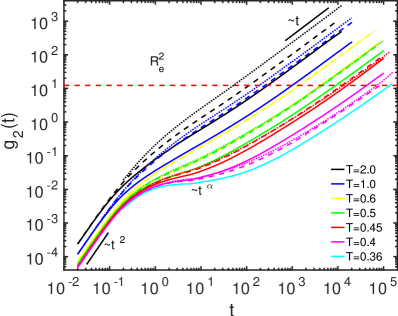
Figure 3: Center of mass MSD of chains, $g_{2}(t)$ is plotted against time $t$. Solid, dashed, and dotted lines are corresponding to the density $\rho=$ 1.0, 0.85, and 0.7 respectively. At temperatures $T=$ 2.0–0.45, $g_{2}(t)$ of the higher density system is slower than both lower density systems. However, both lower density systems show slow molecular movement than the higher density system from $T=$ 0.4 to below. At low temperatures ($T=$ 0.5–0.4), the sub-diffusive regime ($g_{2}(t)\sim t^{\alpha}$) becomes pronounced due to the molecular cages, which is separated by the short time ballistic ($g_{2}(t)\sim t^{2}$) and long time diffusive ($g_{2}(t)\sim t$) regimes.

Earlier studies argued that one of the possible reason for the violation of SE relation is the caging and hoping of the particles in supercooled liquids, which results in the spatially heterogeneous dynamics Ediger (2000); Berthier et al. (2011); Flenner et al. (2014); Charbonneau et al. (2014); Chong (2008); Zou et al. (2019). The slow down of density relaxation due to transient caging, and an increase in the relaxation time with a reduction in the temperature, can be examined from the $F_{s}(k,t)$. Figure 4(a) shows $F_{s}(k,t)$ of monomers at the wavenumber $k=$ 6.9 for $\rho=$ 0.85, and $k=$ 7.1 for $\rho=$ 0.7 and $\rho=$ 1.0, at all the temperatures. As temperature reduces, a hump appears in $F_{s}(k,t)$ from temperature $T=$ 0.5 for both lower densities, whereas it starts from $T=$ 0.6 for the higher density system. The appearance of a hump in the $F_{s}(k,t)$ of all three systems indicates a commencement of monomer caging that enhances their $\alpha$-relaxation time. It is evident from Fig. 4(a) that $F_{s}(k,t)$ of both lower density systems shows slower relaxation dynamics than that of the higher density system at $T=$ 0.4, thus show a crossover. The heterogeneity in the relaxation is quantified from fitting the tail of $F_{s}(k,t)$ with empirical Kohlrausch-Williams-Watts (KWW) function $f(t)^{KWW}\!\propto\ \exp[-(t/\tau)^{\beta}]$ below temperature $T=$ 2.0 with the value of exponent $\beta$ varies from 0.92 to 0.59 for $\rho=$ 0.85, 0.94 to 0.55 for $\rho=$ 0.7, and from 0.85 to 0.72 for the higher density system. This shows that lower densities exhibit more heterogeneous dynamics, which is a result of heterogeneous density distribution due to the formation of the cavities (see nearest neighbour distribution in Fig. A.2). We fit $\tau_{\alpha}$ vs $T$ curves (see Fig. A.3) using schematic mode coupling theory (MCT) and Vogel-Fulcher-Tammann (VFT) relations, respectively, as $\tau_{\alpha}\!\propto(T-T_{c})^{-\gamma}$ and $\tau_{\alpha}\!\propto\exp(AT_{0}/(T-T_{0}))$. The fitting parameters of these two equations for the density $\rho=$ 1.0, 0.85, and 0.7 are shown in Table 1. The fragility parameter $A$ obtained from the VFT fit shows that lower density systems are more fragile than the higher density system.

Table 1: Fitting parameters for the MCT and VFT relations at three densities: MCT transition temperature $T_{c}$, MCT exponent $\gamma$, dynamic divergence temperature $T_{0}$, and fragility parameter $A$. $T_{c}$ and $T_{0}$ are lower for the higher density system and fragility is smaller as fragility $\propto$ $1/A$ Angel (1995).

Density	MCT fitting		VFT fitting
	$T_{c}$	$\gamma$	$T_{0}$	$A$
$\rho=$ 1.0	0.33	1.79	0.19	6.6
$\rho=$ 0.85	0.39	1.71	0.31	2.12
$\rho=$ 0.7	0.39	1.87	0.3	2.69

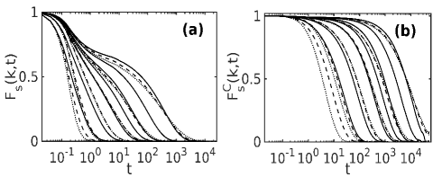
Figure 4: Incoherent intermediate scattering function of monomers (a) and Center of mass (b). Solid, dashed, and dotted lines correspond to the densities $\rho=$ 1.0, $\rho=$ 0.85, and $\rho=$ 0.7. In (a) and (b) temperature decreases from left to right as $T=$ 2.0, 1.0, 0.6, 0.5, 0.45, 0.4, 0.36 ($\rho=$ 1.0 only).

The molecular density relaxation is studied from the time variation of molecular self-intermediate scattering function

$$F^{C}_{s}(k,t)=N_{c}^{-1}\left\langle\rho^{C}_{\mathbf{k}}(t)\rho^{C}_{-\mathbf{k}}(0)\right\rangle,$$ (8)

where $\rho^{C}_{\mathbf{k}}(t)=\exp[-i\mathbf{k}\cdot\mathbf{r}^{cm}(t)]$ and $\mathbf{r}^{cm}(t)$ is the position of the center of mass of a polymer molecule at time $t$. Figure 4(b) shows that the $F^{C}_{s}(k,t)$ of lower and higher density systems are plotted against time $t$ at $T=$ 2.0-0.36, and the wavenumber $k=2\pi/2R_{g}\sim$ 2.1. Here, $R_{g}$ is the average radius of gyration of polymer chains in both lower and the higher density systems, and its values are 1.46 and 1.45. Thus, molecular diameters are $2R_{g}=$ 2.92 and 2.9, and we consider $2R_{g}=$ 2.9. In Fig. 4(b), the $F^{C}_{s}(k,t)$ of both lower density systems shows crossover to the longer relaxation time in comparison to the higher density system at the same temperature $T=$ 0.4; the $F^{C}_{s}(k,t)$ of both lower density systems at $T=$ 0.4 is comparable to the $F^{C}_{s}(k,t)$ of the higher density system at $T=$ 0.36. To examine the time scale of the molecular relaxations, we calculate molecular relaxation time $\tau_{2R_{g}}=\int_{0}^{\infty}F^{C}_{s}(k,t)dt$, which is higher at high (and intermediate) temperatures for the higher density system compare to both lower density systems. However, in the moderately supercooled regime (near $T_{c}$) there is a crossover similar to the case of monomer density relaxation (see Fig. A.6). Now, we look into the violation of SE and SED relations at these state points of the system.

III.3 Violation of Stokes-Einstein relations

To look at the violation of SE relation, we compute exponent of the power-law dependence of diffusion constant on the relaxation time, i.e., $D\sim\tau^{-\xi}_{\alpha}$ at different densities. Figure 5 shows that $\xi=$ 1.0 for the higher density, whereas $\xi=$ 1.38 and 1.3 for $\rho=$ 0.7 and 0.85, respectively, in the temperature range $T=$ 2.0–0.6. Exponent $\xi>1$ shows the decoupling of $D$ and $\tau_{\alpha}$ in the normal liquid temperatures, which is also reported in many studies including Refs. Sengupta et al. (2013); Li et al. (2019). In moderately supercooled regime ($T=$ 0.5–0.36), the value of $\xi=$ 0.83 for the higher density system, and $\xi=$ 0.73 and 0.66 for $\rho=$ 0.85 and 0.7, respectively, thus shows decoupling of $D$ and $\tau_{\alpha}$. The decreasing value of $\xi$ with the density suggests that the decoupling increases with decreasing density. A smaller value of $\xi$ in the supercooled regime of both lower density systems shows the pronounced violation of the SE relation, and in particular, the violation is more pronounced for the lower density $\rho=$ 0.7. In both lower density systems, effective attraction between particles is pronounced, in contrast to the higher density system. A study on attractive and repulsive colloidal glasses also shows the stronger violation of the Stokes-Einstein relation in the attractive glassy colloids Puertas et al. (2007) .

Another way of estimating the SE breakdown is the predictors of violation of the SE relation Sengupta et al. (2013); Bhowmik et al. (2016); Shi et al. (2013); Yamamoto and Onuki (1998), e.g., $D\tau_{\alpha}(T)$. We compute SE ratio as $D\tau_{\alpha}(T)/D\tau_{\alpha}(T=1.0)$, where $D\tau_{\alpha}$ at temperature $T=$ 1.0 is a reference point, as given in Fig. 6(a). Figure 6(a) shows that the SE ratio starts decreasing below $T=$ 1.0, which again starts increasing from $T=$ 0.5 and reaches values around 2.1 and 2.7, respectively, at the lowest temperature $T=$ 0.4 of the density $\rho=$ 0.85 and $\rho=$ 0.7. In the higher density system, the SE ratio remains constant up to $T=$ 0.6, which starts increasing from $T=$ 0.5 and attains a value around 2.0 at the lowest temperature $T=$ 0.36. Below temperature $T=$ 0.5, where fractional SE relation is found at all three densities (see Fig . 5), the SE ratio also starts increasing. A higher value of the SE ratio correlates with the smaller value of the fractional SE exponent $\xi$. Thus, we show that the SE relation breaks down in the supercooled linear polymers for all three densities.

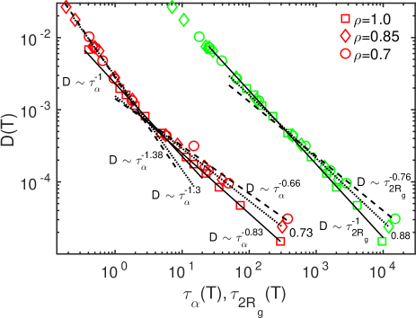
Figure 5: Self diffusion coefficient $D(T)$ is plotted against $\tau_{\alpha}(T)$ (red) and $\tau_{2R_{g}}(T)$ (green). Solid, dotted, and dashed lines are fit to the data at densities $\rho=$ 1.0, 0.85, and 0.7, respectively: the data is fitted using relations $D\sim\tau^{-\xi}_{\alpha}$ and $D\sim\tau^{-\xi}_{2R_{g}}$ for monomers and molecules, respectively.

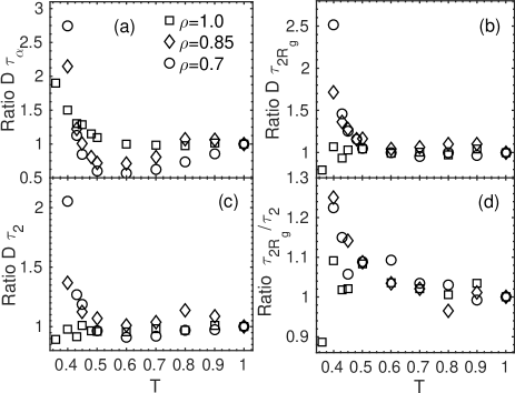
Figure 6: Ratios of (a) $D\tau_{\alpha}$, (b) $D{\tau_{2R_{g}}}$, (c) $D\tau_{2}$, and (d) $\tau_{2R_{g}}/\tau_{2}$ are plotted against temperature $T$. The ratios are defined as $D\tau(T)/D\tau(T=1.0)$, where $D\tau(T=1.0)$ is a reference point.

Polymer chains in this study are flexible, which shows large shape fluctuations. Therefore, it is compelling to examine the violations of the SE relation at the molecular level. Diffusion constant $D$ is plotted against molecular relaxation in Fig. 5, where data is fitted using the relation $D\sim\tau^{-\xi}_{2R_{g}}$. A variation in $\tau_{2R_{g}}$ with temperature is shown in Fig. A.6. The value of the exponent $\xi$ is 1.0 from $T=$ 2.0–0.6 for both lower density systems. However, in the supercooled regime ($T=$ 0.5–0.4), the value of the exponent $\xi$ are 0.88 and 0.76, respectively for the density $\rho=$ 0.85 and $\rho=$ 0.7, thus, show a weak (exponent $\xi$ closer to unity) violation of molecular SE relation; the extent of violation is more at $\rho=$ 0.7. On the other hand, $\xi=$ 1.0 for whole temperature range (of this study) at the higher density, thus, $D$ and $\tau_{2R_{g}}$ are coupled. We examine the SE ratio of $D\tau_{2R_{g}}$ also in all three systems and found that in the temperature range where $D\sim\tau^{-\xi}_{2R_{g}}$ is fractional, the SE ratio also starts increasing from the value 1.0 and reaches a value around 1.65 and 2.5 respectively for $\rho=$ 0.85 and $\rho=$ 0.7 [see Fig. 6(b)]. However, in the higher density system, this ratio oscillates around 1.0. Thus, this study shows the (weak) violation of the molecular SE relation only in the lower density systems, whereas the violation of monomer SE relation is seen at all three densities. Many investigations show the role of mobile and immobile species and jump like motions in the violations of the SE relation, therefore, next, we look for many possible origins of violations of SE relations in this flexible unentangled polymer system.

III.4 Particles’ mobility and jumplike motion

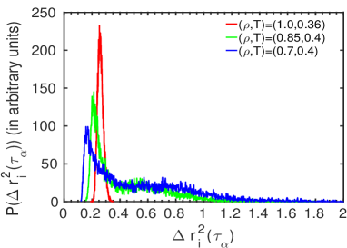
Figure 7: Probability distribution of squared displacements of individual monomers, $P[{\Delta r_{i}}^{2}(\tau_{\alpha})]$, averaged over time difference $t=\tau_{\alpha}$, at the lowest temperatures of the study where violation of the SE relation is pronounced.

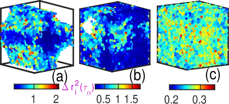
Figure 8: Squared displacement of each monomer at $t=\tau_{\alpha}$, i.e., $\Delta r_{i}^{2}(\tau_{\alpha})$ of (a) density $\rho=$ 0.7 at $T=$ 0.4, (b) density $\rho=$ 0.85 at $T=$ 0.4, and (c) density $\rho=$ 1.0 at $T=$ 0.36. Color bars are according to $\Delta r_{i}^{2}(\tau_{\alpha})$.

To examine the mobility of the particles in the system, we compute squared displacement of each particle (monomer), i.e.,

$${\Delta r_{i}}^{2}(\tau_{\alpha})=\langle|\mathbf{r}_{i}(\tau_{\alpha})-\mathbf{r}_{i}(0)|^{2}\rangle,$$ (9)

which is averaged over the time difference, $t=\tau_{\alpha}$, not over the particles. The probability distribution of ${\Delta r_{i}}^{2}(\tau_{\alpha})$, displayed in Fig. 7, shows a distribution of squared displacements at time $t=\tau_{\alpha}$ (average cage-relaxation time of monomers). Figure 7 shows that ranges of ${\Delta r_{i}}^{2}(\tau_{\alpha})$ are 0.13–2.1 and 0.16–1.7, respectively for $\rho=$ 0.7 and 0.85, at $T=$ 0.4, whereas ${\Delta r_{i}}^{2}(\tau_{\alpha})$ varies as 0.19–0.35 for the higher density at $T=$ 0.36, showing a significant difference in the range of $P[{\Delta r_{i}}^{2}(\tau_{\alpha})]$. Interestingly, $P[{\Delta r_{i}}^{2}(\tau_{\alpha})]$ of both lower density systems shows a hump (in addition to the main peak), which corresponds to the monomers that are faster than the average motion of the monomers in the system. Thus, it shows a disparity in ${\Delta r_{i}}^{2}(\tau_{\alpha})$ of monomers in both lower density systems compared to the higher density system where the range of ${\Delta r_{i}}^{2}(\tau_{\alpha})$ is narrow and no hump is present. For getting the spacial distribution of square displacements, we show the configurations of the systems with their squared displacements as a color map in Figs. 8(a) and 8(b), where both lower density systems show macroscopic cavities, however, the higher density system shows a continuous density distribution across the system [see Figs. A.2(a–c) for average nearest-neighbor distributions]. In both lower density systems at $T=$ 0.4, the monomers near the cavities show larger squared displacements at $t=\tau_{\alpha}$, whereas the monomers in the core show smaller squared displacements, i.e., the monomers in the core start freezing, whereas the monomers near the cavities are in the gaseous phase, which creates a disparity in their squared displacements resulting in the pronounced dynamic heterogeneity Royall and Williams (2015) in both lower density systems. The dynamical heterogeneity is less pronounced in $\rho=$ 0.85 system than the $\rho=$ 0.7 system because of a bit narrower distribution of the squared displacements at $t=\tau_{\alpha}$, as the surface of the cavities is reduced. This analysis suggests that an extent of the dynamical heterogeneity in the monomer motion of both lower densities arises due to a large disparity in their displacements because of the presence of surfaces around the cavities Singh and Jose (2019). As $P[{\Delta r_{i}}^{2}(\tau_{\alpha})]$ shows disparity in the distribution, we look at more averaged probability distributions, later in this study, thus attempt to correlate the SE violation with the observed disparity in the mobility. Now, it is interesting to look at the characterization of dynamic cages from the analysis of single particle motion, averaged over time differences and number of particles.

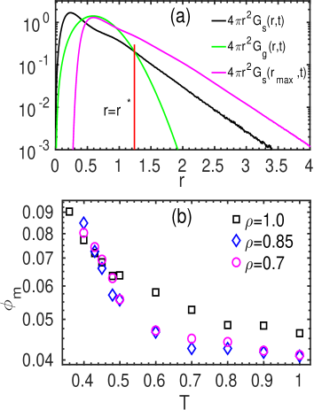
Figure 9: van Hove correlation function $G_{s}(r,t)$, its Gaussian approximation $G_{g}(r,t)$, and probability of maximum displacements $G_{s}(r_{max},t)$, are compared at time $t=\tau_{\alpha}$ for $\rho=$ 0.7 at $T=$ 0.4 (a). A variation in a fraction of mobile particles with temperature at densities $\rho=$ 1.0, 0.85, and 0.7 (b). Mobile particles are characterized as the particles that are moved greater than the distance $r^{*}$ at time $t$.

Jumplike motion of the particles in the system can be identified by self part of van Hove correlation function Hansen and McDonald (2006); Wahnstrom (1991); Sastry et al. (1998); Marcus et al. (1999); Kawasaki and Onuki (2013); Lam (2017),

$$G_{s}(\mathbf{r},t)=\frac{1}{N}\left\langle{\sum\limits_{i=1}^{N}{\delta[\mathbf{{r}}+{\mathbf{r}}_{i}(0)-{\mathbf{r}}_{i}(t)]}}\right\rangle.$$ (10)

The long tail in the $G_{s}(r,t)$ corresponds to the particles having larger displacements, thus, higher mobility. To calculate a cutoff radius $r$ and a fraction of these higher mobility particles, we compare the $G_{s}(r,t)$ with its Gaussian approximation at the same time, i.e., $\tau_{\alpha}$

$$G_{g}(r,\tau_{\alpha})=\left[\frac{3}{2\pi\langle r^{2}(\tau_{\alpha})\rangle}\right]^{3/2}\exp\left[\frac{-3r^{2}}{2\langle r^{2}(\tau_{\alpha})\rangle}\right],$$ (11)

which is displayed in Fig. 9(a). Here, $\langle r^{2}(\tau_{\alpha})\rangle$ is an average MSD of the monomers in the time interval [t, t+$\tau_{\alpha}$]. $G_{s}(r,t)$ is Gaussian in the ballistic time regime and in the diffusive time regime. Between these two time scales, it deviates from its Gaussian approximation given in Eq. 11. For comparison of $G_{s}(r,t)$ and $G_{g}(r,t)$, we choose to show (for example) the lower density $\rho=$ 0.7 at temperature $T=$ 0.4, which is shown in Fig. 9(a). We consider a particle as mobile if it travels a distance equal to or greater than $r^{*}$. The distance $r^{*}$ is marked by the red line in Fig. 9(a), where $G_{s}(r,t)$ crosses over to the $G_{g}(r,t)$. Thus, the fraction of mobile particles is computed as

$$\phi_{m}=\int_{r^{*}}^{\infty}4\pi r^{2}G_{s}(r^{*},\tau_{\alpha})dr,$$ (12)

as for e.g. in the binary LJ mixture Donati et al. (1999); Kob et al. (1997). In the previous studies of glass transition properties on the binary LJ mixture Donati et al. (1999); Kob et al. (1997) and polymers Starr et al. (2013), the fraction of mobile particles is calculated at a time scale corresponding to a peak value of the non-Gaussian parameter. Here, we choose the time scale as $t=\tau_{\alpha}$ for the calculation of a fraction of mobile particles because $\tau_{\alpha}$ is dominated by caged particles. However, the diffusion coefficient is dominated by mobile particles. Therefore, the estimation of mobile particles’ fraction at time $t=\tau_{\alpha}$ can give information about the decoupling between $D$ and $\tau_{\alpha}$. Figure 9(b) shows a variation in the fraction of mobile particles, $\phi_{m}$, with $T$ and $\rho$ : $\phi_{m}$ increases with $T$ from 4% to 9%, at each density. In the temperature range $T=$ 1.0–0.6, $\phi_{m}$ is around $\approx$ 4% and 5% for both lower densities and the higher density, respectively. However, in the supercooled regime ($T=$ 0.5–0.36), $\phi_{m}$ increases rapidly with a decrease in $T$, for all three densities, though it does not show a systematic variation with density. In Sec. III.3, we show that the SE violation increases with a decrease in the density at the same $T$. Thus, $\phi_{m}$ does not correlate with the extent of SE violations and the density of the system. This prompts us to look for a distribution function of the maximum displacement of the particles.

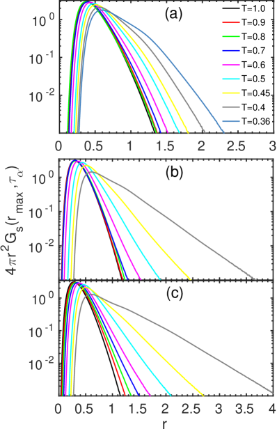
Figure 10: $4\pi r^{2}G_{s}(r_{max},\tau_{\alpha})$ of monomers is plotted against radial distance $r$ at densities (a) $\rho=$ 1.0, (b) $\rho=$ 0.85, and (c) $\rho=$ 0.7. The legend of (a) is applicable to (b) and (c).

As particles execute random walk (at the time scale of molecular diffusion) they revisit their original position, thus, the maximum distance a particle travels during a time interval $t$ is not identified in the $G_{s}(r,t)$. To identify the distribution of maximum displacement, we compute maximum displacement of a particle within a time interval [t, t+t^′], and then calculate its probability distribution similar to the $G_{s}(r,t)$. We use the definition of maximum displacement given in Ref. Kob et al. (1997),

$$r_{max}(t,\tau_{\alpha})=\textnormal{max}\{|\mathbf{r}(t+t^{\prime})-\mathbf{r}(t)|\},$$ (13)

where $t^{\prime}\in[0,\tau_{\alpha}]$. A probability distribution of $r_{max}(t,\tau_{\alpha})$, i.e., $4\pi r^{2}G_{s}(r_{max},\tau_{\alpha})$ is calculated and displayed in Figs. 10(a–c) to look at a variation in the mobility of particles with $T$ and $\rho$. This definition of mobility captures both type of particles, i.e., mobile particles, and most and least immobile particles. The long tail of $4\pi r^{2}G_{s}(r_{max},\tau_{\alpha})$ corresponds to the mobile particles. A systematic spread in $4\pi r^{2}G_{s}(r_{max},\tau_{\alpha})$ with temperature shows a difference in different mobilities of particles for all three densities, which measures the disparity in particles’ displacements. In the supercooled regime, the spread in the tail of $4\pi r^{2}G_{s}(r_{max},\tau_{\alpha})$ is more in both lower density systems compared to the higher density system, showing more disparity in the particles’ displacements. In Sec. III.3, we have shown that the SE violations are more pronounced in both lower density systems compared to the higher density system at the same $T$. Thus, the disparity in the particles’ motion is highly correlated with the violation of the SE relation in these linear polymer chains, instead of only the fraction of mobile particles. Furthermore, we show that the SE violations vary with the system size, which is related to the disparity in the particles’ mobility (see F for a detailed explanation). Next, we present the caging and jumplike motion of the particles, directly from their translational trajectories.

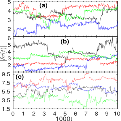
Figure 11: Trajectories of the monomer displacements, $|\delta\vec{r}(t)|=|\vec{r}_{i}(t)-\vec{r}_{i}(0)|$ for (a) $\rho=$ 1.0 at $T=$ 0.36, (b) $\rho=$ 0.85 at $T=$ 0.4, (c) $\rho=$ 0.7 at $T=$ 0.4. Different colors in (a), (b), and (c) correspond to the randomly selected monomers of different polymer chains.

In the supercooled regime, due to the presence of molecular cages, these molecules undergo large directed displacements by translation to escape from the self-generated barriers, thus relaxing the accumulation of the stress due to hindered motion. To identify such motions, we plot typical trajectories of the displacements of the randomly selected single monomers $|\mathbf{r}_{i}(t)-\mathbf{r}_{i}(0)|$ against time $t$ at the lowest temperatures $T=$ 0.4 and 0.36 to see whether there are large displacements in the monomers. Figures 11(a–c) show the typical trajectories of $\rho=$ 0.7 and 0.85 system at $T=$ 0.4, and $\rho=$ 1.0 system at $T=$ 0.36. These trajectories show the intermittent large displacements in the motion of monomers that have deviations from the regular random walk. Jumplike motions are difficult to identify in polymer systems with longer chains. An earlier study using continuous-time random walk on shorter chains ($n=$ 4) identifies jumps in the supercooled linear polymer melt Helfferich et al. (2014). However, jump like motions are found in several studies of glass-forming binary LJ systems (see Refs. Berthier and Biroli (2011); Bhattacharyya and Bagchi (2002)). These intermittent large displacements of the monomers are related to the fluctuations in the molecular configurations, which appear at the same state points where the violation of the SE relation is much pronounced, i.e., at $T=$ 0.4 and 0.36 for the lower density and higher density systems, respectively.

III.5 Violation of Stokes-Einstein-Debye relations

Polymers are extended macromolecules that have rotational degrees of freedom along with translational ones. The average rotational motion of polymer molecules can be quantified from the rotation of the unit vector along the end-to-end vector. The relaxation time of the rotational motion is calculated as $\tau_{l}=\int_{0}^{\infty}C_{l}^{r}(t)dt$, where $C_{l}^{r}(t)=\langle{P_{l}}[\cos\theta(t)]\rangle$ is $l^{th}$ order rotational correlation function for a non-spherical molecules Berne and Pecora (2000). Here, $\cos\theta(t)=\mathbf{\hat{e}}(0).\mathbf{\hat{e}}(t)$, and $\mathbf{\hat{e}}(t)$ is an unit vector along an end-to-end vector $\mathbf{e}(t)=\mathbf{r}_{1}(t)-\mathbf{r}_{n}(t)$ of a polymer chain; ${P_{l}}[\cos\theta(t)]$ is the Legendre polynomial of order $l$. Molecular liquids show translation-rotation coupling at high temperatures and obey the relation $D\tau_{l}=$ constant, which means that $D\propto\tau_{l}^{-1}$. Many studies show that near the glass transition the translation-rotation relaxation dynamics is decoupled Chong and Kob (2009); Stillinger and Hodgdon (1994). The failure of SED relation is usual in the molecular liquids Turton and Wynne (2014), which is much more pronounced in the orientatinal glasses, e.g., see Refs. Chong and Kob (2009); Jose et al. (2006). The polymer model, we have used in this study, is a non-polar, therefore, we have computed orientational relaxation time, especially, $\tau_{2}$ due to up-down symmetry, to examine the SED violation Andreozzi et al. (1996); Griffin et al. (2013). Recently, dependency of SED relation on the degree of Legendre polynomial, $l$, is examined by Kawasaki and Kim in supercooled water Kawasaki and Kim (2019). Data of $D$ vs $\tau_{2}$ is fitted with the relation $D\sim\tau^{-\xi}_{2}$, as shown in Fig. 12, and the variation of $\tau_{2}$ with temperature is shown in Fig. A.6. In both lower density systems, exponent $\xi=$ 1.0 from $T=$ 2.0–0.6, whereas in the supercooled regime ($T=$ 0.5–0.4), the exponent $\xi=$ 0.92 and $\xi=$ 0.78, respectively for $\rho=$ 0.85 and $\rho=$ 0.7 system. These fractional values of $\xi$ show a weak decoupling in $D$ and $\tau_{2}$ near $T_{c}$ in both lower density systems, which is significant in the $\rho=$ 0.7 system. On the other hand, in the higher density system, $\xi=$ 1.0 from high to low temperatures (up to $T=$ 0.36), which means that $D$ and $\tau_{2}$ are coupled even near the $T_{c}$.

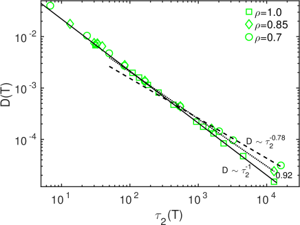
Figure 12: Diffusion coefficient $D(T)$ is plotted against $\tau_{2}(T)$. Solid, dotted, and dashed lines are fit to the data at densities $\rho=$ 1.0, 0.85, and 0.7, respectively; the data is fitted using relation $D\sim\tau^{-\xi}_{2}$.

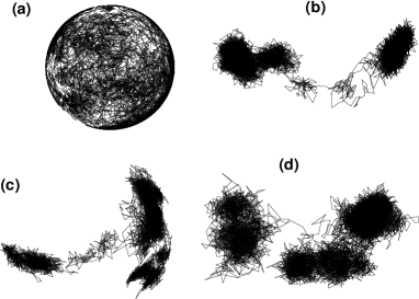
Figure 13: The trajectory of unit vector along the end-to-end vector of a randomly selected chain of the system for the time interval $\delta t=$ 2500. (a) $\rho=$ 0.85 at $T=$ 1.0, (b) $\rho=$ 0.85 at $T$ = 0.4, (c) $\rho=$ 1.0 at $T$ = 0.4, and (d) $\rho=$ 1.0 at $T$ = 0.36.

Analogous to the ratios of predictors of SE relation, we compute ratio of $D\tau_{2}=$ constant as a predictor for the SED violation Tarjus and Kivelson (1995) . The value of $D\tau_{2}$ is scaled with its value at $T=$ 1.0, which is shown in Fig. 6(c) (ratio is defined as $D\tau_{2}(T)/D\tau_{2}(T=1.0)$). In both lower density systems, this ratio starts from 1.0 and fluctuates around this value from $T=$ 0.9 to $T=$ 0.6. It starts increasing from $T=$ 0.5 and reaches around values 1.3 and 2.0 (at $T=$ 0.4) for $\rho=$ 0.85 and $\rho=$ 0.7 systems, respectively. This shows that SED relation is weakly violated in $\rho=$ 0.85 system, similar to the molecular SE violations, whereas violation is more for the $\rho=$ 0.7 system. In the temperature range where there is a maximum value of SED ratio, the exponent $\xi$ reduces, thus shows a correlation between them. In the higher density system, the SED ratio fluctuate close to 1.0 except at the lowest temperature $T=$ 0.36, where the ratios attains a value around 0.8. This implies that SED relation is valid in the higher density system even near $T_{c}$. An experimental and theoretical study by Gupta et al. shows that the Stokes-Einstein relation obeys up to the glass transition in starlike micelles owing to ultrasoft interactions Gupta et al. (2015) . Further, the translation-rotation decoupling is examined by the ratio of center of mass density relaxation time, calculated from $F_{s}^{C}(k,t)$, to the rotational relaxation time as $\tau_{2R_{g}}/\tau_{2}$ scaled with its value at $T=$ 1.0 [see Fig. 6(d)]. Similar to the ratio $D\tau_{2}$, the ratio $\tau_{2R_{g}}/\tau_{2}$ and $D\tau_{2R_{g}}$ also oscillate around 1.0 (all these values are scaled with their corresponding value at $T=$ 1.0), which means that translational molecular relaxation time and rotational relaxation time are coupled in the higher density system. However, the ratio $\tau_{2R_{g}}/\tau_{2}$ starts increasing from $T=$ 0.9 and reaches around a value 1.25 for $\rho=$ 0.85 and $\rho=$ 0.7, at the low temperature $T=$ 0.4. This shows a weak decoupling between $\tau_{2R_{g}}$ and $\tau_{2}$ in both lower density systems. Such decoupling was also found in an experimental study by Edmond et al. Edmond et al. (2012) in a colloidal glass, and a simulation study of glassy dumbbells Chong and Kob (2009). We expect a strong violation of SE and SED relations in our system, if the observed trend is continued below $T_{c}$.

As many studies show that the violation of SED relation is attributed to the enhanced hopping process in the rotational motion Michele and Leporini (2001b). Therefore, we look into the typical trajectory of an orientation vector $\boldsymbol{\hat{e}}(t)$ over the unit sphere of a few randomly selected polymer chains. In Fig. 13, we compare the rotation of $\boldsymbol{\hat{e}}(t)$ of polymer chains at one higher temperature and two lower temperatures. At $T=$ 1.0 of the density $\rho=$ 0.85, the trajectory of $\boldsymbol{\hat{e}}(t)$ [see Fig. 13(a)] shows a random walk, which uniformly spans over the sphere. However, the higher and lower density systems at the low temperatures [see Figs. 13(b–d)], show an intermittent motion of the rotational vector, which is a bit pronounced in the lower density systems. Figure 13(d) shows a trajectory of a randomly selected chain of the higher density system, which shows weak confinement at $T=$ 0.36. Earlier studies by Jose et al. show the pronounced violation of SED relation in nematogens during isotropic to nematic transition, which is due to the strong confinement of nematic ordering in the orientation of the molecules Jose et al. (2005, 2006). Such confinements at specified orientations are absent in this system. As polymer molecules are short chains, which are nearly spherically symmetric, and require more confinement to show SED violation.

IV Concluding remarks

The violations of Stokes-Einstein and Stokes-Einstein-Debye relations are defining characteristics of the glass transition, which are explained in terms of dynamic heterogeneities arise due to jumplike motions of mobile particles, and dynamic caging of immobile particles in simulations of atomistic model glass-formers Berthier et al. (2011). Another important class of glass-forming liquids is polymers that are difficult to crystallize. Direct observation of violation of SE and SED relations in simulations of model polymers are rare because of connectivity through the bonds between monomers, and the microscopic processes such as jumplike motions are difficult to detect Helfferich et al. (2014). However, the indirect observation of microscopic origins of violations of SE relation is examined in the earlier studies Puosi and Leporini (2012); Puosi et al. (2018). Due to extended shape of the polymers, we widen our study of the supercooled polymers near the glass transition to the lower density systems, where available volume for polymer chains is abundant, especially near the surface of dilute gas and supercooled liquid domains coexistence. Extensive molecular dynamics simulations of a linear Lennard-Jones polymer chains are performed at monomer number densities $\rho$ = 0.7, 0.85, and 1.0 from $T=$ 2.0–0.36. For the first two densities, the system forms domains of dilute gas and supercooled liquid, whereas the higher density system is homogeneous near the glass transition temperature $T_{c}$. Monomer density relaxation properties from the $F_{s}(k,t)$ at different time origins in the supercooled phase coexistence compared with that at $\rho=$ 1 at the same temperature show that the density relaxation is independent of the time origin in the systems where dilute gas and supercooled liquid coexist near the glass transition. The collective relaxation properties obtained from $G_{d}(r,t)$ shows that the gas-supercooled-liquid domains are stable within our simulation time. In these systems that differ in their density, we look for direct evidence of SE violation in the density relaxation of monomers and center of mass of polymer chains, and the SED violation of the polymer chains, near their MCT glass transition temperatures.

We show that monomer SE relation is violated for all three systems in the supercooled regime, which is pronounced in both lower density systems. The pronounced violation of the SE relation in both lower density systems is caused by the structural inhomogeneities and resulting dynamical heterogeneity due to the enhanced disparity in the monomer mobility in comparison to the higher density system. In the temperature range $T=$ 2.0–0.6, the molecular SE relation is obeyed in the higher and both lower density systems. However, in the supercooled regime, the higher density system obeys the molecular SE relation, whereas both lower density systems weakly violate it. At the lowest temperature of all three densities, we identify a hump at $r=\sigma$ and a peak at small $r$ in $G_{s}(r,t)$ that together show the monomer cages and jumplike motions in the monomer movement, which was also shown in the earlier studies of glass-forming binary mixtures Becker et al. (2006); Pan et al. (2017). Further, our study shows that disparity in the mobility of the monomers caused by the structural inhomogeneities is more in both lower density systems compared to the higher density system. Thus, we show that violations in the monomer and molecular SE relations are attributed to the presence of mobile and immobile particles, the jumplike motions, and caging in this linear polymer system at temperatures near $T_{c}$. We also show that the unit vector associated with the polymer chains undergoes confinement. Thus, there is a weak violation in the SED relation for both lower density systems, supported by the intermittent motion found in the typical trajectory of the end-to-end unit vector. Our study also shows that the glass transition in the presence of static structural inhomogeneities is very much similar to the continuous phases. Many aspects of the formation of the glassy domains in the model glassy binary mixtures are studied in the simulations Testard et al. (2011); Varughese and Jose (2016) and experiments Tanaka et al. (2005); Cardinaux et al. (2007); Godfrin et al. (2018), where glass transition and phase separation coexist, though the inter-molecular potentials and molecular geometry are different from our study. Therefore, the simulations with more model potentials and varying range of attractions are required for obtaining the quantitative information about the microscopic glassy domains formed in the phase separating systems.

Appendix A Radius of gyration

The size of polymer chains can be measured from the calculation of radius of gyration. The equilibrium average mean square radius of gyration is

$${R^{2}_{g}}={\frac{1}{n}}\left\langle\sum\limits_{i=1}^{n}{{({\mathbf{R}}_{i}-{\mathbf{R}}_{cm})}^{2}}\right\rangle,$$ (14)

where ${\mathbf{R}}_{cm}={\frac{1}{n}}\sum\limits_{i=1}^{n}{{\mathbf{R}}_{i}}$ is a position of the center of mass of a chain and ${\mathbf{R}}_{i}$ is the position vector of $i$th monomer and $n$ is the total number of monomers in a chain Doi and Edwards (1986). We show that (flexible) polymer chains are nearly Gaussian as $R_{g}^{2}\simeq R_{e}^{2}/6$ (see Fig. A.1), partially because the chains are short therefore they are confined to an average small radius. Here, $R_{g}^{2}$ and $R_{e}^{2}$ are respectively radius of gyration and end-to-end distance squares. Calculations presented here show that the radius of gyration changes with temperature by $\sim$ 2% in the higher density system and $\sim$ 3% in both lower density systems.

Appendix B Local packing of monomers

Figure 8 and our previous study of this system Singh and Jose (2019) show that lower density systems phase separate at low temperatures. To examine a variation of the local density with temperature in the phase separating systems, we calculate local packing of the monomers in the linear polymer system at three different densities. The local packing is obtained from the calculation of number of nearest neighbors $N_{b}$ of each monomer in the first coordination shell (FCS), which is at 0 $<r\leq r_{fcs}$; $r_{fcs}=$ 1.5 is a position of the first minima of the radial distribution function of the system Singh and Jose (2016, 2019) . Using this FCS radius, its volume can be calculated as $V_{fcs}=(4/3)\pi r_{fcs}^{3}=$ 14.137, which subsequently gives the local density $\rho_{l}=(N_{b}+1)/V_{fcs}$. Figure A.2 shows that range of $N_{b}$ is 3–18 at $T=$ 0.4 for $\rho=$ 0.7 and 0.85, whereas $N_{b}=$ 9–18 at $T=$ 0.36 of the higher density system. Thus, the local density range is calculated as $\rho_{l}=$ 0.283–1.344 at $T=$ 0.4 of the lower densities $\rho=$ 0.7 and 0.85, and $\rho_{l}=$ 0.707–1.344 at $T=$ 0.36 of the higher density system. This variation in the local density range shows a coexistence of dilute gas and dense amorphous domains in both lower density systems at temperatures near $T_{c}$.

Further, the nearest neighbor distribution averaged over the steady-state configurations [given in Figs. A.2(a–c)] shows that the higher density system does not show macroscopic cavities, whereas both lower density systems show cavities as temperature reduces, resulting in the structural inhomogeneities Singh and Jose (2019). In both lower densities [see Figs. A.2(a) and A.2(b)], major peak of $P(N_{b})$ shifts to $N_{b}=$ 13 and 14 at low temperatures, whereas in the higher density system [see Fig. A.2(c)], the peak height grows at $N_{b}=$ 13 and 14 from high to low temperatures. Thus, the packing of the monomers that are inside the dense domains are similar for all three densities because of the monomers within the dense domains in both lower density systems have the same range of $N_{b}$ to that the higher density system. At low temperatures, a hump in $P(N_{b})$ at $N_{b}\simeq$ 8–10 is appearing in both lower density systems, which is absent in the higher density system. This hump in $P(N_{b})$ confirms the structural inhomogeneity in both lower density systems, however, an approximately equal peak height at $N_{b}=$ 13 and 14 indicates the similarity in the local packing of the dense glassy domains in all three systems at low temperatures.

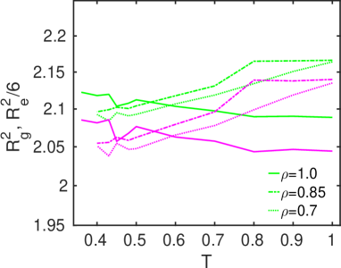
Figure A.1: Average squared radius of gyration $R^{2}_{g}$ (green) and $R^{2}_{e}/6$ (magenta) of $\rho=$ 0.7, 0.85, and 1.0 systems are plotted against temperature $T$.

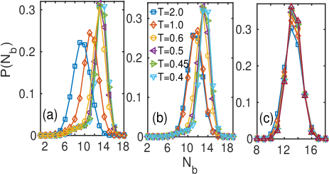
Figure A.2: Average probability distribution $P(N_{b})$ is plotted against $N_{b}$ at $T=$ 2.0–0.36: (a) $\rho=$ 0.7, (b) $\rho=$ 0.85, and (c) $\rho=$ 1.0. In (a) and (b), $P(N_{b})$ shows nonzero values for the smaller $N_{b}$, which corresponds to the gas-liquid phase coexistence at high temperatures. The liquid phase becomes amorphous solid-like coexisting with the gaseous particles at low temperatures.

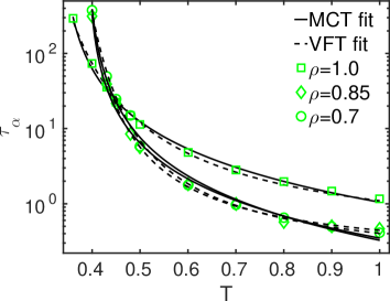
Figure A.3: Fitting of $\alpha-$relaxation time with the MCT and VFT relations. Note that the VFT relation is a good fit to the data.

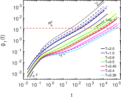
Figure A.4: Mean squared displacement of monomers is plotted against time $t$. Solid, dashed, and dotted lines are corresponding to the densities $\rho=$ 1.0, 0.85, and 0.7 respectively.

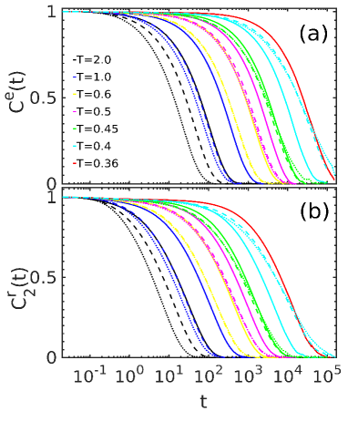
Figure A.5: End-to-end vector time correlation function (a) and Relaxation of second order time correlation function of the rotational vector (b) of polymer chains. Solid, dashed, and dotted lines are corresponding to $\rho=$ 1.0, 0.85, and 0.7.

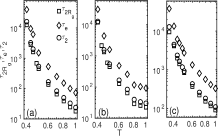
Figure A.6: Molecular relaxation times $\tau_{2R_{g}}$, $\tau_{e}$, and $\tau_{2}$ are plotted against temperature $T$ at densities (a) $\rho=$ 0.7, (b) $\rho=$ 0.85, and (c) $\rho=$ 1.0.

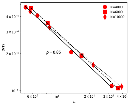
Figure A.7: Diffusion coefficient $D(T)$ is plotted against monomer $\alpha-$relaxation time at different system sizes, in the range of temperatures ($T=$ 0.5–0.43) where the SE relation is violated. Data is fitted with the fractional SE relation, i.e., $D\propto\tau^{-\xi}$. Solid, dashed, and dotted lines are fit to the data corresponding to $N=$ 4000, 6000, and 10000. The corresponding exponents are 0.83, 0.82, and 0.73.

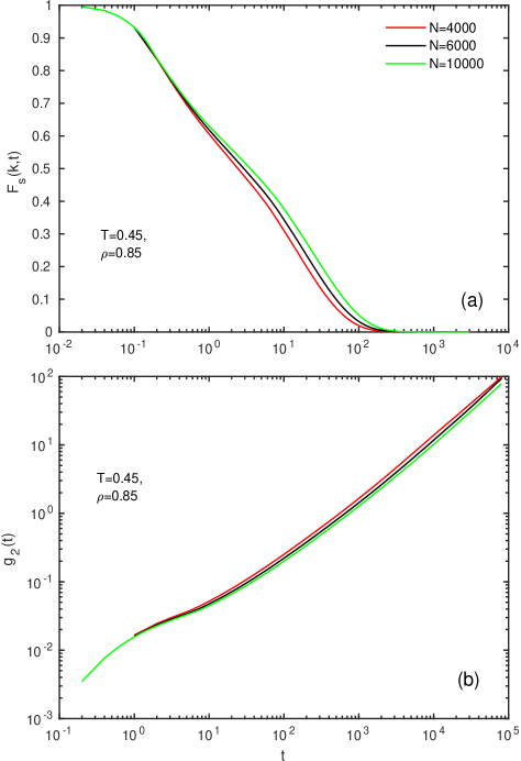
Figure A.8: Slow dynamics of different system sizes at one representative temperature $T=$ 0.45. (a) $F_{s}(k,t)$ and (b) Center of mass MSD, $g_{2}(t)$. This shows that $F_{s}(k,t)$ and center of mass MSD slow down as the system size increases.

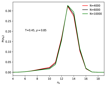
Figure A.9: Nearest neighbor distribution, $P(n_{b})$ at different system sizes of one representative temperature $T=$ 0.45. $P(n_{b})$ at low $n_{b}$ decreases whereas it increases at $n_{b}=$ 14, with the system sizes.

Appendix C Relaxation time and the fitting

The monomer $\alpha-$relaxation times are plotted against temperature $T$ in Fig. A.3 at three different densities. The $\tau_{\alpha}$ vs $T$ curves are fitted with the MCT and VFT relations and described in the main text. The $\alpha-$relaxation time is longer for the higher density system compared to both lower density systems up to $T=$ 0.45. At $T=$ 0.4, the $\alpha-$relaxation time of both lower densities show a crossover to the higher density system, which is also evident from the slower decay of the $F_{s}(k,t)$.

Appendix D Monomer mean-squared displacement

An average squared displacement of a particle from its initial position can be calculated from its mean-squared displacement (MSD)

$$g_{1}(t)=\langle\left[\mathbf{r}(0)-\mathbf{r}(t)\right]^{2}\rangle,$$ (15)

which is shown in Fig. A.4 at various temperatures of the three different densities. Figure A.4 shows that monomers show the ballistic motion ($\sim t^{2}$) at a short time, crossing over to the intermediate caging regime ($\sim t^{\alpha}$, $0<\alpha<1$) owing to various interactions, bonding as well as non-bonding type. There exists a sub-diffusive regime in the MSD of monomers after the caging regime, which is due to the chain hindrance and varies with power-law $g_{1}(t)\sim t^{0.63}$ Barrat et al. (2010). Finally, the diffusive regime in the monomer MSD starts from time $t\sim 10^{3}$ at the temperature $T=$ 2.0, whereas at lowest temperatures ($T=$ 0.4 and $T=$ 0.36) the diffusive regime starts at the time scale of $t\sim 10^{6}$ Barrat et al. (2010). As the temperature of the system gets lowered the caging of the monomer MSDs becomes more pronounced, which is supported by the $F_{s}(k,t)$ shown in the main text. The monomer MSD of the higher density system is slower than both lower density systems above $T=$ 0.4, shows a crossover at $T=$ 0.4 where the monomer MSD of both lower density systems becomes slower.

Appendix E Orientation

Further understanding of the molecular relaxation is obtained from the rotational motion of the polymer chains. An autocorrelation function of the End-to-end vector is defined as Doi and Edwards (1986)

$$C^{e}(t)=\frac{\left\langle\mathbf{e}(0).\mathbf{e}(t)\right\rangle}{\left\langle\mathbf{e}(0).\mathbf{e}(0)\right\rangle},$$ (16)

which gives a detail of the molecular shape relaxation in the polymers. Figure A.5(a) shows the $C^{e}(t)$ of polymer chains at different temperatures of three densities. The relaxation of $C^{e}(t)$ is slower with an increase in the density at temperatures $T=$ 2.0 and 1.0. Below these temperatures, the relaxation of $C^{e}(t)$ becomes identical for both lower densities. However, $C^{e}(t)$ of the higher density system decays slower than both lower density systems up to $T=$ 0.45. A crossover in the relaxation time of both lower density systems appears at $T=$ 0.4, and $C^{e}(t)$ relaxes slowly. We have computed the time constant for end-to-end vector relaxation at all temperatures, which is defined as $\tau_{e}=\int_{0}^{\infty}C^{e}(t)dt$. A variation in $\tau_{e}$ with $T$ is plotted in Fig. A.6 at three different densities, which is qualitatively similar to the $C^{e}(t)$. The relaxation of $C^{e}(t)$ has contributions from the rotation as well as shape fluctuations of the polymer chains, thus we compute rotational correlation functions.

The rotational relaxation time is quantified from the rotational correlation function $C_{l}^{r}(t)$ for a non-spherical molecule Berne and Pecora (2000). Hydrodynamic SED model of rotational relaxation predicts an exponential relaxation of $C_{l}^{r}(t)$, i.e., $C_{l}^{r}(t)=e^{-t/\tau_{l}}$ for liquids at high temperatures, where $\tau_{l}$ is the time constant of $l^{th}$ order orienational correlation function. The rotational correlation function, corresponding to $l=$ 2, i.e., $C_{2}^{r}(t)$, is plotted in Fig. A.5(b). The effect of density on the nature of the relaxation of $C_{2}^{r}(t)$ is similar to the $C^{e}(t)$, as described above. At high temperatures, $C_{2}^{r}(t)$ shows exponential relaxation as predicted by the SED model. However, at temperatures ($T=$ 0.45–0.4), $C_{2}^{r}(t)$ not only slows down but also shows an emergence of a shoulder, immediately after the fast initial decay. The appearance of the shoulder hints the formation of cages in the rotational motion of the polymer molecules due to the orientational confinement at small angles. These small-angle confinements are correlated to the confinement of rotational motion, shown in the trajectory of the unit vectors (see Fig. 13).

A comparison of variation in translational molecular relaxation time $\tau_{2R_{g}}$, end-to-end vector relaxation time $\tau_{e}$, and rotational relaxation times $\tau_{2}$ with temperature and density, is shown in Fig. A.6. All these relaxation times grow as temperature reduces for all three density systems, though they are higher for the higher density system up to $T=$ 0.45. A crossover in the relaxation times is also observed around $T=$ 0.4 for both lower density systems. Interestingly, these relaxation time at $T=$ 0.36 of the higher density system, reach near to the value at $T=$ 0.4 of both lower density systems.

Appendix F Finite-size effects

To examine finite-size effects due to cavities, we have studied two smaller size systems at the density $\rho=$ 0.85, consisting of $N=$ 4000 and 6000 number of particles (beads), and compared results with that of the system of $N=$ 10000 particles. A plot of $D$ vs $\tau_{\alpha}$ at different system sizes, given in Fig. A.7, shows that in all three systems the relaxation time increases with system size, and the diffusion coefficient decreases by a smaller factor, which results in a variation in the violation of the SE relation with system size. The exponent $\xi$ decreases with increasing system size, indicating that the larger system shows the larger violations. To analyze how relaxation time and diffusion vary with system size, the $F_{s}(k,t)$ of monomers and center of mass MSD of polymer molecules, at a representative temperature $T=$ 0.45, are compared at different system sizes in Figs. A.8(a-b), showing a slow down of strucutral relaxation with an increase of the system sizes. This observed variation can be associated with a change in the relative distribution of surface and bulk particles in the system; this is identified from the nearest-neighbor distribution, shown in Fig. A.9, where it shifts to the higher $n_{b}$ as the system size increases. This leads to the larger disparity in the mobility of particles, thus enhances the extent of the SE violations. It is expected that the finite-size effects may saturate at very large system sizes which may be worthwhile to address in future studies using simulations or experiments. As there is an enhancement of SE violations with system size, experiments that involve a larger number of particles are expected to show a more pronounced SE violations.

References

- Hansen and McDonald (2006) J. P. Hansen and I. R. McDonald, Theory of Simple Liquids (Academic Press, London, 2006).
- Stokes (1851) G. G. Stokes, Trans. Cambridge Philos. Soc. 9, 8 (1851).
- Einstein (1905) A. Einstein, Ann. Phys. 322, 549 (1905).
- Kawasaki and Kim (2017) T. Kawasaki and K. Kim, Sci. Adv. 3, e1700399 (2017).
- Sengupta et al. (2013) S. Sengupta, S. Karmakar, C. Dasgupta, and S. Sastry, J. Chem. Phys. 138, 12A548 (2013).
- Bhowmik et al. (2016) B. P. Bhowmik, R. Das, and S. Karmakar, J. Stat. Mech. , 074003 (2016).
- Shi et al. (2013) Z. Shi, P. G. Debenedetti, and F. H. Stillinger, J. Chem. Phys. 138, 12A526 (2013).
- Yamamoto and Onuki (1998) R. Yamamoto and A. Onuki, Phys. Rev. Lett. 81, 4915 (1998).
- (9) In liquids at high temperatures, intermediate incoherent scattering function can be given as Hansen and McDonald (2006), here, is a wave vector near the first peak of static structure factor . This suggests that constant, or constant, implies that , which according to constant, entails that .
- Becker et al. (2006) S. R. Becker, P. H. Poole, and F. W. Starr, Phys. Rev. Lett. 97, 055901 (2006).
- Puosi and Leporini (2012) F. Puosi and D. Leporini, J. Chem. Phys. 136, 211101 (2012).
- Pan et al. (2017) S. Pan, Z. W. Wu, W. H. Wang, M. Z. Li, and L. Xu, Sci. Rep. 7, 39938 (2017).
- Ediger (2000) M. D. Ediger, Ann. Rev. Phys. Chem. 51, 99 (2000).
- Andreozzi et al. (1996) L. Andreozzi, A. D. Schino, M. Giordano, and D. Leporini, J. Phys.: Condens. Matter 8, 9605 (1996).
- Edmond et al. (2012) K. V. Edmond, M. T. Elsesser, G. L. Hunter, D. J. Pine, and E. R. Weeks, Proc. Natl. Acad. Sci. 109, 17891 (2012).
- Mishra and Ganapathy (2015) C. K. Mishra and R. Ganapathy, Phys. Rev. Lett. 114, 198302 (2015).
- Berthier et al. (2011) L. Berthier, G. Biroli, J. Bouchaud, L. Cipelletti, and W. Saarloos, eds., Dynamical Heterogeneities in Glasses, Colloids and Granular Media (Oxford University Press, New York, 2011).
- Flenner et al. (2014) E. Flenner, H. Staley, and G. Szamel, Phys. Rev. Lett. 112, 097801 (2014).
- Donati et al. (1999) C. Donati, S. C. Glotzer, P. H. Poole, W. Kob, and S. J. Plimpton, Phys. Rev. E 60, 3107 (1999).
- Glotzer (2000) S. C. Glotzer, J. Non-Cryst. Solids 274, 342 (2000).
- Richert (2002) R. Richert, J. Phys.: Condens. Matter 14, R703 (2002).
- Kob et al. (1997) W. Kob, C. Donati, S. J. Plimpton, P. H. Poole, and S. C. Glotzer, Phys. Rev. Lett. 79, 2827 (1997).
- Charbonneau et al. (2014) P. Charbonneau, Y. Jin, G. Parisi, and F. Zamponie, Proc. Natl. Acad. Sci. 111, 15025 (2014).
- Chong (2008) S.-H. Chong, Phys. Rev. E 78, 041501 (2008).
- Zou et al. (2019) Q.-Z. Zou, Z.-W. Li, Y.-L. Zhu, and Z.-Y. Sun, Soft Matter 15, 3343 (2019).
- Kumar et al. (2006) S. K. Kumar, G. Szamel, and J. F. Douglas, J. Chem. Phys. 124, 214501 (2006).
- Debye (1929) P. Debye, Polar Molecules (Dover Publications, New York, 1929) p. 72.
- Berne and Pecora (2000) B. J. Berne and R. Pecora, Dynamic Light Scattering: With applications to Chemistry, Biology and Physics (Dover Publications, New York, 2000).
- Tarjus and Kivelson (1995) G. Tarjus and D. Kivelson, J. Chem. Phys. 103, 3071 (1995).
- Doi and Edwards (1986) M. Doi and S. F. Edwards, The theory of polymer dynamics (Clarendon Press, Oxford, 1986).
- de Gennes (1979) P. G. de Gennes, Scaling Concepts in Polymer Physics (Cornell University Press, Ithaca and London, 1979).
- Kirkwood (1954) J. G. Kirkwood, J. Polym. Sci. 12, 1 (1954).
- Rubinstein and Colby (2003) M. Rubinstein and R. H. Colby, Polymer physics (Oxford University Press, Oxford, 2003).
- Mansfield et al. (2015) M. L. Mansfield, A. Tsortos, and J. F. Douglas, J. Chem. Phys. 143, 124903 (2015).
- Clisby and Dünweg (2016) N. Clisby and B. Dünweg, Phys. Rev. E 94, 052102 (2016).
- Vargas-Lara et al. (2017) F. Vargas-Lara, M. L. Mansfield, and J. F. Douglas, J. Chem. Phys. 147, 014903 (2017).
- Costigliola et al. (2019) L. Costigliola, D. M. Heyes, T. B. Schrøder, and J. C. Dyre, J. Chem. Phys. 150, 021101 (2019).
- Ohtori and Ishii (2015) N. Ohtori and Y. Ishii, Phys. Rev. E 91, 012111 (2015).
- Ohtori et al. (2018) N. Ohtori, H. Uchiyama, and Y. Ishii, J. Chem. Phys. 149, 214501 (2018).
- Mazza et al. (2007) M. G. Mazza, N. Giovambattista, H. E. Stanley, and F. W. Starr, Phys. Rev. E 76, 031203 (2007).
- Ngai (1999) K. L. Ngai, Phil. Mag. B 79, 1783 (1999).
- Michele and Leporini (2001a) C. D. Michele and D. Leporini, Phys. Rev. E 63, 036701 (2001a).
- Michele and Leporini (2001b) C. D. Michele and D. Leporini, Phys. Rev. E 63, 036702 (2001b).
- Helfferich et al. (2014) J. Helfferich, F. Ziebert, S. Frey, H. Meyer, J. Farago, A. Blumen, and J. Baschnagel, Phys. Rev. E 89, 042603 (2014).
- Puosi et al. (2018) F. Puosi, A. Pasturel, N. Jakse, and D. Leporini, J. Chem. Phys. 148, 131102 (2018).
- Balbuena and Soul (2020) C. Balbuena and E. R. Soul, J. Phys.: Condens. Matter 32, 045401 (2020).
- Starr et al. (2002) F. W. Starr, S. Sastry, J. F. Douglas, and S. C. Glotzer, Phys. Rev. Lett. 89, 125501 (2002).
- Bennemann et al. (1998) C. Bennemann, W. Paul, K. Binder, and B. Dnweg, Phys. Rev. E 57, 843 (1998).
- Huang (2010) K. Huang, Introduction to Statistical Physics (CRC Press, Taylor & Francis Group, Boca Raton, FL, 2010).
- Foffi et al. (2005) G. Foffi, C. D. Michele, F. Sciortino, and P. Tartaglia, J. Chem. Phys. 122, 224903 (2005).
- Cardinaux et al. (2007) F. Cardinaux, T. Gibaud, A. Stradner, and P. Schurtenberge, Phys. Rev. Lett. 99, 118301 (2007).
- Godfrin et al. (2018) P. D. Godfrin, P. Falus, L. Porcar, K. Hong, S. D. Hudson, N. J. Wagner, and Y. Liu, Soft Matter 14, 8570 (2018).
- Chaudhuri and Horbach (2016) P. Chaudhuri and J. Horbach, Phys. Rev. B 94, 094203 (2016).
- Testard et al. (2011) V. Testard, L. Berthier, and W. Kob, Phys. Rev. Lett. 106, 125702 (2011).
- Priezjev and Makeev (2017) N. V. Priezjev and M. A. Makeev, Phys. Rev. E 96, 053004 (2017).
- Makeev and Priezjev (2018) M. A. Makeev and N. V. Priezjev, Phys. Rev. E 97, 023002 (2018).
- Grest and Kremer (1986) G. S. Grest and K. Kremer, Phys. Rev. A 33, 3628 (1986).
- Allen and Tildesley (1987) M. P. Allen and D. J. Tildesley, Computer simulation of liquids (Clarendon Press, Oxford, 1987).
- Kob and Barrat (1997) W. Kob and J.-L. Barrat, Phys. Rev. Lett. 78, 4581 (1997).
- Barrat et al. (2010) J.-L. Barrat, J. Baschnagel, and A. Lyulin, Soft Matter 6, 3430 (2010).
- Chong and Fuchs (2002) S.-H. Chong and M. Fuchs, Phys. Rev. Lett. 88, 185702 (2002).
- Angel (1995) C. A. Angel, Science 267, 1924 (1995).
- Li et al. (2019) Y.-W. Li, C. K. Mishra, Z.-Y. Sun, K. Zhao, T. G. Mason, R. Ganapathy, and M. P. Ciamarra, Proc. Natl. Acad. Sci. 116, 22977–22982 (2019).
- Puertas et al. (2007) A. M. Puertas, C. D. Michele, F. Sciortino, P. Tartaglia, and E. Zaccarelli, J. Chem. Phys. 127, 144906 (2007).
- Royall and Williams (2015) C. P. Royall and S. R. Williams, Phys. Rep. 560, 1 (2015).
- Singh and Jose (2019) J. Singh and P. P. Jose, AIP Conference Proceedings 2115, 030236 (2019).
- Wahnstrom (1991) G. Wahnstrom, Phys. Rev. A 44, 3752 (1991).
- Sastry et al. (1998) S. Sastry, P. G. Debenedetti, and F. H. Stillinger, Nature 393, 554 (1998).
- Marcus et al. (1999) A. H. Marcus, J. Schofield, and S. A. Rice, Phys. Rev. E 60, 5725 (1999).
- Kawasaki and Onuki (2013) T. Kawasaki and A. Onuki, Phys. Rev. E 87, 012312 (2013).
- Lam (2017) C.-H. Lam, J. Chem. Phys. 146, 244906 (2017).
- Starr et al. (2013) F. W. Starr, J. F. Douglas, and S. Sastry, J. Chem. Phys. 138, 12A541 (2013).
- Berthier and Biroli (2011) L. Berthier and G. Biroli, Rev. Mod. Phys. 83, 587 (2011).
- Bhattacharyya and Bagchi (2002) S. Bhattacharyya and B. Bagchi, Phys. Rev. Lett. 89, 025504 (2002).
- Chong and Kob (2009) S.-H. Chong and W. Kob, Phys. Rev. Lett. 102, 025702 (2009).
- Stillinger and Hodgdon (1994) F. H. Stillinger and J. A. Hodgdon, Phys. Rev. E 50, 2064 (1994).
- Turton and Wynne (2014) D. A. Turton and K. Wynne, J. Phys. Chem. B 118, 4600 (2014).
- Jose et al. (2006) P. P. Jose, D. Chakrabarti, and B. Bagchi, Phys. Rev. E 73, 031705 (2006).
- Griffin et al. (2013) P. J. Griffin, J. R. Sangoro, Y. Wang, A. P. Holt, V. N. Novikov, A. P. Sokolov, Z. Wojnarowska, M. Paluch, and F. Kremer, Soft Matter 9, 10373 (2013).
- Kawasaki and Kim (2019) T. Kawasaki and K. Kim, Nat. Comm. 9, 8118 (2019).
- Gupta et al. (2015) S. Gupta, J. Stellbrink, E. Zaccarelli, C. N. Likos, M. Camargo, P. Holmqvist, J. Allgaier, L. Willner, and D. Richter, Phys. Rev. Lett. 115, 128302 (2015).
- Jose et al. (2005) P. P. Jose, D. Chakrabarti, and B. Bagchi, Phys. Rev. E 71, 030701(R) (2005).
- Varughese and Jose (2016) A. Varughese and P. P. Jose, J. Phys.: Conf. Ser. 759, 012019 (2016).
- Tanaka et al. (2005) H. Tanaka, T. Araki, T. Koyama, and Y. Nishikawa, J. Phys.: Condens. Matter 17, S3195 (2005).
- Singh and Jose (2016) J. Singh and P. P. Jose, J. Phys.: Conf. Ser. 759, 012018 (2016).