How much faster does the best polynomial approximation converge than Legendre projection?

Abstract

We compare the convergence behavior of best polynomial approximations and Legendre and Chebyshev projections and derive optimal rates of convergence of Legendre projections for analytic and differentiable functions in the maximum norm. For analytic functions, we show that the best polynomial approximation of degree $n$ is better than the Legendre projection of the same degree by a factor of $n^{1/2}$. For differentiable functions such as piecewise analytic functions and functions of fractional smoothness, however, we show that the best approximation is better than the Legendre projection by only some constant factors. Our results provide some new insights into the approximation power of Legendre projections.

1 Introduction

The Legendre polynomials are one of the most important sequences of orthogonal polynomials which have been extensively used in many branches of scientific computing such as Gauss-type quadrature, special functions, $p$-version of the finite element method and spectral methods for differential and integral equations (see, e.g., canuto2006spectral ; davis1984methods ; eriksson1986error ; gui1986fem ; hesthaven2007spectral ; osipov2013pswf ; shen1994legendre ; shen2011spectral ; szego1975orthogonal ). Among these applications, Legendre polynomials are particularly appealing owing to their superior properties: (i) they have excellent error properties in the approximation of a globally smooth function; (ii) quadrature rules based on their zeros or extrema are optimal in the sense of maximizing the exactness of integrated polynomials; (iii) they are orthogonal with respect to the uniform weight function $\omega(x)=1$ which makes them preferable in Galerkin methods for PDEs.

Let $n\geq 0$ be an integer and let $P_{n}(x)$ denote the Legendre polynomial of degree $n$ which is normalized by $P_{n}(1)=1$. The sequence of Legendre polynomials $\{P_{n}(x)\}$ forms a system of polynomials orthogonal over $\mathrm{\Omega}=[-1,1]$ and

$$\int_{-1}^{1}P_{n}(x)P_{m}(x)\mathrm{d}x=\frac{2}{2n+1}\delta_{mn},$$ (1)

where $\delta_{mn}$ is the Kronecker delta (olver2010nist, , p. 14). Given a real-valued function $f(x)$ which belongs to a Lipschitz class of order larger than $1/2$ on $\mathrm{\Omega}$, then it has the following uniformly convergent Legendre series expansion suetin1964legendre

$$f(x)=\sum_{k=0}^{\infty}a_{k}P_{k}(x),\quad a_{k}=\left(k+\frac{1}{2}\right)\int_{-1}^{1}f(x)P_{k}(x)\mathrm{d}x.$$ (2)

Let $\mathcal{P}_{n}(f)$ denote the truncated Legendre expansion of degree $n$, i.e.,

$$\mathcal{P}_{n}(f)=\sum_{k=0}^{n}a_{k}P_{k}(x).$$ (3)

which is also known as the Legendre projection. It is well known that this polynomial is the best polynomial approximation to $f(x)$ in the $L^{2}$ norm with respect to the Legendre weight $\omega(x)=1$. The computation of the first $n+1$ Legendre coefficients $\{a_{k}\}_{k=0}^{n}$ has received much attention over the past decade and fast algorithms have been developed in alpert1991legendre ; iserles2011legendre that require only $O(n\log n)$ operations and in townsend2018fast that require $O(n\log^{2}n)$ operations.

Besides Legendre polynomials, another widely used sequence of orthogonal polynomials is the Chebyshev polynomials, i.e., $T_{k}(x)=\cos(k\arccos(x))$. Suppose that $f(x)$ is Dini-Lipschitz continuous on $\mathrm{\Omega}$, then it has the following uniformly convergent Chebyshev series (mason2003chebyshev, , Theorem 5.7)

$$f(x)=\sum_{k=0}^{\infty}{{}^{\prime}}c_{k}T_{k}(x),\quad c_{k}=\frac{2}{\pi}\int_{-1}^{1}\frac{f(x)T_{k}(x)}{\sqrt{1-x^{2}}}\mathrm{d}x,$$ (4)

where the prime indicates that the first term of the sum is halved. Let $\mathcal{T}_{n}(f)$ denote the truncated Chebyshev expansion of degree $n$, i.e.,

$$\mathcal{T}_{n}(f)=\sum_{k=0}^{n}a_{k}T_{k}(x),$$ (5)

which is also known as the Chebyshev projection. It is well known that $\mathcal{T}_{n}(f)$ is the best polynomial approximation to $f(x)$ in the $L^{2}$ norm with respect to the Chebyshev weight $\omega(x)=(1-x^{2})^{-1/2}$ and the first $n+1$ Chebyshev coefficients $\{c_{k}\}_{k=0}^{n}$ can be evaluated efficiently by making use of the FFT in only $O(n\log n)$ operations (see, e.g., (mason2003chebyshev, , Section 5.2.2)).

Let $\mathcal{B}_{n}(f)$ denote the best approximation polynomial of degree $n$ to $f$ on $\mathrm{\Omega}=[-1,1]$ in the maximum norm, i.e.,

$$\|f-\mathcal{B}_{n}(f)\|_{\infty}=\min_{p\in\mathrm{\Pi}_{n}}\|f-p\|_{\infty},$$

where $\mathrm{\Pi}_{n}$ denotes the space of polynomials of degree at most $n$. If $f$ is continuous on $\mathrm{\Omega}$, it is well known that $\mathcal{B}_{n}(f)$ exists and is unique. From the point of view of polynomial approximation in the maximum norm, it is clear that $\mathcal{B}_{n}(f)$ is more accurate than $\mathcal{P}_{n}(f)$ and $\mathcal{T}_{n}(f)$. However, explicit expressions for $\mathcal{B}_{n}(f)$ are generally impossible to obtain since the dependence of $\mathcal{B}_{n}(f)$ on $f$ is nonlinear and Remez-type algorithms, which are realized by iterative procedures, have been developed for computing $\mathcal{B}_{n}(f)$ (see, e.g., (trefethen2013atap, , Chapter 10)). Although algorithms are available, they are still time-consuming when $n$ is in the thousands or higher. Obviously, this leads us to face an inevitable dilemma of whether the increase in accuracy is sufficient to justify the extra cost of computing $\mathcal{B}_{n}(f)$.

With these three approaches, a natural question is: How much better is the accuracy of $\mathcal{B}_{n}(f)$ than $\mathcal{T}_{n}(f)$ and $\mathcal{P}_{n}(f)$ in the maximum norm? For the case of $\mathcal{T}_{n}(f)$ where $f\in C(\mathrm{\Omega})$, it has been shown in (rivlin1981approx, , Theorem 2.2) that the maximum error of $\mathcal{T}_{n}(f)$ is inferior to that of $\mathcal{B}_{n}(f)$ by at most a logarithmic factor, i.e.,

$$\|f-\mathcal{T}_{n}(f)\|_{\infty}\leq\left(\frac{4}{\pi^{2}}\log n+4\right)\|f-\mathcal{B}_{n}(f)\|_{\infty}.$$ (6)

For the case of $\mathcal{P}_{n}(f)$, it has been widely reported that the maximum error of $\mathcal{P}_{n}(f)$ is inferior to that of $\mathcal{B}_{n}(f)$ by at most a factor of $n^{1/2}$ (see, e.g., qu1988lebesgue ; wang2012legendre ; wang2018legendre ; xiang2012error ). We summarize here existing results from two perspectives:

• For $f\in C(\mathrm{\Omega})$, it is well known that

  $$\|f-\mathcal{P}_{n}(f)\|_{\infty} \leq\left(1+\Lambda_{n}\right)\|f-\mathcal{B}_{n}(f)\|_{\infty},$$ (7)

  where $\Lambda_{n}=\sup_{f\neq 0}\|\mathcal{P}_{n}(f)\|_{\infty}/\|f\|_{\infty}$ is the Lebesgue constant of $\mathcal{P}_{n}(f)$. Furthermore, Qu and Wong in (qu1988lebesgue, , Equation (1.10)) showed that

  $$\Lambda_{n} =\frac{n+1}{2}\int_{-1}^{1}\left|P_{n}^{(1,0)}(x)\right|\mathrm{d}x=\frac{2^{3/2}}{\sqrt{\pi}}n^{1/2}+O(1),$$

  where $P_{n}^{(1,0)}(x)$ is the Jacobi polynomial of degree $n$ with $\alpha=1$ and $\beta=0$ and $\alpha,\beta$ are the parameters in Jacobi polynomials. Hence we can conclude that the rate of convergence of $\mathcal{P}_{n}(f)$ is slower than that of $\mathcal{B}_{n}(f)$ by a factor of $n^{1/2}$.

• Under the assumption that $f,f{{}^{\prime}},\ldots,f^{(m-1)}$ are absolutely continuous, $f^{(m)}$ is of bounded variation and $\|f^{(m)}\|_{T}<\infty$ where $m\geq 1$ is an integer and $\|\cdot\|_{T}$ denotes some weighted semi-norm. It has been shown in wang2012legendre ; wang2018legendre that the Legendre coefficients of $f$ satisfy $|a_{k}|=O(k^{-m-1/2})$. As a direct consequence we obtain

  $$\|f-\mathcal{P}_{n}(f)\|_{\infty}\leq\sum_{k=n+1}^{\infty}|a_{k}|=O(n^{-m+1/2}),$$ (8)

  where we have used the inequality $|P_{k}(x)|\leq 1$ (see, e.g., (shen2011spectral, , p. 94)). Notice that the rate of convergence of $\mathcal{B}_{n}(f)$ for such functions is $O(n^{-m})$ as $n\rightarrow\infty$ (timan1963approximation, , Chapter 7). Again, we see that the rate of convergence of $\mathcal{P}_{n}(f)$ is slower than that of $\mathcal{B}_{n}(f)$ by a factor of $n^{1/2}$.

Is the rate of convergence of $\mathcal{P}_{n}(f)$ really slower than $\mathcal{B}_{n}(f)$ by a factor of $n^{1/2}$? Let us consider a motivating example $f(x)=|x|$, which is absolutely continuous on $\mathrm{\Omega}$ and its first-order derivative is of bounded variation. Moreover, it has been shown in (wang2018legendre, , Equation (2.11)) that the Legendre coefficients of $f$ satisfy the following sharp bound

$$|a_{k}|\leq\frac{4}{\sqrt{\pi(2k-3)}}\left(k-\frac{1}{2}\right)^{-1}=O(k^{-3/2}),$$ (9)

where $k\geq 2$ is even and $a_{k}=0$ when $k$ is odd. We now consider the rate of convergence of $\mathcal{B}_{n}(f)$, $\mathcal{T}_{n}(f)$ and $\mathcal{P}_{n}(f)$. For $\mathcal{B}_{n}(f)$ and $\mathcal{T}_{n}(f)$, it is well know that their rates of convergence are $O(n^{-1})$ as $n\rightarrow\infty$ (see, e.g., (trefethen2013atap, , Chapter 7)). For $\mathcal{P}_{n}(f)$, however, from (7) and (8) we can deduce that the predicted rate of convergence of $\mathcal{P}_{n}(f)$ is only $O(n^{-1/2})$. Unexpectedly, we observed in (wang2018legendre, , Figure 3) that the rate of convergence of $\mathcal{P}_{n}(f)$ is actually $O(n^{-1})$ as $n\rightarrow\infty$, which is the same as that of $\mathcal{B}_{n}(f)$ and $\mathcal{T}_{n}(f)$. This unexpected observation suggests that existing results on the rate of convergence of $\mathcal{P}_{n}(f)$ may be suboptimal.

In this paper, we aim to investigate the optimal rate of convergence of $\mathcal{P}_{n}(f)$ in the maximum norm. For analytic functions, we show that the optimal rate of convergence of $\mathcal{P}_{n}(f)$ is indeed slower than that of $\mathcal{B}_{n}(f)$ and $\mathcal{T}_{n}(f)$ by a factor of $n^{1/2}$, although all three approaches converge exponentially fast. For differentiable functions such as piecewise analytic functions and functions of fractional smoothness, however, we shall improve existing results in (7) and (8) and show that the optimal rate of convergence of $\mathcal{P}_{n}(f)$ is actually the same as that of $\mathcal{B}_{n}(f)$ and $\mathcal{T}_{n}(f)$, i.e., the accuracy of $\mathcal{P}_{n}(f)$ is inferior to that of $\mathcal{B}_{n}(f)$ by only some constant factors. This result appears to be new and of interest.

The rest of this paper is organized as follows. In the next section, we present some experimental observations on the maximum error of $\mathcal{P}_{n}(f)$ with $\mathcal{B}_{n}(f)$ and $\mathcal{T}_{n}(f)$. In section 3, we analyze the convergence behavior of $\mathcal{P}_{n}(f)$ for analytic functions. An explicit error bound for $\mathcal{P}_{n}(f)$ is established and it is optimal in the sense that it can not be improved with respect to $n$. In section 4 we analyze the convergence behavior of $\mathcal{P}_{n}(f)$ for piecewise analytic functions and functions with derivatives of bounded variation. We extend our discussion to functions of fractional smoothness in section 5 and give some concluding remarks in section 6.

2 Experimental observations

In this section, we present some experimental observations on the comparison of the rate of convergence of $\mathcal{T}_{n}(f)$, $\mathcal{P}_{n}(f)$ and $\mathcal{B}_{n}(f)$. In order to quantify more precisely the difference in the rate of convergence, we define the ratio of the maximum errors of $\mathcal{B}_{n}(f)$ to $\mathcal{P}_{n}(f)$ and $\mathcal{T}_{n}(f)$ as

$$\mathcal{R}_{n}^{P}=\frac{\|f-\mathcal{B}_{n}(f)\|_{\infty}}{\|f-\mathcal{P}_{n}(f)\|_{\infty}},\qquad\mathcal{R}_{n}^{T}=\frac{\|f-\mathcal{B}_{n}(f)\|_{\infty}}{\|f-\mathcal{T}_{n}(f)\|_{\infty}}.$$ (10)

In our computations, the maximum error of $\mathcal{B}_{n}(f)$ is calculated using the Remez algorithm in Chebfun driscoll2014chebfun and the maximum errors of $\mathcal{P}_{n}(f)$ and $\mathcal{T}_{n}(f)$ are calculated by using a finer grid in $\mathrm{\Omega}=[-1,1]$.

In Figure 1 we show the maximum error of three approximations as a function of $n$ for the three analytic functions $f(x)=\exp(x^{5}),\ln(1.2+x),(1+4x^{2})^{-1}$ and $\mathcal{R}_{n}^{P}$ scaled by $n^{1/2}$ and $\mathcal{R}_{n}^{T}$. From the top row of Figure 1, we see that the rate of convergence of $\mathcal{B}_{n}(f)$ is almost indistinguishable with that of $\mathcal{T}_{n}(f)$. Moreover, both rates of convergence of $\mathcal{B}_{n}(f)$ and $\mathcal{T}_{n}(f)$ are better than that of $\mathcal{P}_{n}(f)$. From the bottom row of Figure 1, we see that each ratio $\mathcal{R}_{n}^{P}$ scaled by $n^{1/2}$ approaches a finite asymptote as $n$ grows, which implies that the rate of convergence of $\mathcal{B}_{n}(f)$ is faster than that of $\mathcal{P}_{n}(f)$ by a factor of $n^{1/2}$. On the other hand, each ratio $\mathcal{R}_{n}^{T}$ approaches a finite asymptote as $n$ grows ($0.6\leq\mathcal{R}_{n}^{T}\leq 0.7$), which implies that $\mathcal{B}_{n}(f)$ is better than $\mathcal{T}_{n}(f)$ by only some constant factors.

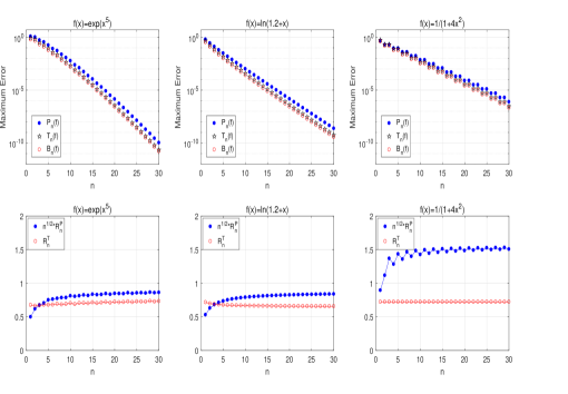
Figure 1: Top row shows the log plot of the maximum error of $\mathcal{B}_{n}(f)$, $\mathcal{T}_{n}(f)$ and $\mathcal{P}_{n}(f)$ for $f(x)=\exp(x^{5})$ (left), $f(x)=\ln(1.2+x)$ (middle) and $f(x)=1/(1+4x^{2})$ (right). Bottom row shows $n^{1/2}\mathcal{R}_{n}^{P}$ and $\mathcal{R}_{n}^{T}$. Here $n$ ranges from 1 to 30.

In Figure 2 we show the maximum error of three approximations as a function of $n$ for the three differentiable functions $f(x)=\exp(-1/x^{2}),(x-\frac{1}{2})_{+}^{3},|\sin(5x)|$ and the corresponding ratios $\mathcal{R}_{n}^{P}$ and $\mathcal{R}_{n}^{T}$. For the first test function, it is infinitely differentiable on $\mathrm{\Omega}$. For the second test function, it is a spline function whose definition is given in (48). Moreover, $f\in C^{2}(\mathrm{\Omega})$ and $f{{}^{\prime\prime\prime}}$ is of bounded variation on $\mathrm{\Omega}$. For the last function, it is absolutely continuous and $f{{}^{\prime}}$ is of bounded variation on $\mathrm{\Omega}$. From the top row of Figure 2 we observe that all three methods $\mathcal{B}_{n}(f)$, $\mathcal{T}_{n}(f)$ and $\mathcal{P}_{n}(f)$ converge at the same rate. From the bottom row of Figure 2 we see that each ratio $\mathcal{R}_{n}^{P}$ and $\mathcal{R}_{n}^{T}$ oscillates around or converges to a finite asymptote as $n\rightarrow\infty$, which implies that $\mathcal{B}_{n}(f)$ is better than $\mathcal{T}_{n}(f)$ and $\mathcal{P}_{n}(f)$ by only some constant factors (for the last two functions, note that $\mathcal{R}_{n}^{P}$ and $\mathcal{R}_{n}^{T}$ approach about $1/2$ as $n\rightarrow\infty$, and thus $\mathcal{B}_{n}(f)$ is better than $\mathcal{T}_{n}(f)$ and $\mathcal{P}_{n}(f)$ by a factor of 2).

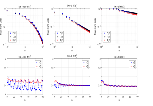
Figure 2: Top row shows the log-log plot of the maximum error of $\mathcal{B}_{n}(f)$, $\mathcal{T}_{n}(f)$ and $\mathcal{P}_{n}(f)$ for $f(x)=\exp(-1/x^{2})$ (left), $f(x)=(x-\frac{1}{2})_{+}^{3}$ (middle) and $f(x)=|\sin(5x)|$ (right). Bottom row shows the corresponding $\mathcal{R}_{n}^{P}$ and $\mathcal{R}_{n}^{T}$. Here $n$ ranges from 1 to 100.

In summary, the above observations suggest the following conclusions:

• For analytic functions, the rate of convergence of $\mathcal{B}_{n}(f)$ is better than that of $\mathcal{T}_{n}(f)$ by some constant factors and is better than that of $\mathcal{P}_{n}(f)$ by a factor of $n^{1/2}$;

• For differentiable functions, however, the rate of convergence of $\mathcal{B}_{n}(f)$ is better than that of $\mathcal{T}_{n}(f)$ and $\mathcal{P}_{n}(f)$ by only some constant factors.

How to explain these observations? Regarding the convergence behavior of $\mathcal{T}_{n}(f)$, sharp bounds for its maximum error have received much attention in recent years. We collect the results in the following.

Theorem 2.1

If $f$ is analytic with $|f(z)|\leq M$ in the region bounded by the ellipse with foci $\pm 1$ and major and minor semiaxis lengths summing to $\rho>1$, then for each $n\geq 0$,

$$\|f-\mathcal{T}_{n}(f)\|_{\infty}\leq\frac{2M}{\rho^{n}(\rho-1)}.$$ (11)

If $f,f{{}^{\prime}},\ldots,f^{(m-1)}$ are absolutely continuous on $\mathrm{\Omega}=[-1,1]$ and $f^{(m)}$ is of bounded variation $V_{m}$ for some integer $m\geq 1$, then for each $n\geq m+1$,

$$\|f-\mathcal{T}_{n}(f)\|_{\infty}\leq\frac{2V_{m}}{\pi m(n-m)^{m}}.$$ (12)

Proof

We refer to (trefethen2013atap, , Chapter 8) for the proof of (11) and (trefethen2013atap, , Chapter 7) for the proof of (12).

A few remarks on Theorem 2.1 are in order.

Remark 1

Notice that these functions $f(x)=\exp(-1/x^{2}),(x-\frac{1}{2})_{+}^{3},|\sin(5x)|$ correspond to $m=\infty$, $m=3$ and $m=1$, respectively. As a consequence, we can deduce from (12) that the rates of convergence of $\mathcal{T}_{n}(f)$ are $O(n^{-k})$ for any $k\in\mathbb{N}$, $O(n^{-3})$ and $O(n^{-1})$, respectively. On the other hand, we can deduce from (timan1963approximation, , Chapter 7) that the rates of convergence of $\mathcal{B}_{n}(f)$ for these three functions are also $O(n^{-k})$ for any $k\in\mathbb{N}$, $O(n^{-3})$ and $O(n^{-1})$, respectively. Clearly, the rates of convergence of $\mathcal{T}_{n}(f)$ and $\mathcal{B}_{n}(f)$ are of the same order, which explain the convergence behavior of $\mathcal{T}_{n}(f)$ observed in Figure 2. For discussions on the comparison of $\mathcal{B}_{n}(f)$ and $\mathcal{T}_{n}(f)$ when $f$ is a polynomial of degree larger than $n$, we refer to clenshaw1964best .

Remark 2

For differentiable functions, the bound (12) is only optimal for functions with interior singularities of integer-order. For functions of fractional smoothness, optimal error estimates of $\mathcal{T}_{n}(f)$ was recently analyzed in liu2019optimal by introducing fractional Sobolev-type spaces and using the fractional calculus properties of Gegenbauer functions of fractional degree. We refer the interested reader to liu2019optimal for more details.

In the following sections, we shall focus on the convergence behavior of the Legendre projection $\mathcal{P}_{n}(f)$ for analytic and several typical kinds of differentiable functions and present some theoretical results concerning its optimal rate of convergence.

3 Optimal rate of convergence of $\mathcal{P}_{n}(f)$ for analytic functions

In this section we study the optimal rate of convergence of $\mathcal{P}_{n}(f)$ for analytic functions. Let $\mathcal{E}_{\rho}$ denote the Bernstein ellipse

$$\mathcal{E}_{\rho}=\left\{z\in\mathbb{C}~{}\bigg{|}~{}z=\frac{u+u^{-1}}{2},~{}~{}|u|=\rho\geq 1\right\},$$ (13)

which has the foci at $\pm 1$ and the major and minor semi-axes are given by $(\rho+\rho^{-1})/2$ and $(\rho-\rho^{-1})/2$, respectively.

Our starting point is the contour integral expression of the Legendre coefficients.

Lemma 1

Suppose that $f$ is analytic in the region bounded by the ellipse $\mathcal{E}_{\rho}$ for some $\rho>1$, then for each $k\geq 0$,

$$a_{k} =\frac{\Gamma(k+1)\Gamma(\frac{1}{2})}{\Gamma(k+\frac{1}{2})i\pi}\oint_{\mathcal{E}_{\rho}}\frac{f(z)}{(z\pm\sqrt{z^{2}-1})^{k+1}}{}_{2}\mathrm{F}_{1}\left[\begin{matrix}k&+1,\frac{1}{2}\\ k+\frac{3}{2}&\end{matrix};\frac{1}{(z\pm\sqrt{z^{2}-1})^{2}}\right]\mathrm{d}z,$$ (14)

where the sign in $z\pm\sqrt{z^{2}-1}$ is chosen so that $|z\pm\sqrt{z^{2}-1}|>1$ and $\Gamma(z)$ is the gamma function. Here ${}_{2}\mathrm{F}_{1}(\cdot)$ is the Gauss hypergeometric function defined by

$${}_{2}\mathrm{F}_{1}\left[\begin{matrix}&a,b\\ c&\end{matrix};z\right]=\sum_{k=0}^{\infty}\frac{(a)_{k}(b)_{k}}{(c)_{k}}\frac{z^{k}}{k!},$$

where $|z|<1$ and $c\neq 0,-1,-2,\ldots$, and $(z)_{k}$ is the Pochhammer symbol defined by $(z)_{0}=1$ and $(z)_{k+1}=(z)_{k}(z+k)$ for $k\geq 0$.

Proof

This contour integral was first derived by Iserles in iserles2011legendre for the purpose of designing some fast algorithms for computing $\{a_{k}\}_{k=0}^{n}$. The idea of his derivation is based on writing $a_{k}$ as a linear combination of $\{f^{(j)}(0)\}$ and then as an integral transform with a Gauss hypergeometric function as its kernel. After that, a hypergeometric transformation was used to replace the original kernel by a new one that converges rapidly, which finally leads to (14). More recently, a new and simpler approach for the derivation of (14) was proposed in wang2016gegenbauer and the idea is simply to rearrange the Chebyshev coefficients of the second kind. We refer the interested reader to iserles2011legendre ; wang2016gegenbauer for more details.

In the following, we state some new upper bounds for the Legendre coefficients, which are simpler but slightly less sharp than the result stated in wang2016gegenbauer . As will be shown later, these new bounds allow us to establish a new and explicit error bound for the Legendre projection $\mathcal{P}_{n}(f)$.

Lemma 2

Suppose that $f$ is analytic in the region bounded by the ellipse $\mathcal{E}_{\rho}$ for some $\rho>1$, then for each $k\geq 0$,

$$|a_{0}|\leq\frac{D(\rho)}{2},\qquad|a_{k}| \leq D(\rho)\frac{k^{1/2}}{\rho^{k}},\quad k\geq 1,$$ (15)

where $D(\rho)$ is defined by

$$D(\rho) =\frac{\displaystyle 2L(\mathcal{E}_{\rho})}{\pi\sqrt{\rho^{2}-1}}\max_{z\in\mathcal{E}_{\rho}}|f(z)|.$$ (16)

Here $L(\mathcal{E}_{\rho})$ denotes the length of the circumference of $\mathcal{E}_{\rho}$.

Proof

From Lemma 1, we immediately obtain

$$|a_{k}| \leq\frac{\Gamma(k+1)\Gamma(\frac{1}{2})}{\Gamma(k+\frac{1}{2})\pi}{}_{2}\mathrm{F}_{1}\left[\begin{matrix}k&+1,\frac{1}{2}\\ k+\frac{3}{2}&\end{matrix};~{}\frac{1}{\rho^{2}}\right]\frac{L(\mathcal{E}_{\rho})}{\rho^{k+1}}\max_{z\in\mathcal{E}_{\rho}}|f(z)|.$$ (17)

Furthermore, for each $k\geq 0$ and $\rho>1$, we have

$${}_{2}\mathrm{F}_{1}\left[\begin{matrix}k&+1,\frac{1}{2}\\ k+\frac{3}{2}&\end{matrix};~{}\frac{1}{\rho^{2}}\right]\leq{}_{2}\mathrm{F}_{1}\left[\begin{matrix}k&+\frac{3}{2},\frac{1}{2}\\ k+\frac{3}{2}&\end{matrix};~{}\frac{1}{\rho^{2}}\right] ={}_{1}\mathrm{F}_{0}\left[\begin{matrix}\frac{1}{2}\\ &\end{matrix};~{}\frac{1}{\rho^{2}}\right]$$

$$=\left(1-\frac{1}{\rho^{2}}\right)^{-1/2}.$$ (18)

Combining (17) and (3), the bound for $|a_{0}|$ follows immediately. We now consider the case $k\geq 1$. To establish an explicit bound for the ratio of gamma functions in (17), we define the following sequence

$$\psi(k)=\frac{\Gamma(k+1)\Gamma(\frac{1}{2})}{\Gamma(k+\frac{1}{2})}k^{-1/2}.$$

It can be easily shown that the sequence $\{\psi(k)\}$ is strictly decreasing. Hence, we obtain

$$\psi(k)\leq\psi(1)=2~{}~{}\Rightarrow~{}~{}\frac{\Gamma(k+1)\Gamma(\frac{1}{2})}{\Gamma(k+\frac{1}{2})}\leq 2k^{1/2}.$$ (19)

Combining (17), (3) and (19) gives the desired result. This completes the proof.

Remark 3

Sharp bounds for the Legendre coefficients of analytic functions were studied in wang2012legendre ; wang2016gegenbauer ; xiang2012error ; zhao2013sharp with different approaches. The new bound (15) is slightly less sharp than the latest result stated in (wang2016gegenbauer, , Corollary 4.5) by a factor of up to $2/\pi^{1/2}$($\approx 1.13$) since we have established a uniform bound for $\psi(k)$ in (19). However, the factor $D(\rho)$ in (16) is independent of $k$, which is more convenient when applying (15) to refine a simple error bound of $\mathcal{P}_{n}(f)$, as will be shown below.

Remark 4

The length of the circumference of $\mathcal{E}_{\rho}$ is given by $L(\mathcal{E}_{\rho})=4E(\varepsilon)/\varepsilon$, where $\varepsilon=2/(\rho+\rho^{-1})$ and $E(z)$ is the complete elliptic integral of the second kind (see, e.g., (olver2010nist, , Equation (19.9.9))). For various approximation formulas of $L(\mathcal{E}_{\rho})$, we refer to the survey article almkvist1988ellipse for an extensive discussion. Moreover, sharp bounds of $L(\mathcal{E}_{\rho})$ are also available (see, e.g., Jameson2014ellipse ), i.e.,

$$L(\mathcal{E}_{\rho})\leq 2\left(\rho+\frac{1}{\rho}\right)+2\left(\frac{\pi}{2}-1\right)\left(\rho-\frac{1}{\rho}\right),\quad\rho\geq 1,$$ (20)

and the above inequality becomes an equality when $\rho=1$ or $\rho\rightarrow\infty$.

With the above Lemma at hand, we are now able to establish an explicit error bound for the Legendre projection $\mathcal{P}_{n}(f)$ in the $L^{\infty}$ norm. Moreover, we show that the derived error bound is optimal up to a constant factor.

Theorem 3.1

Suppose that $f$ is analytic in the region bounded by the ellipse $\mathcal{E}_{\rho}$ for some $\rho>1$. Then, for each $n\geq 0$,

$$\|f-\mathcal{P}_{n}(f)\|_{\infty}\leq\frac{D(\rho)}{\rho^{n}}\left[\frac{(n+1)^{1/2}}{\rho-1}+\frac{(n+1)^{-1/2}}{(\rho-1)^{2}}\right].$$ (21)

Up to a constant factor, the bound on the right hand side is optimal in the sense that it can not be improved in any negative powers of $n$ further.

Proof

As a consequence of Lemma 2, we obtain that

$$\|f-\mathcal{P}_{n}(f)\|_{\infty}\leq\sum_{k=n+1}^{\infty}|a_{k}|\leq D(\rho)\sum_{k=n+1}^{\infty}\frac{k^{1/2}}{\rho^{k}}.$$ (22)

For the last sum in (22), we have

$$\sum_{k=n+1}^{\infty}\frac{k^{1/2}}{\rho^{k}} \leq(n+1)^{-1/2}\sum_{k=n+1}^{\infty}\frac{k}{\rho^{k}}=\frac{1}{\rho^{n}}\left[\frac{(n+1)^{1/2}}{\rho-1}+\frac{(n+1)^{-1/2}}{(\rho-1)^{2}}\right].$$

This proves the bound (21).

We now turn to prove the optimality of the bound (21). By contradiction suppose that it can be further improved in a negative power of $n$, i.e.,

$$\|f-\mathcal{P}_{n}(f)\|_{\infty}\leq n^{-\gamma}\frac{D(\rho)}{\rho^{n}}\left[\frac{(n+1)^{1/2}}{\rho-1}+\frac{(n+1)^{-1/2}}{(\rho-1)^{2}}\right],$$ (23)

where $\gamma>0$. Let us consider a concrete function, e.g., $f(x)=(x-2)^{-1}$. It is easily seen that this function has a simple pole at $x=2$ and therefore $\rho\leq 2+\sqrt{3}-\epsilon$, where $\epsilon>0$ may be taken arbitrary small. On the other hand, using Lemma 1 and the residue theorem, we can write the Legendre coefficients of $f(x)$ as

$$a_{k} =\frac{\Gamma(k+1)\Gamma(\frac{1}{2})}{\Gamma(k+\frac{1}{2})}{}_{2}\mathrm{F}_{1}\left[\begin{matrix}k&+1,\frac{1}{2}\\ k+\frac{3}{2}&\end{matrix};\frac{1}{(2+\sqrt{3})^{2}}\right]\frac{(-2)}{(2+\sqrt{3})^{k+1}}.$$ (24)

Clearly, $a_{k}<0$ for all $k\geq 0$, and it is easy to check that the sequence $\{-a_{k}\}_{k=0}^{\infty}$ is strictly decreasing. Now, we consider the error of the Legendre projection at the point $x=1$. In view of $P_{k}(1)=1$ for $k\geq 0$, we obtain that

$$\left|f(x)-\mathcal{P}_{n}(f)\right|_{x=1} =\sum_{k=n+1}^{\infty}(-a_{k})\geq-a_{n+1}.$$

Thus, combining the above bound with (23) yields

$$-a_{n+1}\leq\|f(x)-\mathcal{P}_{n}(f)\|_{\infty}\leq n^{-\gamma}\frac{D(\rho)}{\rho^{n}}\left[\frac{(n+1)^{1/2}}{\rho-1}+\frac{(n+1)^{-1/2}}{(\rho-1)^{2}}\right].$$ (25)

Furthermore, from (24) we can deduce that the lower bound of $\|f(x)-\mathcal{P}_{n}(f)\|_{\infty}$ behaves like $|a_{n+1}|=O(n^{1/2}(2+\sqrt{3})^{-n})$ and the upper bound of $\|f(x)-\mathcal{P}_{n}(f)\|_{\infty}$ behaves like $O(n^{1/2-\gamma}(2+\sqrt{3}-\epsilon)^{-n})$ as $n\rightarrow\infty$. Clearly, this leads to an obvious contradiction since the upper bound may be smaller than the lower bound when $\epsilon$ is sufficiently small. Therefore, we can conclude that the derived bound (21) is optimal in the sense that it can not be improved in any negative powers of $n$ further. This completes the proof.

Remark 5

From (cheney1998approximation, , p. 131) we know that

$$\frac{\pi}{4}\max_{k\geq n}\left\{|c_{k}|\right\}\leq\|f-\mathcal{B}_{n}(f)\|_{\infty}\leq\sum_{k=n+1}^{\infty}|c_{k}|.$$ (26)

Moreover, from (bernstein1912cheb, , p. 95) we know that $|c_{k}|\leq 2\max_{z\in\mathcal{E}_{\rho}}|f(z)|\rho^{-k}$, and thus the rate of convergence of $\mathcal{B}_{n}(f)$ is $O(\rho^{-n})$ as $n\rightarrow\infty$, i.e., $\|f-\mathcal{B}_{n}(f)\|_{\infty}=O(\rho^{-n})$. Comparing this with (21), it is easy to see that the rate of convergence of $\mathcal{B}_{n}(f)$ is $O(n^{1/2})$ faster than that of $\mathcal{P}_{n}(f)$. Moreover, comparing (21) and (11), we see that the rate of convergence of $\mathcal{T}_{n}(f)$ is also $O(n^{1/2})$ faster than that of $\mathcal{P}_{n}(f)$. These explain the convergence behavior of $\mathcal{P}_{n}(f),\mathcal{T}_{n}(f)$ and $\mathcal{B}_{n}(f)$ illustrated in Figure 1.

4 Optimal rate of convergence of $\mathcal{P}_{n}(f)$ for functions with derivatives of bounded variation

In this section we study optimal rate of convergence of $\mathcal{P}_{n}(f)$ for differentiable functions with derivatives of bounded variation. We start with the case of piecewise analytic functions and then extend our discussion to the case of functions whose $m$th order derivative is of bounded variation. Throughout this paper, we denote by $K$ a generic positive constant independent of $n$.

4.1 Piecewise analytic functions

We first introduce the definition of piecewise analytic function (see, e.g., saff1989poly ).

Definition 1

Let $f$ be a piecewise analytic function, by which we mean there exist a set of points

$$-1<\xi_{1}<\xi_{2}<\cdots<\xi_{\ell}<1,\quad\ell\geq 1,$$

such that the restriction of $f$ to each $[-1,\xi_{1}]$,$[\xi_{1},\xi_{2}]$,$\ldots$,$[\xi_{\ell},1]$ has an analytic continuation to a neighborhood of this closed interval, but $f$ itself is not analytic at each point $\xi_{1},\ldots,\xi_{\ell}$. In the following discussion, we will denote by $\mathrm{PA}(\mathrm{\Omega},\vec{\xi})$, where $\vec{\xi}=(\xi_{1},\ldots,\xi_{\ell})^{T}\in\mathbb{R}^{\ell}$ and $\cdot^{T}$ denotes the transpose, the set of piecewise analytic functions for notational simplicity.

In order to analyze the convergence behavior of $\mathcal{P}_{n}(f)$, we first rewrite it as

$$\mathcal{P}_{n}(f)=\sum_{k=0}^{n}P_{k}(x)\left(k+\frac{1}{2}\right)\int_{-1}^{1}f(y)P_{k}(y)\mathrm{d}y=\int_{-1}^{1}f(y)D_{n}(x,y)\mathrm{d}y,$$ (27)

where $D_{n}(x,y)$ is the Dirichlet kernel of Legendre polynomials defined by

$$D_{n}(x,y) =\sum_{k=0}^{n}\left(k+\frac{1}{2}\right)P_{k}(x)P_{k}(y).$$ (28)

By means of the Christoffel-Darboux identity for Legendre polynomials (shen2011spectral, , p. 51), the Dirichlet kernel can also be written as

$$D_{n}(x,y) =\frac{n+1}{2}\left[\frac{P_{n+1}(x)P_{n}(y)-P_{n+1}(y)P_{n}(x)}{x-y}\right].$$ (29)

In the following we give two useful lemmas.

Lemma 3

For $|x|\leq 1$ and $n\geq 0$, we have

$$|P_{n}(x)|\leq\sqrt{\frac{2}{\pi}}\left(n+\frac{1}{2}\right)^{-1/2}\phi_{n}(x),$$ (30)

where

$$\phi_{n}(x)=\min\left\{(1-x^{2})^{-1/4},\sqrt{\frac{\pi}{2}}\left(n+\frac{1}{2}\right)^{1/2}\right\}.$$ (31)

Proof

Recall the Bernstein-type inequality of Legendre polynomials Antonov1981estimate , i.e.,

$$(1-x^{2})^{1/4}|P_{n}(x)|<\sqrt{\frac{2}{\pi}}\left(n+\frac{1}{2}\right)^{-1/2},\quad x\in[-1,1],$$

and the bound is optimal in the sense that the factor $(n+1/2)^{-1/2}$ can not be improved to $(n+1/2+\epsilon)^{-1/2}$ for any $\epsilon>0$ and the constant $\sqrt{2/\pi}$ is best possible. On the other hand, recall the well known inequality $|P_{n}(x)|\leq 1$. Combining these two inequalities give the desired result.

Lemma 4

Let $|x|\leq 1$ and let $\delta\in(0,1)$.

1. If $|y|\leq 1$, then

   $$|D_{n}(x,y)| \leq\frac{(n+1)^{2}}{2}.$$ (32)

2. If $|y|\leq 1-\delta$, then

   $$|D_{n}(x,y)|\leq Kn,\quad n\gg 1.$$ (33)

Proof

As for (32), it follows from (28) and the inequality $|P_{k}(x)|\leq 1$. As for (33), we split our discussion into two cases: $|x-y|<\delta/2$ or $|x-y|\geq\delta/2$. In the case when $|x-y|<\delta/2$. By (28) and Lemma 3 we obtain that

$$|D_{n}(x,y)|\leq\frac{2}{\pi}\sum_{k=0}^{n}\phi_{k}(x)\phi_{k}(y)\leq\frac{2(n+1)}{\pi}(1-x^{2})^{-1/4}(1-y^{2})^{-1/4}.$$ (34)

For $|y|\leq 1-\delta$, it is easily verified that $|x|\leq 1-\delta/2$, and therefore,

$$|D_{n}(x,y)| \leq\frac{2(n+1)}{\pi}\left(1-\left(1-\frac{\delta}{2}\right)^{2}\right)^{-1/4}(1-(1-\delta)^{2})^{-1/4}$$

$$=\frac{2(n+1)}{\pi}\delta^{-1/2}\left(1-\frac{\delta}{4}\right)^{-1/4}(2-\delta)^{-1/4}$$

$$=O(n).$$ (35)

Next, we consider the case $|x-y|\geq\delta/2$. From (29) and Lemma 3 it follows that

$$|D_{n}(x,y)| \leq\frac{n+1}{\delta}\sqrt{\frac{2}{\pi}}\left(\left(n+\frac{1}{2}\right)^{-1/2}\phi_{n}(y)+\left(n+\frac{3}{2}\right)^{-1/2}\phi_{n+1}(y)\right).$$

$$\leq\frac{2(n+1)}{\delta}\sqrt{\frac{2}{\pi}}\left(n+\frac{1}{2}\right)^{-1/2}(1-y^{2})^{-1/4}$$

$$\leq\frac{2}{\delta^{5/4}}\sqrt{\frac{2}{\pi}}(2-\delta)^{-1/4}(n+1)\left(n+\frac{1}{2}\right)^{-1/2}$$

$$=O(n^{1/2}).$$ (36)

Finally, the desired result (33) follows from (4.1) and (4.1). This completes the proof.

We are now ready to state the first main result of this section.

Theorem 4.1

Assume that $f\in C^{m-1}(\mathrm{\Omega})\cap\mathrm{PA}(\mathrm{\Omega},\vec{\xi})$ for some integer $m\in\mathbb{N}$ and some $\vec{\xi}\in\mathbb{R}^{\ell}$ with $\ell\geq 1$. Then, for $n\gg 1$, we have

$$\|f-\mathcal{P}_{n}(f)\|_{\infty}\leq Kn^{-m}.$$ (37)

Up to constant factors, the bound on the right hand side is optimal in the sense that it is the same as that of $\mathcal{B}_{n}(f)$.

Proof

Since $f\in C^{m-1}(\mathrm{\Omega})$ and is piecewise analytic on $\mathrm{\Omega}$, we know from (saff1989poly, , Theorem 3) that there exists a polynomial $p_{n}$ of degree $n$ such that for all $x\in\mathrm{\Omega}$

$$|f(x)-p_{n}(x)|\leq\frac{C}{n^{m}}e^{-cn^{\alpha}d(x)^{\beta}},$$ (38)

where $\alpha\in(0,1)$ and $\beta\geq\alpha$ or $\alpha=1$ and $\beta>1$, $d(x)=\min_{1\leq k\leq\ell}|x-\xi_{k}|$ and $C,c$ are some positive constants. Taking $\alpha=\beta\in(0,1)$ and recalling that $\mathcal{P}_{n}(f)\equiv f$ whenever $f$ is a polynomial of degree up to $n$, we immediately obtain

$$|f-\mathcal{P}_{n}(f)| \leq|f-p_{n}|+|\mathcal{P}_{n}(f-p_{n})|$$

$$\leq\frac{C}{n^{m}}e^{-c(nd(x))^{\alpha}}+\frac{C}{n^{m}}\int_{-1}^{1}e^{-c(nd(y))^{\alpha}}|D_{n}(x,y)|\mathrm{d}y,$$ (39)

where we have used (38) and (27) in the last step. It remains to show the last integral in (4.1) behaves like $O(1)$ as $n\rightarrow\infty$. For simplicity of presentation, we denote it by $I$. Moreover, we let $I_{1}=[\xi_{1}-\epsilon,\xi_{1}+\epsilon],\ldots,I_{\ell}=[\xi_{\ell}-\epsilon,\xi_{\ell}+\epsilon]$, where $\epsilon>0$ is chosen to be small enough so that these subintervals $I_{1},\ldots,I_{\ell}$ are pairwise disjoint and are contained in the interior of $\mathrm{\Omega}$, i.e., $I_{1},\ldots,I_{\ell}\subset\mathrm{\Omega}$. Then

$$I=\sum_{k=1}^{\ell}\int_{I_{k}}e^{-c(nd(y))^{\alpha}}|D_{n}(x,y)|\mathrm{d}y+\int_{\mathrm{\Omega}\backslash\bigcup_{k=1}^{\ell}I_{k}}e^{-c(nd(y))^{\alpha}}|D_{n}(x,y)|\mathrm{d}y.$$ (40)

For the former sum in (40), notice that $d(y)=|y-\xi_{k}|$ when $y\in I_{k}$, and thus we get

$$\sum_{k=1}^{\ell}\int_{I_{k}}e^{-c(nd(y))^{\alpha}}|D_{n}(x,y)|\mathrm{d}y =\sum_{k=1}^{\ell}\int_{\xi_{k}-\epsilon}^{\xi_{k}+\epsilon}e^{-c(n|y-\xi_{k}|)^{\alpha}}|D_{n}(x,y)|\mathrm{d}y$$

$$=\sum_{k=1}^{\ell}\int_{-\epsilon}^{\epsilon}e^{-c(n|t|)^{\alpha}}|D_{n}(x,t+\xi_{k})|\mathrm{d}t,$$

where we applied the change of variable $y=t+\xi_{k}$ in the last step. Furthermore, using (33) and a change of variable $z=nt$, we obtain

$$\sum_{k=1}^{\ell}\int_{I_{k}}e^{-c(nd(y))^{\alpha}}|D_{n}(x,y)|\mathrm{d}y \leq 2K\ell n\int_{0}^{\epsilon}e^{-c(nt)^{\alpha}}\mathrm{d}t$$

$$\leq 2K\ell\int_{0}^{\infty}e^{-cz^{\alpha}}\mathrm{d}z$$

$$=2K\ell\frac{\Gamma(\alpha^{-1})}{\alpha c^{1/\alpha}}.$$ (41)

For the second term in (40), notice that $d(y)\geq\epsilon$ when $y\in\mathrm{\Omega}\backslash\bigcup_{k=1}^{\ell}I_{k}$, we obtain

$$\int_{\mathrm{\Omega}\backslash\bigcup_{k=1}^{\ell}I_{k}}e^{-c(nd(y))^{\alpha}}|D_{n}(x,y)|\mathrm{d}y \leq e^{-c(n\epsilon)^{\alpha}}\int_{\mathrm{\Omega}\backslash\bigcup_{k=1}^{\ell}I_{k}}|D_{n}(x,y)|\mathrm{d}y$$

$$\leq e^{-c(n\epsilon)^{\alpha}}(n+1)^{2},$$ (42)

where we have used (32) in the last step. Combining (4.1), (4.1) and (4.1) gives the desired result. This completes the proof.

Remark 6

It is clear that the test functions $f(x)=(x-\frac{1}{2})_{+}^{3},|\sin(5x)|$ are piecewise analytic functions on $\mathrm{\Omega}$ and they correspond to $m=3$ and $m=1$, respectively. As a consequence, we can deduce from Theorem 4.1 that the rates of convergence of $\mathcal{P}_{n}(f)$ are $O(n^{-3})$ and $O(n^{-1})$, respectively. Clearly, these rates of convergence are the same order as that of $\mathcal{B}_{n}(f)$ and $\mathcal{T}_{n}(f)$, which explain the convergence behavior of $\mathcal{P}_{n}(f)$ for these two test functions observed in Figure 2.

Remark 7

In Figure 3 we plot the pointwise error of $\mathcal{P}_{n}(f)$ for the function $f(x)=(x-\frac{1}{2})_{+}$. It is clear to see that the maximum error of $\mathcal{P}_{n}(f)$, i.e., $\|f-\mathcal{P}_{n}(f)\|_{\infty}$, is achieved at the singularity of $f$. Moreover, we also observe that the accuracy of $\mathcal{P}_{n}(f)$ is much more accurate than $\mathcal{B}_{n}(f)$ except at the very small neighborhood of the singularity. A similar phenomenon for Chebyshev interpolants has been observed in (trefethen2013atap, , Chapter 16).

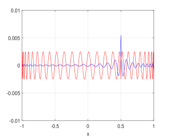
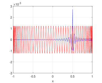
Figure 3: Pointwise error of $\mathcal{P}_{n}(f)$ (blue) and $\mathcal{B}_{n}(f)$ (red) for $n=50$ (left) and $n=100$ (right). Here we choose $f(x)=(x-\frac{1}{2})_{+}$.

4.2 Differentiable functions with derivatives of bounded variation

In this section we consider the case of differentiable functions with derivatives of bounded variation. Specifically, let $m\geq 1$ be an integer and introduce the function space

$$H_{m}=\left\{f~{}|~{}f,f^{\prime},\ldots,f^{(m-1)}\in\mathrm{AC(\Omega)},~{}~{}f^{(m)}\in\mathrm{BV(\Omega)}\right\},$$ (43)

where $\mathrm{AC(\Omega)}$ and $\mathrm{BV(\Omega)}$ denote the space of absolutely continuous functions and the space of bounded variation functions on $\mathrm{\Omega}$, respectively. This space is preferable when developing error estimates for various orthogonal polynomial approximations to differentiable function (see, e.g., liu2019optimal ; trefethen2013atap ; wang2018legendre ; xiang2018jacobi ). For each $f\in\mathrm{PA}(\mathrm{\Omega},\vec{\xi})\cap C^{m-1}(\mathrm{\Omega})$, it is easy to see that the restriction of $f^{(m+1)}$ on each $[-1,\xi_{1}]$,$[\xi_{1},\xi_{2}]$,$\ldots$,$[\xi_{\ell},1]$ is continuous and bounded, and therefore the total variation of $f^{(m)}$ on $\mathrm{\Omega}$ is finite. Hence, we can deduce that $\mathrm{PA}(\mathrm{\Omega},\vec{\xi})\cap C^{m-1}(\mathrm{\Omega})$ is a subset of $H_{m}$. In the following we will extend our analysis to the function space $H_{m}$.

Since $f=\mathcal{P}_{n}(f)$ for $f\in\mathcal{P}_{n}$, using the Peano kernel theorem (brass2011quad, , Section 4.2) we obtain

$$f(x)-\mathcal{P}_{n}(f)=\int_{-1}^{1}f^{(m)}(t)K_{m}(x,t)\mathrm{d}t,$$ (44)

where $K_{m}(x,t)$ is the Peano kernel defined by

$$K_{m}(x,t)=\frac{(x-t)_{+}^{m-1}-\mathcal{P}_{n}((x-t)_{+}^{m-1})}{(m-1)!},$$ (45)

and

$$(x)_{+}^{r}=\left\{\begin{array}[]{ll}0,&\hbox{$x\leq 0$,}\\[8.0pt] x^{r},&\hbox{$x>0$.}\end{array}\right.$$ (48)

We now state some properties of the Peano kernel.

Lemma 5

Let $K_{m}(x,t)$ be the Peano kernel defined in (45). Then for $x\in\mathrm{\Omega}$ and $n\geq m-1$ we have

1. For $m\geq 2$, then $K_{m}(x,\pm 1)=0$. When $m=1$, then $K_{1}(x,1)=0$.

2. For each $m\geq 2$, then $\frac{\mathrm{d}}{\mathrm{d}t}K_{m}(x,t)=-K_{m-1}(x,t).$

3. For $n\geq m$, we have for any $q\in\mathcal{P}_{n-m}$ that $\int_{-1}^{1}q(t)K_{m}(x,t)\mathrm{d}t=0$.

4. For $x,t\in[-1,1]$ and $m\geq 2$, we have $\|K_{m}(x,t)\|_{\infty}\leq Kn^{-m+1}$.

Proof

For the first assertion, notice that $(x-1)_{+}^{m-1}=0$ and $(x+1)_{+}^{m-1}=(x+1)^{m-1}$ when $m\geq 2$. Therefore, $K_{m}(x,\pm 1)=0$. When $m=1$, notice that $(x-1)_{+}^{0}=0$, the desired result follows. For the second assertion, differentiating the Peano kernel with respect to $t$ yields

$$\frac{\mathrm{d}}{\mathrm{d}t}K_{m}(x,t)=-\frac{(x-t)_{+}^{m-2}-\mathcal{P}_{n}((x-t)_{+}^{m-2})}{(m-2)!}=-K_{m-1}(x,t).$$

This proves the second assertion. For the third assertion, we notice that $f\equiv\mathcal{P}_{n}(f)$ whenever $f\in\mathcal{P}_{n}$. Setting $f=q\in\mathcal{P}_{n}$ in (44) gives

$$q-\mathcal{P}_{n}(q) =\int_{-1}^{1}q^{(m)}(t)K_{m}(x,t)\mathrm{d}t=0.$$

Since $q\in\mathcal{P}_{n}$ is arbitrary, this proves the third assertion. For the last assertion, we note that $(x-t)_{+}^{m-1}$ is a piecewise analytic function and $(x-t)_{+}^{m-1}\in C^{m-2}[-1,1]$. The desired result follows from Theorem 4.1. This ends the proof.

We are now ready to state the second main result of this section.

Theorem 4.2

Assume that $f\in H_{m}$ for some integer $m\geq 1$. Then, we have

$$\|f-\mathcal{P}_{n}(f)\|_{\infty}\leq Kn^{-m}.$$ (49)

Proof

Applying the second assertion of Lemma 5 and integrating by parts, we obtain

$$f(x)-\mathcal{P}_{n}(f) =-\int_{-1}^{1}f^{(m)}(t)\frac{\mathrm{d}}{\mathrm{d}t}K_{m+1}(x,t)\mathrm{d}t$$

$$=-\left[f^{(m)}(t)K_{m+1}(x,t)\big{|}_{-1}^{1}-\int_{-1}^{1}K_{m+1}(x,t)\mathrm{d}f^{(m)}(t)\right]$$

$$=\int_{-1}^{1}K_{m+1}(x,t)\mathrm{d}f^{(m)}(t),$$

where the last integral is understood as a Riemann-Stieltjes integral and we have used the first assertion of Lemma 5 in the last step. Furthermore, using the inequality of Riemann-Stieltjes integral, we arrive at

$$\|f(x)-\mathcal{P}_{n}(f)\|_{\infty} \leq\|K_{m+1}(x,t)\|_{\infty}V(f^{(m)}).$$

where $V(f^{(m)})$ is the total variation of $f^{(m)}$. The desired result follows from the last assertion of Lemma 5.

Remark 8

For the test function $f(x)=\exp(-1/x^{2})$, it is infinitely differentiable on $\mathrm{\Omega}$ and $f^{(m)}\in\mathrm{BV(\Omega)}$ for every $m\in\mathbb{N}$. Thus, we can deduce from Theorem 4.2 that the rate of convergence of $\mathcal{P}_{n}(f)$ is $O(n^{-m})$ for any $m\in\mathbb{N}$. Moreover, for the other two test functions $f(x)=(x-\frac{1}{2})_{+}^{3},|\sin(5x)|$, they can also be viewed as differentiable functions with derivatives of bounded variation and they correspond to $m=3$ and $m=1$, respectively. Therefore, we can deduce from Theorem 4.2 that the rate of convergence of $\mathcal{P}_{n}(f)$ is $O(n^{-3})$ and $O(n^{-1})$, respectively. Clearly, these results explain why the rate of convergence of $\mathcal{P}_{n}(f)$ is the same as that of $\mathcal{B}_{n}(f)$ observed in Figure 2.

5 Extension

In this section we extend our discussion to functions of fractional smoothness. We shall restrict our attention to some model functions for the sake of brevity and their results will shed light on the investigation of more complicated functions.

5.1 Functions with an interior singularity of fractional order

Consider the function $f(x)=|x-x_{0}|^{\alpha}$, where $x_{0}\in(-1,1)$ and $\alpha>0$ is not an integer. Clearly, this function has an interior singularity of fractional order. To derive the optimal rate of convergence of $\mathcal{P}_{n}(f)$, we shall combine the asymptotic estimate of the Legendre coefficients of $f$ and the observation in Remark 7.

Using (gradshteyn2007table, , Equation (7.232.3)), we see that

$$a_{k} =\left(k+\frac{1}{2}\right)\int_{-1}^{1}|x_{0}-x|^{\alpha}P_{k}(x)\mathrm{d}x$$

$$=\left(k+\frac{1}{2}\right)\left[\int_{-1}^{x_{0}}(x_{0}-x)^{\alpha}P_{k}(x)\mathrm{d}x+\int_{x_{0}}^{1}(x-x_{0})^{\alpha}P_{k}(x)\mathrm{d}x\right]$$

$$=\left(k+\frac{1}{2}\right)\frac{\Gamma(\alpha+1)\Gamma(k+1)}{\Gamma(k+\alpha+2)}\left[(1-x_{0})^{\alpha+1}P_{k}^{(\alpha+1,-\alpha-1)}(x_{0})\right.$$

$$~{}~{}~{}~{}~{}~{}~{}~{}~{}~{}~{}~{}~{}~{}~{}\left.+(-1)^{k}(1+x_{0})^{\alpha+1}P_{k}^{(\alpha+1,-\alpha-1)}(-x_{0})\right],$$ (50)

where $P_{k}^{(\alpha+1,-\alpha-1)}(x)$ is the Jacobi polynomial of degree $k$. From (szego1975orthogonal, , Theorem 8.21.8) we know that $P_{k}^{(\alpha,\beta)}(x)=O(k^{-1/2})$ where $x\in(-1,1)$ and $\alpha,\beta$ are arbitrary real numbers. Combining this result with the asymptotic behavior of the ratio of gamma functions (olver2010nist, , Equation (5.11.12)), we obtain the estimate $a_{k}=O(k^{-\alpha-1/2})$. On the other hand, as observed in Remark 7, the maximum error of $\mathcal{P}_{n}(f)$ is achieved in a small neighborhood of the singularity $x=x_{0}$. Using the Laplace-Heine formula of the Legendre polynomials (szego1975orthogonal, , Theorem 8.21.1), i.e., $P_{k}(x)=O(k^{-1/2})$ where $x\in(-1,1)$, we see at once that

$$\|f-\mathcal{P}_{n}(f)\|_{\infty}\leq\sum_{k=n+1}^{\infty}|a_{k}||P_{k}(x)|=\sum_{k=n+1}^{\infty}O(k^{-\alpha-1})=O(n^{-\alpha}).$$ (51)

Moreover, this rate of convergence is optimal in the sense that it is the same as that of $\mathcal{B}_{n}(f)$ up to constant factors (see, e.g., (timan1963approximation, , p. 410)). Regarding $\mathcal{T}_{n}(f)$, it has been shown in (liu2019optimal, , Equation (4.61)) that the optimal rate of convergence of $\mathcal{T}_{n}(f)$ is also $O(n^{-\alpha})$. Thus, $\mathcal{T}_{n}(f)$, $\mathcal{B}_{n}(f)$ and $\mathcal{P}_{n}(f)$ have the same rate of convergence for functions with an interior singularity of fractional order.

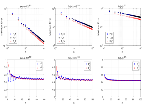
Figure 4: Top row shows the log plot of the maximum error of $\mathcal{B}_{n}(f)$, $\mathcal{T}_{n}(f)$ and $\mathcal{P}_{n}(f)$ for $f(x)=|x-\frac{1}{2}|^{5/2}$ (left), $f(x)=|x-\frac{4}{5}|^{5/4}$ (middle) and $f(x)=|x|^{2/3}$ (right). Bottom row shows the corresponding $\mathcal{R}_{n}^{P}$ and $\mathcal{R}_{n}^{T}$. Here $n$ ranges from 2 to 100.

In Figure 4 we show the maximum error of three methods as a function of $n$ for the three functions $f(x)=|x-\frac{1}{2}|^{5/2},|x-\frac{4}{5}|^{5/4},|x|^{2/3}$ and the corresponding ratios $\mathcal{R}_{n}^{P}$ and $\mathcal{R}_{n}^{T}$. From the top row of Figure 4 we see that all three methods $\mathcal{B}_{n}(f)$, $\mathcal{T}_{n}(f)$ and $\mathcal{P}_{n}(f)$ indeed converge at the same rate. Moreover, the accuracy of $\mathcal{T}_{n}(f)$ and $\mathcal{P}_{n}(f)$ is indistinguishable. From the bottom row of Figure 4 we see that each ratio $\mathcal{R}_{n}^{P}$ and $\mathcal{R}_{n}^{T}$ approaches a constant value as $n\rightarrow\infty$, which confirms that $\mathcal{B}_{n}(f)$ is better than $\mathcal{T}_{n}(f)$ and $\mathcal{P}_{n}(f)$ by only some constant factors (for the three test functions, $\mathcal{R}_{n}^{P},\mathcal{R}_{n}^{T}\in[0.44,0.49]$ as $n\rightarrow\infty$ and thus $\mathcal{B}_{n}(f)$ is better than $\mathcal{T}_{n}(f)$ and $\mathcal{P}_{n}(f)$ by a factor of up to 2.3).

5.2 Functions with endpoint singularities

Consider the functions $f_{\alpha}(x)=(1\pm x)^{\alpha}$, where $\alpha>0$ is not an integer. From (gradshteyn2007table, , Equation (7.311.3)) and setting $\lambda=1/2$, closed forms of the Legendre coefficients are given by

$$a_{k}=(\pm 1)^{k}\frac{2^{\alpha}\Gamma(\alpha+1)^{2}(2k+1)}{\Gamma(\alpha+1-k)\Gamma(\alpha+2+k)},\quad k\geq 0.$$ (52)

Furthermore, combining the reflection formula (olver2010nist, , Equation (5.5.3)) and the asymptotic behavior of the ratio of gamma functions (olver2010nist, , Equation (5.11.12)), we can deduce that

$$a_{k}=(-1)(\mp 1)^{k}\frac{2^{\alpha}\sin(\alpha\pi)\Gamma(\alpha+1)^{2}(2k+1)\Gamma(k-\alpha)}{\pi\Gamma(k+\alpha+2)}=O(k^{-2\alpha-1}).$$

An important observation is that the sequence $\{a_{k}\}_{k>\alpha}$ has the same constant sign when $f_{\alpha}(x)=(1-x)^{\alpha}$ and has alternating signs when $f_{\alpha}(x)=(1+x)^{\alpha}$. Recall $P_{k}(\pm 1)=(\pm 1)^{k}$, we can deduce that the maximum error of $\mathcal{P}_{n}(f_{\alpha})$ is taken at $x=1$ for $f_{\alpha}(x)=(1-x)^{\alpha}$ and at $x=-1$ for $f_{\alpha}(x)=(1+x)^{\alpha}$. Therefore, we obtain for $n\geq\lfloor\alpha\rfloor$ that

$$\|f_{\alpha}-\mathcal{P}_{n}(f_{\alpha})\|_{\infty}=\sum_{k=n+1}^{\infty}|a_{k}|=O(n^{-2\alpha}).$$ (53)

We remark that this result is optimal since the rate of convergence of $\mathcal{B}_{n}(f_{\alpha})$ is $O(n^{-2\alpha})$ (see, e.g., (timan1963approximation, , p. 411)). Moreover, from liu2019optimal we know that the rate of convergence of $\mathcal{T}_{n}(f)$ is also $O(n^{-2\alpha})$. Thus, these three approaches $\mathcal{B}_{n}(f_{\alpha})$, $\mathcal{P}_{n}(f_{\alpha})$ and $\mathcal{T}_{n}(f_{\alpha})$ converge at the same rate.

In Figure 5 we show the maximum error of $\mathcal{B}_{n}(f)$, $\mathcal{T}_{n}(f)$ and $\mathcal{P}_{n}(f)$ as a function of $n$ for the three functions $f(x)=(1+x)^{5/2},(1-x^{2})^{3/2},\cos^{-1}(x)$ and the corresponding ratios $\mathcal{R}_{n}^{P}$ and $\mathcal{R}_{n}^{T}$. From the top row of Figure 5 we see that all three methods indeed converge at the same rate. From the bottom row of Figure 5 we see that each ratio $\mathcal{R}_{n}^{P}$ and $\mathcal{R}_{n}^{T}$ converges to a finite asymptote as $n\rightarrow\infty$, which means that $\mathcal{B}_{n}(f)$ is better than $\mathcal{T}_{n}(f)$ and $\mathcal{P}_{n}(f)$ by only some constant factors (for these three test functions, $\mathcal{R}_{n}^{P}\in[0.17,0.29]$ and $\mathcal{R}_{n}^{T}\in[0.44,0.49]$ as $n\rightarrow\infty$ and thus $\mathcal{B}_{n}(f)$ is better than $\mathcal{P}_{n}(f)$ by at most a factor of $5.9$ and is better than $\mathcal{T}_{n}(f)$ by at most a factor of 2.3).

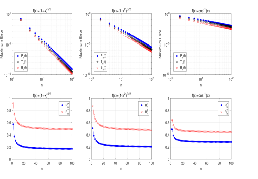
Figure 5: Top row shows the log plot of the maximum error of $\mathcal{B}_{n}(f)$, $\mathcal{T}_{n}(f)$ and $\mathcal{P}_{n}(f)$ for $f(x)=(1+x)^{5/2}$ (left), $f(x)=(1-x^{2})^{3/2}$ (middle) and $f(x)=\cos^{-1}(x)$ (right). Bottom row shows the corresponding $\mathcal{R}_{n}^{P}$ and $\mathcal{R}_{n}^{T}$. Here $n$ ranges from 2 to 100.

Remark 9

For $f_{\alpha}(x)$, it has been shown in (wang2016gegenbauer, , Theorem 5.10) that

$$\frac{a_{k}}{c_{k}}=\frac{\Gamma(\alpha+1)}{\Gamma(\alpha+\frac{1}{2})}\pi^{1/2}+O(k^{-1}).$$ (54)

It is easy to verify that the first term on the right hand side is always greater than one for $\alpha>0$ and is strictly increasing as $\alpha$ grows. Moreover, similar to the Legendre case, we can show that the maximum error of $\mathcal{T}_{n}(f)$ is also achieved at $x=\mp 1$ for $f_{\alpha}(x)=(1\pm x)^{\alpha}$, i.e., $\|f_{\alpha}-\mathcal{T}_{n}(f_{\alpha})\|_{\infty}=\sum_{k=n+1}^{\infty}|c_{k}|$. Combining this with (53) and (54), we can deduce that $\mathcal{T}_{n}(f_{\alpha})$ is better than $\mathcal{P}_{n}(f_{\alpha})$ by a constant factor of $\frac{\Gamma(\alpha+1)}{\Gamma(\alpha+\frac{1}{2})}\pi^{1/2}$ as $n\rightarrow\infty$. This means that the larger $\alpha$, the better the accuracy of $\mathcal{T}_{n}(f_{\alpha})$ than $\mathcal{P}_{n}(f_{\alpha})$, and this phenomenon can be seen clearly from the bottom row of Figure 5.

6 Concluding remarks

In this paper we have studied the optimal rate of convergence of Legendre projections $\mathcal{P}_{n}(f)$ in the $L^{\infty}$ norm for analytic and differentiable functions. For analytic functions, we showed that the optimal rate of convergence of $\mathcal{B}_{n}(f)$ is faster than that of $\mathcal{P}_{n}(f)$ by a factor of $n^{1/2}$. For differentiable functions such as piecewise analytic functions and functions of fractional smoothness, however, we improved the existing results and showed that the rate of convergence of $\mathcal{B}_{n}(f)$ is better than that of $\mathcal{P}_{n}(f)$ by only some constant factors (the factor is between $2$ to $6$ for most of examples displayed in this paper). Our results provide new insights into the approximation power of $\mathcal{P}_{n}(f)$.

Finally, we present some problems for future research:

• In Figure 3, we have illustrated the pointwise error of $\mathcal{P}_{n}(f)$. It can be seen that $\mathcal{P}_{n}(f)$ converges actually much faster than $\mathcal{B}_{n}(f)$ when $x$ is far from the singularity of $f$. It would be interesting to establish a precise estimate on the rate of pointwise convergence of $\mathcal{P}_{n}(f)$ to explain this observation.

• Gegenbauer and Jacobi projections are widely used in spectral methods for differential and integral equations and their optimal error estimates are often required in these applications. Our work can be extended to these two cases (see wang2020gegenbauer for the case of Gegenbauer projections). Following the same line of Theorem 4.1, it is possible to establish an optimal error estimate of Jacobi projections for piecewise analytic functions by combining the result (saff1989poly, , Theorem 3) and some sharp estimates of the Dirichlet kernel of Jacobi polynomials. Moreover, for functions of fractional smoothness, it is also possible to establish some optimal error estimates of Jacobi projections by combining the observation in Remark 7 and sharp estimates of Jacobi expansion coefficients (see xiang2018jacobi ).

• Spectral interpolation, i.e., polynomial interpolation in roots or extrema of Legendre, and, more generally, Gegenbauer and Jacobi polynomials, is a powerful approach for approximating smooth functions that are difficult to compute and serves as theoretical basis for spectral collocation methods (see, e.g., (shen2011spectral, , Chapter 3)). It is of interest to study the comparison of the convergence behavior of spectral interpolation and that of the best approximation $\mathcal{B}_{n}(f)$ for analytic and differentiable functions.

- (1) G. Almkvist and B. Berndt, Gauss, Landen, Ramanujan, the arithmetic-geometric mean, ellipses, , and the ladies diary, Amer. Math. Monthly, 95(7):585-608, 1988.
- (2) B. K. Alpert and V. Rokhlin, A fast algorithm for the evaluation of Legendre expansions, SIAM J. Sci. Statist. Comput., 12(1):158-179, 1991.
- (3) V. A. Antonov and K. V. Holsevnikov, An estimate of the remainder in the expansion of the generating function for the Legendre polynomials (Generalization and improvement of Bernstein’s inequality), Vestnik Leningrad University Mathematics, 13, 163–166, 1981.
- (4) S. Bernstein, Sur l’ordre de la meilleure approximation des fonctions continues par les polynômes de degré donné, Mem. Cl. Sci. Acad. Roy. Belg. 4:1-103, 1912.
- (5) H. Brass and K. Petras, Quadrature Theory: The Theory of Numerical Integration on a Compact Interval, Amer. Math. Soc., Providence, Rhode Island, 2011.
- (6) C. Canuto, M. Y. Hussaini, A. Quarteroni and T. A. Zang, Spectral Methods: Fundamentals in Single Domains, Springer, 2006.
- (7) E. W. Cheney, Introduction to Approximation Theory, AMS Chelsea Publishing, Providence, RI, 1998.
- (8) C. W. Clenshaw, A comparison of “best” polynomial approximations with truncated Chebyshev series expansions, SIAM Numer. Anal., 1(1):26-37, 1964.
- (9) P. J. Davis and P. Rabinowitz, Methods of Numerical Integration, Second edition, Academic Press, London, 1984.
- (10) T. A. Driscoll, H. Hale and L. N. Trefethen, Chebfun User’s Guide, Pafnuty Publications, Oxford, 2014.
- (11) K. Eriksson, Some error estimates for the -version of the finite element method, SIAM J. Numer. Anal., 23(2): 403-411, 1986.
- (12) I. S. Gradshteyn and I. M. Ryzhik, Table of Integrals, Series, and Products, Seventh Edition, Academic Press, 2007.
- (13) W. Gui and I. Babuška, The and - versions of the finite element method in 1 dimension, Numer. Math., 49:577-612, 1986.
- (14) J. H. Hesthaven, S. Gottlieb and D. Gottlieb, Spectral Methods for Time-Dependent Problems, Cambridge University Press, 2007.
- (15) A. Iserles, A fast and simple algorithm for the computation of Legendre coefficients, Numer. Math., 117(3):529-553, 2011.
- (16) G. J. O. Jameson, Inequalities for the perimeter of an ellipse, Math. Gazette, 98:227-234, 2014.
- (17) W.-J. Liu, L.-L. Wang and H.-Y. Li, Optimal error estimates for Chebyshev approximation of functions with limited regularity in fractional Sobolev-type spaces, Math. Comp., 88(320):2857–2895, 2019.
- (18) J. C. Mason and D. C. Handscomb, Chebyshev Polynomials, Chapman and Hall/CRC, Boca Raton, 2003.
- (19) C. K. Qu and R. Wong, Szego’s conjecture on Lebesgue constants for Legendre series, Pacific J. Math., 135(1):157-188, 1988.
- (20) F. W. J. Olver, D. W. Lozier, R. F. Boisvert and C. W. Clark, NIST Handbook of Mathematical Functions, Cambridge University Press, 2010.
- (21) A. Osipov, V. Rokhlin and H. Xiao, Prolate Spheroidal Wave Functions of Order Zero: Mathematical Tools for Bandlimited Approximation, Springer, 2013.
- (22) T. J. Rivlin, An introduction to the approximation of functions, Dover Publications, Inc. New York, 1981.
- (23) E. B. Saff and V. Totik, Polynomial approximation of piecewise analytic functions, J. London Math. Soc., s2-39:487-498, 1989.
- (24) J. Shen, Efficient spectral-Galerkin method I. Direct solvers of second-and fourth-order equations using Legendre polynomials, SIAM J. Sci. Comput., 15(6):1489-1505, 1994.
- (25) J. Shen, T. Tang and L.-L. Wang, Spectral Methods: Algorithms, Analysis and Applications, Springer, Heidelberg, 2011.
- (26) P. K. Suetin, Representation of continuous and differentiable functions by Fourier series of Legendre polynomials, Dokl. Akad. Nauk SSSR, 158(6):1275-1277, 1964.
- (27) G. Szegő, Orthogonal Polynomials, volume 23, American Mathematical Society, 1939.
- (28) A. F. Timan, Theory of Approximation of Functions of a Real Variable, Pergamon Press, Oxford, 1963.
- (29) A. Townsend, M. Webb and S. Olver, Fast polynomial transforms based on Toeplitz and Hankel matrices, Math. Comp., 87(312):1913-1934, 2018.
- (30) L. N. Trefethen, Approximation Theory and Approximation Practice, SIAM, 2013.
- (31) H.-Y. Wang and S.-H. Xiang, On the convergence rates of Legendre approximation, Math. Comp., 81(278):861–877, 2012.
- (32) H.-Y. Wang, On the optimal estimates and comparison of Gegenbauer expansion coefficients, SIAM J. Numer. Anal., 54(3):1557-1581, 2016.
- (33) H.-Y. Wang, A new and sharper bound for Legendre expansion of differentiable functions, Appl. Math. Letters, 85:95-102, 2018.
- (34) H.-Y. Wang, On the optimal rates of convergence of Gegenbauer projections, arXiv:2008.00584, 2020.
- (35) S.-H. Xiang, On error bounds for orthogonal polynomial expansions and Gauss-type quadrature, SIAM J. Numer. Anal., 50(3):1240–1263, 2012.
- (36) S.-H. Xiang and G.-D. Liu, Optimal decay rates on the asymptotics of orthogonal polynomial expansions for functions of limited regularities, Numer. Math., 145:117-148, 2020.
- (37) X.-D. Zhao, L.-L. Wang and Z.-Q. Xie, Sharp error bounds for Jacobi expansions and Gegenbauer-Gauss quadrature of analytic functions, SIAM J. Numer. Anal., 51(3):1443-1469, 2013.