Electrical transport properties of bulk tetragonal CuMnAs
Abstract
Temperature-dependent resistivity and magnetoresistance are measured in bulk tetragonal phase of antiferromagnetic CuMnAs and the latter is found to be anisotropic both due to structure and magnetic order. We compare these findings to model calculations with chemical disorder and finite-temperature phenomena included. The finite-temperature ab initio calculations are based on the alloy analogy model implemented within the coherent potential approximation and the results are in fair agreement with experimental data. Regarding the anisotropic magnetoresistance (AMR) which reaches a modest magnitude of 0.12%, we phenomenologically employ the Stoner-Wohlfarth model to identify temperature-dependent magnetic anisotropy of our samples and conclude that the field-dependence of AMR is more similar to that of antiferromagnets than ferromagnets, suggesting that the origin of AMR is not related to isolated Mn magnetic moments.
pacs:
laterThe emergent field of antiferromagnetic (AFM) spintronicsBaltz:2018_a has brought one particular AFM metal to prominence: CuMnAs. Apart from electrical switchingKaspar:2019_a and domain wall manipulationWadley:2018_a the main focus in exploring its response to electric field has so far been on the optical range (ellipsometry and photoemission spectroscopy used to validate band structure calculationsVeis:2018_a ) and also on the staggered spin polarisation induced by electric field.Zelezny:2014_a The latter led to the discovery of an efficient means to manipulateWadley:2016_a magnetic moments in an AFM and this, in turn, allowed the construction of memory prototypes operating at room temperatureOlejnik:2017_a where information is stored in the direction of magnetic moments. As a method for read-out, anisotropic magnetoresistance (AMR) is used and the primary aim of this work is to explore this very phenomenon in CuMnAs. Contrary to previous recent studies of CuMnAs which entailed epitaxially grown thin layers,Wadley:2013_a we now focus on bulk material.
In the bulk form, CuMnAs was originally reported to have orthorhombic structureMundelein:1992_a while thin films grown on GaP or GaAs substratesKrizek:2019_a adopt a tetragonal phase. Recent studies of off-stoichiometric Cu1+xMn1-xAs compoundsUhlirova:2015_a have shownEmmanoulidou:2017_a ; Uhlirova2019 that their crystal structure is rather sensitive to the composition. While the stoichiometric CuMnAs compounds crystallise in an orthorhombic structure (Pnma), few percent of copper excess at the expense of Mn turns the structure to a tetragonal one (P4/nmm). In the tetragonal phase, the Néel temperature reaches 507 K for Cu1.02Mn0.99As and decreases with decreasing Mn content rather moderately; samples with more off-stoichiometric composition have lower Néel temperatures, for example K forUhlirova2019 . Our focus, however, will be on the nearly-stoichiometric tetragonal systems.
The following section describes the fabrication of samples for electrical transport measurements from a single-crystalline grain and acquired experimental data. Modelling and interepretative approaches are introduced in Sec. II and sections III and IV are devoted to models of zero-field transport and AMR, respectively. The two appendices focus on magnetic anisotropy of CuMnAs and its modelling and certain specialised aspects of microscopic transport calculations.
I Experimental
I.1 Growth and preparation
A sample of tetragonal CuMnAs was prepared by reaction of high purity copper, manganese and arsenic as previously reported.Uhlirova2019 Tetragonal P4/nmm structure was confirmed by powder x-ray diffraction at room temperature on Bruker D8 Advance diffractometer.Uhlirova2019 Composition analysis performed by energy-dispersive x-ray detector (EDX) suggests a slight prevalence of copper, the stoichiometry being 1.02(1):0.99(2):0.99(2) for Cu:Mn:As; Néel temperature () is 507 K. From thus obtained polycrystal, a single-crystal grain was cleaved, oriented using x-ray diffraction and its orientation was further refined on an SEM stub holder using electron backscatter diffaction (EBSD).
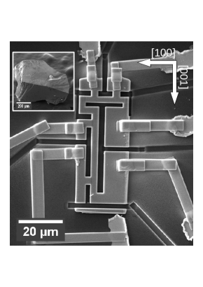
For transport measurements, we adopted the sample fabrication introduced by Moll et al.Moll2015 ; Moll2016 ; Moll2016:CdAs A rectangular lamella extending in the -directions of dimensions 60 was isolated out of a single-crystal grain using 30 kV Ga2+ Focused Ion Beam (FIB) Tescan Lyra XMH and transported to sapphire chip with contact pads (5 nm Cr + 150 nm Au) prepared by photolithography. The lamella was microstructured into a shape presented in Fig. 1 and it was conductively bonded to the contact pads using FIB assisted chemical vapor deposition of Pt. Typical resistance of each contact prepared by this method was around 50 . To improve the contact resistance, we further sputtered the sample with a 100 nm Au layer and removed the excess gold from the top of our sample and in between the contacts using the FIB. This resulted in an order of magnitude lower resistance of 5 per contact.
This method allows us to precisely control the orientation of the sample, which is essential due to highly anisotropic behaviour of CuMnAs which we demonstrate in the following. Furthermore, structuring the sample into a long thin bar allows us to obtain a high signal-to-noise ratio without using high current and thus avoiding self heating at low temperatures.
Resistivity measurement in a temperature range from 2 to 400 K was carried out using a Quantum Design Physical Property Measurement System with a Horizontal Rotator option. Typical currents were of the order of 100 A which translates into current densities ranging from to Am-2 (small compared to what is used in CuMnAs-based memory devices as writing pulsesKaspar:2019_a ). The error in calculating geometrical factor of the bulk device presented here is about 15 %. This translates into a substantial part of error in determining the bulk resistivity.
I.2 Transport measurements
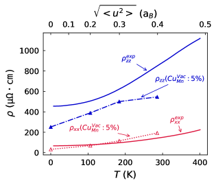
Transport properties of tetragonal CuMnAs have previously been explored only in thin films.Wadley:2013_a Since all epitaxial growth processes reported so far occur in the direction, only in-plane resistivity ( or -axis direction) can be found in literature. Contrary to the thin films, our bulk devices allow for both and the out-of-plane component to be measured (here, we refer to crystallographic directions; both and are measured in the plane of the lamella). In-plane data in Fig. 2 are similar to previously published resultsWadley:2013_a and we take notice of the large structural anisotropy, i.e. resistivity along the -axis being almost an order of magnitude larger (at low temperatures, the ratio to in-plane resistivity is and it slightly decreases at higher temperature). Given the layered structure of CuMnAs, this fact is perhaps not very surprising. Low-temperature cm is somewhat lower (about 20%) than for thin layers of Ref. Wadley:2013_a, . This may be due to slightly different composition of the compared materials or sample quality; the residual resitivity ratios (RRRs) of bulk and thin films samples are 2.2 and 1.8, respectively, and more recent samplesKrizek:2019_a reach an even higher RRR of 3. An example of model calculations in Fig. 2 is further discussed below (see Sec. III): for now, the data points (triangles) should only demonstrate the typical level of agreement with one specific sort of impurities consistent with the known chemical composition of the studied samples. We stress that a significantly better level of agreement is achievable but only at the cost of less realistic model parameters (such as impurity concentration).
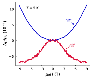
When a magnetic field is switched on, we find a very different response for in-plane and out-of-plane directions: the former shows a negative magnetoresistance — common in magnetic materials when an applied field suppresses spin fluctuations — but increases, see Fig. 3. In both cases, the magnetic field is perpendicular to the current direction, i.e. along [010]. Apart from the AMR effect, the negative magnetoresistance could be related to some kind of magnetic moment response to the applied magnetic field (it is prominent at lower ) while the usual positive magnetoresistance in metals dominates at larger magnetic fields. For current along the -axis, the manipulation of magnetic moments is of no effect (they always remain perpendicular to the current direction) and only the positive magnetoresistance remains.
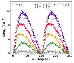
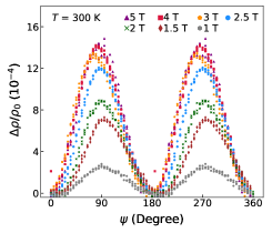
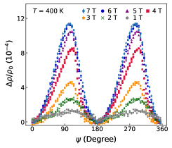
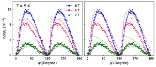
Focusing on in-plane magnetotransport, we also find a clear anisotropy (i.e. different from when ).note1 Here, it should be noted that large magnetic anisotropies force the Néel vector into the -plane (see Appendix A) and conceivably, there remain weak in-plane anisotropies which allow for the magnetic moments to be moved within the plane easily. Angular sweeps shown in Fig. 4 suggest both the presence of AMR and temperature-dependent magnetic anisotropies which we discuss in Sec. IV. We observe a gradual increase of the AMR amplitude up to T and above this magnetic field, the AMR signal does not change (measured up to 9 T, not shown). Low temperature ( K) and close-to-Néel-temperature ( K ) measurements show clearly different distorsion of the signal, see also Eq. (3). Such cosine-squared form would be typical of polycrystalline samplesRushforth:2007_a if magnetocrystalline anisotropy were negligible ( is the angle between and the current direction, see Fig. 1).
 |
 |
 |
 |
II Introduction to modelling
We employ two approaches to interpret our measured data: a microscopic model of electric transport where the direction of magnetic moments present in the system is assumed to be known; and a phenomenological one based on a Stoner-Wohlfarth model where the coupling between external magnetic field and magnetic order of CuMnAs samples is investigated. The latter approach allows to partially overcome our lack of knowledge about the precise nature of potential magnetic impurities. It serves the purpose of interpreting angular sweeps in Fig. 4 where the externally controlled parameter is rather than directly the magnetic moments.
Our microscopic modelling is based on the tight-binding linear muffin-tin orbital (TB-LMTO) method with the atomic sphere approximation and the multicomponent coherent potential approximation (CPA) IT-book . Calculations employ the Vosko-Wilk-Nusair exchange-correlation potentialVosko1980 and Hubbard was used in the fully relativistic LSDA+ scheme for -orbitals of Mn, similarly to Refs. DW2019-JMMM, (TB-LMTO) and Veis:2018_a, (LAPW). The value Ry quoted in Tab. 1 was found consistent with optical and photoemission spectra in the latter reference. The scalar-relativistic methods (see Tab. 5 in Appendix B) are used only for a comparison with previous results.Maca:2017_a ; Maca2019 Band structures yielded by different approaches (including ) can be found in Ref. DW2019-JMMM, .
Electrical transport properties are studied in a framework of the linear response theory and the Kubo-Bastin formula,Turek:2012_a the velocity operators describe intersite hoppingsIT-transport and we take into account CPA-vertex corrections.KC-multilayers Longitudinal conductivities are given only by the Fermi-surface term; therefore, the Fermi-sea contribution IT-FermiSea is omitted. Finite-temperature atomic displacements (phonons) are treated by alloy analogy model (AAM)Ebert2015 ; Kodderitzsch2013 ; Glasbrenner2014 ; Starikov2018 ; this model has recently been incorporated into the TB-LMTO-CPA technique.
For the inclusion of phonons, an extended spdf-basis is needed because of transformations of the LMTO potential functions.DW2017-IEEE ; DW2017-SPIE To compare novel results with literature,Maca:2017_a ; Maca2019 a few spd-calculations are shown in Appendix (Tab. 5). Fluctuations of magnetic moments at nonzero temperatures are included by the tilting modelDW-newJMMM which was shown to describe low-temperature electrical transport of CuMnAs well.DW2019-JMMM Fluctuations of magnetic moments at nonzero temperatures are included only by the disordered local moment (DLM) approach.Kudrnovsky:2012_a Tilting of magnetic moments from their equilibrium direction could be also included within the AAMStarikov2018 as well as our TB-LMTO AAMDW2019-JMMM , but it is beyond the scope of this study. Zero-temperature calculations that involve magnetic impurities (such as Mn atom substituting Cu or As) are also based on the DLM approach. With this machinery at hand, temperature-dependent resistivity can successfully be modelled, provided we specify the source of scattering at (otherwise, at low temperatures).
| Formation | Resistivity [cm] | ||||
|---|---|---|---|---|---|
| energy | |||||
| Defect | [eV] Maca2019 | ||||
| Vac | 31 | 184 | 20 | 181 | |
| Vac | 16 | 79 | 11 | 92 | |
| Mn | 112 | 263 | 150 | 915 | |
| Cu | 0.34 | 23 | 131 | 8 | 57 |
| Cu | 1.15 | 121 | 481 | 163 | 1299 |
| As | 1.73 | 114 | 359 | 123 | 694 |
| As | 1.79 | 141 | 476 | 161 | 617 |
| Mn | 1.92 | 147 | 423 | 186 | 1784 |
| Vac | 2.18 | 210 | 306 | 284 | 1556 |
| CuMn | - | 120 | 393 | 142 | 882 |
III Ab initio transport at zero field
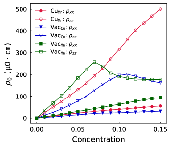
We first focus on residual resistivity. Experimentally, we know that stoichiometry of our CuMnAs samples is 1:1:1 within a few per cent margin and that puts a limit of maximum impurity concentration. Tab. 1 gives an overview of calculated resistivities for various types of impurities (5% of the respective impurity). It should be pointed out that fundamentally different sources of scattering than those listed in Tab. 1 may occur (even at zero temperature), e.g. structural defects such as linear dislocations have recentlyKrizek:2019_a been identified in epitaxial layers.
With this provision, the following conclusions can be drawn regarding resistivities in the absence of external magnetic field. (i) In a very broad picture, all of the listed values of resistivities are plausible; note that exact concentration of impurities is not known for our samples so even large values of seen in Tab. 1 could be compatible with experimental data in Fig. 2 supposing the given type of impurity occurs at a low concentration. (ii) All listed cases involve a clear structural anisotropy . These two basic observations do not principially exclude any of the options in the table, however, (iii) defects involving arsenic, both as a dopant or as a site to be occupied by another atom (substitutional or interstitial positions), seem unlikely given prohibitive formation energies.Maca2019 (iv) Among the five remaining options, those compatible with Cu-rich stoichiometry show resistivity somewhat low compared to experimental data. (v) At this point (i.e. based on calculations in Tab. 1), the most likely scenario, disregarding additional sources of scattering,Krizek:2019_a would thus entail a combination of at least two types of impurities: for example Cu substituting Mn (CuMn) and a Cu/Mn swap (CuMn), both at concentrations of few per cent.
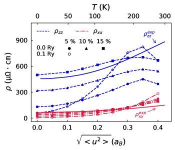
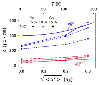
Next, we consider the temperature dependence of resistivity and here, the primary source of scattering are the phonons. As a note of caution, we remark that calculated results are plotted as a function of and conversionDW2019-PRB into requires the knowledge of Debye temperature . (We use the value from orthorhombic phase, see Ref. DW2019-JMMM, for explanation.) Calculations with 5% of CuMn and in Fig. 5 show a reasonable trend but overall values (in particular, of ) are too low. Combination with other types of impurities such asnote3 Cu offers a partial remedy (see model data in Fig. 2) but since concentration-dependence of resistivity is not always linear (see Appendix B and Fig. 9), construction of a quantitative model is difficult. We note that decreasing resistivity for high magnitudes of atomic displacements (see Fig. 5) is probably caused by an increase of DOS at the Fermi level, similarly the effect of magnons and phonons.DW2019-JMMM The same effect may be responsible for nonmonotonic dependence of resistivity on concentration of Cu: both observations clearly contradict the Matthiessen rule and are further discussed in Appendix B.
With temperature–dependent resistivity, phonons are not the sole source of scattering to be considered; rather, combined effect of impurities, phonons, and magnons should be taken into account. Above, we have shown a deviation of the resistivity from Matthiessen’s rule for impurities and phonons; in Ref. DW2019-JMMM, , the same was reported for phonons and magnons. In that reference, we numerically justified a collinear uncompensated disordered local moment (uDLM) model of spin fluctuations and we demonstrated, that the tilting model of the magnetic disorder agrees well with experimental data up to room temperature. We now adopt the second approach and illustrate the combined effect of phonons and magnons and static CuMn impurities. A similar model was discussed in Ref. Kelly2018, (relativistic effects in this context can also be consideredtwoRefsDavid ). A decrease of mean local magnetic moment of Mn atoms was mapped on Monte-Carlo simulationsMaca2019 to obtain the temperature dependence of the spin fluctuations.DW2019-JMMM ; DW2019-PRB Data presented in Tab. 2 show that even for lower concentration of CuMn, the combined effect of phonon and magnon scattering close to the room temperature leads to clearly exceeding the experimental values while remains underestimated.
| CuMn: 5 % | CuMn: 10 % | ||||
| Effects | |||||
| 0 | - | 23 | 131 | 41 | 319 |
| Ph. | 39 | 190 | 55 | 371 | |
| 65 | Mag. | 40 | 215 | 55 | 428 |
| P.+M. | 59 | 269 | 72 | 474 | |
| Ph. | 172 | 450 | 161 | 566 | |
| 230 | Mag. | 115 | 474 | 110 | 724 |
| P.+M. | 257 | 345 | 263 | 450 |
The underestimated values of structural anisotropy seem to be a general feature of our calculations. Previous calculations were obtained without (except for one dataset in Fig. 5 which we wish to discuss now); however, the electronic structure has not yet been reliably determined and the LSDA+ agrees the best with calculationsDW2019-JMMM when Ry. We emphasize, that the band strucutre pertains to CuMnAs without any disorder, while the transport is studied in disordered samples. Therefore, we consider the band strucutre to be of lesser importance for explaining the electrical transport than the DOS. The temperature-dependent resistivity already for Ry increases about twice faster than both measured data and Ry calculations; see Fig. 5 for CuMn. We have investigated also the role of on other impurities and finite-temperature disorder (not shown here) and, in general, nonzero Hubbard parameter makes both increase and decrease of the resistivity more significant (compared to vanishing). This can be attributed to decreasing DOSDW2019-JMMM around for increasing and, therefore, a larger sensitivity of electrical transport on small changes (caused by impurities or finite-temperature disorder).
IV AMR Modelling
Experimental data (angular sweeps in Fig. 4) show a pronounced AMR with two-fold symmetry reaching at saturation (here, is the planar average of resistivity). Theoretical data, see Tab. 3, suggest that this magnitude of AMR is compatible with basically any type of static disorder considered so far. Larger theoretical values (compared to the measured ones), however, indicate that it is not the whole system that responds to the applied magnetic field : for example, magnetic anisotropy for a large part of magnetic moments would not be overcome by available in our experiments and only few free moments would move. (Such free moments could be related to structural defects.) In the case of Cu/Mn swaps, the difference is extreme so either this defect is not very common in our samples or it is largely insensitive to .
| Fully rel., spd | Fully rel., spdf | ||||
|---|---|---|---|---|---|
| Defect | |||||
| Vac | 6.09 | 1.16 | -2.08 | 2.01 | |
| Vac | -1.04 | 1.08 | 5.24 | -1.85 | |
| Mn | 2.52 | 6.25 | 2.29 | 1.59 | |
| Cu | 6.69 | -5.32 | -2.05 | 1.34 | |
| Cu | 1.70 | 1.03 | 1.66 | 1.80 | |
| As | 2.79 | 1.05 | 2.42 | 1.13 | |
| As | 3.41 | 1.31 | 1.60 | 1.30 | |
| Mn | 2.95 | 1.20 | 2.47 | 9.98 | |
| Vac | 2.17 | 1.87 | 2.99 | 2.27 | |
| CuMn | 2.54 | 2.03 | 2.14 | 1.16 | |
Without specifying what in reality responds to magnetic field (bulk of the system, decoupled magnetic moments etc.), we can phenomenologically use the Stoner-Wohlfarth (SW) model to analyse data in Fig. 4. It can easily be adapted to study either ferromagnets (as originally conceivedSW48 ) or antiferromagnetsCorrea:2018_a . In the latter case, energy (per volume) divided by sublattice magnetisation reads
| (1) |
while for ferromagnets, the exchange term (described by field ) between sublattices is not present
| (2) |
and only a single magnetic moment direction is considered (all , and are unit vectors). Magnetic anisotropy (see Appendix A) is assumed to have a uniaxial form (the axis being a general in-plane direction ) and it is represented by field . Minimising the energy given by Eqs. 1 or 2, the direction of (or ) can be determined for arbitrary direction and magnitude of . Assuming that the AMR is dominated by non-crystalline termsRushforth:2007_a
| (3) |
the angular sweeps in , can be simulated. The SW model provides the connection, via energy minimisation, between (as an input) and (as an output) which is the angle between current direction and or Néel vector.
As a matter of fact, the SW model for both ferromagnet (FM) and antiferromagnet (AFM), Eqs. 1,2, reduces to almost the same form if are assumed to lie in plane so that their direction can be represented by a single angle :
| (4) |
where for a FM and for an AFM and represents the direction of the magnetic field. Particular expressions for and differ for the FM and AFM flavours of the model but in both cases, relates to the magnetic anisotropy and describes the effect of external magnetic field; see Appendix A for detailed explanation. We stress that attempts to model the data with biaxial anisotropy (which would be more natural in a tetragonal system) lead to visibly worse quality of fits.
For practical purposes, the difference between and is unimportant in modelling results: in both cases, the second term in Eq. (4) provides a minimum close to . The only substantial difference between the FM and AFM cases is, effectively, how the Zeeman-like term depends on magnetic field ( for AFM, for FM) and this allows for a straightforward test of experimental data. We first fit the measured data at large enough for saturation, see Fig. 6, and determine in Eq. (4) assuming that . In Appendix A, we explain the fitting procedure in detail and here we only remark that the effective magnetic anisotropy implied by angular sweeps data does not have the easy axis aligned with any high symmetry direction. Measurements at different temperatures are consistent with being independent of whereas the magnitude of the anisotropy does change and even flips the sign. This is manifest in different shapes of data on the left and right panels of Fig. 6.
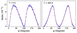
Next, we use the fitted parameters ( from Eq. 1) and look at lower than the saturation field: the FM model (drop the term in Eq. 1) works much worse than the AFM model in Fig. 7(a). This suggests that it is not free magnetic moments (or ferromagnetic inclusions such as MnAs nanocrystals) that responds to but rather, an antiferromagnetic system. It could be that antiferromagnetically coupled pairs of free magnetic moments are responsible for that but given calculated AMR in Tab. 3 it appears likely that we observe bulk response of an antiferromagnet even if it is probably only a fraction of its volume (while its substantial part may be strongly pinned by, for example, structural defects). Another indication that different parts of the system respond differently to is the non-vanishing saturation field at K (see the middle panel of Fig. 4). At this temperature, inferred by SW modelling at saturation nearly vanishes, yet this should be understood as an effect of averaging two or more actual sources of magnetic anisotropy rather than its complete suppression.
V Conclusion
Transport properties experimentally investigated in this work are the magnetoresistance and temperature-dependent resistivity. As for the latter, we find a reasonable agreement between the large structural anisotropy (at low temperatures, the out-of-plane resistivity is almost seven times larger than the in-plane resistivity) and model calculations which show similar, even if typically somewhat smaller, anisotropy regardless of the impurity type. This anisotropy is therefore likely to arise due to layered structure of tetragonal CuMnAs. We encounter frequent violations of Matthiessen rule: for varied concentrations of static impurities, for different types of chemical disorder (at ) and also for phonons and magnons. Anisotropic magnetoresistance (AMR) measured is modest in magnitude and phenomenological modelling indicates the presence of in-plane uniaxial anisotropy which is not oriented along any special crystallographic direction. It is at present impossible to conclude what part of our system responds to the applied magnetic field but it is unlikely that the single-domain picture applies.
Acknowledgements
Discussions with T. Jungwirth and J. Zubáč are acknowledged as well as the support from National Grid Infrastructure MetaCentrum CESNET (No. LM2015042), the Ministry of Education, Youth and Sports from the Large Infrastructures for Research, Experimental Development and Innovations project ’IT4Innovations National Supercomputing Center – LM2015070’, NanoEnviCz (No. LM2015073), Materials Growth and Measurement Laboratory MGML.EU (No. LM2018096, see: http://mgml.eu) all provided under the program ’Projects of Large Research, Development, and Innovations Infrastructures’. I.T., J.K. and D.W. acknowledge financial support by contract Nr. 18-07172S from GAČR, work of JŽ was supported by contract No. 19-18623Y of GAČR and also by the Institute of Physics of the Czech Academy of Sciences and the Max Planck Society through the Max Planck Partner Group programme. P.H. and E.D.N acknowledge funding by ERDF under the project CZ.02.1.01/0.0/0.0/15_003/0000485 and also, EU FET Open RIA Grant No. 766566 and Ministry of Education of the Czech Republic Grant No. LM2018110 and LNSM-LNSpin are acknowledged.
Appendix A Magnetic anisotropies and SW model
Apart from magnetocrystalline anisotropy energy (MAE), lower than cubic symmetry systems are affected by dipolar interactions as far as their easy axes are concerned.Correa:2018_a Using DFT+U calculations,Wadley:2015_a MAE was estimated at 0.130 meV/f.u. favouring the in-plane directions and the dipole-dipole interactions, evaluated using Eq. (A1) of Ref. Correa:2018_a, , further increase the energy penalty for magnetic moments along -axis by 0.04 meV/f.u.
For , lying in-plane, the first term in Eq. (2) can be rewritten using angles , as and the magnetic anisotropy using
| (5) |
where is the easy axis direction. This allows to immediately identify and in Eq. 4 in the case of ferromagnets ( is a reference field). For antiferromagnets, the derivation of Eq. 4 with is more involved. First, the two angles related to are reduced to just one (the one related to canting, i.e. effectively can be expressed analytically and then re-inserted into Eq. 1). Direction of the Néel vector, parametrised by angle , remains as a variable with respect to which the energy should be minimised. Eq. 4 with follows and whereas .
Good fits in Fig. 6 are only possible if we allow for nonzero and, with respect to the [100] crystallographic direction, we find that is inclined by at low temperatures. Biaxial anisotropy can be modelled by replacing with in Eq. (5) but fits give a significantly larger (about a factor of five) than for uniaxial anisotropy. The difference in quality of the fits (uniaxial and biaxial, both with as a free parameter) is also clearly visible.
Appendix B Detailed transport calculations
Tab. 1 of the main text summarizes the most important results for zero-temperature resistivity. However, various approaches (within CPA based on TB-LMTO) to calculate resistivity can be chosen: Tab. 5 gives an overview of both scalar and fully relativistic approaches and the effect of Hubbard and vs. basis is also presented. (We note that data in Tab. 2 are calculated using the basis.) The discrepancies among the values in the table should be considered as an uncertainty of our approach; we note, that a larger basis in the TB-LMTO does not necessary lead to more precise calculations. Resistivities in both Tab. 1 and 5 are shown for 5% of the respective impurity and formation energies are taken from Ref. Maca2019, . In general, the lowest resistivities are obtained for the scalar relativistic approach and the values are also larger for the basis; however, there is no strict trend and various impurities behave differently.
We proceed with a remark on additivity of scattering rates in the context of zero-temperature resistivity. Not only that the Matthiessen rule does not hold for different sources of scattering; even with a single type of impurity, doubling its concentration does not necessarily lead to doubling the resistivity. A clear example of this is shown in Fig. 8. The most striking case is that of non-monotonic with maxima at 7% and 11% of VacMn and VacCu, respectively. In the context of binary alloys, these concentrations are relatively low but similar values have been reported for nonmagnetic Pd-CoKudrnovsky:2015_a and magnetic Ni-Fe and Ni-Co.Turek:2012_a We note, that since these random alloys are cubic, the anisotropy is of minor influence there.
Non-monotonic dependence of on impurity concentration occurs also for the more complex model mentioned in Fig. 2. As a consequence, increasing the concentration ofnote3 Cu does not improve the agreement with experimental data, see Fig. 9. Temperature-dependence of resistance, nevertheless, agrees reasonably well as far as phonons are concerned and this applies to a larger group of impurities. Linear function was fitted to and in the range from 0 K to 180 K and the linear coefficientsnote2 are shown in Tab. 4 Negative values of these coefficients are usually not observed in experiments; nevertheless, measured resistance may decrease with growing chemical disorder and this is also seen in our model results of Fig. 8. Obtained linear coefficients for (shown in Tab. 4) are much more sensitive to the kind of the impurity than in the case of , i.e., the standard deviation of the average value (of the calculated data) is more than 110 % for while similar analysis for gives standard deviation below 30 %. Together with formation energies and residual resistivities (Tab. 1 and 5), the trends may be used to determine the most probable defects.
| Defect | [ cm K-1] | [ cm K-1] |
|---|---|---|
| AsMn | 0.32 0.03 | -0.76 0.06 |
| AsCu | 0.40 0.02 | -0.43 0.14 |
| MnAs | 0.37 0.03 | -0.20 0.03 |
| CuAs | 0.35 0.05 | 0.29 0.11 |
| CuMn | 0.45 0.05 | 0.43 0.10 |
| VacAs | 0.34 0.02 | 0.52 0.17 |
| MnCu | 0.44 0.05 | 0.68 0.01 |
| Cu | 0.47 0.04 | 1.29 0.07 |
| VacCu | 0.48 0.09 | 1.30 0.19 |
| VacMn | 0.46 0.07 | 1.33 0.07 |
| Cu | 0.54 0.05 | 1.51 0.09 |
| Cu | 0.62 0.09 | 1.59 0.18 |
| No impurity | 0.70 0.23 | 1.62 0.41 |
| Experiment | 0.23 0.01 | 1.30 0.02 |
| Formation | Scalar rel., spd | Fully rel., spd | Fully rel., spdf | ||||||||
|---|---|---|---|---|---|---|---|---|---|---|---|
| energy Maca2019 | |||||||||||
| Defect | [eV] | ||||||||||
| Vac | -0.16 | 36 | 155 | 32 | 154 | 19 | 134 | 31 | 184 | 20 | 181 |
| Vac | -0.14 | 12 | 44 | 12 | 54 | 9 | 57 | 16 | 79 | 11 | 92 |
| Mn | -0.03 | 111 | 171 | 115 | 203 | 132 | 683 | 112 | 263 | 150 | 915 |
| Cu | 0.34 | 24 | 122 | 22 | 130 | 8 | 40 | 23 | 131 | 8 | 57 |
| Cu | 1.15 | 107 | 273 | 109 | 377 | 144 | 989 | 121 | 481 | 163 | 1299 |
| As | 1.73 | 94 | 219 | 98 | 257 | 112 | 530 | 114 | 359 | 123 | 694 |
| As | 1.79 | 113 | 262 | 124 | 240 | 133 | 455 | 141 | 476 | 161 | 617 |
| Mn | 1.92 | 122 | 151 | 130 | 270 | 155 | 854 | 147 | 423 | 186 | 1784 |
| Vac | 2.18 | 174 | 203 | 182 | 246 | 219 | 1054 | 210 | 306 | 284 | 1556 |
| CuMn | - | 124 | 267 | 123 | 304 | 127 | 629 | 120 | 393 | 142 | 882 |
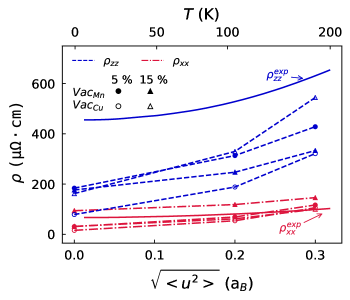
To give another example of phononic effects, we show temperature-dependent resistivity for vacCu and vacMn in Fig. 10. Note that the linear coefficients of in Tab. 4 are in a very good agreement with experimental values for these impurities. Combining Fig. 10 with Fig. 5 leads to different resistivities than what is shown in Fig. 9 thus demonstrating the failure of the Matthiessen rule once again.
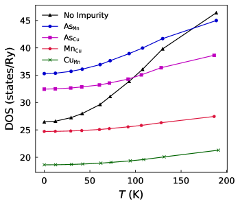
We conclude this appendix by several comments on the correlation of resistivity to the density of states (DOS) at the Fermi level . The saturation of and the decrease of (with increasing temperature) caused by magnons was attributed in Ref. DW2019-JMMM, to a high increase of DOS at the Fermi level. Here we observe decreasing due to phonons for some impurities but having reasonable metallic-like increase. It is shown in Tab. 4 (negative slopes) and in Fig. 5 and we also tried to address it on the level of the DOS. (The energy dependent DOS were calculated, but they are not shown here for brevity; they are presented in Refs. DW2019-JMMM, ; Maca2019, ). For clean stoichiometric CuMnAs, the DOS is strongly increasing above , i.e., there are about twenty states per Ry at , while four times more for eV. Under the presence of phonons, this region of high DOS is smeared (more precisely: large self-energy leads to a large broadening of the spectral function) and for the stoichiometric CuMnAs, situation at is appreciably modified for K (see the black line with crosses in Fig. 11). The drop of in Fig. 5 begins around 200 K which can be expected given the fact that the increase of DOS with temperature is initially compensated by an increase of self-energy. We note that no similar decrease with temperature is observed for ; this could be caused by the layered structure of CuMnAs, but directionally resolved study of the states, e.g., in the terms of the Bloch spectral function similarly to previously investigated NiMnSbDW2019-PRB , is beyond the scope of this paper. Although we attribute the phonon-induced decrease of resistivity to the DOS specific for CuMnAs, it could occur also for other metals having similar DOS.
References
- (1) V. Baltz, A. Manchon, T. Moriyama, T. Ono, and Y. Tserkovnyak, Rev. Mod. Phys. 90, 015005 (2018); T. Jungwirth et al., Nat. Phys. 14, 200 (2018).
- (2) Z. Kašpar et al., arxiv 1909.09071
- (3) P. Wadley et al., Nat. Nanotechn. 13, 362 (2018).
- (4) M. Veis et al., Phys. Rev. B 97, 125109 (2018).
- (5) J. Železný et al., Phys. Rev. Lett. 113, 157201 (2014).
- (6) P. Wadley et al., Science 351, 587 (2016).
- (7) K. Olejník et al., Nat. Comm. (2017). doi: 10.1038/ncomms15434
- (8) P. Wadley et al., Nat. Comm. (2013). doi: 10.1038/ncomms3322
- (9) J. Mundelein and H.U. Schuster, Sect. B J. Chem. Sci 47, 925 (1992).
- (10) F. Krizek et al., Phys. Rev. Mat. 4, 014409 (2020).
- (11) K. Uhlířová et al., J. All. Compd. 650, 224 (2015).
- (12) E. Emmanouilidou et al., Phys. Rev. B 96, 224405 (2017).
- (13) K. Uhlířová et al., J. Alloys Compd. 771, 680 (2019).
- (14) P.J.W. Moll et al., Nat. Commun. 6, 6663 (2015).
- (15) P.J.W. Moll et al., Science 351, 1061 (2016).
- (16) P.J.W. Moll et al., Nature 535, 266 (2016).
- (17) Cu denotes a ’combined’ impurity where a Cu atom is removed from its original position and put at Mn site, i.e. effectively a combination of CuMn and vacCu single-atomic impurities.
- (18) A.W. Rushforth et al., Phys. Rev. Lett. 99, 147207 (2007).
- (19) To be precise, we measured for different directions of rather than different from for the same . Given the tetragonal symmetry, however, the two cases are directly related.
- (20) I. Turek, V. Drchal, J. Kudrnovský, M. Šob, and P. Weinberger: Electronic Structure of Disordered Alloys, Surfaces and Interfaces, 1st ed. (Kluwer Academic Publishers, 1997)
- (21) S.H. Vosko et al., Can. J. Phys. 58, 1200 (1980).
- (22) D. Wagenknecht et al., arxiv 1912.08025 (2019).
- (23) F. Máca et al., Phys. Rev. B 96, 094406 (2017).
- (24) F. Máca et al., J. Magn. Magn. Mat. 474, 467 (2019).
- (25) I. Turek et al., Phys. Rev. B 86, 014405 (2012).
- (26) I. Turek et al., Phys. Rev. B 65, 125101 (2002).
- (27) K. Carva et al., Phys. Rev. B 73, 144421 (2006).
- (28) I. Turek et al., Phys. Rev. B 89, 064405 (2014).
- (29) H. Ebert et al., Phys. Rev. B 91, 165132 (2015).
- (30) D. Ködderitzsch et al., New J. Phys. 15, 053009 (2013).
- (31) J.K. Glasbrenner, B.S. Pujari and K.D. Belashchenko, Phys. Rev. B 89, 174408 (2014).
- (32) A.A. Starikov et al., Phys. Rev. B 97, 214415 (2018).
- (33) D. Wagenknecht, K. Carva and I. Turek, IEEE Transactions on Magnetics 53, 1700205 (2017).
- (34) D. Wagenknecht, K. Carva and I. Turek, Proceedings SPIE (2017), doi: 10.1117/12.2273315.
- (35) D. Wagenknecht et al., J. Magn. Magn. Mat. 474, 517 (2019).
- (36) J. Kudrnovský et al., Phys. Rev. B 86, 144423 (2012).
- (37) D. Wagenknecht et al., Phys. Rev. B 99, 174433 (2019).
- (38) Anton A. Starikov, Yi Liu, Zhe Yuan, and Paul J. Kelly, Phys. Rev. B 97, 214415
- (39) J.B. Staunton et al., Phys. Rev. Lett. 93, 257204 (2004); J.B. Staunton et al., Phys. Rev. B 74, 144411 (2006).
- (40) E.C.Stoner and E.P. Wohlfarth, Phil. Trans. Roy. Soc. A 240 (1948). doi: 10.1098/rsta.1948.0007
- (41) C.A.Correa and K. Výborný, Phys. Rev. B 97, 235111 (2018).
- (42) P. Wadley et al., Sci. Rep. 5, 17079 (2015).
- (43) J. Kudrnovský et al., Phys. Rev. B 92, 224421 (2015).
- (44) Because of finite-temperature scattering mechanism, it would be more appropriate to use a quadratic functionDrchal:2018_a , but we do not have enough data for all of the impurities to perform this analysis reliably and the linear function is sufficient to present trends implied by phonons.
- (45) V. Drchal et al., Phys. Rev. B 98, 134442 (2018).