On efficient numerical solution of linear algebraic systems arising in goal-oriented error estimates

Abstract

We deal with the numerical solution of linear partial differential equations (PDEs) with focus on the goal-oriented error estimates including algebraic errors arising by an inaccurate solution of the corresponding algebraic systems. The goal-oriented error estimates require the solution of the primal as well as dual algebraic systems. We solve both systems simultaneously using the bi-conjugate gradient method which allows to control the algebraic errors of both systems. We develop a stopping criterion which is cheap to evaluate and guarantees that the estimation of the algebraic error is smaller than the estimation of the discretization error. Using this criterion and an adaptive mesh refinement technique, we obtain an efficient and robust method for the numerical solution of PDEs, which is demonstrated by several numerical experiments.

1 Introduction

Let $\Omega\subset{\mathbb{R}}^{d}$ be a polygonal domain with the boundary ${\Gamma}=\partial\Omega$. We consider an abstract partial differential equation in the form

$${\mathscr{L}}{u}=f,$$ (1)

where ${u}:\Omega\to{\mathbb{R}}$ is the unknown solution, ${\mathscr{L}}$ is a linear differential operator and $f$ is the right-hand side. The problem (1) has to be accompanied by suitable boundary conditions. Further, let $V_{h}$ be a finite-dimensional space of functions, ($\dim V_{h}={N_{h}}<\infty$), where an approximation of ${u}$ is sought. We note that the space $V_{h}$ is not given a priori but it is generated as a sequence of spaces by a suitable mesh adaptive method. By ${u_{h}}\in V_{h}$ we denote the discrete solution which approximates $u$.

In many practical application, we are not interested in the solution of (1) itself but rather in a quantity of interest, which is the value of a certain, a priori known, solution-dependent target functional $J({u})$. For example, the functional $J$ is a mean value of the solution over a subset of the computational domain or its boundary. Therefore, we need not to estimate the error ${\left\|{{u}-{u_{h}}}\right\|}$ in an energy norm (cf. AinsworthOden ; verfurth-book2 ) but the error $J(u)-J({u_{h}})$. We assume that $J$ is a linear functional.

The necessity to estimate the error of the target functional gives rise to the goal-oriented error estimates, cf. the pioneering works summarized in RannacherBook ; BeckerRannacher01 ; GileSuli02 . This approach was further developed for many problems, let us mention OdenPrudhomme_CAMWA01 ; Korotov_JCAM06 ; SolDemko04 dealing with linear elliptic problems, KuzminMoller_JCAM10 dealing with steady linear hyperbolic problems. Moreover, extensions to nonlinear problem were presented, e.g., in Rey2Gosselet_CMAME14 ; Rey2Gosselet_CMAME15 for elasticity problems and, e.g., in LoseilleDervieuxAlauzet_JCP10 ; Richter_IJNMF10 ; HH06:SIPG2 ; GeHaHo09 ; Hartman08 ; BalanWoopenMay16 for computational fluid dynamics, for a survey see FidkowskiDarmofal_AIAA11 .

The goal-oriented error estimates require, except the solution of the original (primal) problem (1), also to solve the dual (or adjoint) problem

$${\mathscr{L}}^{*}{z}=J,$$ (2)

where ${\mathscr{L}}^{*}$ is the dual operator to ${\mathscr{L}}$, $J$ is the target functional and ${z}:\Omega\to{\mathbb{R}}$ is the dual solution. The problem (2) has to be accompanied by suitable boundary conditions as well.

It is necessary to approximate the solution of (2) by ${z_{h}^{+}}\in V_{h}^{+}$ where $V_{h}^{+}$ is a richer space than $V_{h}$. One possibility is to discretize (2) directly on $V_{h}^{+}$ (e.g., Korotov_JCAM06 ) but then we have to solve two different algebraic problems. Another way is to discretize (2) on $V_{h}$ and define ${z_{h}^{+}}:={\mathscr{R}}({z_{h}})$, where ${z_{h}}\in V_{h}$ is a numerical approximation of (2) and ${\mathscr{R}}:V_{h}\to V_{h}^{+}$ is a suitable higher order reconstruction (e.g., Richter_IJNMF10 ; CarpioPrietoBermejo_SISC13 ).

The advantage of the latter approach is that the discretizations of the primal and dual problems (1) and (2) using the same space $V_{h}$ are equivalent to two mutually transposed linear algebraic systems which can be beneficial in practical solutions. Namely, we obtain

$$\mathbb{A}\mbox{\boldmath$x$\unboldmath}=\mbox{\boldmath$b$\unboldmath}\qquad\mbox{and}\qquad\mathbb{A}^{{\mkern-1.5mu\mathsf{T}}}\mbox{\boldmath$y$\unboldmath}=\mbox{\boldmath$c$\unboldmath},$$ (3)

where $\mathbb{A}\in{\mathbb{R}}^{{N_{h}}\times{N_{h}}}$ is the matrix arising from the discretization of ${\mathscr{L}}$ from (1), $\mathbb{A}^{{\mkern-1.5mu\mathsf{T}}}$ is the transpose matrix of $\mathbb{A}$, $\mbox{\boldmath$b$\unboldmath}\in{\mathbb{R}}^{{N_{h}}}$ and $\mbox{\boldmath$c$\unboldmath}\in{\mathbb{R}}^{{N_{h}}}$ represent the discretization of the right-hand sides of (1) and (2), respectively, and $\mbox{\boldmath$x$\unboldmath}\in{\mathbb{R}}^{{N_{h}}}$ and $\mbox{\boldmath$y$\unboldmath}\in{\mathbb{R}}^{{N_{h}}}$ are the vectors corresponding to the discrete solutions ${u_{h}}\in V_{h}$ and ${z_{h}}\in V_{h}$ of (1) and (2), respectively.

In many situations, it is advantageous to solve systems (3) iteratively since (i) approximate solutions satisfying the prescribed tolerance are sufficient as an output of the computation; (ii) very good initial approximations of $x$ and $y$ are typically available from previous level of mesh adaptation. Let ${u_{h}^{k}}\in V_{h}$ and ${z_{h}^{k}}\in V_{h}$ denote functions corresponding to the $k$-th iterations $\mbox{\boldmath$x$\unboldmath}_{k}$ and $\mbox{\boldmath$y$\unboldmath}_{k}$, respectively. Then the computed approximations ${u_{h}^{k}}$ and ${z_{h}^{k}}$ are influenced also by the algebraic error arising from the inexact solution of systems (3). Let us note that even if a direct solver for (3) is used then these systems are not solved exactly (only on the level of machine accuracy) and the computed approximations suffers from algebraic errors too, see ArioliLiiesenMiedlerStrakos13 .

Having only approximate solution of (3), the Galerkin orthogonality of the error is violated and many standard a posteriori error estimation techniques can not be used. Therefore, the algebraic error has to be taken into account in a posteriori error analysis. Additionally, the algebraic error estimation is important for the setting of a suitable stopping criterion for iterative solvers and therefore for the optimization of the computational costs. The algebraic error estimates in the framework of energy norms were treated, e.g., in Arioli_NM04 ; Picasso_CNME09 ; VohralikStrakos10 for conforming finite element method in combination with the conjugate gradient method. In the framework of goal-oriented error estimates, a possible violation of Galerkin orthogonality was taken into account, e.g., in KuzminKorotov_MCS10 .

The influence of the algebraic error in goal-oriented error estimates was considered in Meidner2009Goal for iterative algebraic solvers (including multigrid methods). The computational error was expressed and estimated as a sum of the discretization and algebraic errors. The primal and dual algebraic problems (3) were solved alternatively and after some number of iterations (or one multigrid cycle), the algebraic and discretization components of the errors were estimated. Then the iterative process was stopped when the algebraic error estimate was sufficiently smaller than the discretization error estimate. We also mention the recent paper MallikVohralikYousef_JCAM20 using a completely deferent approach for elliptic problems. This technique is based on $H(\mathrm{div})$-conforming flux reconstructions and $H^{1}$-conforming potential reconstructions and yields to a guaranteed upper error bound.

In DolRoskovec_AM17 , we employed an approach similar to Meidner2009Goal and studied the convergence of the error estimator with respect to algebraic iterations of the primal and dual problems. We observed a delay in the convergence for insufficiently accurate resolution of the primal or the dual problem. We arrived to the conclusion that it is difficult to control the efficiency of the computational process when the primal and dual problems (3) are solved alternatively.

Therefore, in this paper, we develop a technique to solve the primal and dual problems (3) simultaneously using the bi-conjugate gradient (BiCG) method. At each BiCG iteration, the approximations of ${u_{h}}$ and ${z_{h}}$ are available and the estimate of the algebraic error can be computed and the accuracy and efficiency can be controlled. Motivated by StTi2011 , we proposed a stopping criterion for the BiCG solver which is very cheap for evaluation and in contrary to Meidner2009Goal ; DolRoskovec_AM17 , it does not require the evaluation of the discretization error estimator. The use of the BiCG solver for the primal and dual problems (3) with the proposed criterion in a combination the mesh adaptation leads to an efficient numerical method for the solution of (1).

Since the presented approach can be applied to (1) with a general linear operator ${\mathscr{L}}$ discretized by any numerical scheme based on a variational formulation, we express the problem considered and its numerical approximation only in the abstract form. However, in order to demonstrate the applicability of this technique, we present the numerical solution of purely elliptic and convection-diffusion problems by the $hp$-adaptive discontinuous Galerkin method (DGM) on possibly anisotropic meshes.

The content of the rest of the paper is the following. In Section 2, we shortly summarize the goal-oriented error estimate technique including two variants of the expression of the algebraic errors. In Section 3, we introduce the algebraic representation of the discrete problems and discuss several ways for the evaluation of the quantity of interest and their corresponding error estimates. These possibilities are numerically tested in Section 4, where we solve the Laplace problem on fixed meshes. Moreover, in Section 5, we describe the mesh adaptation process and proposed new stopping criteria for the BiCG solver. Their computational performance is demonstrated in Section 6 for the Laplace and convection-dominated problems. We conclude with several remarks and discuss a possible extension of this technique for nonlinear problems in Section 7.

2 Framework for the goal-oriented error estimates

We briefly recall a general framework for the goal-oriented error estimates. More details can be found, e.g., in BeckerRannacher01 ; GileSuli02 .

2.1 Primal problem

Let the weak formulation of the primal problem (1) be given by

$$a({u},{\varphi})=\ell({\varphi})\qquad\forall{\varphi}\in V,$$ (4)

where ${u}\in V$ is a weak solution, $a(\cdot,\cdot):V\times V\to{\mathbb{R}}$ is a bilinear form, $\ell(\cdot):V\to{\mathbb{R}}$ is a linear form and $V$ is a Hilbert space. We assume that (4) is well-posed, i.e., it admits a unique weak solution.

For the numerical approximation of (4), let $V_{h},\ h>0$ be a finite element space of functions defined on $\Omega$, typically piecewise polynomial functions related to the partition of $\Omega$ onto a set of finite elements ${{\mathscr{T}}_{h}}$. Moreover, let $W_{h}$ be a functional space such that $V\subset W_{h}$ and $V_{h}\subset W_{h}$. For conforming finite element methods ($V_{h}\subset V$), we simply put $W_{h}:=V$. However, for nonconforming methods (the case $V_{h}\not\subset V$), the choice of $W_{h}$ is more delicate. E.g., for discontinuous Galerkin method, we employ the so-called broken Sobolev space and put

$$W_{h}:=H^{s}({{\mathscr{T}}_{h}})=\{v\in L^{2}(\Omega);\,{\left.\kern-1.2ptv\vphantom{\big{|}}\right|_{K}}\in H^{s}(K)\,\forall K\in{{\mathscr{T}}_{h}}\},$$ (5)

where ${{\mathscr{T}}_{h}}$ is a mesh partition of $\Omega$ and $s>0$ is a suitable Sobolev index, e.g., for the second-order operator ${\mathscr{L}}$, we have $s=2$.

Let

$${a_{h}}:W_{h}\times W_{h}\to{\mathbb{R}}\qquad\mbox{and}\qquad\ell_{h}:W_{h}\to{\mathbb{R}}$$ (6)

be a bilinear and a linear forms corresponding to the discretization of the left-hand and right-hand sides of (4), respectively, by a particular numerical method.

We say that ${u_{h}}\in V_{h}$ is the discrete solution of the primal problem (4) if

$${a_{h}}({u_{h}},{\varphi}_{h})=\ell_{h}({\varphi}_{h})\qquad\forall{\varphi}_{h}\in V_{h}.$$ (7)

We assume that the numerical scheme (7) is consistent, i.e.,

$${a_{h}}({u},{\varphi})=\ell_{h}({\varphi})\qquad\forall{\varphi}\in W_{h}$$ (8)

where ${u}\in V$ is the weak solution of (4). This implies the Galerkin orthogonality of the error of the primal problem

$${a_{h}}({u_{h}}-u,{\varphi}_{h})=0\qquad\forall{\varphi}_{h}\in V_{h}.$$ (9)

Finally, we define the residual of the primal problem by

$$r_{h}({u_{h}})({\varphi}):=\ell_{h}({\varphi})-{a_{h}}({u_{h}},{\varphi})={a_{h}}({u}-{u_{h}},{\varphi}),\quad{\varphi}\in W_{h},$$ (10)

where the last equality follows from the consistency (8).

2.2 Quantity of interest and the dual problem

As mentioned in the introduction, we are interested in a sufficiently accurate approximation of the quantity of interest $J(u)\in{\mathbb{R}}$, where

$$J:W_{h}\to{\mathbb{R}}$$ (11)

is a linear functional. Typically, it is defined as a weighted mean value of $u$ over the computational domain $\Omega$ or its boundary ${\Gamma}$.

In order to estimate the error $J({u})-J({u_{h}})$, we consider the adjoint (or dual) problem (2) and its discretization. We say that ${z_{h}}$ is the discrete solution of the dual problem (2) if

$${a_{h}}(\psi_{h},{z_{h}})=J(\psi_{h})\qquad\forall\psi_{h}\in V_{h},$$ (12)

where ${a_{h}}$ and $J$ are given by (6) and (11), respectively. Moreover, we assume that the numerical scheme (12) is adjoint consistent, i.e.,

$${a_{h}}(\psi,{z})=J(\psi)\qquad\forall\psi\in W_{h},$$ (13)

where ${z}$ is the weak solution of the dual problem (2). This implies the Galerkin orthogonality of the error of the dual problem

$${a_{h}}(\psi_{h},{z_{h}}-{z})=0\qquad\forall\psi_{h}\in V_{h}.$$ (14)

Finally, we define the residual of the dual problem by

$$r_{h}^{*}({z_{h}})(\psi):=J(\psi)-{a_{h}}(\psi,{z_{h}})={a_{h}}(\psi,{z}-{z_{h}}),\quad\psi\in W_{h},$$ (15)

where the last equality follows from the adjoint consistency (13).

The problems (7) and (12) represent two linear algebraic systems whose efficient solution by an iterative solver is developed in Section 3. Due to iterative and rounding errors, the “exact” discrete solutions ${u_{h}}$ and ${z_{h}}$ are not available, we have only their approximation ${u_{h}^{k}}\in V_{h}$ and ${z_{h}^{k}}\in V_{h}$, $k=1,2,\dots$. However, they do not fulfil the Galerkin orthogonalities (9) and (14).

2.3 Abstract goal-oriented error estimates

Obviously, for adjoint consistent discretization we have (due to (8) and (13)) the equivalence between the quantity of interest $J({u})$ and the right-hand side of (4) evaluated for the dual solution ${z},$ i.e.

$$\ell_{h}({z})={a_{h}}({u},{z})=J({u}).$$ (16)

Similarly, from (7) and (12), we obtain the discrete variant of (16) as

$$\ell_{h}({z_{h}})={a_{h}}({u_{h}},{z_{h}})=J({u_{h}}),$$ (17)

where ${u_{h}}$ and ${z_{h}}$ are the discrete solutions of the primal and dual problems, respectively. Consequently, we have an error equivalence

$$J({u}-{u_{h}})=J({u})-J({u_{h}})=\ell_{h}({z})-\ell_{h}({z_{h}})=\ell_{h}({z}-{z_{h}}).$$ (18)

Therefore, the difference $\ell_{h}({z}-{z_{h}})$ can be used as an error estimate of the quantity of interest as well.

First, we present the primal and dual error identities for the error of the quantity of interest for the algebraically exact discrete solution ${u_{h}}$ and ${z_{h}}$ of (7) and (12), respectively. Using the adjoint consistency (13), the Galerkin orthogonality (9) and relation (10), we get the primal error identity

$$J({u}-{u_{h}}) ={a_{h}}({u}-{u_{h}},{z})={a_{h}}({u}-{u_{h}},{z}-v_{h})$$ (19)

$$=r_{h}({u_{h}})({z}-v_{h})\quad\forall v_{h}\in V_{h},$$

where $r_{h}({z_{h}})(\cdot)$ denotes the residual of the primal problem given by (10).

Similarly, exploiting in addition the Galerkin orthogonality (14) and relation (15), we get the dual error identity

$$J({u}-{u_{h}}) ={a_{h}}({u}-{u_{h}},{z}-{z_{h}})={a_{h}}({u}-w_{h},{z}-{z_{h}})$$ (20)

$$=r_{h}^{*}({z_{h}})({u}-w_{h})\quad\forall w_{h}\in V_{h},$$

where $r_{h}^{*}({z_{h}})(\cdot)$ denotes the residual of the dual problem given by (15).

2.4 Abstract goal-oriented error estimates including algebraic errors

As mentioned above, the discrete solutions ${u_{h}}$ and ${z_{h}}$ fulfilling (7) and (12), respectively, are non-available but we have only ${u_{h}^{k}}\in V_{h}$ and ${z_{h}^{k}}\in V_{h}$, $k=1,2,\dots$ denoting their approximations given by an algebraic iterative solver. Hence, the error representations (19) and (20) are useless and we have to estimate the error $J({u}-{u_{h}^{k}})$.

In the same way as in Meidner2009Goal ; DolRoskovec_AM17 , we employ the adjoint consistency (13), identity ${z}={z}-v_{h}+v_{h},\ v_{h}\in V_{h}$ and relation (10), we get the primal error identity including algebraic errors

$$J({u}-{u_{h}^{k}}) ={a_{h}}({u}-{u_{h}^{k}},{z})={a_{h}}({u}-{u_{h}^{k}},{z}-v_{h})+{a_{h}}({u}-{u_{h}^{k}},v_{h})$$ (21)

$$=r_{h}({u_{h}^{k}})({z}-v_{h})+r_{h}({u_{h}^{k}})(v_{h})\quad\forall v_{h}\in V_{h},$$

where $r_{h}({u_{h}^{k}})(\cdot)$ is given by (10). Inserting $v_{h}:={z_{h}^{k}}$ in (21), we obtain

$$J({u}-{u_{h}^{k}})=r_{h}({u_{h}^{k}})({z}-{z_{h}^{k}})+r_{h}({u_{h}^{k}})({z_{h}^{k}})=:{e_{\mathrm{S},k}}+{e_{\mathrm{A},k}},$$ (22)

where the quantity ${e_{\mathrm{S},k}}=r_{h}({u_{h}^{k}})({z}-{z_{h}^{k}})$ represents the discretization error of the primal problem since it coincides with (19) for ${u_{h}^{k}}={u_{h}}$. Further, the quantity ${e_{\mathrm{A},k}}=r_{h}({u_{h}^{k}})({z_{h}^{k}})$ represents the algebraic error of the primal problem since it vanishes for ${u_{h}^{k}}={u_{h}}$. Let us note that (21) and (22) hold without the Galerkin orthogonality (9).

In order to derive the analogue of (20) including algebraic error, we take into account the error equivalence (18). The quantity $\ell_{h}({z}-{z_{h}^{k}})$ exhibits the analogue of the error $J({u}-{u_{h}^{k}})$ since both quantities are equal for ${u_{h}^{k}}={u_{h}}$ and ${z_{h}^{k}}={z_{h}}$. However, if ${u_{h}^{k}}$ and ${z_{h}^{k}}$ are arbitrary iterations then, in general,

$$J({u}-{u_{h}^{k}})\not=\ell_{h}({z}-{z_{h}^{k}}).$$ (23)

Nevertheless, we show in Section 3 (cf. (64)) that if ${u_{h}^{k}}$ and ${z_{h}^{k}}$ are obtained by the bi-conjugate gradient (BiCG) method with vanishing initial approximations (in the exact arithmetic) then

$$J({u}-{u_{h}^{k}})=\ell_{h}({z}-{z_{h}^{k}})\qquad\mbox{ for }k=1,2,\dots.$$ (24)

Now, using the consistency (13), identity ${z}={z}-w_{h}+w_{h},\ w_{h}\in V_{h}$ and relation (10), we get the dual error identity including algebraic errors

$$\ell_{h}({z}-{z_{h}^{k}}) ={a_{h}}({u},{z}-{z_{h}^{k}})={a_{h}}({u}-w_{h},{z}-{z_{h}^{k}})+{a_{h}}(w_{h},{z}-{z_{h}^{k}})$$ (25)

$$=r_{h}^{*}({z_{h}^{k}})({u}-w_{h})+r_{h}^{*}({z_{h}^{k}})(w_{h})\quad\forall w_{h}\in V_{h},$$

where $r_{h}^{*}({z_{h}^{k}})(\cdot)$ is given by (15). Putting $w_{h}:={u_{h}^{k}}$ in (25), we obtain

$$\ell_{h}({z}-{z_{h}^{k}})=r_{h}^{*}({z_{h}^{k}})({u}-{u_{h}^{k}})+r_{h}^{*}({z_{h}^{k}})({u_{h}^{k}})=:{e_{\mathrm{S},k}^{*}}+{e_{\mathrm{A},k}^{*}},$$ (26)

where, similarly as the quantities ${e_{\mathrm{S},k}}$ and ${e_{\mathrm{A},k}}$ in (22), the quantities ${e_{\mathrm{S},k}^{*}}$ and ${e_{\mathrm{A},k}^{*}}$ represent the discretization and algebraic error of the dual problem. Let us note that (25) and (26) hold without the Galerkin orthogonality (14).

2.5 Computable goal-oriented error estimates

Whereas the algebraic errors ${e_{\mathrm{A},k}}$ and ${e_{\mathrm{A},k}^{*}}$ from (22) and (26), respectively, are computable quantities, the discretization errors ${e_{\mathrm{S},k}}$ and ${e_{\mathrm{S},k}^{*}}$ require the knowledge of the exact dual and primal and solutions ${z}$ and ${u}$, respectively. In practical computations, they should be approximated by a higher-order reconstruction denoted here by

$${{u}_{h}^{+}}={\mathscr{R}}({u_{h}^{k}}),\qquad{{z}_{h}^{+}}={\mathscr{R}}({z_{h}^{k}}),$$ (27)

where ${u_{h}^{k}}\in V_{h}$ and ${z_{h}^{k}}\in V_{h}$ denote approximations of ${u_{h}}$ and ${z_{h}}$, ${\mathscr{R}}:V_{h}\to V_{h}^{+}$ denotes a reconstruction operator and $V_{h}^{+}$ is a “richer” finite dimensional space, for examples, see the papers cited in Introduction.

Replacing ${u}$ and ${z}$ in (22) and (26) by ${{u}_{h}^{+}}$ and ${{z}_{h}^{+}}$, we obtain the computable approximations $\eta_{\mathrm{S},k}$ and $\eta_{\mathrm{S},k}^{*}$ of the discretization errors ${e_{\mathrm{S},k}}$ and ${e_{\mathrm{S},k}^{*}}$ by

$${e_{\mathrm{S},k}}=r_{h}({u_{h}^{k}})({z}-{z_{h}^{k}})\approx r_{h}({u_{h}^{k}})({{z}_{h}^{+}}-{z_{h}^{k}})=:\eta_{\mathrm{S},k},$$ (28)

$${e_{\mathrm{S},k}^{*}}=r_{h}^{*}({z_{h}^{k}})({u}-{u_{h}^{k}})\approx r_{h}({z_{h}^{k}})({{u}_{h}^{+}}-{u_{h}^{k}})=:\eta_{\mathrm{S},k}^{*},\qquad k=1,2,\dots.$$

The quantities $\eta_{\mathrm{S},k}$ and $\eta_{\mathrm{S},k}^{*}$ are called the estimates of the primal and dual discretization errors, respectively.

The approximations (28) together with (22) and (26) lead to the computable estimate of the total error by

$$J({u}-{u_{h}^{k}}) \approx\eta_{\mathrm{S},k}+\eta_{\mathrm{A},k},\qquad\ell_{h}({z}-{z_{h}^{k}})\approx\eta_{\mathrm{S},k}^{*}+\eta_{\mathrm{A},k}^{*},\quad k=1,2,\dots,$$ (29)

where, in order to have a consistent notation, we put

$$\eta_{\mathrm{A},k}:={e_{\mathrm{A},k}}=r_{h}({u_{h}^{k}})({z_{h}^{k}}),\quad\eta_{\mathrm{A},k}^{*}:={e_{\mathrm{A},k}^{*}}=r_{h}^{*}({z_{h}^{k}})({u_{h}^{k}}).$$ (30)

The terms $\eta_{\mathrm{A},k}$ and $\eta_{\mathrm{A},k}^{*}$ are equal to the algebraic errors of the primal and dual problems (7) and (12), respectively, and they are independent on the used higher-order reconstruction ${\mathscr{R}}$ from (27).

Remark 1

The approximations (29) do not give a guaranteed error estimate since, as usual, we neglected the terms $r_{h}({u_{h}^{k}})({z}-{{z}_{h}^{+}})$ and $r_{h}({z_{h}^{k}})({u}-{{u}_{h}^{+}})$. Hence, the guaranteed error estimate requires an estimation of these terms. We refer to NochettoVeeserVerani_IMAJNA09 ; Ainsworth2012Guaranteed where this problem was treated for symmetric elliptic problems discretized by the conforming finite element method. This is also a subject of our further research.

2.6 An alternative representation of the algebraic error

In (22), we expressed the discretization and algebraic parts of the computational error using the approach from Meidner2009Goal , namely

$$J({u}-{u_{h}^{k}})=r_{h}({u_{h}^{k}})({z}-{z_{h}^{k}})+r_{h}({u_{h}^{k}})({z_{h}^{k}})={e_{\mathrm{S},k}}+{e_{\mathrm{A},k}}.$$ (31)

On the other hand, it is possible to decompose the total error $J({u}-{u_{h}^{k}})$ in the alternative way as

$$J({u}-{u_{h}^{k}})=J({u}-{u_{h}})+J({u_{h}}-{u_{h}^{k}})=:\zeta_{\mathrm{S},k}+\zeta_{\mathrm{A},k}.$$ (32)

The first term in (32) is the discretization error given by (19) and it satisfies

$$\zeta_{\mathrm{S},k}=J({u}-{u_{h}})=r_{h}({u_{h}})({z}-v_{h}),\quad v_{h}\in V_{h}$$ (33)

and it is independent of $k$. Obviously, although ${e_{\mathrm{S},k}}$ in (31) and $\zeta_{\mathrm{S},k}$ in (33) both represent the discretization error, they differ. Moreover, $\zeta_{\mathrm{S},k}$ cannot be evaluated even if we replace ${z}$ by ${{z}_{h}^{+}}$ since ${u_{h}}$ is unavailable.

The second term $\zeta_{\mathrm{A},k}$ in (32) represents the algebraic error. It cannot be expressed in a residual form but in Section 3, we present a technique which is able to estimate this term in a cheap way.

Hence, we have two representations of the algebraic error, the first one from (31) given by $\eta_{\mathrm{A},k}=r_{h}({u_{h}^{k}})({z_{h}^{k}})$ and the second one from (32) given by $\zeta_{\mathrm{A},k}:=J({u_{h}}-{u_{h}^{k}})$. Both representations are “algebraically consistent” which means that if ${u_{h}^{k}}\to{u_{h}}$ and ${z_{h}^{k}}\to{z_{h}}$ for $k\to\infty$ then

$$\eta_{\mathrm{A},k}\to 0\quad\mbox{ for }k\to\infty\qquad\mbox{ and }\qquad\zeta_{\mathrm{A},k}\to 0\quad\mbox{ for }k\to\infty.$$ (34)

However, the speed of convergence for $\eta_{\mathrm{A},k}$ and $\zeta_{\mathrm{A},k}$ can differ substantially, see numerical experiments in Section 6.

Moreover, for ${u_{h}^{k}}\to{u_{h}}$ and ${z_{h}^{k}}\to{z_{h}}$, both discretization errors ${e_{\mathrm{S},k}}$ and $\zeta_{\mathrm{S},k}$ are closer and closer since (cf. (31) and (32))

$$|{e_{\mathrm{S},k}}-\zeta_{\mathrm{S},k}|=|\zeta_{\mathrm{A},k}-{e_{\mathrm{A},k}}|\leq|\zeta_{\mathrm{A},k}|+|{e_{\mathrm{A},k}}|\to 0.$$ (35)

Finally, we present the dual analogue of (32)–(33) in the form

$$\ell_{h}({z}-{z_{h}^{k}}) =\ell_{h}({z}-{z_{h}})+\ell_{h}({z_{h}}-{z_{h}^{k}})=:\zeta_{\mathrm{S},k}^{*}+\zeta_{\mathrm{A},k}^{*},$$ (36)

where the term $\zeta_{\mathrm{A},k}^{*}$ can be estimated in the same manner as $\zeta_{\mathrm{A},k}$ in (32), cf. Section 3.

3 Solution of primal and dual discretized problems

In this section, we introduce the algebraic representation of the goal-oriented error estimates from the previous section, present the BiCG method allowing a simultaneous solution of the primal and dual problems and discuss several possibilities algebraic errors estimates and stopping criteria for the iterative solver.

3.1 Algebraic representation

Let $\{{\varphi}_{i}:\Omega\to{\mathbb{R}},\ i=1,\dots,{N_{h}}\}$ be a basis of the finite-dimensional space $V_{h}$. We define the matrix $\mathbb{A}\in{\mathbb{R}}^{{N_{h}}\times{N_{h}}}$ by

$$\mathbb{A}=\{\mathbb{A}_{i,j}\}_{i,j=1}^{{N_{h}}},\quad\mathbb{A}_{i,j}:={a_{h}}({\varphi}_{i},{\varphi}_{j}),\ i,j=1,\dots,{N_{h}},$$ (37)

where ${a_{h}}$ is the bilinear form defined by (6). Then the primal and dual discrete problems (7) and (12) are equivalent to the solution of two linear algebraic systems

$$\mathbb{A}\mbox{\boldmath$x$\unboldmath}=\mbox{\boldmath$b$\unboldmath}\qquad\mbox{and}\qquad\mathbb{A}^{{\mkern-1.5mu\mathsf{T}}}\mbox{\boldmath$y$\unboldmath}=\mbox{\boldmath$c$\unboldmath},$$ (38)

respectively, where $\mbox{\boldmath$x$\unboldmath}\in{\mathbb{R}}^{N_{h}}$ and $\mbox{\boldmath$y$\unboldmath}\in{\mathbb{R}}^{N_{h}}$ are the algebraic representation of the primal and dual solutions given by

$$\mbox{\boldmath$x$\unboldmath}=(x_{1},\dots,x_{{N_{h}}})^{{\mkern-1.5mu\mathsf{T}}}\ \leftrightarrow{u_{h}}=\sum\nolimits_{i=1}^{N_{h}}x_{i}{\varphi}_{i},$$ (39)

and $$\mbox{\boldmath$y$\unboldmath}=(y_{1},\dots,y_{{N_{h}}})^{{\mkern-1.5mu\mathsf{T}}}\ \leftrightarrow{z_{h}}=\sum\nolimits_{i=1}^{N_{h}}y_{i}{\varphi}_{i},$$

respectively, and $\mbox{\boldmath$b$\unboldmath}\in{\mathbb{R}}^{N_{h}}$ and $\mbox{\boldmath$c$\unboldmath}\in{\mathbb{R}}^{N_{h}}$ are the algebraic representation of the right-hand sides of the primal and dual problems given by

$$\mbox{\boldmath$b$\unboldmath}=(b_{1},\dots,b_{{N_{h}}})^{{\mkern-1.5mu\mathsf{T}}}\ \leftrightarrow b_{i}=\ell_{h}({\varphi}_{i}),\ i=1,\dots,{N_{h}},$$ (40)

and $$\mbox{\boldmath$c$\unboldmath}=(c_{1},\dots,c_{{N_{h}}})^{{\mkern-1.5mu\mathsf{T}}}\ \leftrightarrow c_{i}=J({\varphi}_{i}),\quad i=1,\dots,{N_{h}},$$

respectively. Using (37)–(40), we obtain the equivalencies

$$J({u_{h}}) =\sum_{i=1}^{N_{h}}x_{i}J({\varphi}_{i})=\mbox{\boldmath$c$\unboldmath}^{{\mkern-1.5mu\mathsf{T}}}\mbox{\boldmath$x$\unboldmath}=\mbox{\boldmath$c$\unboldmath}^{{\mkern-1.5mu\mathsf{T}}}\mathbb{A}^{-1}\mbox{\boldmath$b$\unboldmath}=\mbox{\boldmath$y$\unboldmath}^{{\mkern-1.5mu\mathsf{T}}}\mbox{\boldmath$b$\unboldmath}=\sum_{i=1}^{{N_{h}}}y_{i}\ell_{h}({\varphi}_{i})=\ell_{h}({z_{h}}),$$ (41)

which exhibits the algebraic analogue of (17).

Similarly, as in (39) let $\mbox{\boldmath$x$\unboldmath}_{k}$ and $\mbox{\boldmath$y$\unboldmath}_{k}$ be the algebraic analogues of the approximations ${u_{h}^{k}}$ and ${z_{h}^{k}}$, respectively. The corresponding residuals of (38) are given by

$$\mbox{\boldmath$r$\unboldmath}_{k}:=\mbox{\boldmath$b$\unboldmath}-\mathbb{A}\mbox{\boldmath$x$\unboldmath}_{k}=\mathbb{A}(\mbox{\boldmath$x$\unboldmath}-\mbox{\boldmath$x$\unboldmath}_{k})\quad\mbox{ and }\quad\mbox{\boldmath$s$\unboldmath}_{k}:=\mbox{\boldmath$c$\unboldmath}-\mathbb{A}^{{\mkern-1.5mu\mathsf{T}}}\mbox{\boldmath$y$\unboldmath}_{k}=\mathbb{A}^{{\mkern-1.5mu\mathsf{T}}}(\mbox{\boldmath$y$\unboldmath}-\mbox{\boldmath$y$\unboldmath}_{k}).$$ (42)

By a standard manipulation, we derive the following correspondence between the discretization and its algebraic representation which will be used in next paragraphs. Similarly as in (41), we have

$$J({u_{h}^{k}}) =\mbox{\boldmath$c$\unboldmath}^{{\mkern-1.5mu\mathsf{T}}}\mbox{\boldmath$x$\unboldmath}_{k},\qquad\ell_{h}({z_{h}^{k}})=\mbox{\boldmath$y$\unboldmath}_{k}^{{\mkern-1.5mu\mathsf{T}}}\mbox{\boldmath$b$\unboldmath}.$$ (43)

From (37) and (39), we obtain

$${a_{h}}({u_{h}^{k}},{z_{h}^{k}}) =\mbox{\boldmath$y$\unboldmath}_{k}^{{\mkern-1.5mu\mathsf{T}}}\mathbb{A}\mbox{\boldmath$x$\unboldmath}_{k}.$$ (44)

Additionally, employing (38) and (42), we derive

$${a_{h}}({u_{h}}-{u_{h}^{k}},{z_{h}}-{z_{h}^{k}}) =(\mbox{\boldmath$y$\unboldmath}-\mbox{\boldmath$y$\unboldmath}_{k})^{{\mkern-1.5mu\mathsf{T}}}\mathbb{A}(\mbox{\boldmath$x$\unboldmath}-\mbox{\boldmath$x$\unboldmath}_{k})=\mbox{\boldmath$s$\unboldmath}_{k}^{{\mkern-1.5mu\mathsf{T}}}\mathbb{A}^{-1}\mbox{\boldmath$r$\unboldmath}_{k}.$$ (45)

Finally, using (10), (15), (30) and (42)–(44), we obtain

$$\eta_{\mathrm{A},k} =\ell({z_{h}^{k}})-{a_{h}}({u_{h}^{k}},{z_{h}^{k}})=\mbox{\boldmath$y$\unboldmath}_{k}^{{\mkern-1.5mu\mathsf{T}}}\mbox{\boldmath$b$\unboldmath}-\mbox{\boldmath$y$\unboldmath}_{k}^{{\mkern-1.5mu\mathsf{T}}}\mathbb{A}\mbox{\boldmath$x$\unboldmath}_{k}=\mbox{\boldmath$y$\unboldmath}_{k}^{{\mkern-1.5mu\mathsf{T}}}\mbox{\boldmath$r$\unboldmath}_{k},$$ (46)

$$\eta_{\mathrm{A},k}^{*} =J({u_{h}^{k}})-{a_{h}}({u_{h}^{k}},{z_{h}^{k}})=\mbox{\boldmath$c$\unboldmath}^{{\mkern-1.5mu\mathsf{T}}}\mbox{\boldmath$x$\unboldmath}_{k}-\mbox{\boldmath$y$\unboldmath}_{k}^{{\mkern-1.5mu\mathsf{T}}}\mathbb{A}\mbox{\boldmath$x$\unboldmath}_{k}=\mbox{\boldmath$s$\unboldmath}_{k}^{{\mkern-1.5mu\mathsf{T}}}\mbox{\boldmath$x$\unboldmath}_{k}.$$

3.2 Approximating the quantity of interest using iterates $\mbox{\boldmath$x$\unboldmath}_{k}$ and $\mbox{\boldmath$y$\unboldmath}_{k}$

Let the approximations $\mbox{\boldmath$x$\unboldmath}_{k}$ and $\mbox{\boldmath$y$\unboldmath}_{k}$, and the corresponding residual vectors $\mbox{\boldmath$r$\unboldmath}_{k}$ and $\mbox{\boldmath$s$\unboldmath}_{k}$, computed by some iterative method for solving linear systems (38), be given. We introduce several possibilities, how to approximate the quantity of interest $J({u_{h}})=\mbox{\boldmath$c$\unboldmath}^{{\mkern-1.5mu\mathsf{T}}}\mathbb{A}^{-1}\mbox{\boldmath$b$\unboldmath}=\ell_{h}({z_{h}})$ using these vectors. For each possibility, we express the quantity of interest as a sum of two terms, where the former one is a computable value approximating the quantity of interest and the latter one is an incomputable term which represents the error of the approximation. Note that the identities derived below rely only on the relations

$$\mbox{\boldmath$r$\unboldmath}_{k}=\mbox{\boldmath$b$\unboldmath}-\mathbb{A}\mbox{\boldmath$x$\unboldmath}_{k}\quad\mbox{ and }\quad\mbox{\boldmath$s$\unboldmath}_{k}=\mbox{\boldmath$c$\unboldmath}-\mathbb{A}^{{\mkern-1.5mu\mathsf{T}}}\mbox{\boldmath$y$\unboldmath}_{k}.$$ (47)

• Using (42), a simple manipulation gives

  $$\mbox{\boldmath$c$\unboldmath}^{{\mkern-1.5mu\mathsf{T}}}\mathbb{A}^{-1}\mbox{\boldmath$b$\unboldmath}=\mbox{\boldmath$c$\unboldmath}^{{\mkern-1.5mu\mathsf{T}}}\mbox{\boldmath$x$\unboldmath}=\mbox{\boldmath$c$\unboldmath}^{{\mkern-1.5mu\mathsf{T}}}\mbox{\boldmath$x$\unboldmath}_{k}+\mbox{\boldmath$c$\unboldmath}^{{\mkern-1.5mu\mathsf{T}}}(\mbox{\boldmath$x$\unboldmath}-\mbox{\boldmath$x$\unboldmath}_{k})=\underbrace{\mbox{\boldmath$c$\unboldmath}^{{\mkern-1.5mu\mathsf{T}}}\mbox{\boldmath$x$\unboldmath}_{k}}_{\mathrm{approximation}}+\underbrace{\mbox{\boldmath$c$\unboldmath}^{{\mkern-1.5mu\mathsf{T}}}\mathbb{A}^{-1}\mbox{\boldmath$r$\unboldmath}_{k}}_{\mathrm{error}}.$$ (48)

  The first term on the right-hand side of (48) is computable and then it can be used for the approximation $\mbox{\boldmath$c$\unboldmath}^{{\mkern-1.5mu\mathsf{T}}}\mathbb{A}^{-1}\mbox{\boldmath$b$\unboldmath}\approx\mbox{\boldmath$c$\unboldmath}^{{\mkern-1.5mu\mathsf{T}}}\mbox{\boldmath$x$\unboldmath}_{k}$ and the second term $\mbox{\boldmath$c$\unboldmath}^{{\mkern-1.5mu\mathsf{T}}}\mathbb{A}^{-1}\mbox{\boldmath$r$\unboldmath}_{k}$ represents the corresponding error. Similarly, for the dual form, we have

  $$\mbox{\boldmath$c$\unboldmath}^{{\mkern-1.5mu\mathsf{T}}}\mathbb{A}^{-1}\mbox{\boldmath$b$\unboldmath}=\mbox{\boldmath$y$\unboldmath}^{{\mkern-1.5mu\mathsf{T}}}\mbox{\boldmath$b$\unboldmath}=\mbox{\boldmath$y$\unboldmath}_{k}^{{\mkern-1.5mu\mathsf{T}}}\mbox{\boldmath$b$\unboldmath}+(\mbox{\boldmath$y$\unboldmath}-\mbox{\boldmath$y$\unboldmath}_{k})^{{\mkern-1.5mu\mathsf{T}}}\mbox{\boldmath$b$\unboldmath}=\underbrace{\mbox{\boldmath$y$\unboldmath}_{k}^{{\mkern-1.5mu\mathsf{T}}}\mbox{\boldmath$b$\unboldmath}}_{\mathrm{approximation}}+\underbrace{\mbox{\boldmath$s$\unboldmath}_{k}^{{\mkern-1.5mu\mathsf{T}}}\mathbb{A}^{-1}\mbox{\boldmath$b$\unboldmath}}_{\mathrm{error}},$$ (49)

  thus $\mbox{\boldmath$y$\unboldmath}_{k}^{{\mkern-1.5mu\mathsf{T}}}\mbox{\boldmath$b$\unboldmath}$ is a computable approximation of $\mbox{\boldmath$c$\unboldmath}^{{\mkern-1.5mu\mathsf{T}}}\mathbb{A}^{-1}\mbox{\boldmath$b$\unboldmath}$ and $\mbox{\boldmath$s$\unboldmath}_{k}^{{\mkern-1.5mu\mathsf{T}}}\mathbb{A}^{-1}\mbox{\boldmath$b$\unboldmath}$ the corresponding error.

• We carry out more sophisticated manipulation, take into account (38), (42), (45) and get

  $$\mbox{\boldmath$c$\unboldmath}^{{\mkern-1.5mu\mathsf{T}}}\mathbb{A}^{-1}\mbox{\boldmath$b$\unboldmath} =\mbox{\boldmath$c$\unboldmath}^{{\mkern-1.5mu\mathsf{T}}}\mbox{\boldmath$x$\unboldmath}_{k}+\mbox{\boldmath$c$\unboldmath}^{{\mkern-1.5mu\mathsf{T}}}\mathbb{A}^{-1}\mathbb{A}(\mbox{\boldmath$x$\unboldmath}-\mbox{\boldmath$x$\unboldmath}_{k})=\mbox{\boldmath$c$\unboldmath}^{{\mkern-1.5mu\mathsf{T}}}\mbox{\boldmath$x$\unboldmath}_{k}+\mbox{\boldmath$y$\unboldmath}^{{\mkern-1.5mu\mathsf{T}}}\mathbb{A}(\mbox{\boldmath$x$\unboldmath}-\mbox{\boldmath$x$\unboldmath}_{k})$$ (50)

  $$=\mbox{\boldmath$c$\unboldmath}^{{\mkern-1.5mu\mathsf{T}}}\mbox{\boldmath$x$\unboldmath}_{k}+\mbox{\boldmath$y$\unboldmath}_{k}^{{\mkern-1.5mu\mathsf{T}}}(\mbox{\boldmath$b$\unboldmath}-\mathbb{A}\mbox{\boldmath$x$\unboldmath}_{k})+(\mbox{\boldmath$y$\unboldmath}-\mbox{\boldmath$y$\unboldmath}_{k})^{{\mkern-1.5mu\mathsf{T}}}\mathbb{A}(\mbox{\boldmath$x$\unboldmath}-\mbox{\boldmath$x$\unboldmath}_{k})$$

  $$=\underbrace{\mbox{\boldmath$c$\unboldmath}^{{\mkern-1.5mu\mathsf{T}}}\mbox{\boldmath$x$\unboldmath}_{k}+\mbox{\boldmath$y$\unboldmath}_{k}^{{\mkern-1.5mu\mathsf{T}}}\mbox{\boldmath$r$\unboldmath}_{k}}_{\mathrm{approximation}}+\underbrace{\mbox{\boldmath$s$\unboldmath}_{k}^{{\mkern-1.5mu\mathsf{T}}}\mathbb{A}^{-1}\mbox{\boldmath$r$\unboldmath}_{k}}_{\mathrm{error}}.$$

  Using the algebraic-discretization equivalence relations (41), (43), (45) and (46), the identity (50) can be written in the equivalent form

  $$J({u_{h}})=\underbrace{J({u_{h}^{k}})+\eta_{\mathrm{A},k}}_{\mathrm{approximation}}+\underbrace{{a_{h}}({u_{h}}-{u_{h}^{k}},{z_{h}}-{z_{h}^{k}})}_{\mathrm{error}}.$$ (51)

  Similarly, we can derive the dual relation

  $$\mbox{\boldmath$c$\unboldmath}^{{\mkern-1.5mu\mathsf{T}}}\mathbb{A}^{-1}\mbox{\boldmath$b$\unboldmath}=\underbrace{\mbox{\boldmath$y$\unboldmath}_{k}^{{\mkern-1.5mu\mathsf{T}}}\mbox{\boldmath$b$\unboldmath}+\mbox{\boldmath$s$\unboldmath}_{k}^{{\mkern-1.5mu\mathsf{T}}}\mbox{\boldmath$x$\unboldmath}_{k}}_{\mathrm{approximation}}+\underbrace{\mbox{\boldmath$s$\unboldmath}_{k}^{{\mkern-1.5mu\mathsf{T}}}\mathbb{A}^{-1}\mbox{\boldmath$r$\unboldmath}_{k}}_{\mathrm{error}},$$ (52)

  which is equivalent to

  $$\ell_{h}({z_{h}})=\underbrace{\ell_{h}({z_{h}^{k}})+\eta_{\mathrm{A},k}^{*}}_{\mathrm{approximation}}+\underbrace{{a_{h}}({u_{h}}-{u_{h}^{k}},{z_{h}}-{z_{h}^{k}})}_{\mathrm{error}}.$$ (53)

As mentioned at the beginning of this section, both evaluations (P1) and (P2) can be used for any iterative solver generating approximations $\mbox{\boldmath$x$\unboldmath}_{k}$ and $\mbox{\boldmath$y$\unboldmath}_{k}$, and residuals $\mbox{\boldmath$r$\unboldmath}_{k}$ and $\mbox{\boldmath$s$\unboldmath}_{k}$, $k=1,2,\dots$. If the norms of the residual vectors $\mbox{\boldmath$r$\unboldmath}_{k}$ and $\mbox{\boldmath$s$\unboldmath}_{k}$ tend to be small, one can expect that

$$|\mbox{\boldmath$s$\unboldmath}_{k}^{{\mkern-1.5mu\mathsf{T}}}\mathbb{A}^{-1}\mbox{\boldmath$r$\unboldmath}_{k}|\ll|\mbox{\boldmath$c$\unboldmath}^{{\mkern-1.5mu\mathsf{T}}}\mathbb{A}^{-1}\mbox{\boldmath$r$\unboldmath}_{k}|\qquad\mbox{and}\qquad|\mbox{\boldmath$s$\unboldmath}_{k}^{{\mkern-1.5mu\mathsf{T}}}\mathbb{A}^{-1}\mbox{\boldmath$r$\unboldmath}_{k}|\ll|\mbox{\boldmath$s$\unboldmath}_{k}^{{\mkern-1.5mu\mathsf{T}}}\mathbb{A}^{-1}\mbox{\boldmath$b$\unboldmath}|.$$ (54)

In other words, one can expect that the approximation (P2) is more accurate than (P1) since the corresponding error terms tend to be smaller.

3.3 Approximating the quantity of interest using BiCG iterates

As mentioned in Introduction, our aim is to solve systems (38) by an iterative method, which allows to solve the primal and dual problems simultaneously. Since we intend to solve large and sparse systems, we need to pick a method with low memory requirements. Then, a natural choice is to use the preconditioned bi-conjugate gradient (BiCG) method (Algorithm 1) introduced in Fl1976 ; see also B:BaBeCh1994 ; StTi2011 . Let $\mathbb{P}$ be a suitable preconditioner (its choice depends on the particular discretization scheme). BiCG is a short-term recurrence Krylov subspace method which generates (if no breakdown occurs) approximations $\mbox{\boldmath$x$\unboldmath}_{k}\in\mbox{\boldmath$x$\unboldmath}_{0}+\mathbb{P}^{-1}\mathcal{K}_{k}(\mathbb{A}\mathbb{P}^{-1},\mbox{\boldmath$r$\unboldmath}_{0})$ and $\mbox{\boldmath$y$\unboldmath}_{k}\in\mbox{\boldmath$y$\unboldmath}_{0}+\mathbb{P}^{-{\mkern-1.5mu\mathsf{T}}}\mathcal{K}_{k}(\mathbb{A}^{{\mkern-1.5mu\mathsf{T}}}\mathbb{P}^{-{\mkern-1.5mu\mathsf{T}}},\mbox{\boldmath$s$\unboldmath}_{0})$ such that

$$\mbox{\boldmath$r$\unboldmath}_{k}\perp\mathbb{P}^{-{\mkern-1.5mu\mathsf{T}}}\mathcal{K}_{k}(\mathbb{A}^{{\mkern-1.5mu\mathsf{T}}}\mathbb{P}^{-{\mkern-1.5mu\mathsf{T}}},\mbox{\boldmath$s$\unboldmath}_{0}),\qquad\mbox{\boldmath$s$\unboldmath}_{k}\perp\mathbb{P}^{-1}\mathcal{K}_{k}(\mathbb{A}\mathbb{P}^{-1},\mbox{\boldmath$r$\unboldmath}_{0}),$$ (55)

where $\mathcal{K}_{k}(\mathbb{A},\mbox{\boldmath$r$\unboldmath}_{0})$ denotes the $k$th Krylov subspace generated by $\mathbb{A}$ and $\mbox{\boldmath$r$\unboldmath}_{0}$. The determining conditions (55) imply that

$$(\mbox{\boldmath$y$\unboldmath}_{k}-\mbox{\boldmath$y$\unboldmath}_{0})^{{\mkern-1.5mu\mathsf{T}}}\mbox{\boldmath$r$\unboldmath}_{k}=0,\qquad\mbox{\boldmath$s$\unboldmath}_{k}^{{\mkern-1.5mu\mathsf{T}}}(\mbox{\boldmath$x$\unboldmath}_{k}-\mbox{\boldmath$x$\unboldmath}_{0})=0.$$ (56)

Note that during the BiCG finite precision computations, the bi-orthogonality conditions (55) are usually not satisfied, and this fact cannot be ignored in our considerations. However, not all properties of BiCG vectors are lost in finite precision arithmetic. Because of the choice of coefficients $\alpha_{k}$ and $\beta_{k+1}$ (cf. Algorithm 1), the bi-orthogonality of two consecutive vectors (local bi-orthogonality) is usually well preserved. This fact can be exploited to derive a more efficient way of approximating the quantities of interrest; for more details, see StTi2011 .

Algorithm 1 shows the BiCG algorithm which generates sequences of primal and dual approximations $\{\mbox{\boldmath$x$\unboldmath}_{k}\}$ and $\{\mbox{\boldmath$y$\unboldmath}_{k}\}$, respectively. Note that $\tilde{\mbox{\boldmath$r$\unboldmath}}_{k+1}=\mathbb{P}^{-1}\mbox{\boldmath$r$\unboldmath}_{k+1}$ and $\tilde{\mbox{\boldmath$s$\unboldmath}}_{k+1}=\mathbb{P}^{-{\mkern-1.5mu\mathsf{T}}}\mbox{\boldmath$s$\unboldmath}_{k+1}$ is equivalent to solving the system

$$\mathbb{P}\>\tilde{\mbox{\boldmath$r$\unboldmath}}_{k+1}=\mbox{\boldmath$r$\unboldmath}_{k+1}\quad\mbox{and}\quad\mathbb{P}^{{\mkern-1.5mu\mathsf{T}}}\>\tilde{\mbox{\boldmath$s$\unboldmath}}_{k+1}=\mbox{\boldmath$s$\unboldmath}_{k+1},$$ (57)

respectively. At lines 2 and 14 of Algorithm 1 we compute an additional sequence $\{{\xi}_{k}^{B}\}$. The meaning of quantities ${\xi}_{k}^{B}$ is explained in the text below. The algorithm has to be furnished by a suitable stopping criterion, which is discussed in Section 3.4.

Algorithm 1 Preconditioned BiCG and approximating $\mbox{\boldmath$s$\unboldmath}_{0}^{{\mkern-1.5mu\mathsf{T}}}\mathbb{A}^{-1}\mbox{\boldmath$r$\unboldmath}_{0}$

1:  input $\mathbb{A}$, $\mbox{\boldmath$x$\unboldmath}_{0}$, $\mbox{\boldmath$y$\unboldmath}_{0}$, $\mathbb{P}$

2:  ${\xi}_{0}^{B}=0$

3:  $\mbox{\boldmath$r$\unboldmath}_{0}=\mbox{\boldmath$b$\unboldmath}-\mathbb{A}\mbox{\boldmath$x$\unboldmath}_{0},$ $\mbox{\boldmath$s$\unboldmath}_{0}=\mbox{\boldmath$c$\unboldmath}-\mathbb{A}^{{\mkern-1.5mu\mathsf{T}}}\mbox{\boldmath$y$\unboldmath}_{0},$

4:  $\mbox{\boldmath$p$\unboldmath}_{0}=\mathbb{P}^{-1}\mbox{\boldmath$r$\unboldmath}_{0}$

5:  $\mbox{\boldmath$q$\unboldmath}_{0}=\mathbb{P}^{-{\mkern-1.5mu\mathsf{T}}}\mbox{\boldmath$s$\unboldmath}_{0}$

6:  $\tilde{\mbox{\boldmath$r$\unboldmath}}_{0}=\mbox{\boldmath$p$\unboldmath}_{0}$

7:  for $k=0,1,\dots$ do

8:     $\alpha_{k}=\frac{\mbox{\boldmath$s$\unboldmath}_{k}^{{\mkern-1.5mu\mathsf{T}}}\tilde{\mbox{\boldmath$r$\unboldmath}}_{k}}{\mbox{\boldmath$q$\unboldmath}_{k}^{{\mkern-1.5mu\mathsf{T}}}\mathbb{A}\mbox{\boldmath$p$\unboldmath}_{k}}$

9:     $\mbox{\boldmath$x$\unboldmath}_{k+1}=\mbox{\boldmath$x$\unboldmath}_{k}+\alpha_{k}\mbox{\boldmath$p$\unboldmath}_{k}$,           $\mbox{\boldmath$y$\unboldmath}_{k+1}=\mbox{\boldmath$y$\unboldmath}_{k}+\alpha_{k}\mbox{\boldmath$q$\unboldmath}_{k}$

10:     $\mbox{\boldmath$r$\unboldmath}_{k+1}=\mbox{\boldmath$r$\unboldmath}_{k}-\alpha_{k}\mathbb{A}\mbox{\boldmath$p$\unboldmath}_{k}$,          $\mbox{\boldmath$s$\unboldmath}_{k+1}=\mbox{\boldmath$s$\unboldmath}_{k}-\alpha_{k}\mathbb{A}^{{\mkern-1.5mu\mathsf{T}}}\mbox{\boldmath$q$\unboldmath}_{k}$

11:     $\tilde{\mbox{\boldmath$r$\unboldmath}}_{k+1}=\mathbb{P}^{-1}\mbox{\boldmath$r$\unboldmath}_{k+1}$,              $\tilde{\mbox{\boldmath$s$\unboldmath}}_{k+1}=\mathbb{P}^{-{\mkern-1.5mu\mathsf{T}}}\mbox{\boldmath$s$\unboldmath}_{k+1}$

12:     $\beta_{k+1}=\frac{\mbox{\boldmath$s$\unboldmath}_{k+1}^{{\mkern-1.5mu\mathsf{T}}}\tilde{\mbox{\boldmath$r$\unboldmath}}_{k+1}}{\mbox{\boldmath$s$\unboldmath}_{k}^{{\mkern-1.5mu\mathsf{T}}}\tilde{\mbox{\boldmath$r$\unboldmath}}_{k}}$

13:     $\mbox{\boldmath$p$\unboldmath}_{k+1}=\tilde{\mbox{\boldmath$r$\unboldmath}}_{k+1}+\beta_{k+1}\mbox{\boldmath$p$\unboldmath}_{k}$,       $\mbox{\boldmath$q$\unboldmath}_{k+1}=\tilde{\mbox{\boldmath$s$\unboldmath}}_{k+1}+{\beta}_{k+1}\mbox{\boldmath$q$\unboldmath}_{k}$

14:     ${\xi}_{k+1}^{B}={\xi}_{k}^{B}+\alpha_{k}\,\mbox{\boldmath$s$\unboldmath}_{k}^{{\mkern-1.5mu\mathsf{T}}}\tilde{\mbox{\boldmath$r$\unboldmath}}_{k}$

15:  end for

To approximate $\mbox{\boldmath$c$\unboldmath}^{{\mkern-1.5mu\mathsf{T}}}\mathbb{A}^{-1}\mbox{\boldmath$b$\unboldmath}$ in BiCG, we can use technique from StTi2011 , which is based on the local bi-orthogonality of the BiCG vectors.

First, we present some manipulations. Let $\mbox{\boldmath$x$\unboldmath}_{0}\in{\mathbb{R}}^{N_{h}}$ and $\mbox{\boldmath$y$\unboldmath}_{0}\in{\mathbb{R}}^{{N_{h}}}$ be the initial approximations of $x$ and $y$, respectively. Using (41), (50), (52) with $k=0$, and denoting

$${\xi}^{\mathrm{p}}:=\mbox{\boldmath$c$\unboldmath}^{{\mkern-1.5mu\mathsf{T}}}\mbox{\boldmath$x$\unboldmath}_{0}+\mbox{\boldmath$y$\unboldmath}_{0}^{{\mkern-1.5mu\mathsf{T}}}\mbox{\boldmath$r$\unboldmath}_{0},\qquad{\xi}^{\mathrm{d}}:=\mbox{\boldmath$y$\unboldmath}_{0}^{{\mkern-1.5mu\mathsf{T}}}\mbox{\boldmath$b$\unboldmath}+\mbox{\boldmath$x$\unboldmath}_{0}^{{\mkern-1.5mu\mathsf{T}}}\mbox{\boldmath$s$\unboldmath}_{0},\qquad{\xi}^{\mathrm{B}}:=\mbox{\boldmath$s$\unboldmath}_{0}^{{\mkern-1.5mu\mathsf{T}}}\mathbb{A}^{-1}\mbox{\boldmath$r$\unboldmath}_{0},$$ (58)

we obtain the identities

$$\mbox{\boldmath$c$\unboldmath}^{{\mkern-1.5mu\mathsf{T}}}\mathbb{A}^{-1}\mbox{\boldmath$b$\unboldmath}={\xi}^{\mathrm{p}}+{\xi}^{\mathrm{B}}={\xi}^{\mathrm{d}}+{\xi}^{\mathrm{B}}\qquad\Rightarrow\quad{\xi}^{\mathrm{p}}={\xi}^{\mathrm{d}}.$$ (59)

Based on technique from StTi2011 for estimating ${\xi}^{\mathrm{B}}$ using ${\xi}^{\mathrm{B}}_{k}$, we are now ready to introduce the next variant of approximating the quantity of interest.

• In (StTi2011, , (3.13)) , it has been shown that

  $$\mbox{\boldmath$c$\unboldmath}^{{\mkern-1.5mu\mathsf{T}}}\mathbb{A}^{-1}\mbox{\boldmath$b$\unboldmath}=\underbrace{{\xi}^{\mathrm{p}}+{\xi}_{k}^{B}}_{\mathrm{approximation}}+\underbrace{\mbox{\boldmath$s$\unboldmath}_{k}^{{\mkern-1.5mu\mathsf{T}}}\mathbb{A}^{-1}\mbox{\boldmath$r$\unboldmath}_{k}}_{\mathrm{error}},\quad k=0,1,\dots,$$ (60)

  with

  $${\xi}_{k}^{B}:=\sum_{n=0}^{k-1}\alpha_{n}\,\mbox{\boldmath$s$\unboldmath}_{n}^{{\mkern-1.5mu\mathsf{T}}}\tilde{\mbox{\boldmath$r$\unboldmath}}_{n},$$ (61)

  where scalars $\alpha_{n}$ and vectors $\mbox{\boldmath$s$\unboldmath}_{n}$, $\tilde{\mbox{\boldmath$r$\unboldmath}}_{n}$, $n=0,1,\dots$ are defined by Algorithm 1. The authors of StTi2011 derive this formula using the assumptions (47) and the local bi-orthogonality conditions only. Therefore, if the consecutive vectors are almost bi-orthogonal and if the recursively computed residuals approximately agree with the true residuals during finite precision computations, then the identity (60) holds (up to some small inaccuracy), and can be used for approximating the quantity of interest. The identity (60) is mathematically equivalent to the identities (50) and (52), and represents the third possibility of approximating the quantity of interest. The advantage of using (60) is that we do not have to compute additional scalar products. The quantity ${\xi}_{k}^{B}$ can be computed in BiCG almost for free, since the scalar products $\mbox{\boldmath$s$\unboldmath}_{n}^{{\mkern-1.5mu\mathsf{T}}}\tilde{\mbox{\boldmath$r$\unboldmath}}_{n}$ are used in BiCG to compute the coefficients $\alpha_{n}$ and $\beta_{n+1}$.

Note that in exact arithmetic, the orthogonality relations (56) hold. Then, comparing the identities (48), (50), and (60), we obtain

$${\mbox{\boldmath$c$\unboldmath}^{{\mkern-1.5mu\mathsf{T}}}\mbox{\boldmath$x$\unboldmath}_{k}+\mbox{\boldmath$y$\unboldmath}_{k}^{{\mkern-1.5mu\mathsf{T}}}\mbox{\boldmath$r$\unboldmath}_{k}}={\mbox{\boldmath$c$\unboldmath}^{{\mkern-1.5mu\mathsf{T}}}\mbox{\boldmath$x$\unboldmath}_{k}+(\mbox{\boldmath$y$\unboldmath}_{k}-\mbox{\boldmath$y$\unboldmath}_{0})^{{\mkern-1.5mu\mathsf{T}}}\mbox{\boldmath$r$\unboldmath}_{k}+\mbox{\boldmath$y$\unboldmath}_{0}^{{\mkern-1.5mu\mathsf{T}}}\mbox{\boldmath$r$\unboldmath}_{k}}={\mbox{\boldmath$c$\unboldmath}^{{\mkern-1.5mu\mathsf{T}}}\mbox{\boldmath$x$\unboldmath}_{k}+\mbox{\boldmath$y$\unboldmath}_{0}^{{\mkern-1.5mu\mathsf{T}}}\mbox{\boldmath$r$\unboldmath}_{k}}$$

so that

$$\underbrace{{\xi}^{\mathrm{p}}+{\xi}_{k}^{B}}_{{(P3)}}=\underbrace{\mbox{\boldmath$c$\unboldmath}^{{\mkern-1.5mu\mathsf{T}}}\mbox{\boldmath$x$\unboldmath}_{k}+\mbox{\boldmath$y$\unboldmath}_{k}^{{\mkern-1.5mu\mathsf{T}}}\mbox{\boldmath$r$\unboldmath}_{k}}_{{(P2)}}=\underbrace{\mbox{\boldmath$c$\unboldmath}^{{\mkern-1.5mu\mathsf{T}}}\mbox{\boldmath$x$\unboldmath}_{k}}_{{(P1)}}+\mbox{\boldmath$y$\unboldmath}_{0}^{{\mkern-1.5mu\mathsf{T}}}\mbox{\boldmath$r$\unboldmath}_{k}=J({u_{h}^{k}})+\mbox{\boldmath$y$\unboldmath}_{0}^{{\mkern-1.5mu\mathsf{T}}}\mbox{\boldmath$r$\unboldmath}_{k}.$$ (62)

In particular, if $\mbox{\boldmath$y$\unboldmath}_{0}=0$, then all the evaluations (P1)–(P3) are identical for the BiCG method in the exact arithmetic. Similarly, from (49), (52), (60) and using the orthogonality (56), we obtain the dual counterpart relation

$$\underbrace{{\xi}^{\mathrm{d}}+{\xi}_{k}^{B}}_{{(P3)}}=\underbrace{\mbox{\boldmath$y$\unboldmath}_{k}^{{\mkern-1.5mu\mathsf{T}}}\mbox{\boldmath$b$\unboldmath}+\mbox{\boldmath$s$\unboldmath}_{k}^{{\mkern-1.5mu\mathsf{T}}}\mbox{\boldmath$x$\unboldmath}_{k}}_{{(P2)}}=\underbrace{\mbox{\boldmath$y$\unboldmath}_{k}^{{\mkern-1.5mu\mathsf{T}}}\mbox{\boldmath$b$\unboldmath}}_{{(P1)}}+\mbox{\boldmath$s$\unboldmath}_{k}^{{\mkern-1.5mu\mathsf{T}}}\mbox{\boldmath$x$\unboldmath}_{0}=\ell_{h}({z_{h}^{k}})+\mbox{\boldmath$s$\unboldmath}_{k}^{{\mkern-1.5mu\mathsf{T}}}\mbox{\boldmath$x$\unboldmath}_{0}.$$ (63)

In finite precision arithmetic, the first equalities in (62) and (63) still hold up to some small inaccuracy. However, if the orthogonality conditions (56) are not (approximately) satisfied during finite precision computations, then the second equalities in (62) and (63) do not (approximately) hold; for more details and examples see StTi2011 . Note that in our experiments in Section 4, the orthogonality conditions (56) are well preserved and, therefore, the evaluations (P1)–(P3) provide almost the same results.

Finally, let us mention that if $\mbox{\boldmath$x$\unboldmath}_{0}=0$ and $\mbox{\boldmath$y$\unboldmath}_{0}=0$, the relations (62) and (63) imply

$$J({u_{h}^{k}})=\ell_{h}({z_{h}^{k}}),$$ (64)

which together with (16) imply (24). We recall that the last relation is valid only if ${u_{h}^{k}}$ and ${z_{h}^{k}}$ are obtained by the BiCG method in exact arithmetic.

3.4 Estimation of the algebraic error

In Sections 3.2 and 3.3, we presented three possibilities of the evaluations of the quantity of interest (P1) – (P3). In this paragraph, we discuss the estimates of the errors of these evaluations, i.e., estimation of quantities $\zeta_{\mathrm{A},k}$ and $\zeta_{\mathrm{A},k}^{*}$ introduced in (32) and in (36), respectively. We use the standard approach when $\nu>0$ additional algebraic solver steps are performed and the difference between $k$ and $k+\nu$ iterates is used for the estimate of the error.

• To estimate the error $\mbox{\boldmath$c$\unboldmath}^{{\mkern-1.5mu\mathsf{T}}}\mathbb{A}^{-1}\mbox{\boldmath$r$\unboldmath}_{k}$ of evaluation (P1), we subtract the identity (48) in iterations $k$ and $k+\nu$, and obtain

  $$\mbox{\boldmath$c$\unboldmath}^{{\mkern-1.5mu\mathsf{T}}}\mathbb{A}^{-1}\mbox{\boldmath$r$\unboldmath}_{k}=\underbrace{\mbox{\boldmath$c$\unboldmath}^{{\mkern-1.5mu\mathsf{T}}}(\mbox{\boldmath$x$\unboldmath}_{k+\nu}-\mbox{\boldmath$x$\unboldmath}_{k})}_{\mathrm{estimate}}+\,\mbox{\boldmath$c$\unboldmath}^{{\mkern-1.5mu\mathsf{T}}}\mathbb{A}^{-1}\mbox{\boldmath$r$\unboldmath}_{k+\nu}.$$ (65)

  Similarly, the dual identity (49) gives

  $$\mbox{\boldmath$s$\unboldmath}_{k}^{{\mkern-1.5mu\mathsf{T}}}\mathbb{A}^{-1}\mbox{\boldmath$b$\unboldmath}=\underbrace{(\mbox{\boldmath$y$\unboldmath}_{k+\nu}-\mbox{\boldmath$y$\unboldmath}_{k})^{\mkern-1.5mu\mathsf{T}}\mbox{\boldmath$b$\unboldmath}}_{\mathrm{estimate}}+\,\mbox{\boldmath$s$\unboldmath}_{k+\nu}^{{\mkern-1.5mu\mathsf{T}}}\mathbb{A}^{-1}\mbox{\boldmath$b$\unboldmath}.$$ (66)

• Subtracting the identities (50) in iterations $k$ and $k+\nu$ we can express the error $\mbox{\boldmath$s$\unboldmath}_{k}^{{\mkern-1.5mu\mathsf{T}}}\mathbb{A}^{-1}\mbox{\boldmath$r$\unboldmath}_{k}$ of evaluation (P2) as

  $$\mbox{\boldmath$s$\unboldmath}_{k}^{{\mkern-1.5mu\mathsf{T}}}\mathbb{A}^{-1}\mbox{\boldmath$r$\unboldmath}_{k}=\underbrace{\mbox{\boldmath$c$\unboldmath}^{{\mkern-1.5mu\mathsf{T}}}(\mbox{\boldmath$x$\unboldmath}_{k+\nu}-\mbox{\boldmath$x$\unboldmath}_{k})+\mbox{\boldmath$y$\unboldmath}_{k+\nu}^{{\mkern-1.5mu\mathsf{T}}}\mbox{\boldmath$r$\unboldmath}_{k+\nu}-\mbox{\boldmath$y$\unboldmath}_{k}^{{\mkern-1.5mu\mathsf{T}}}\mbox{\boldmath$r$\unboldmath}_{k}}_{\mathrm{estimate}}+\,\mbox{\boldmath$s$\unboldmath}_{k+\nu}^{{\mkern-1.5mu\mathsf{T}}}\mathbb{A}^{-1}\mbox{\boldmath$r$\unboldmath}_{k+\nu}.$$ (67)

  Analogously, using (52) we obtain

  $$\mbox{\boldmath$s$\unboldmath}_{k}^{{\mkern-1.5mu\mathsf{T}}}\mathbb{A}^{-1}\mbox{\boldmath$r$\unboldmath}_{k}=\underbrace{(\mbox{\boldmath$y$\unboldmath}_{k+\nu}-\mbox{\boldmath$y$\unboldmath}_{k})^{\mkern-1.5mu\mathsf{T}}\mbox{\boldmath$b$\unboldmath}+\mbox{\boldmath$s$\unboldmath}_{k+\nu}^{{\mkern-1.5mu\mathsf{T}}}\mbox{\boldmath$x$\unboldmath}_{k+\nu}-\mbox{\boldmath$s$\unboldmath}_{k}^{{\mkern-1.5mu\mathsf{T}}}\mbox{\boldmath$x$\unboldmath}_{k}}_{\mathrm{estimate}}+\,{\mbox{\boldmath$s$\unboldmath}_{k+\nu}^{{\mkern-1.5mu\mathsf{T}}}\mathbb{A}^{-1}\mbox{\boldmath$r$\unboldmath}_{k+\nu}}.$$ (68)

• Finally, considering the identity (60) in iterations $k$ and $k+\nu$ we can express the error $\mbox{\boldmath$s$\unboldmath}_{k}^{{\mkern-1.5mu\mathsf{T}}}\mathbb{A}^{-1}\mbox{\boldmath$r$\unboldmath}_{k}$ of evaluation (P3) as

  $$\mbox{\boldmath$s$\unboldmath}_{k}^{{\mkern-1.5mu\mathsf{T}}}\mathbb{A}^{-1}\mbox{\boldmath$r$\unboldmath}_{k}=\underbrace{{\xi}^{\mathrm{B}}_{k+\nu}-{\xi}^{\mathrm{B}}_{k}}_{\mathrm{estimate}}+\,\mbox{\boldmath$s$\unboldmath}_{k+\nu}^{{\mkern-1.5mu\mathsf{T}}}\mathbb{A}^{-1}\mbox{\boldmath$r$\unboldmath}_{k+\nu}.$$ (69)

Similarly as in Section 3.2, starting with $\mbox{\boldmath$x$\unboldmath}_{0}=0$ and $\mbox{\boldmath$y$\unboldmath}_{0}=0$, all errors of evaluations (P1)–(P3) as well as their estimates (E1)–(E3) are identical for the BiCG method in exact arithmetic. However, in finite precision arithmetic when the orthogonality (56) is violated, the error of the evaluation (P1) and its estimate (E1) can substantially differ from the errors of the evaluations (P2)–(P3) and their estimates (E2)–(E3).

4 Numerical experiments on fixed meshes

In this section we present the first collections of numerical experiments where approximation space $V_{h}$ is fixed. The aim is to demonstrate the accuracy of the approximation of the quantity of interest $J({u_{h}})=\mbox{\boldmath$c$\unboldmath}^{{\mkern-1.5mu\mathsf{T}}}\mathbb{A}^{-1}\mbox{\boldmath$b$\unboldmath}=\ell_{h}({z_{h}})$ from Sections 3.2 and 3.3, and the estimates of the errors of these these approximations from Section 3.4.

We consider a second order elliptic problem which is discretized by the symmetric interior penalty Galerkin (SIPG) method using a piecewise polynomial but discontinuous approximation. SIPG method guarantees the the primal as well as dual consistencies (8) and (13), respectively. For the definitions of the forms ${a_{h}}$ and $\ell_{h}$, we refer to ESCO-18 , the detailed analysis can be found, e.g., in DGM-book . All numerical examples presented in this paper were carried out using the in-house code ADGFEM ADGFEM written in gfortran in double precision with processor i7-2620M CPU 2.70GHz (Ubuntu 16.04).

4.1 Elliptic problem on a “cross” domain

We consider the example from (Ainsworth2012Guaranteed, , Example 2)

$$-\Delta u=1\quad\text{ in }\Omega,\qquad u=0\quad\text{ on }\partial\Omega,$$ (70)

where the “cross” domain $\Omega=(-2,2)\times(-1,1)\cup(-1,1)\times(-2,2)$ and $\Delta$ denotes the Laplace operator. The target functional is defined as the mean value of the solution over the square $\Omega_{J}=[1.2,1.4]\times[0.2,0.4],$ i.e. $J(u)=\frac{1}{|\Omega_{J}|}\int_{\Omega}j_{\Omega}(x)u(x)\,\mathrm{d}x,$ where $j_{\Omega}$ is the characteristic function of the square $\Omega_{J}$, see Figure 1, left. The exact value of $J(u)$ is unknown but we use the reference value $0.407617863684$, which was computed in Ainsworth2012Guaranteed on an adaptively refined mesh with more than 15 million triangles.

The presence of interior obtuse angles of $\Omega$ gives the singularities of the weak solution of (70). We carried out the computations on two triangular meshes, the first one is (quasi-)uniform having 3742 triangles and the second one is adaptively refined in the vicinity of interior angles and it has 4000 triangles, see Figure 1. For both meshes we used the SIPG method with $P_{2}$ and $P_{4}$ polynomial approximations

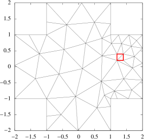
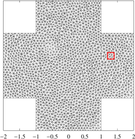
Figure 1: Cross domain, computational domain $\Omega$ an initial mesh and the domain of interest $\Omega_{J}$ (small red square) (left), the finer uniform mesh (center) and the adaptively refined mesh (right).

4.2 Approximation of the quantity of interest

For each of the four corresponding discrete problems (uniform/adapted mesh and $P_{2}$/$P_{4}$ approximations) we carried out the solution of the corresponding algebraic systems (38) by the BiCG method from Algorithm 1. Since the method has tendency to stagnate after some number of iterations, we restarted the computations once after 400 BiCG iterations. Table 1 shows the limit values of $J({u_{h}})=\mbox{\boldmath$c$\unboldmath}^{{\mkern-1.5mu\mathsf{T}}}\mathbb{A}^{-1}\mbox{\boldmath$b$\unboldmath}$.

mesh uniform	$P_{2}$	${\mathrm{DoF}}=$ 22452	0.4071783143507507
mesh uniform	$P_{4}$	${\mathrm{DoF}}=$ 56130	0.4075262691478035
mesh adapted	$P_{2}$	${\mathrm{DoF}}=$ 24000	0.4076152998044911
mesh adapted	$P_{4}$	${\mathrm{DoF}}=$ 60000	0.4076169203362077

Table 1: Cross domain, computation on fixed meshes, the limit values of the quanitity of interest $J({u_{h}})=\mbox{\boldmath$c$\unboldmath}^{{\mkern-1.5mu\mathsf{T}}}\mathbb{A}^{-1}\mbox{\boldmath$b$\unboldmath}$ after three restarts on two meshes (uniform/adapted) and $P_{2}$ and $P_{4}$ approximations.

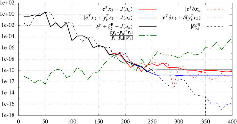
Figure 5: Convergence of the algebraic error and its estimates for the BiCG solver, case adapted mesh, $P_{4}$ approximation, the errors of the approximation of the quantity of interest (P1), (P2), (P3) (solid lines), their approximation (E1), (E2), (E3) (dashed lines) and the lost of the orthogonality (dotted-dashed line).

Figures 2 – 5 show the results obtained within the first 400 BiCG iterations, namely

• the convergence of the errors three types of the approximation of the quantity of interest $J({u_{h}})=\mbox{\boldmath$c$\unboldmath}^{{\mkern-1.5mu\mathsf{T}}}\mathbb{A}^{-1}\mbox{\boldmath$b$\unboldmath}$, namely

  • (P1): $|\mbox{\boldmath$c$\unboldmath}^{{\mkern-1.5mu\mathsf{T}}}\mbox{\boldmath$x$\unboldmath}_{k}-J({u_{h}})|$ following from (48),

  • (P2): $|\mbox{\boldmath$c$\unboldmath}^{{\mkern-1.5mu\mathsf{T}}}\mbox{\boldmath$x$\unboldmath}_{k}+\mbox{\boldmath$y$\unboldmath}_{k}^{{\mkern-1.5mu\mathsf{T}}}\mbox{\boldmath$r$\unboldmath}_{k}-J({u_{h}})|$ following from (50),

  • (P3): $|{\xi}^{\mathrm{p}}+{\xi}_{k}^{B}-J({u_{h}})|$ following from (60),

  where $J({u_{h}})$ is the limit value from Table 1 and $|\cdot|$ is the absolute value,

• the convergence of the values of three different estimations of the error of the approximation of the quanitity of interest, namely

  • (E1): $|\mbox{\boldmath$c$\unboldmath}^{{\mkern-1.5mu\mathsf{T}}}\delta\mbox{\boldmath$x$\unboldmath}_{k}|$ following from (65),

  • (E2): $|\mbox{\boldmath$c$\unboldmath}^{{\mkern-1.5mu\mathsf{T}}}\delta\mbox{\boldmath$x$\unboldmath}_{k}+\delta(\mbox{\boldmath$y$\unboldmath}_{k}^{{\mkern-1.5mu\mathsf{T}}}\mbox{\boldmath$r$\unboldmath}_{k})|$ following from (67),

  • (E3): $|\delta{\xi}^{\mathrm{B}}_{k}|$ following from (69),

  where symbol $\delta$ denotes the difference between $k$-th and $(k+\nu)$-th iterations, i.e, $\delta\mbox{\boldmath$x$\unboldmath}_{k}=\mbox{\boldmath$x$\unboldmath}_{k+\nu}-\mbox{\boldmath$x$\unboldmath}_{k}$, $\delta(\mbox{\boldmath$y$\unboldmath}_{k}^{{\mkern-1.5mu\mathsf{T}}}\mbox{\boldmath$r$\unboldmath}_{k})=\mbox{\boldmath$y$\unboldmath}_{k+\nu}^{{\mkern-1.5mu\mathsf{T}}}\mbox{\boldmath$r$\unboldmath}_{k+\nu}-\mbox{\boldmath$y$\unboldmath}_{k}^{{\mkern-1.5mu\mathsf{T}}}\mbox{\boldmath$r$\unboldmath}_{k}$, $\delta{\xi}^{\mathrm{B}}_{k}={\xi}^{\mathrm{B}}_{k+\nu}-{\xi}^{\mathrm{B}}_{k}$, in the experiments, we put uniquely $\nu=10$,

• the quantity

  • $\frac{|(\mbox{\boldmath$y$\unboldmath}_{k}-\mbox{\boldmath$y$\unboldmath}_{0})^{\mkern-1.5mu\mathsf{T}}\mbox{\boldmath$r$\unboldmath}_{k}|}{\|\mbox{\boldmath$y$\unboldmath}_{k}-\mbox{\boldmath$y$\unboldmath}_{0}\|\,\|\mbox{\boldmath$r$\unboldmath}_{k}\|}$ measuring the lost of the orthogonality, cf. (56).

We observe the following.

1. The errors of all approximations of the quantity of interest (solid lines) decrease until they reach some level of accuracy. After reaching this level they stagnate. This is in agreement with the results in Gr1997 where its is showen that the residual norms $\|\mbox{\boldmath$r$\unboldmath}_{k}\|$ of the Krylov subspace methods like BiCG, reach (if they converge) the level of accuracy close to $\varepsilon\|A\|\Theta$ where $\varepsilon$ is the machine precision and $\Theta=\max\{\|\mbox{\boldmath$x$\unboldmath}_{k}\|\}$ (unpreconditioned case).

2. All approximation of the quantity of interest (P1) – (P3) (solid lines) have almost identical convergence as long as the lost of orthogonality (56) is small (dotted-dashed line). When the lost of orthogonality starts to play more important role the values of the approximation of the quantity of interest slightly differ.

3. Similarly, all the estimations of the error of approximations (E1) – (E3) (dashed lines) have almost identical convergence as long as the lost of orthogonality is small. If the evaluations of the quantity of interests start to stagnate the estimates (E1) – (E3) underestimate the error. This process is the slowest for (E1) but it is presented too.

From these observations, we conclude that any error estimate (E1) – (E3) can be used for the stopping criterion. They underestimate the error only when the computational process stagnates and then it make no sense to proceed with next iterative steps. Based on the argumentation in Section 3.4, criteria (E2) and (E3) are less sensitive to the lost of orthogonality. Finally, criterion (E3) is cheaper to evaluate than (E2) but, in our case, it does not play any essential role in the whole computational process.

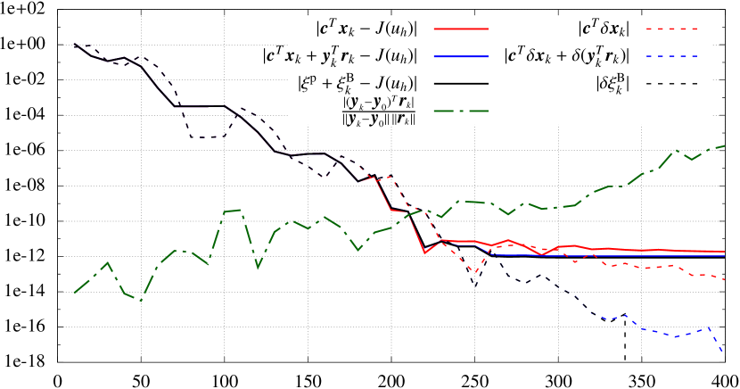
Figure 2: Convergence of the algebraic error and its estimates for the BiCG solver, case uniform mesh, $P_{2}$ approximation, the errors of the approximation of the quantity of interest (P1), (P2), (P3) (solid lines), their approximation (E1), (E2), (E3) (dashed lines) and the lost of the orthogonality (dotted-dashed line).

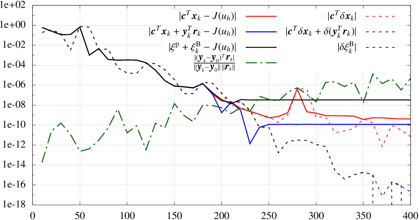
Figure 3: Convergence of the algebraic error and its estimates for the BiCG solver, case uniform mesh, $P_{4}$ approximation, the errors of the approximation of the quantity of interest (P1), (P2), (P3) (solid lines), their approximation (E1), (E2), (E3) (dashed lines) and the lost of the orthogonality (dotted-dashed line).

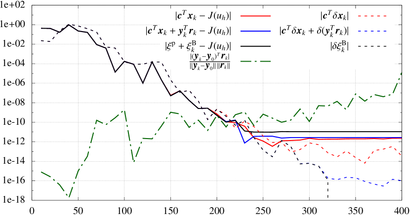
Figure 4: Convergence of the algebraic error and its estimates for the BiCG solver, case adapted mesh, $P_{2}$ approximation, the errors of the approximation of the quantity of interest (P1), (P2), (P3) (solid lines), their approximation (E1), (E2), (E3) (dashed lines) and the lost of the orthogonality (dotted-dashed line).

5 Adaptive mesh refinement and algebraic stopping criteria

The goal of the numerical solution of (1) is to obtain a numerical approximation ${\tilde{u}_{h}}$ such that (cf. (29))

$$|J({u})-J({\tilde{u}_{h}})|\approx\eta_{\mathrm{S},k}+\eta_{\mathrm{A},k}\leq{{\omega}},$$ (71)

where ${{\omega}}>0$ is the given tolerance. The adaptive mesh refinement allows to reduce the computation costs necessary to achieve (71).

5.1 Mesh adaptation algorithm

The idea of the mesh adaptive algorithm is to start on an initial coarse mesh ${\mathscr{T}}_{h,0}$ (dimension of the corresponding space $V_{h,0}$ is small). Then for $m=0,1,\dots$, we discretize and solve both primal and dual problem on $V_{h,m}$ and estimate the error of the quantity of interest. If the estimate does not fulfil (71) then we adapt the mesh and create a new one ${\mathscr{T}}_{h,{m+1}}$ and proceed with the computation. Algorithm 2 shows the abstract form of the adaptive mesh refinement algorithm. It means that we obtain the approximations of the primal and dual solutions $u_{h,m}^{k}\in V_{h,m}$ and $z_{h,m}^{k}\in V_{h,m}$, where subscript $m$-th corresponds to the level of mesh adaptation and subscript $k$-th corresponds to the algebraic iteration.

Algorithm 2 Mesh adaptation process

1:  let ${\mathscr{T}}_{h,0}$ be the initial (coarse) mesh

2:  let $V_{h,0}$ be the corresponding finite element space

3:  for $m=0,1,\dots$ do

4:     set the algebraic problems (38) corresponding to the discretization of (1) and (2), respectively, on $V_{h,m}$, i.e.,

$$\mathbb{A}_{m}\mbox{\boldmath$x$\unboldmath}_{m}=\mbox{\boldmath$b$\unboldmath}_{m}\qquad\mbox{and}\qquad\mathbb{A}_{m}^{{\mkern-1.5mu\mathsf{T}}}\mbox{\boldmath$y$\unboldmath}_{m}=\mbox{\boldmath$c$\unboldmath}_{m},$$ (72)

where $\mbox{\boldmath$b$\unboldmath}_{m},\mbox{\boldmath$c$\unboldmath}_{m}\in{\mathbb{R}}^{N_{m}}$, $\mathbb{A}_{m}\in{\mathbb{R}}^{N_{m}\times N_{m}}$, $\dim V_{h,m}=N_{m}$,

5:     apply an iterative algebraic solver

6:     for $k=0,1,\dots$ do

7:        evaluate $\mbox{\boldmath$x$\unboldmath}_{m,k}$ and $\mbox{\boldmath$y$\unboldmath}_{m,k}$ approximations of (72)

8:        if  algebraic stopping criterion is achieved then

9:           EXIT

10:        end if

11:     end for

12:     define $u_{h,m}^{k},z_{h,m}^{k}\in V_{h,m}$ corresponding to $\mbox{\boldmath$x$\unboldmath}_{m,k}$ and $\mbox{\boldmath$y$\unboldmath}_{m,k}$ (the outputs of Algorithm 1)

13:     define higher-order reconstructions $u_{h,m}^{+}={\mathscr{R}}(u_{h,m}^{k})$ and $z_{h,m}^{+}={\mathscr{R}}(z_{h,m}^{k})$ using (27)

14:     employing (28)–(30), evaluate the goal oriented error estimates

$$\eta_{m,k}:=\eta_{\mathrm{S},m,k}+\eta_{\mathrm{A},m,k},\qquad\eta_{m,k}^{*}:=\eta_{\mathrm{S},m,k}^{*}+\eta_{\mathrm{A},m,k}^{*}$$ (73)

where

$$\eta_{\mathrm{S},m,k}:=r_{h}(u_{h,m}^{k})(z_{h,m}^{+}-z_{h,m}^{k}), \eta_{\mathrm{A},m,k}:=r_{h}(u_{h,m}^{k})(z_{h,m}^{k}),$$ (74)

$$\eta_{\mathrm{S},m,k}^{*}:=r_{h}^{*}(z_{h,m}^{k})(u_{h,m}^{+}-u_{h,m}^{k}), \eta_{\mathrm{A},m,k}^{*}:=r_{h}^{*}(z_{h,m}^{k})(u_{h,m}^{k}),$$

15:     if $\eta_{m,k}\leq{{\omega}}$ and $\eta_{m,k}^{*}\leq{{\omega}}$ then

16:         STOP the computational process with the output quantity $J(u_{h,m}^{k})$ and its estimate $\eta_{m,k}$,

17:     else

18:        based on a localization of $\eta_{m,k}$, adapt the mesh, i.e., modify the size and/or the shape of elements and possibly also the polynomial approximation degrees, the new mesh is ${\mathscr{T}}_{h,{m+1}}$ and the corresponding space $V_{h,{m+1}}$,

19:     end if

20:  end for

Step 18 of Algorithm 2 (mesh adaptation) depends on the used discretization method and the refinement technique. In order to demonstrate the robustness of the presented stopping criteria, we use the anisotropic $hp$-mesh adaptation approach from ESCO-18 , which generate anisotropic meshes (consisting of possibly thin and long triangular elements) and varying polynomial approximation degree.

The crucial aspect is the algebraic stopping criterion in step 8 of Algorithm 2 which is discussed in the next section.

5.2 Standard stopping criteria for the solution of algebraic systems

We focus on the algebraic stopping criterion in Step 8 of Algorithm 2. Obviously, too strong criterion leads to many algebraic iterations without a gain of accuracy. On the other hand, the weak criterion leads to an under-solving of (72) which affect the mesh adaptation process. Typically too many mesh elements are generated.

Often the residual stopping criteria for (72) are used, i.e.,

$$\|\mbox{\boldmath$r$\unboldmath}_{m,k}\|:=\|\mbox{\boldmath$b$\unboldmath}_{m}-\mathbb{A}_{m}\mbox{\boldmath$x$\unboldmath}_{m,k}\|\leq{\omega_{\mathrm{{A}}}},\qquad\|\mbox{\boldmath$s$\unboldmath}_{m,k}\|:=\|\mbox{\boldmath$c$\unboldmath}_{m}-\mathbb{A}_{m}^{{\mkern-1.5mu\mathsf{T}}}\mbox{\boldmath$y$\unboldmath}_{m,k}\|\leq{\omega_{\mathrm{{A}}}},$$ (75)

or their preconditioned variant

$$\|\mathbb{P}^{-1}(\mbox{\boldmath$b$\unboldmath}_{m}-\mathbb{A}_{m}\mbox{\boldmath$x$\unboldmath}_{m,k})\|\leq{\omega_{\mathrm{{A}}}},\qquad\|\mathbb{P}^{-{\mkern-1.5mu\mathsf{T}}}(\mbox{\boldmath$c$\unboldmath}_{m}-\mathbb{A}_{m}^{{\mkern-1.5mu\mathsf{T}}}\mbox{\boldmath$y$\unboldmath}_{m,k})\|\leq{\omega_{\mathrm{{A}}}},$$ (76)

where $\mathbb{P}$ represents a suitable preconditioner, cf. (57). This criterion is easy to evaluate but the choice of the suitable tolerance ${\omega_{\mathrm{{A}}}}>0$ is difficult since this criterion has no relation to the discretization error.

This drawback was eliminated in Meidner2009Goal by the following stopping criterion

$$\eta_{\mathrm{A},m,k}\leq{c_{\mathrm{A}}}\eta_{\mathrm{S},m,k},\qquad\eta_{\mathrm{A},m,k}^{*}\leq{c_{\mathrm{A}}}\eta_{\mathrm{S},m,k}^{*},$$ (77)

where the primal/dual estimates of the algebraic/discretization errors are defined by (74) and ${c_{\mathrm{A}}}\in(0,1)$ is a suitable constant. This means that Steps 12-14 of Algorithm 2 are moved inside the inner loop (after Step 7). We call this criterion as algebraic goal-oriented stopping criterion.

The conditions (77) allow to control the size of the algebraic error. However, a strong drawback of (77) are to computational costs. Whereas the evaluation of $\eta_{\mathrm{A},m,k}$ and $\eta_{\mathrm{A},m,k}^{*}$ is cheap, the computation of $\eta_{\mathrm{S},m,k}$ and $\eta_{\mathrm{S},m,k}^{*}$ is much more expensive namely due to the necessity to perform the higher-order reconstructions $u_{h,m}^{+}$ and $z_{h,m}^{+}$ (Step 13). The computational costs can be reduced by testing (77) only after some number of iterations, e.g., after 1-3 restarts of iterative solver. In Meidner2009Goal , the first condition of (77) was tested after the performing of one cycle of multigrid method.

5.3 New stopping criteria for the solution of algebraic systems

In Section 2.6, we introduced two alternative formula for the decomposition of the computational errors into the discretization and algebraic parts, namely using (31) and (32), we have

$$J({u}-u_{h,m}^{k}) =r_{h}(u_{h,m}^{k})({z}-z_{h,m}^{k})+r_{h}(u_{h,m}^{k})(z_{h,m}^{k}) ={e_{\mathrm{S},m,k}}+{e_{\mathrm{A},m,k}},$$ (78)

$$J({u}-u_{h,m}^{k}) =J({u}-u_{h,m})+J(u_{h,m}-u_{h,m}^{k}) =\zeta_{\mathrm{S},m,k}+\zeta_{\mathrm{A},m,k}.$$

Similarly, (26) and (36) imply the dual counterpart

$$\ell_{h}({z}-z_{h,m}^{k}) =r_{h}^{*}(z_{h,m}^{k})({u}-u_{h,m}^{k})+r_{h}^{*}(z_{h,m}^{k})(u_{h,m}^{k}) ={e_{\mathrm{S},m,k}^{*}}+{e_{\mathrm{A},m,k}^{*}},$$ (79)

$$\ell_{h}({z}-z_{h,m}^{k}) =\ell_{h}({z}-z_{h,m})+\ell_{h}(z_{h,m}-z_{h,m}^{k}) =\zeta_{\mathrm{S},m,k}^{*}+\zeta_{\mathrm{A},m,k}^{*}.$$

The discussion presented therein shows that both quantities ${e_{\mathrm{A},m,k}}\not=\zeta_{\mathrm{A},m,k}$ corresponds to the algebraic error of the primal problem and similarly, ${e_{\mathrm{A},m,k}^{*}}\not=\zeta_{\mathrm{A},m,k}^{*}$ corresponds to the algebraic error of the dual one.

In Section 3.4, we presented several techniques estimating the quantities $\zeta_{\mathrm{A},m,k}$ and $\zeta_{\mathrm{A},m,k}^{*}$ by techniques (E1) – (E3). On the other hand, quantities ${e_{\mathrm{A},m,k}}$ and ${e_{\mathrm{A},m,k}^{*}}$ are available during the BiCG iterative method since

$${e_{\mathrm{A},m,k}} =\eta_{\mathrm{A},m,k}=r_{h}(u_{h,m}^{k})(z_{h,m}^{k})=\mbox{\boldmath$y$\unboldmath}_{k}^{{\mkern-1.5mu\mathsf{T}}}\mbox{\boldmath$r$\unboldmath}_{k},$$ (80)

$${e_{\mathrm{A},m,k}^{*}} =\eta_{\mathrm{A},m,k}^{*}=r_{h}^{*}(z_{h,m}^{k})(u_{h,m}^{k})=\mbox{\boldmath$s$\unboldmath}_{k}^{{\mkern-1.5mu\mathsf{T}}}\mbox{\boldmath$x$\unboldmath}_{k},$$

cf. (30) and (46).

Figure 6 shows a typical dependence of these quantities w.r.t. the number of BiCG iterations during mesh adaptation process by Algorithm 2 for $m=0,\dots,5$. In the top figure, we plot the total error $J({u}-u_{h,m}^{k})$, the exact algebraic error $\zeta_{\mathrm{A},m,k}=J(u_{h,m}-u_{h,m}^{k})$, the algebraic error ${e_{\mathrm{A},m,k}}=\mbox{\boldmath$s$\unboldmath}_{k}^{{\mkern-1.5mu\mathsf{T}}}\mbox{\boldmath$x$\unboldmath}_{k}$ and the estimates (E1) and (E2) of $\zeta_{\mathrm{A},m,k}$ from Section 3.4. The bottom figure shows the dual counterparts. Estimate (E3) gives the same graphs as (E2) so we do not show it.

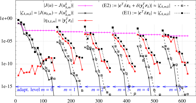
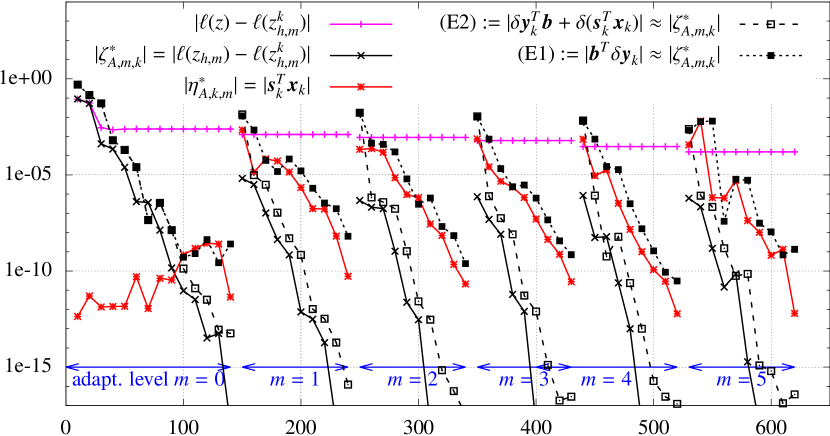
Figure 6: Typical example of the adaptive computations for mesh adaptation steps $m=0,\dots,5$, dependence of primal (top) and dual (bottom) quantities w.r.t. the number of BiCG steps.

We observe that estimate (E2) approximates $\zeta_{\mathrm{A},m,k}$ similarly as (E1) for the moderate values of accuracy but much better on the level close to the machine accuracy. This is in agreement with theoretical considerations in Section 3.4, but this effect is not observed on the initial mesh ($m=0$) when we do not have a good initial approximation. Further, both algebraic error representations converge but with different speed. Whereas on the initial mesh we have $\eta_{\mathrm{A},0,k}\ll\zeta_{\mathrm{A},0,k}$ for $k\leq 100$, starting from $m=1$ we observe $\eta_{\mathrm{A},m,k}\gg\zeta_{\mathrm{A},m,k}$. Similar behaviour is observed for the dual quantities.

Based on this observation, we consider both pairs of quantities $(\eta_{\mathrm{A},m,k},\zeta_{\mathrm{A},m,k})$ and $(\eta_{\mathrm{A},m,k}^{*},\zeta_{\mathrm{A},m,k}^{*})$ for the definition of the stopping criterion, namely, we evaluate the quantities

$$\sigma_{\mathrm{A},m,k}:= |\delta{\xi}^{\mathrm{B}}_{k}|+|\eta_{\mathrm{A},m,k}|=|{\xi}^{\mathrm{B}}_{k+\nu}-{\xi}^{\mathrm{B}}_{k}|+|\mbox{\boldmath$y$\unboldmath}_{k,m}^{{\mkern-1.5mu\mathsf{T}}}\mbox{\boldmath$r$\unboldmath}_{k,m}|,$$ (81)

$$\sigma_{\mathrm{A},m,k}^{*}:= |\delta{\xi}^{\mathrm{B}}_{k}|+|\eta_{\mathrm{A},m,k}^{*}|=|{\xi}^{\mathrm{B}}_{k+\nu}-{\xi}^{\mathrm{B}}_{k}|+|\mbox{\boldmath$s$\unboldmath}_{k,m}^{{\mkern-1.5mu\mathsf{T}}}\mbox{\boldmath$x$\unboldmath}_{k,m}|,$$

corresponding to the $k$-iteration of the BiCG Algorithm 1 on $m$-level of mesh adaptation. Let us recall that quantities $\sigma_{\mathrm{A},m,k}$ and $\sigma_{\mathrm{A},m,k}^{*}$ are available during the whole BiCG iterative process with negligible computational costs.

Now we define a new algebraic stopping criterion (called hereafter $\sigma$-stopping criterion) for Algorithm 2 (Step 8) by

$$\sigma_{\mathrm{A},m,k}\leq{c_{\mathrm{A}}}{{\omega}}\qquad\mbox{and}\qquad\sigma_{\mathrm{A},m,k}^{*}\leq{c_{\mathrm{A}}}{{\omega}},$$ (82)

where ${{\omega}}>0$ is the (global) tolerance from (71) and ${c_{\mathrm{A}}}\in(0,1)$ is a suitable constant. In contrary to the stopping criterion (77), the proposed one (82) does not take into account the (estimate of) the discretization error and consequently the strong advantage of (82) is that its evaluation is very fast.

We can summarized the idea of the original stopping criterion (77) as follows: “algebraic system is solved as long the algebraic error is ${c_{\mathrm{A}}}$-times smaller than the discretization error”. On the other hand, the idea of the new stopping criterion (82) is the following: “algebraic system is solved as long the algebraic error is ${c_{\mathrm{A}}}$-times smaller than the prescribed tolerance for the discretization error”.

The stopping criterion (82) does not look to much efficient since for starting levels of mesh adaptation, when $\eta_{\mathrm{S},m,k}\gg{{\omega}}$ and $\eta_{\mathrm{S},m,k}^{*}\gg{{\omega}}$, the iterative solver is stopped when the algebraic error is much lower than the discretization one. It is true but on the other hand performing of additional several teens of BiCG iterations is typically faster than the evaluation of $\eta_{\mathrm{S},m,k}$ and $\eta_{\mathrm{S},m,k}^{*}$. Moreover, approximate solutions computed using BiCG on starting levels serve as good initial approximations for BiCG on higher levels, which improve then the solving process significantly.

6 Numerical experiments on adaptively refined meshes

We demonstrate the computational performance of the stopping criteria from Sections 5.2 and 5.3. We consider two numerical examples, the first one is the elliptic problem on the “cross” domain described in Section 4.1 and the second one is a convection-dominated problem having some anisotropic features, it is defined in Section 6.1. Both problems are discretized again by the SIPG method and the meshes are adapted by the technique from ESCO-18 . Each mesh ${\mathscr{T}}_{h,m}$ is generated from the computed primal and dual solutions on the previous one. These solutions are interpolated to the actual mesh, hence we have relatively very good initial approximations $\mbox{\boldmath$x$\unboldmath}_{m,0}$ and $\mbox{\boldmath$y$\unboldmath}_{m,0}$ for the solution of (72).

6.1 Convection-dominated problem

The second example is taken from FormaggiaPerotto04 , see also ESCO-18 ; CarpioPrietoBermejo_SISC13 . We solve the convection-diffusion equation

$$-\varepsilon\Delta u+\nabla\cdot(\mbox{\boldmath$b$\unboldmath}\,u) =0\qquad\text{in }\Omega:=[0,4]\times[0,4]\setminus[0,2]\times[0,2],$$ (83)

where $\varepsilon=10^{-3}$, the convection field $\mbox{\boldmath$b$\unboldmath}=(x_{2},-x_{1})$ and $\nabla\cdot$ is the divergence operator. We prescribe the Dirichlet and Neumann boundary conditions

$$u=1 \quad\mbox{ on }\{x_{1}=0\},$$ (84)

$$\nabla u\cdot\mbox{\boldmath$n$\unboldmath}=0 \quad\mbox{ on }\Gamma_{1}:=\{{\Gamma};x_{1}=4\}\cup\Gamma_{2}:=\{{\Gamma};x_{2}=0\},$$

$$u=0 \quad\mbox{ elsewhere}.$$

The solution $u$ exhibits boundary layers as well as two circular-shaped internal layers. We consider the functional $J(u)=\int_{\Gamma_{1}}\mbox{\boldmath$b$\unboldmath}\cdot\mbox{\boldmath$n$\unboldmath}\,u\,{\rm d}S$ with the reference value $J(u)=0.07408122\pm 10^{-8}$.

6.2 Comparison of the stopping criteria

In order to demonstrate the robustness of the proposed stopping criteria, we solve the elliptic problem (70) and the convection-diffusion problem (83) by the mesh adaptation Algorithm 2. For both problems, we employ the anisotropic $h$-mesh adaptation using $P_{3}$ approximation and anisotropic $hp$-mesh adaptation, for details we refer to ESCO-18 . In order to observe the effect with not sufficiently resolved algebraic systems (72), we stop the adaptation process when

$$\frac{1}{2}\left(\eta_{\mathrm{S},m,k}+\eta_{\mathrm{S},m,k}^{*}\right)\leq{{\omega}},$$ (85)

where $\eta_{\mathrm{S},m,k}$ and $\eta_{\mathrm{S},m,k}^{*}$ are given by (74) and we put ${{\omega}}=10^{-8}$ for the elliptic problem (70) and ${{\omega}}=10^{-10}$ for the convection-diffusion problem (83).

We test Algorithm 2 with the following iterative solvers and the stopping criteria.

1. GMRES with preconditioned residual stopping criterion (76) with tolerances ${\omega_{\mathrm{{A}}}}=10^{-9}$, $10^{-6}$ and $10^{-3}$,

2. BiCG with preconditioned residual stopping criterion (76) with tolerances ${\omega_{\mathrm{{A}}}}=10^{-9}$, $10^{-6}$ and $10^{-3}$,

3. GMRES with algebraic goal-oriented stopping criterion (77) with tolerances ${c_{\mathrm{A}}}=10^{-2}$, $10^{-1}$ and $10^{0}$,

4. BiCG with algebraic goal-oriented stopping criterion (77) with tolerances ${c_{\mathrm{A}}}=10^{-2}$, $10^{-1}$ and $10^{0}$,

5. BiCG with $\sigma$-stopping criterion (82) with tolerances ${c_{\mathrm{A}}}=10^{-2}$, $10^{-1}$ and $10^{0}$.

For all solvers we use the block-ILU(0) preconditioner which is suitable for discontinuous Galerkin method, cf. lin_algeb . For GMRES, we solve first the primal problem and then the dual problem, for BiCG, both problems are solved at once, of course. Moreover, GMRES is restarted always after 45 iterations. In case (c), the stopping criterion (77) is tested after one restart of GMRES for the primal as well as the dual problems. In case (d), the stopping criterion (77) is tested after 100 BiCG iterations.

The results are presented in Tables 2 – 5, where we show the number of degrees of freedom ${\mathrm{DoF}}$ on the last mesh, the total error $J({u}-u_{h,m}^{k})$, the final estimator of the discretization and algebraic errors $\eta_{\mathrm{S},m,k}$ and $\eta_{\mathrm{A},m,k}$, respectively and their sum $\eta_{m,k}$. Moreover, these tables contains the total number of (GMRES or BiCG) iterations on all mesh levels $m=0,1,\dots$ (iters) and the total computational time in seconds. If $\eta_{\mathrm{A},m,k}\geq\eta_{\mathrm{S},m,k}$ then the line ends with the character ’!’.

We remind that the error estimator $\eta_{m,k}$ does not give the upper bound, see Remark 1. There are small differences for each of four examples but we can state the following observations.

• the use of the preconditioned residual stopping criterion (76) for GMRES as well as BiCG with too large ${\omega_{\mathrm{{A}}}}$ leads to the dominance of the algebraic error and consequently $J(u-u_{h,m}^{k})$ and $\eta_{m,k}$ are much larger then the tolerance ${{\omega}}$ from (71) and (85), cf. (a) and (b),

• GMRES requires more iterations then BiCG since the primal and dual problems are solver separately, therefore BiCG is faster, compare (a) vs. (b) and (c) vs. (d),

• the goal-oriented stopping criterion (77) allows to control the algebraic (and therefore also the total) error as expected for GMRES and BiCG, see (c) and (d),

• the $\sigma$-stopping criterion (82) works efficiently, the algebraic error estimator $\eta_{\mathrm{A},m,k}$ is smaller than the discretization one $\eta_{\mathrm{S},m,k}$, the computational time is substantially reduced in comparison with the goal-oriented criterion (77) since the higher-order reconstructions is performed less frequently, see the last paragraph in Section 5.2.

${\omega_{\mathrm{{A}}}}$ or ${c_{\mathrm{A}}}$	${\mathrm{DoF}}$	$J({u}-u_{h,m}^{k})$	$\eta_{\mathrm{S},m,k}$	$\eta_{\mathrm{A},m,k}$	$\eta_{m,k}$	iters	time(s)
(a)    GMRES preconditioned residual stopping criterion
1.E-09	92680	2.33E-08	6.72E-09	8.80E-11	6.81E-09	8301	480.5
1.E-06	93120	9.76E-08	7.47E-09	5.24E-08	5.99E-08	3274	235.0	!
1.E-03	94680	1.27E-04	7.36E-09	9.25E-05	9.25E-05	806	144.2	!
(b)    BiCG preconditioned residual stopping criterion
1.E-09	92680	2.32E-08	6.72E-09	6.26E-13	6.72E-09	3150	341.8
1.E-06	90700	2.67E-08	7.96E-09	5.07E-11	8.01E-09	2170	258.6
1.E-03	90050	4.80E-07	7.94E-09	2.54E-07	2.62E-07	900	160.0	!
(c)    GMRES algebraic goal-oriented stopping criterion
1.E-02	91770	3.19E-08	9.46E-09	3.05E-11	9.49E-09	7560	867.2
1.E-01	95230	2.61E-08	6.74E-09	1.77E-10	6.92E-09	6480	768.5
1.E+00	93440	3.06E-08	7.09E-09	2.12E-09	9.21E-09	4860	553.7
(d)    BiCG algebraic goal-oriented stopping criterion
1.E-02	94170	2.56E-08	6.71E-09	1.19E-11	6.72E-09	3400	677.9
1.E-01	90800	2.69E-08	7.83E-09	5.76E-10	8.40E-09	2700	534.8
1.E+00	91680	3.67E-08	9.34E-09	2.29E-09	1.16E-08	2200	374.3
(e)    BiCG $\zeta$-stopping criterion
1.E-02	89760	8.20E-06	8.42E-09	6.13E-06	6.13E-06	750	233.3	!
1.E-01	94320	1.74E-05	6.07E-09	1.16E-05	1.16E-05	610	179.5	!
1.E+00	91660	5.77E-05	8.22E-09	4.35E-05	4.35E-05	430	160.1	!
(f)    BiCG $\eta$-stopping criterion
1.E-02	122070	1.05E-08	3.14E-09	2.84E-11	3.17E-09	2950	479.7
1.E-01	121760	8.78E-09	2.45E-09	7.33E-10	3.19E-09	2550	399.7
1.E+00	121620	1.42E-08	3.16E-09	1.82E-09	4.99E-09	2270	411.3
(g)    BiCG $\sigma$-stopping criterion
1.E-02	93560	2.59E-08	6.90E-09	2.41E-11	6.93E-09	2340	277.4
1.E-01	90730	2.94E-08	7.68E-09	2.77E-10	7.96E-09	1890	229.7
1.E+00	91110	3.40E-08	7.30E-09	5.15E-09	1.25E-08	1730	226.5

Table 2: Elliptic problem (70), $h$-mesh adaptation with $P_{3}$ approximation, comparison of solvers and stopping criteria, ${{\omega}}=10^{-8}$.

${\omega_{\mathrm{{A}}}}$ or ${c_{\mathrm{A}}}$	${\mathrm{DoF}}$	$J({u}-u_{h,m}^{k})$	$\eta_{\mathrm{S},m,k}$	$\eta_{\mathrm{A},m,k}$	$\eta_{m,k}$	iters	time(s)
(a)    GMRES preconditioned residual stopping criterion
1.E-09	22390	3.15E-08	6.02E-09	9.33E-12	6.03E-09	4810	183.1
1.E-06	24160	3.84E-08	5.17E-09	2.66E-08	3.17E-08	2627	121.4	!
1.E-03	23845	2.90E-05	8.24E-09	1.83E-05	1.83E-05	602	87.8	!
(b)    BiCG preconditioned residual stopping criterion
1.E-09	23520	3.38E-08	7.73E-09	7.46E-14	7.73E-09	2360	152.0
1.E-06	25656	2.07E-08	3.80E-09	6.73E-11	3.87E-09	1700	138.4
1.E-03	25364	9.51E-08	7.03E-09	3.15E-08	3.85E-08	970	114.5	!
(c)    GMRES algebraic goal-oriented stopping criterion
1.E-02	24575	2.58E-08	5.00E-09	6.44E-13	5.00E-09	3753	200.7
1.E-01	24468	2.70E-08	5.40E-09	1.09E-10	5.51E-09	3408	167.3
1.E+00	23594	2.75E-08	5.22E-09	1.13E-10	5.34E-09	3228	158.5
(d)    BiCG algebraic goal-oriented stopping criterion
1.E-02	23631	3.12E-08	6.41E-09	3.96E-12	6.41E-09	2100	186.8
1.E-01	23721	2.89E-08	5.14E-09	2.57E-11	5.17E-09	1900	163.6
1.E+00	24006	2.54E-08	4.80E-09	1.23E-12	4.80E-09	1800	162.1
(e)    BiCG $\zeta$-stopping criterion
1.E-02	26627	1.07E-07	5.36E-09	6.34E-08	6.87E-08	830	104.7	!
1.E-01	22219	2.33E-06	9.81E-09	1.24E-06	1.25E-06	600	89.5	!
1.E+00	31772	1.12E-05	8.16E-09	1.24E-05	1.24E-05	520	139.8	!
(f)    BiCG $\eta$-stopping criterion
1.E-02	24783	1.93E-08	3.94E-09	2.42E-11	3.96E-09	1820	168.3
1.E-01	26703	1.41E-08	2.25E-09	1.07E-10	2.35E-09	1680	179.3
1.E+00	26491	2.85E-08	4.84E-09	1.83E-09	6.67E-09	1380	165.6
(g)    BiCG $\sigma$-stopping criterion
1.E-02	24176	2.49E-08	5.07E-09	3.08E-11	5.10E-09	1660	128.0
1.E-01	23064	2.84E-08	5.69E-09	6.39E-10	6.33E-09	1460	117.4
1.E+00	22486	2.84E-08	6.04E-09	9.92E-10	7.04E-09	1300	112.9

Table 3: Elliptic problem (70), $hp$-mesh adaptation, comparison of solvers and stopping criteria, ${{\omega}}=10^{-8}$.

${\omega_{\mathrm{{A}}}}$ or ${c_{\mathrm{A}}}$	${\mathrm{DoF}}$	$J({u}-u_{h,m}^{k})$	$\eta_{\mathrm{S},m,k}$	$\eta_{\mathrm{A},m,k}$	$\eta_{m,k}$	iters	time(s)
(a)    GMRES preconditioned residual stopping criterion
1.E-09	74910	4.36E-12	6.09E-11	2.55E-10	3.15E-10	4862	308.2	!
1.E-06	83960	7.36E-08	3.22E-11	5.29E-08	5.29E-08	2198	240.5	!
1.E-03	70060	4.16E-06	3.25E-11	1.35E-04	1.35E-04	524	163.5	!
(b)    BiCG preconditioned residual stopping criterion
1.E-09	70580	1.07E-10	6.37E-11	6.79E-12	7.05E-11	2920	327.1
1.E-06	78610	4.95E-11	2.80E-11	4.39E-10	4.67E-10	2310	317.1	!
1.E-03	61250	1.37E-08	1.11E-12	2.01E-07	2.01E-07	1100	195.5	!
(c)    GMRES algebraic goal-oriented stopping criterion
1.E-02	52820	3.04E-10	8.52E-11	2.49E-13	8.54E-11	5501	430.6
1.E-01	79990	6.36E-11	5.80E-11	2.99E-12	6.10E-11	6404	679.7
1.E+00	68850	1.50E-10	6.06E-11	1.49E-11	7.56E-11	5324	561.3
(d)    BiCG algebraic goal-oriented stopping criterion
1.E-02	52680	2.46E-10	8.06E-11	4.13E-14	8.07E-11	4180	601.8
1.E-01	73320	1.15E-10	4.66E-11	3.65E-14	4.66E-11	4180	694.3
1.E+00	79170	8.30E-11	3.09E-11	9.52E-12	4.04E-11	4780	1074.4
(e)    BiCG $\zeta$-stopping criterion
1.E-02	76330	3.32E-07	4.21E-11	9.32E-04	9.32E-04	880	208.1	!
1.E-01	106050	4.05E-06	1.41E-11	1.87E-03	1.87E-03	680	214.5	!
1.E+00	63940	3.12E-06	9.97E-11	1.37E-03	1.37E-03	560	152.1	!
(f)    BiCG $\eta$-stopping criterion
1.E-02	72820	8.49E-11	2.74E-11	4.50E-13	2.78E-11	3070	398.8
1.E-01	71380	9.39E-11	3.25E-11	2.54E-12	3.50E-11	2840	433.1
1.E+00	81880	5.95E-11	2.53E-11	1.28E-11	3.81E-11	2630	468.1
(g)    BiCG $\sigma$-stopping criterion
1.E-02	72820	8.49E-11	2.74E-11	4.50E-13	2.78E-11	3070	357.6
1.E-01	71380	9.39E-11	3.25E-11	2.54E-12	3.50E-11	2840	319.4
1.E+00	81880	5.95E-11	2.53E-11	1.28E-11	3.81E-11	2630	338.7

Table 4: Convection-diffusion problem (83), $h$-mesh adaptation with $P_{3}$-approximation, comparison of solvers and stopping criteria, ${{\omega}}=10^{-10}$.

${\omega_{\mathrm{{A}}}}$ or ${c_{\mathrm{A}}}$	${\mathrm{DoF}}$	$J({u}-u_{h,m}^{k})$	$\eta_{\mathrm{S},m,k}$	$\eta_{\mathrm{A},m,k}$	$\eta_{m,k}$	iters	time(s)
(a)    GMRES preconditioned residual stopping criterion
1.E-09	15852	5.93E-10	4.54E-13	6.76E-11	6.81E-11	2909	124.0	!
1.E-06	18233	1.46E-09	6.76E-11	3.33E-08	3.33E-08	2006	151.9	!
1.E-03	20422	3.08E-06	4.89E-11	9.65E-06	9.65E-06	590	119.0	!
(b)    BiCG preconditioned residual stopping criterion
1.E-09	19905	6.20E-11	4.33E-11	7.96E-12	5.13E-11	1980	178.0
1.E-06	18408	2.26E-11	5.13E-11	1.39E-10	1.91E-10	1550	163.6	!
1.E-03	23431	2.56E-08	2.50E-11	1.49E-06	1.49E-06	820	146.0	!
(c)    GMRES algebraic goal-oriented stopping criterion
1.E-02	19323	5.46E-11	3.29E-12	5.32E-15	3.29E-12	4690	263.9
1.E-01	17504	1.81E-10	9.99E-11	1.66E-14	9.99E-11	3876	221.3
1.E+00	24723	1.25E-11	4.92E-11	4.30E-13	4.97E-11	4236	282.6
(d)    BiCG algebraic goal-oriented stopping criterion
1.E-02	18689	8.64E-11	5.22E-12	2.18E-14	5.25E-12	3870	383.5
1.E-01	18668	9.03E-11	2.44E-11	3.54E-13	2.48E-11	2670	257.1
1.E+00	17240	2.64E-10	5.22E-11	1.61E-12	5.38E-11	2270	203.2
(e)    BiCG $\zeta$-stopping criterion
1.E-02	20038	3.09E-08	1.35E-11	2.25E-05	2.25E-05	880	176.6	!
1.E-01	21598	9.45E-07	5.14E-11	1.99E-04	1.99E-04	780	170.5	!
1.E+00	34233	2.72E-04	6.20E-11	1.40E-03	1.40E-03	810	161.3	!
(f)    BiCG $\eta$-stopping criterion
1.E-02	20146	2.92E-10	2.55E-11	2.89E-13	2.58E-11	1910	181.2
1.E-01	22752	7.32E-11	3.73E-11	1.06E-12	3.83E-11	2090	209.8
1.E+00	22936	4.23E-12	2.00E-11	2.32E-12	2.23E-11	1900	228.2
(g)    BiCG $\sigma$-stopping criterion
1.E-02	20146	2.92E-10	2.55E-11	2.89E-13	2.58E-11	1910	156.3
1.E-01	18757	2.05E-10	1.92E-11	1.32E-12	2.05E-11	1790	148.7
1.E+00	22936	4.23E-12	2.00E-11	2.32E-12	2.23E-11	1900	184.0

Table 5: Convection-diffusion problem (83), $hp$-mesh adaptation, comparison of solvers and stopping criteria, ${{\omega}}=10^{-10}$.

7 Summary of the results and outlook

We developed an efficient technique for the numerical solution of primal and dual algebraic systems arising in the goal-oriented error estimation and mesh adaptation. Both algebraic systems are solved simultaneously by BiCG method which allows to control the algebraic error during the iterative process. The proposed $\sigma$-stopping criterion is cheap for the evaluation and significantly reduce the computational costs. Moreover, it guarantees that the algebraic error estimate bounded by the discretization one.

Further natural step is to extend this approach for the solution of nonlinear partial differential equations. The the dual problem has to be build on a linearization of the primal one. However, employing a Newton-like method for the solution of the discretized primal problem, an approximate solution of the dual problem is available at each Newton step and the technique developed in this paper can be employed. However, it is necessary to balance the linear algebraic errors, the non-linear algebraic errors and the discretization errors. This is the subject of the further work.

Acknowledgements

The authors are thankful to their colleagues from the Charles University, namely M.Kubínová, T. Gergelits and F. Roskovec for a fruitful discussion.

References

- (1) Ainsworth, M., Oden, J.T.: A posteriori error estimation in finite element analysis. Pure and Applied Mathematics (New York). Wiley-Interscience [John Wiley & Sons], New York (2000)
- (2) Ainsworth, M., Rankin, R.: Guaranteed computable bounds on quantities of interest in finite element computations. International Journal for Numerical Methods in Engineering 89(13), 1605–1634 (2012)
- (3) Arioli, M.: A stopping criterion for the conjugate gradient algorithm in a finite element method framework. Numer. Math. 97(1), 1–24 (2004)
- (4) Arioli, M., Liesen, J., Miedlar, A., Strakoš, Z.: Interplay between discretization and algebraic computation in adaptive numerical solution of elliptic PDE problems. GAMM-Mitt. 36(1), 102–129 (2013)
- (5) Balan, A., Woopen, M., May, G.: Adjoint-based -adaptivity on anisotropic meshes for high-order compressible flow simulations. Comput. Fluids 139, 47 – 67 (2016)
- (6) Bangerth, W., Rannacher, R.: Adaptive Finite Element Methods for Differential Equations. Lectures in Mathematics. ETH Zürich. Birkhäuser Verlag (2003)
- (7) Barrett, R., Berry, M., Chan, T.F., et al.: Templates for the solution of linear systems: building blocks for iterative methods. Society for Industrial and Applied Mathematics (SIAM), Philadelphia, PA (1994). DOI 10.1137/1.9781611971538. URL https://doi.org/10.1137/1.9781611971538
- (8) Bartoš, O., Dolejší, V., May, G., , Rangarajan, A., Roskovec, F.: Goal-oriented anisotropic -mesh optimization technique for linear convection-diffusion-reaction problem. Comput. Math. Appl. 78(9), 2973–2993 (2019)
- (9) Becker, R., Rannacher, R.: An optimal control approach to a-posteriori error estimation in finite element methods. Acta Numerica 10, 1–102 (2001)
- (10) Carpio, J., Prieto, J., Bermejo, R.: Anisotropic ”goal-oriented” mesh adaptivity for elliptic problems. SIAM J. Sci. Comput. 35(2), A861–A885 (2013)
- (11) Dolejší, V.: ADGFEM – Adaptive discontinuous Galerkin finite element method, in-house code. Charles University, Prague, Faculty of Mathematics and Physics (2014). http://atrey.karlin.mff.cuni.cz/~dolejsi/adgfem/
- (12) Dolejší, V., Feistauer, M.: Discontinuous Galerkin Method – Analysis and Applications to Compressible Flow. Springer Series in Computational Mathematics 48. Springer, Cham (2015)
- (13) Dolejší, V., Holík, M., Hozman, J.: Efficient solution strategy for the semi-implicit discontinuous Galerkin discretization of the Navier-Stokes equations. J. Comput. Phys. 230, 4176–4200 (2011)
- (14) Dolejší, V., Roskovec, F.: Goal-oriented error estimates including algebraic errors in discontinuous Galerkin discretizations of linear boundary value problems. Appl. Math. 62(6), 579–605 (2017)
- (15) Fidkowski, K., Darmofal, D.: Review of output-based error estimation and mesh adaptation in computational fluid dynamics. AIAA Journal 49(4), 673–694 (2011)
- (16) Fletcher, R.: Conjugate gradient methods for indefinite systems. In: Numerical analysis (Proc 6th Biennial Dundee Conf., Univ. Dundee, Dundee, 1975), pp. 73–89. Lecture Notes in Math., Vol. 506. Springer, Berlin (1976). URL http://www.ams.org/mathscinet-getitem?mr=57#1841
- (17) Formaggia, L., Micheletti, S., Perotto, S.: Anisotropic mesh adaption in computational fluid dynamics: application to the advection-diffusion-reaction and the Stokes problems. Appl. Numer. Math. 51(4), 511–533 (2004)
- (18) Georgoulis, E.H., Hall, E., Houston, P.: Discontinuous Galerkin methods on -anisotropic meshes II: A posteriori error analysis and adaptivity. Appl. Numer. Math. 59(9), 2179–2194 (2009)
- (19) Giles, M., Süli, E.: Adjoint methods for PDEs: a posteriori error analysis and postprocessing by duality. Acta Numerica 11, 145–236 (2002)
- (20) Greenbaum, A.: Estimating the attainable accuracy of recursively computed residual methods. SIAM J. Matrix Anal. Appl. 18(3), 535–551 (1997)
- (21) Hartmann, R.: Multitarget error estimation and adaptivity in aerodynamic flow simulations. SIAM J. Sci. Comput. 31(1), 708–731 (2008)
- (22) Hartmann, R., Houston, P.: Symmetric interior penalty DG methods for the compressible Navier-Stokes equations II: Goal-oriented a posteriori error estimation. Int. J. Numer. Anal. Model. 3, 141–162 (2006)
- (23) Jiránek, P., Strakoš, Z., Vohralík, M.: A posteriori error estimates including algebraic error and stopping criteria for iterative solvers. SIAM J. Sci. Comput. 32(3), 1567–1590 (2010)
- (24) Korotov, S.: A posteriori error estimation of goal-oriented quantities for elliptic type BVPs. J. Comput. Appl. Math. 191(2), 216–227 (2006)
- (25) Kuzmin, D., Korotov, S.: Goal-oriented a posteriori error estimates for transport problems. Math. Comput. Simul. 80(8, SI), 1674–1683 (2010)
- (26) Kuzmin, D., Möller, M.: Goal-oriented mesh adaptation for flux-limited approximations to steady hyperbolic problems. J. Comput. Appl. Math. 233(12), 3113–3120 (2010)
- (27) Loseille, A., Dervieux, A., Alauzet, F.: Fully anisotropic goal-oriented mesh adaptation for 3D steady Euler equations. J. Comput. Phys. 229(8), 2866–2897 (2010)
- (28) Mallik, G., Vohralík, M., Yousef, S.: Goal-oriented a posteriori error estimation for conforming and nonconforming approximations with inexact solvers. Journal of Computational and Applied Mathematics 366 (2020)
- (29) Meidner, D., Rannacher, R., Vihharev, J.: Goal-oriented error control of the iterative solution of finite element equations. J. Numer. Math. 17, 143 (2009)
- (30) Nochetto, R., Veeser, A., Verani, M.: A safeguarded dual weighted residual method. IMA Journal of Numerical Analysis 29(1), 126–140 (2009)
- (31) Oden, J., Prudhomme, S.: Goal-oriented error estimation and adaptivity for the finite element method. Comput. Math. Appl. 41(5-6), 735–756 (2001)
- (32) Picasso, M.: A stopping criterion for the conjugate gradient algorithm in the framework of anisotropic adaptive finite elements. Communications in Numerical Methods in Engineering 25(4), 339–355 (2009)
- (33) Rey, V., Gosselet, P., Rey, C.: Strict bounding of quantities of interest in computations based on domain decomposition. Computer Methods in Applied Mechanics and Engineering 287 (2015)
- (34) Rey, V., Rey, C., Gosselet, P.: A strict error bound with separated contributions of the discretization and of the iterative solver in non-overlapping domain decomposition methods. Computer Methods in Applied Mechanics and Engineering 270, 293–303 (2014)
- (35) Richter, T.: A posteriori error estimation and anisotropy detection with the dual-weighted residual method. Int. J. Numer. Meth. Fluids 62, 90–118 (2010)
- (36) Šolín, P., Demkowicz, L.: Goal-oriented -adaptivity for elliptic problems. Comput. Methods Appl. Mech. Engrg. 193, 449–468 (2004)
- (37) Strakoš, Z., Tichý, P.: On efficient numerical approximation of the bilinear form . SIAM J. Sci. Comput. 33(2), 565–587 (2010)
- (38) Verfürth, R.: A Posteriori Error Estimation Techniques for Finite Element Methods. Numerical Mathematics and Scientific Computation. Oxford University Press (2013)