Numerical viscosity in simulations of the two-dimensional Kelvin-Helmholtz instability

Abstract

The Kelvin-Helmholtz instability serves as a simple, well-defined setup for assessing the accuracy of different numerical methods for solving the equations of hydrodynamics. We use it to extend our previous analysis of the convergence and the numerical dissipation in models of the propagation of waves and in the tearing-mode instability in magnetohydrodynamic models. To this end, we perform two-dimensional simulations with and without explicit physical viscosity at different resolutions. A comparison of the growth of the modes excited by our initial perturbations allows us to estimate the effective numerical viscosity of two spatial reconstruction schemes (fifth-order monotonicity preserving and second-order piecewise linear schemes).

1 Introduction

The finite resolution of numerical simulations of (magneto-)hydrodynamical ((M)HD) systems inevitably causes numerical errors. Convergence requires that these errors approach zero for increasing grid resolution. With this limit being never practically attainable, a quantitative characterisation of the errors can be a valuable tool in assessing the results of a simulation. A useful way of doing so relies on an analogy to physical diffusion and dissipation, expressing the errors in terms of numerical shear and bulk viscosities and, for non-zero magnetic fields, a numerical resistivity.

All of these quantities may depend in a complex way on the numerical scheme and the spatial and temporal resolution as well as on the specific physical system simulated. A possible form of these dependencies was suggested by [1]. They proposed that, e.g., the numerical shear viscosity, $\nu_{\ast}$, is the sum of two contributions due to the temporal and the spatial discretisation, which are proportional to problem-dependent characteristic velocity, $\mathcal{V}$, and length scales, $\mathcal{L}$, and to a power of the time step, $\Delta t$, and grid width, $\Delta x$, respectively:

$$\nu_{\ast}=\mathfrak{N}_{\nu}^{\Delta x}\mathcal{V}\mathcal{L}\left(\frac{\Delta x}{\mathcal{L}}\right)^{r}+\mathfrak{N}_{\nu}^{\Delta t}\mathcal{V}\mathcal{L}\left(\frac{\mathcal{V}\Delta t}{\mathcal{L}}\right)^{q}.$$ (1)

The normalisation coefficients, $\mathfrak{N}_{\nu}^{\Delta x}$ and $\mathfrak{N}_{\nu}^{\Delta t}$, and the exponents $r,q$ depend on the numerical scheme. Put to the test in a series of one- and two-dimensional problems with known solutions such as the propagation of various MHD waves or the resistive tearing-mode instability, the ansatz proved to be a good description of the errors of the Eulerian code used in the study. The spatial reconstruction of very high order (a monotonicity preserving scheme based on polynomials of up to ninth order; [2]) was found to yield correspondingly high orders of convergence in the numerical resistivities and viscosities expressed by exponents of up to $r\approx 9$.

Our goal is to study the dependence of numerical errors for the same code in another system, viz. the hydrodynamic Kelvin-Helmholtz (KH) instability (KHI). The present study represents a first steps towards a full description similar to our previous work. The practical benefit of our ansatz is somewhat restricted by an ignorance of $\mathcal{V}$ and, in particular, $\mathcal{L}$, which, as shown for the tearing modes, can depend in a quite intricate manner on both physical and numerical parameters. Hence, we will not aim at an identification of the unknown coefficients in Eq. (1) but restrict ourselves to a quantitative determination of the overall rates of numerical dissipation.

The KHI of a shear layer has been used extensively as a test for numerical codes. Among the various setups proposed for this purpose, we use the one devised by [3] who found numerical convergence during the linear phase of growth of the instability. After the growth saturates, secondary instabilities develop and make the dependence of the evolution to the numerical resolution more complicated [4]. Therefore, we defer a more thorough investigation of this stage to a later study.

This article is organised as follows: Sec. 2 describes the numerical methods used for the simulations and the initial data, Sec. 3 presents the results, and 4 summarises the main outcomes.

2 Numerical methods and initial conditions

The numerical code used here is the same as in [1] (see also [5]). It is based on a Eulerian finite-volume discretisation of the MHD equations in the constrained-transport framework [6] and employs high-order reconstruction methods, Runge-Kutta time integrators of up to fourth order, and approximate Riemann solvers. In the simulations reported here, we compare spatial reconstruction using the fifth-order monotonicity preserving method (MP5) of [2] to a second-order piecewise linear scheme (PLM). While we restrict ourselves here to viscous Newtonian hydrodynamics, we note that a wide range of additional physics is implemented such as self-gravity and neutrino transport [7] as well as a wider range of equations of state ([8] and references therein).

Following [3], our setup consists of a quadratic box ($0\leq x\leq 1$, $0\leq y\leq 1$) with $n^{x}=n^{y}=n$ zones per direction. Boundary conditions in $x$ and $y$-directions are periodic. The grid contains two smooth shear layers with a gradient in the $x$-component of the velocity, $\vec{v}$, and a contrast of the density, $\rho$, given by

$$v^{x} = \left\{\begin{array}[]{rl}U_{1}-U_{m}\exp{\frac{y-1/4}{L}}&\mathrm{for}~{}0\leq y\leq 1/4,\\ U_{2}+U_{m}\exp{\frac{y+1/4}{L}}&\mathrm{for}~{}1/4\leq y\leq 1/2,\\ U_{2}+U_{m}\exp{\frac{y-3/4}{L}}&\mathrm{for}~{}1/2\leq y\leq 3/4,\\ U_{1}-U_{m}\exp{\frac{y+3/4}{L}}&\mathrm{for}~{}3/4\leq y\leq 1,\end{array}\right.$$ (6)

$$\rho = \left\{\begin{array}[]{rl}\rho_{1}-\rho_{m}\exp{\frac{y-1/4}{L}}&\mathrm{for}~{}0\leq y\leq 1/4,\\ \rho_{2}+\rho_{m}\exp{\frac{y+1/4}{L}}&\mathrm{for}~{}1/4\leq y\leq 1/2,\\ \rho_{2}+\rho_{m}\exp{\frac{y-3/4}{L}}&\mathrm{for}~{}1/2\leq y\leq 3/4,\\ \rho_{1}-\rho_{m}\exp{\frac{y+3/4}{L}}&\mathrm{for}~{}3/4\leq y\leq 1,\end{array}\right.$$ (11)

with $U_{1,2}=\pm 0.5$, $\rho_{1}=1,\rho_{2}=2$, $._{m}=(._{1}-._{2})/2$, and $L=0.025$. We add the following perturbation in the $y$-component of the velocity:

$$v^{y}=0.01\sin(4\pi x).$$ (12)

The gas obeys an ideal-gas EOS with $\gamma=5/3$ and initially has a uniform pressure of $P=2.5$.

Several series of simulations with resolutions between $n=128$ and $n=4096$ cells were run. We used shear viscosities between $\nu=0$ (ideal HD) and $\nu=10^{-3}$. Most runs employed the MP5 spatial reconstruction and a third-order Runge-Kutta time stepping, but we added models with PLM reconstruction to test the influence of the numerical methods. We will refer to the non-viscous simulation with the highest resolution, $n=4096$, as the reference run. See Tab. 1 for an overview of our simulations.

	$\nu$ (MP5)									PLM
$n$	$10^{-3}$	$10^{-4}$	$3\times 10^{-5}$	$10^{-5}$	$3\times 10^{-6}$	$10^{-6}$	$10^{-7}$	$10^{-8}$	0	0
128	$\surd$	$\surd$		$\surd$		$\surd$	$\surd$		$\surd$	$\surd$
256	$\surd$	$\surd$	$\surd$	$\surd$	$\surd$	$\surd$	$\surd$		$\surd$	$\surd$
512	$\surd$	$\surd$	$\surd$	$\surd$	$\surd$	$\surd$	$\surd$		$\surd$	$\surd$
1024	$\surd$	$\surd$		$\surd$		$\surd$	$\surd$	$\surd$	$\surd$	$\surd$
2048		$\surd$		$\surd$		$\surd$	$\surd$	$\surd$	$\surd$	$\surd$
4096									$\surd$

Table 1: List of runs. For each resolution, $n$, we mark the models we performed. Runs with MP5 reconstruction have used a range of explicit viscosities as indicated in the middle block of the table, whereas runs with PLM reconstruction were all performed in ideal HD. The simulation with $n=4096$ is the reference run.

We run the simulations up to a final time of $t_{\mathrm{f}}=3$, i.e., past the end of the linear growth phase of the KHI and into the transition to the non-linear saturated phase. We analyse the growth using the amplitude, $M$, of the initially excited mode introduced by [3]:

$$d = \left\{\begin{array}[]{rl}\exp(-4\pi|y-0.25|)&\mathrm{for~{}}y\leq 1/2,\\ \exp(-4\pi|y-0.75|)&\mathrm{for~{}}y\geq 1/2,\end{array}\right.$$ (15)

$$s = v^{y}\sin(4\pi x)\,d,$$ (16)

$$c = v^{y}\cos(4\pi x)\,d,$$ (17)

$$M = 2\sqrt{\left(\frac{\int_{V}\mathrm{d}Vs}{\int_{V}\mathrm{d}Vd}\right)^{2}+\left(\frac{\int_{V}\mathrm{d}Vc}{\int_{V}\mathrm{d}Vd}\right)^{2}}.$$ (18)

The integrals in the last equation extend over the numerical domain. To quantify the numerical errors of a specific run, we define the deviation of its mode amplitude from that of the reference run and the corresponding time integrals,

$$D = M-M_{\mathrm{ref}},$$ (19)

$$E_{1.5} = \int_{0}^{1.5}\mathrm{d}t\,D(t),$$ (20)

$$E_{3} = \int_{0}^{3}\mathrm{d}t\,D(t).$$ (21)

3 Results

Figure 1: Time evolution of the velocity mode amplitude, $M$ (top), of several simulations and their deviation from the reference run, $D$ (bottom). Solid lines represent models without explicit viscosity with colours distinguishing between different grid resolutions, while dashed lines show runs with the same grid of $n=1024$ and different shear viscosities from $\nu=10^{-3}$ to $\nu=10^{-8}$ (the legend shows the logarithm of $\nu$).

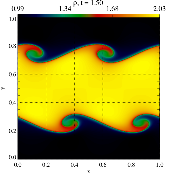
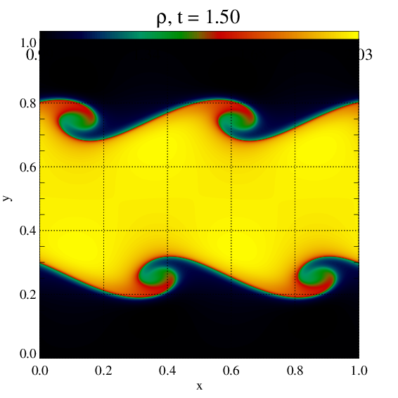
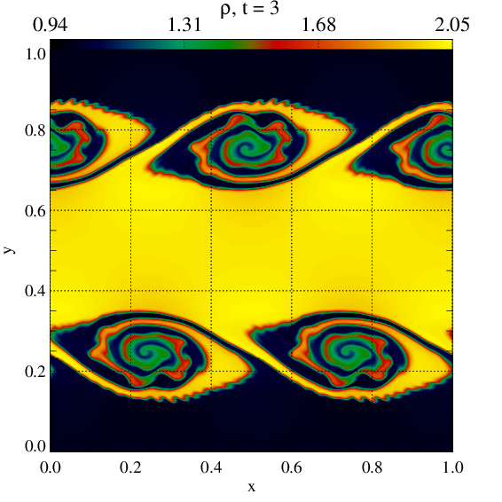
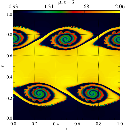
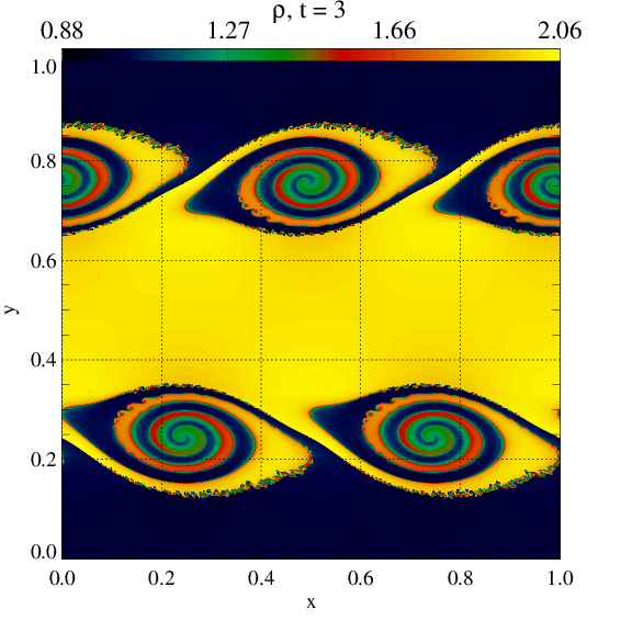
Figure 2: Density maps at $t=1.5$ (top) and $t=3$ (bottom) of the non-viscous runs with, from left to right, $n=256,1024,4096$.

The top panel of Fig. 1 shows the time evolution of the mode amplitude $M$ of several models without (solid lines) and with (dashed lines) explicit viscosity. The reference run (solid black line) and all simulations with a viscosity $\nu\leq 10^{-5}$ evolve in a very similar way with only small quantitative differences. After a transient decrease, $M$ starts to rise at $t\approx 0.4$. The increase proceeds at first exponentially with time. It slows down after $t\approx 1.3$ and reaches a maximum at $t\approx 2.1$. During this phase, the flow develops the characteristic KH vortices (see the density maps at $t=1.5$ in the top panels of Fig. 2) After the saturation of growth, $M$ gradually declines. The vortices continue to wind up and secondary instablities grow on the thin filaments around their centres (for $t=3$, see bottom panels of Fig. 2). Similarly to [3] and [4] (cf. their Fig. 10), we can distinguish between instabilities of the outer filaments and those of the inner core. The latter develop near the centres of the vortices, while the former appear near their edges. As found by [3] and [4], the outer filament instabilities are present at all resolutions, whereas the inner core instabilities grow slower at higher resolution to finally disappear for $n=4096$.

The growth of the KHI is noticeably smaller for very high physical viscosity of $\nu=10^{-4}$ and completely absent for $\nu=10^{-3}$. In these cases, the diffusion times for smearing out the shear layers is roughly $\tau_{\mathrm{diff}}\sim\frac{L^{2}}{\nu}=6.25\frac{10^{-4}}{\nu}$, i.e., of a similar order of magnitude as the growth time scale of the KHI. Diffusion decreases the gradient of $v^{x}$ across the shear layer, providing an additional decrease of the development of the KHI ($\nu=10^{-4}$) or even completely suppressing it ($\nu=10^{-3}$). Evidence for this explanation was found in auxiliary simulations in which the viscosity only operates on the difference of the velocity from its initial state. With diffusion of the shear layer thus eliminated, the additional suppression of the KHI is absent.

Since, except for the highest viscosities, all runs display a very similar evolution during the linear growth phase, we can use this stage without further complications in a convergence study. To this end, we examine the deviation from the reference, $D$, run until $t=1.5$. As shown in the bottom panel of Fig. 1, $D$, and hence ${E_{1.5}}$, approach $0$ as $n\to 4096$.

The left panel of Fig. 3, displaying $E_{1.5}$ as a function of viscosity for runs with different resolutions, displays two limiting behaviours. At high viscosity, $E_{1.5}$ follows a linear relation, $E_{1.5}\propto\nu$ that is common for all grids. The deviation of simulations at $\nu=10^{-3,4}$ from this trend owes itself to the smearing out of the shear layer due to rapid diffusion. If $\nu$ is decreased below a resolution-dependent threshold, $E_{1.5}$ levels off and approaches the value of the simulation in ideal HD, for which the diffusion is entirely due to numerical errors.

We can surmise that this numerical finding represents a physical result, i.e., that dissipation in the growth phase of the KHI operates in such a way that $E_{1.5}$ increases linearly with the viscosity. In our setup, the scaling is

$$E_{1.5}\approx 0.27\frac{\nu}{10^{-5}}.$$ (22)

The close similarity between a simulation in ideal HD and one oln a finer grid, but with physical viscosity, serves as an indication that the numerical errors indeed behave like a physical viscosity, which allows us to apply the scaling relation, Eq. (22), to determine the effective numerical viscosity of the code. The results, shown in Fig. 4, suggest for runs with MP5 reconstruction a power-law dependence of the numerical viscosity, $\nu_{\mathrm{num}}$, on the resolution:

$$\nu_{\mathrm{num}}=2.5\times 10^{-8}\left(\frac{n}{1024}\right)^{-2.25}.$$ (23)

The numerical errors of runs with second-order TVD piecewise-linear (PLM) reconstruction depend on resolution in a less straightforward way (orange line). For the finest grids ($n\geq 512$), we find a slightly shallower scaling relation $\nu_{\mathrm{num}}\propto n^{-1.75}$ at about one order of magnitude above the MP5 runs. The deviations from the scaling at the coarsest grids are stronger than for runs with MP5, even going so far as to change sign between $n=256$ and $n=512$.

We note that other elements of the numerical scheme such as the time integrators, CFL number, and Riemann solvers have a smaller influence on $E_{1.5}$ then the reconstruction method.

Applying the same analysis to the entire simulation time (for $E_{3}$, see the right panel of Fig. 3 and for the resulting numerical viscosity the right panel of Fig. 4), we find convergence as for $E_{1.5}$. Like before, $E_{3}$ depends linearly on the physical viscosity,

$$E_{3}\approx 0.96\frac{\nu}{10^{-5}}.$$ (24)

The inner vortex instabilities present at all but the finest grid complicate the interpretation of the results. They lead to a comparatively strong difference between the late stages of the runs with $n\leq 2048$ and the reference run, which is reflected in the upturn of the black curve in the right panel of Fig. 4. Simulations with the generally more viscous PLM schemes, on the other hand, suppress inner-core instabilities and, to a lesser degree, also outer-filament instabilities. Since the absence of inner-vortex instabilities renders the series of PLM runs close to the reference run, the total error, $E_{3}$, the difference between their numerical viscosity and that of the MP5 runs is relatively low.

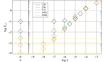
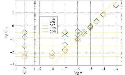
Figure 3: Left: Time-integrated deviation from the reference run, $E_{1.5}$, for simulation series with different resolutions (colours) as functions of viscosity (all with MP5 reconstruction). The horizontal yellow lines show the value of $E_{1.5}$ in the simulations in ideal HD. The inclined yellow line displays a linear relation $E_{1.5}\propto\nu$. Right: The same, but for $E_{3}$.

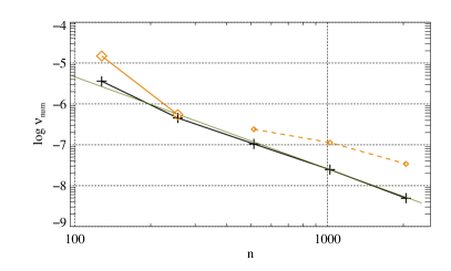
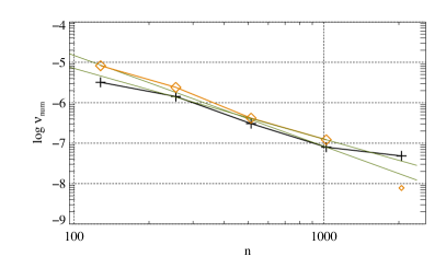
Figure 4: Left: The effective numerical viscosity of ideal-HD runs as a function of grid resolution. Black and orange symbols correspond to runs with MP5 and PLM reconstruction, respectively. For the latter group of runs, $E_{1.5}$ changes sign between $n=256$ and $n=512$. The two domains with different signs are distinguished by line styles. The green line represents the power law approximation Eq. (23). Right: same for $E_{3}$.

4 Summary and conclusions

We estimated the numerical viscosities of simulations of the non-magnetic KHI in two spatial dimensions based on several series of simulations varying the grid resolution by a factor of 32. In a first step, we determined the dependence of the amplitude of the mode excited by the initial perturbations on the physical viscosity. This result was then applied to assess the effective numerical viscosity of simulations in ideal HD. This procedure works very well in the early phase of the evolution, during which the KHI grows exponentially. We find a power-law scaling of the numerical viscosity on the grid resolution with an exponent slightly above and slightly below 2 for runs with high-order MP5 and second-order PLM reconstruction, respectively. After the termination of the growth, however, the dynamics is more complex, involving the appearance of secondary instabilities on the KH vortices. Their growth rates depend strongly on the resolution and differ between reconstruction methods, causing the same analysis to yield worse results than in the earlier phase. We note that The ansatz of Eq. (1) is only well motivated in the linear regime. Its applicability in the saturated phase requires additional study.

This relative failing of the method hints towards the necessity of applying the same rigorous analysis used for, e.g., the tearing-mode instability by [1]. We suspect that, instead of determining the global diffusive/dissipative error of a model, a breakdown of their dependence in terms of the characteristic velocity and length scales would serve to explain the nature of numerical viscosity. Such an analysis would be particularly helpful for the development or suppression of the secondary instabilities, which grow on much shorter length scales as the primary KHI. While this kind of study would thus be worthwhile for the non-linear saturated state, it is beyond the scope of this article. Further relevant extensions might focus on the effect of magnetic fields and three-dimensional systems.

Bibliography

Bibliography

- [1] Rembiasz T, Obergaulinger M, Cerdá-Durán P, Aloy M Á and Müller E 2017 ApJS 230 18
- [2] Suresh A and Huynh H 1997 J. Comput. Phys. 136 83–99
- [3] McNally C P, Lyra W and Passy J C 2012 ApJS 201 18
- [4] Lecoanet D, McCourt M, Quataert E, Burns K J, Vasil G M, Oishi J S, Brown B P, Stone J M and O’Leary R M 2016 MNRAS 455 4274–4288
- [5] Obergaulinger M 2008 Astrophysical magnetohydrodynamics and radiative transfer: numerical methods and applications Ph.D. thesis Technische Universität München
- [6] Evans C R and Hawley J F 1988 ApJ 332 659–677
- [7] Just O, Obergaulinger M and Janka H T 2015 MNRAS 453 3386–3413
- [8] Aloy M A, Ibáñez J M, Sanchis-Gual N, Obergaulinger M, Font J A, Serna S and Marquina A 2019 MNRAS 484 4980–5008